80

CHAPTER 4

INFLUENCE OF FLOW CONTROL AND COOLING ON

SUBMERSIBLE INDUCTION MOTOR

4.1 INTRODUCTION

Power consumption per hectare for any crop depends on the factors,

namely, horse-power-rating of the pump-set, water level of the well or the

tube-well, capacity of the pump, size of the delivery pipes, condition of the

water extraction machineries, distance between the place of the water-source

and the field to be irrigated, quality of the soil, terrain condition, and the

water-resource etc. These factors vary considerably across regions. Higher

horse-power pump-sets lift more water from the well than the lower horse-

power pump-sets. The water outlet of the pump-set is directly used for

irrigation, if the water availability is more, and this is called Flood Method

Irrigation (FMI). To increase the irrigation efficiency, now-a-days, the Drip

Method of Irrigation (DMI) is employed. The consumption of water by the

crops under DMI is significantly less compared to that of FMI. Since the

water is supplied through a pipe-network in DMI, mainly using groundwater,

the water supply can be controlled easily. The pattern of water usage under

DMI is expected to be different with those of FMI. It is a known fact that due

to rapid energisation of the pump-set sand the cultivation of water-intensive-

crops that is widespread, the consumption of electricity by the agricultural

sector has increased manifold since independence. Though the increased

consumption of electricity indicates better growth of the agriculture, many

researchers have reported that the electricity is not used efficiently in the

81

agriculture sector due to various reasons. One among the options available for

increasing the efficiency of electricity usage in agriculture is DMI.A few

preliminary level studies on DMI have shown that the micro-irrigation-

technology is not only useful for reducing the consumption of water, but also

useful in energy saving. DMI is efficient, if water-resource is good and

capable of supplying continuously. During the last forty years, India has been

witnessing a decline in gravity-flow-irrigation, and consequently, millions of

small private tube-wells have been put to use.

Further, enhanced use of groundwater has led to wells being bored

increasingly deeper, and farmers requiring higher-capacity pumps to lift

water. This extraction has not only increased the cost to the farmers and the

utilities, but progressively worsened the water availability in various regions.

Table 4.1 Availability of Ground-water in India

S. No.

Name of the State

Total No. of

Assessed Units

Safe Semi-critical Critical Over-exploited

No. of units % No. of

units % No. of units % No. of

units %

1 Andhra Pradesh 1231 760 62 175 14 77 6 219 182 Gujarat 209 97 46 69 33 12 6 31 153 Haryana 113 42 37 5 4 11 10 55 494 Karnataka 175 93 53 14 8 3 2 65 375 Kerala 151 101 67 30 20 15 10 5 36 Madhya Pradesh 312 264 84 19 6 5 2 24 87 Maharashtra 318 287 91 23 7 1 0 7 28 Punjab 137 25 18 4 3 5 4 103 759 Rajasthan 236 32 14 14 6 50 21 140 5910 Tamil Nadu 377 145 38 57 15 33 9 142 3811 Uttar Pradesh 803 665 83 88 11 13 2 37 412 Uttaranchal 17 12 70 3 18 0 0 2 12

Source: Dynamic ground water-resources of India

82

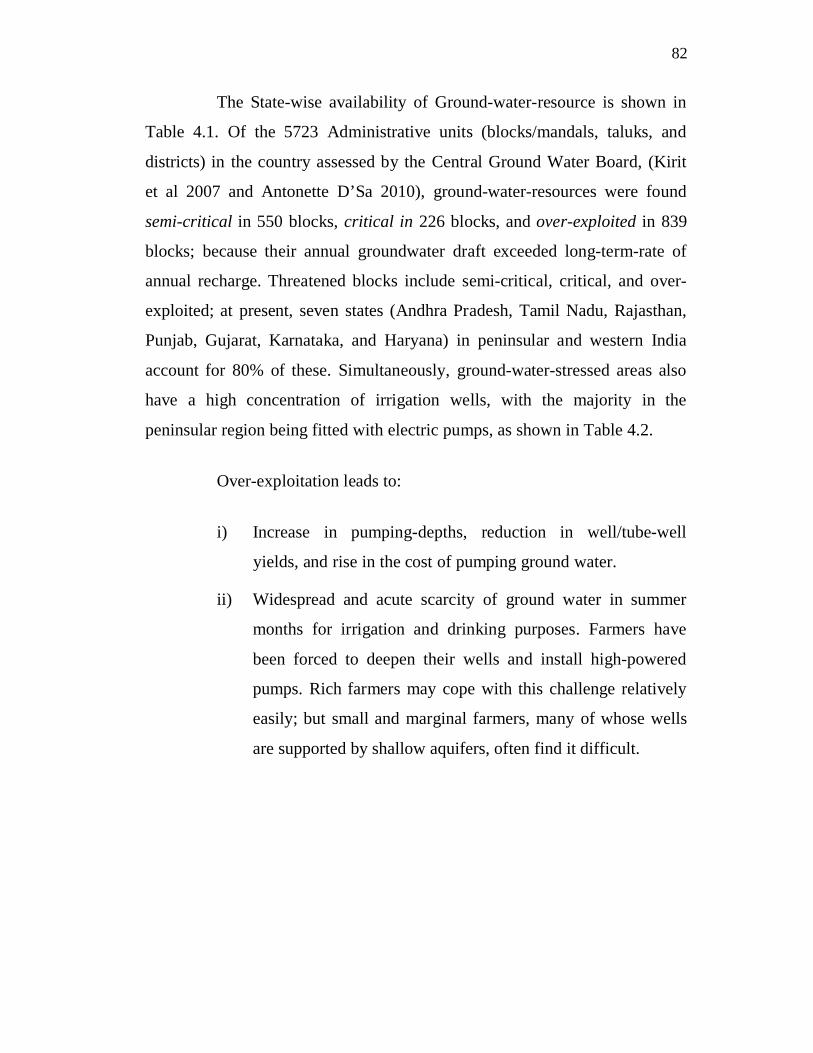
The State-wise availability of Ground-water-resource is shown in

Table 4.1. Of the 5723 Administrative units (blocks/mandals, taluks, and

districts) in the country assessed by the Central Ground Water Board, (Kirit

et al 2007 and Antonette D’Sa 2010), ground-water-resources were found

semi-critical in 550 blocks, critical in 226 blocks, and over-exploited in 839

blocks; because their annual groundwater draft exceeded long-term-rate of

annual recharge. Threatened blocks include semi-critical, critical, and over-

exploited; at present, seven states (Andhra Pradesh, Tamil Nadu, Rajasthan,

Punjab, Gujarat, Karnataka, and Haryana) in peninsular and western India

account for 80% of these. Simultaneously, ground-water-stressed areas also

have a high concentration of irrigation wells, with the majority in the

peninsular region being fitted with electric pumps, as shown in Table 4.2.

Over-exploitation leads to:

i) Increase in pumping-depths, reduction in well/tube-well

yields, and rise in the cost of pumping ground water.

ii) Widespread and acute scarcity of ground water in summer

months for irrigation and drinking purposes. Farmers have

been forced to deepen their wells and install high-powered

pumps. Rich farmers may cope with this challenge relatively

easily; but small and marginal farmers, many of whose wells

are supported by shallow aquifers, often find it difficult.

83

Table 4.2 Irrigation Wells in the Peninsular Region

Name of the State

Number of Irrigation-

Wells

Wells with Electrical

Pumps

Number of critical and over-exploited blocks

Andhra Pradesh 1929057 1691502 296

Gujarat 1082977 568117 43

Karnataka 860363 807377 68

Rajasthan 1341118 510020 190

Tamilnadu 1891761 1412697 175

Rest of India 18503268 9943486 1065

4.2 EFFECT OF DISCHARGE ON POWER CONSUMPTION

The efficiency of the agricultural submersible-pump-set is in the

range of 45% to 55% during its maximum discharge. This is possible only

with very few bore-wells which have very good water-resources. From

Table 4.1, it is clear that, in many places, the bore-wells are being operated

with poor water-resources and this leads to low water discharge mode of

pumps; this again is the cause for the poor efficiency and hence, the power

loss. By avoiding such low discharge mode of operation in water pumping,

energy could be conserved.

The water discharge of the pump from the bore-well at the time of

starting is more due to stagnant water. As the time passes, the water discharge

from the pump gets reduced due to the poor water-resource. In such

circumstances, the pumps are operated continuously with less discharge, and

the tank or the mud-reservoir is employed to store the water. After storage,

the water is used to irrigate the field. The performance report of 7.5-HP

submersible pump-set is shown in Table 4.3.

84

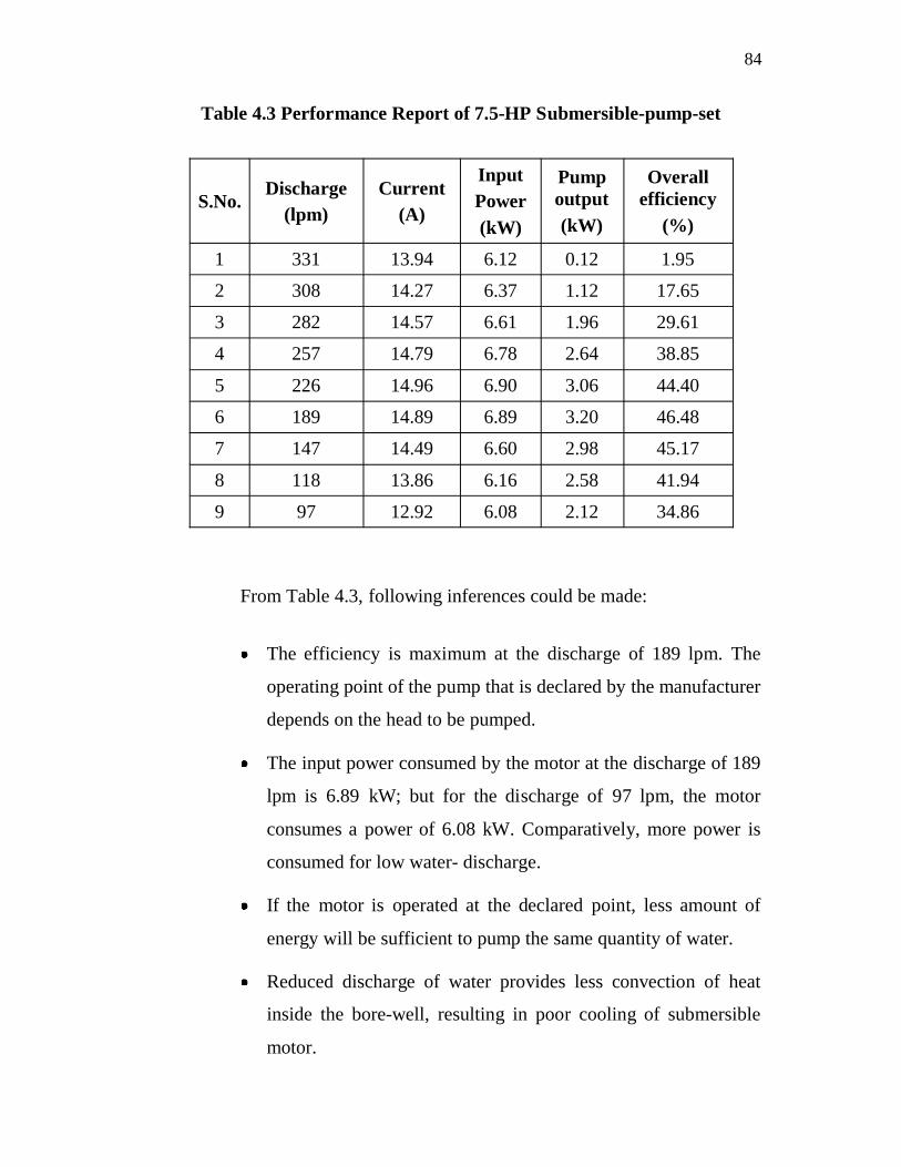
Table 4.3 Performance Report of 7.5-HP Submersible-pump-set

S.No.Discharge

(lpm) Current

(A)

Input Power (kW)

Pump output (kW)

Overallefficiency

(%)

1 331 13.94 6.12 0.12 1.95

2 308 14.27 6.37 1.12 17.65

3 282 14.57 6.61 1.96 29.61

4 257 14.79 6.78 2.64 38.85

5 226 14.96 6.90 3.06 44.40

6 189 14.89 6.89 3.20 46.48

7 147 14.49 6.60 2.98 45.17

8 118 13.86 6.16 2.58 41.94

9 97 12.92 6.08 2.12 34.86

From Table 4.3, following inferences could be made:

The efficiency is maximum at the discharge of 189 lpm. The

operating point of the pump that is declared by the manufacturer

depends on the head to be pumped.

The input power consumed by the motor at the discharge of 189

lpm is 6.89 kW; but for the discharge of 97 lpm, the motor

consumes a power of 6.08 kW. Comparatively, more power is

consumed for low water- discharge.

If the motor is operated at the declared point, less amount of

energy will be sufficient to pump the same quantity of water.

Reduced discharge of water provides less convection of heat

inside the bore-well, resulting in poor cooling of submersible

motor.

85

4.3 IMPLEMENTATION OF ELECTRONIC CONTROL IN

IRRIGATION

The flow-based / discharge-based automatic ON / OFF control of

submersible motor is used to conserve energy in critical and over-exploited

water- resource areas. Irrigation control has been incorporated in motor starter

with Flow sensor, Moisture sensors, and Solenoid valves so as to improve the

utilization of water and power consumption in the agriculture sector. The

block diagram of automated irrigation and water pumping system is shown in

Figure 4.1. The proximity type flow sensor is used to sense the discharge-

flow-rate; the water level sensors are used in the tank or mud-reservoir to

sense the water storage level. Discharge, water level, and moisture conditions

are monitored by the controller. The submersible pump is controlled by the

controller using power-driver circuit. The solenoid valves have been

employed to control the field irrigation system.

Figure 4.1 Block Diagram of Automated Pumping and Irrigation System

86

The basic operation of the controller is described in Figure 4.2 to Figure 4.5.

Figure 4.2 Flowchart for Controller Initialization and Function

Figure 4.3 Flowchart for Sensing of Parameters

START

Initialize the Microcontroller&Select the Clock frequency

Configure the Input andOutput Ports

Configure ADC to read Soil Moisture content

Configure the LCD Display

Read the Inputs(A)

Input processing,Decision making, and

Output updation (B)

Update the LCD Display

Read the Inputs(A)

Read the User Key Status

Read the Soil Moisture data from ADC

Read Water Level in Mud-reservoir

Read submersible pump discharge-rate

Return the Values

87

Figure 4.4 Flowchart for Controller operation

Low / Mid

Field irrigation(D)

Do Manual Functions(C)

Input processing, Decision making, and Output updation(B)

Mode

Field Moisture

ManualAuto

High Low

Water level in Mud-reservoir

Sub-Motor Status

Water level in Mud-reservoir

High

Low High / Mid

OFF

ON OFF

Switch OFF Sub-Motor

Switch ON Sub-Motor

Sub-MotorStatus

ON Pump-discharge> Set-value

Wait for Bore-well Refill (As per pre-set)

No

Yes

Switch OFF ‘S’

Return the Status

Switch OFF Sub-Motor

88

Figure 4.5 Flowchart for Sub-functions C and D

where ‘S’ –Main Solenoid valve

‘S1’ – Solenoid valve for Field -1 (F1)

‘S2’ – Solenoid valve for Field -2 (F2)

Yes

Switch ON‘S’, ‘S1’ Switch OFF‘S2’

Do Manual Functions(C)

Input

Is Sub-ON key pressed?

Valid Invalid

No

Irrigation Field selection

F1 F2

Return the Status

Switch OFF Sub-Motor, ‘S’, ‘S1’, and ‘S2’

Switch ON Sub-Motor

Switch ON‘S’, ‘S2’ Switch OFF‘S1’

No

Field irrigation (D)

Is F1.MC < F2.MC

Switch ON ‘S’

Read F1.MC and F2.MC, the respective Moisture Contents of Field-1 and

Field-2

Yes

Switch ON‘S1’ Switch OFF‘S2’

Switch ON‘S2’ Switch OFF‘S1’

Return the Status

89

The different subsystems of the electronic irrigation control system are:

Flow sensor

Moisture sensor

Solenoid valve

Control circuit

The Flow-meter PDLC4020, shown in Figure 4.6, manufactured by

Frehnig Instruments and Controls, Coimbatore, is used as a flow sensor. The

paddle wheel sensor is attached with the flow sensor, rotating on a long-life-

bearing and shaft. The sensor has three types of configuration, namely,

flanged-end- configuration, screwed-end-configuration, and OEM weldable

fittings. In all the three configurations, the sensor is of insertion type, enabling

ease of inspection and maintenance.

Figure 4.6 PDLC4020 Flow-meter

The specifications of the flow sensor are:

Accuracy: +/- 2.0%, Repeatability: +/- 1.0%,

Flow range: 0.3 m/sec to 7 m/sec, Pipe size: 19 mm to 300 mm.

90

Wheatstone bridge is used as the moisture sensing circuit. The

resistance of the soil is directly proportional to the soil moisture content. The

electrode is used to measure the moisture content and it is connected to the

Wheatstone bridge.

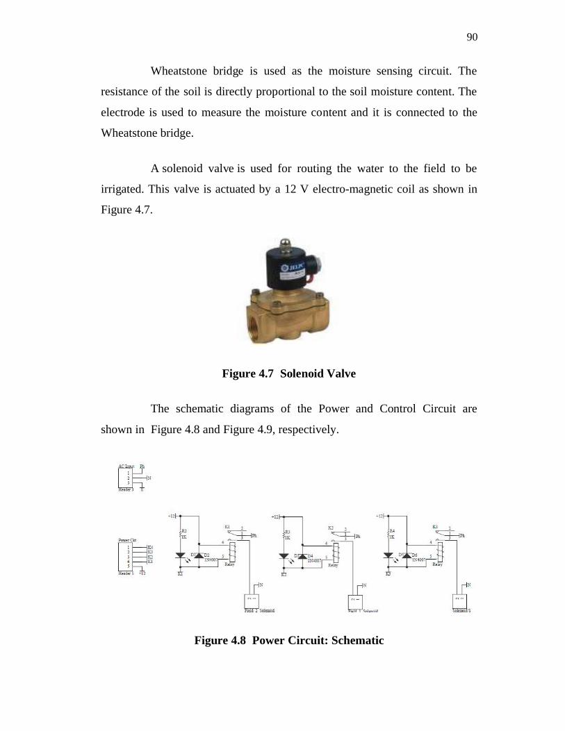
A solenoid valve is used for routing the water to the field to be

irrigated. This valve is actuated by a 12 V electro-magnetic coil as shown in

Figure 4.7.

Figure 4.7 Solenoid Valve

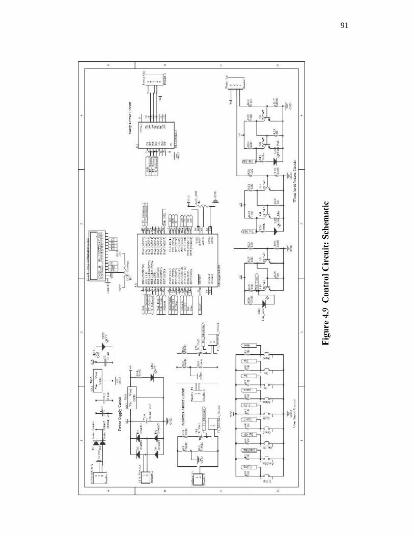
The schematic diagrams of the Power and Control Circuit are

shown in Figure 4.8 and Figure 4.9, respectively.

Figure 4.8 Power Circuit: Schematic

91

92

The PCB Layout Diagram for the Control Circuit is shown in Figure 4.10 and

Figure 4.11 shows the corresponding 3-D View.

Figure 4.10 Control circuit: PCB Layout

Figure 4.11 Control circuit: 3-D View

93

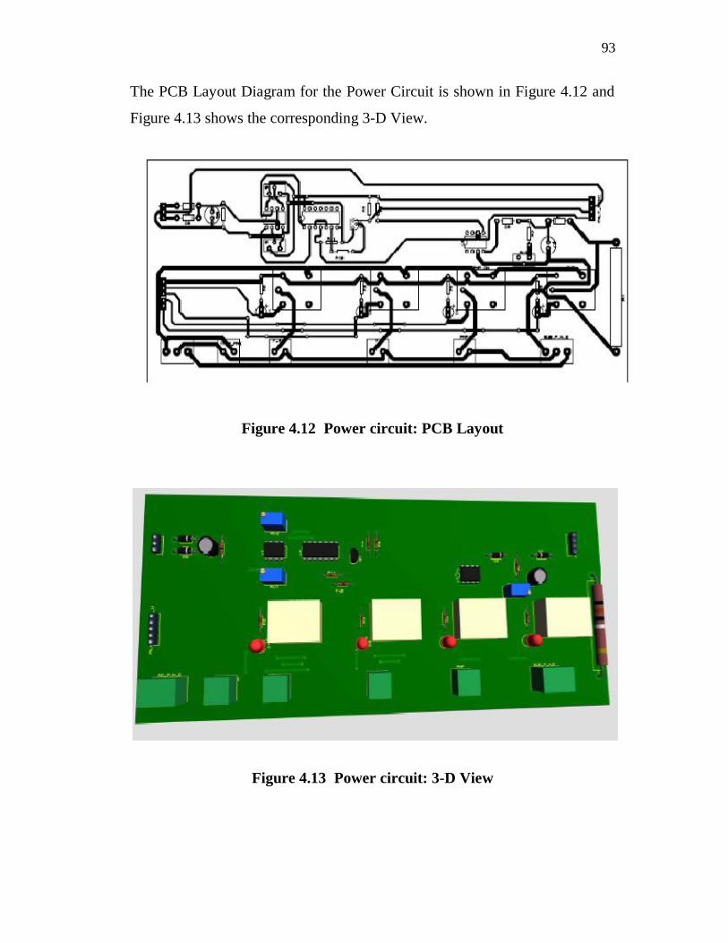
The PCB Layout Diagram for the Power Circuit is shown in Figure 4.12 and

Figure 4.13 shows the corresponding 3-D View.

Figure 4.12 Power circuit: PCB Layout

Figure 4.13 Power circuit: 3-D View

94

4.4 TEST RESULTS

The Electronic Flow Control mechanism was fixed with a 7.5-HP,

20-stage Submersible pump-set in an agriculture field at Siruvalur village,

Gopichetipalayam Taluk. The performance of the Submersible pump-set

without flow control mechanism is given in Table 4.4.

Table 4.4 Performance of Pump without Flow Control

Time of operation

Duration(h)

Status of the

Pump

Discharge (lps)

Quantity of water Pumped

(kL)

Energy Consumed

(kWh)

6.00 - 6.30 0.50 ON 4.50 8.10 3.326.30 -7.00 0.50 ON 4.20 7.56 3.297.00 -8.00 1.00 ON 2.45 6.82 6.718.00 -16.00 8.00 ON 1.80 51.84 48.40

16.00 -18.00 2.00 ON 2.00 14.40 12.32Total 12.00 88.72 74.04

It could be concluded from the parameters in Table 4.4, that the

discharge of the pump is not in the declared range to have a good efficiency,

because of the poor water resources, resulting in increased power

consumption. The performance of Submersible pump-set with flow control

mechanism is given in Table 4.5.

95

Table 4.5 Performance of Pump with Flow Control

Time of operation

Duration(h)

Status of the Pump

Discharge (lps)

Quantity of water

Pumped (kL )

Energy Consumed

(kWh)

6.00 - 6.30 0.50 ON 4.50 8.10 3.32

6.30 -7.00 0.50 ON 4.20 7.56 3.29

7.00 -7.30 0.50 ON 3.50 6.30 3.44

7.30 -8.00 0.50 OFF 0.00 0.00 0.00

8.00-9.30 1.50 ON 4.00 21.60 10.17

9.30-10.00 0.50 ON 3.50 6.30 3.44

10.00- 11.00 1.00 OFF 0.00 0.00 0.00

11.00-13.00 2.00 ON 3.50 25.20 13.58

13.00-14.00 1.00 OFF 0.00 0.00 0.00

14.00- 16.00 2.00 ON 3.50 25.20 13.58

16.00- 17.00 1.00 OFF 0.00 0.00 0.00

17.00-18.00 1.00 ON 3.50 12.60 6.87

Total 12.00 112.86 57.69

Following inferences could be made from Table 4.5:

The quantity of water pumped got increased by 21.3% in half

a day

Energy consumption of submersible pump set got reduced by

28% for a 12 hour duration, with 21.3% more water discharge

This would help reduce the total electricity bill to be paid by the

farmers. Farmers have to be educated on the conservation of water and

electrical energy. If this intelligent system is fitted along with the submersible

motor starter, will provide information on the water requirement to the

96

agriculture field and the energy requirement / consumed by the utility from

time to time; this will result in optimum utilization of electrical energy. The

decision making system should be supplied with the data on crop-pattern,

rain-fall-pattern and land-pattern for further improvement in energy

conservation. This system automatically shuts off the pump motor by sensing

the humidity and the moisture content of the land under irrigation.

4.5 COOLING OF SUBMERSIBLE MOTOR IN V6–TYPE

ASSEMBLY

The 3-phase squirrel cage Induction motor that is part of the

V6-type submersible pumps, has a slotted stator in which PVC-insulated

copper wire is inserted. The rotor consists of a series of skewed copper rods

welded together. Both the stator and the rotor are secured inside the water-

proof housing. The additional parts inside the housing are used to reduce the

run-out of the shaft.

Since the motor is not 100% efficient, a part of the power supplied

gets converted into heat (Joule Heating). This is detrimental to the life of the

motor. To remove the heat from the elements, the housing is filled with pure

water, so that no dirt particles block the clearance spaces between the rotor

and the stator. This heat, absorbed up by the water, gets transferred to the

ambient, and hence prevents the temperature rise inside the motor. Otherwise,

the heat may cause the insulation to melt and thereby short-circuiting the

wires. To enhance the heat transfer to the surroundings, the stator is covered

with a stainless steel casing. But, further efforts are necessary in order to

dissipate the heat effectively.

The key to increase the life of a submersible motor is to ensure

thermal conductivity at its best. Most submersible pumps rely on forced

convection in order to move heat away from the motor. The ambient/produced

97

fluid is typically drawn by the motor, in the course of pumping in order to

accomplish this task. The maximum motor diameter and the minimum inside

diameter of the well shall be in such a relationship that under any operating

condition, the water velocity past the motor neither exceeds 5.7 m/s nor goes

below 0.15 m/s.

Figure 4.14 Motor Jacket Installation with Cooling Sleeve

Figure 4.14 shows the motor jacket installation with cooling sleeve

used by most of the pump manufacturers worldwide. The shroud of the motor

is generally of the next nominal diameter of standard pipe larger than the

motor or the pump, depending on the shroud configuration used. The

tubular/pipe material can be plastic or thin-walled steel (corrosion resistant

materials preferred). The cap/top must accommodate power cable without

damage and provide a snug fit, so that only a very small amount of fluid can

be pulled through the top of the shroud. The fit should not be completely

water-tight as ventilation is often required to allow escape of the air or gas

that might accumulate. The shroud body should be stabilized so as to prevent

rotation and maintain the motor centered within the shroud. The length of the

98

shroud should extend to 1-2 times the diameter of the shroud beyond the

bottom of the motor. Shrouds are typically attached immediately above the

pump-intake or at the pump/column-correction. This type of sleeve is suitable

to standard conditions; but for wide operating voltage bandwidth and poor

water-resource areas, additional cooling mechanism is required so as to avoid

the failure of insulation. It has been reported by motor manufacturers of

Coimbatore that most of the insulation failure is at overhang portion of the

winding due to poor cooling.

4.5.1 Cooling by Forced Convection with Axial Fan

Heat dissipation can also be enhanced by increasing the flow-

velocity of the ambient fluid on the heat transfer surface. This process is

called forced convection. Increase in the flow velocity increases the

coefficient of convective heat transfer, which in turn increases the heat

transfer rate. To achieve this, axial fan (intended to give high flow rate) is

mounted on the shaft above the motor. For this, the length of the shaft needs

to be increased. The fan sucks water from beneath the motor, allowing it to

flow along the motor surface; finally, pushing it into the suction inlet of the

pump. The following parameters have been considered for the design of

7.5-HP submersible motor pump-set cooling:

Efficiency is of the order of 80 %

Heat dissipated is 0.2 x 7.5 x 0.746 = 1.11 kW

Speed of the motor is 2850 rpm

Motor is placed 350 feet below the ground level

Water temperature is 30ºC

The motor is assumed to be a constant temperature heat source

Specific Speed (Ns) for an axial fan is 7000 rpm

99

Head for the Axial fan is 2 m ( little greater than the pump

length )

Motor Outer Diameter (D1) is 140 mm

Bore Diameter (D2) is 165.1 mm

Thickness of casing (tc) is 7 mm, and Length of casing (Lc) is

426 mm

Thermal Conductivity of Cast Iron (Kci) is 80.13 W/m K

Properties of water at 30o C are:

Density ( d) is 995.7 kg / m3

Dynamic Viscosity ( d) is 7.975 x 10-4 N-sec/m2

Prandtl Number (Pr) is 5.43

Thermal Conductivity (kw) is 0.613 kW/m/K

The specific speed is given by Equation (4.1).

= . (4.1)

Substituting the values in Equation (4.1), the value of flow rate (Qf) is given

by

= 101.36

= 6.39

The area between the bore and the motor body (annulus) is given by

Equation (4.2).

100

= ( ) (4.2)

= 6.014 × 10

The velocity in the annulus is determined by Equation (4.3).

= (4.3)

= 1.06 m/s

The hydraulic diameter (Dh) is the difference between the diameter of the pipe

and the diameter of the motor body as given in Equation (4.4).

= (4.4)

= 25.1 mm

The Reynolds number (Re) is given by Equation (4.5).

= (4.5)

= 33361.75

Darcy’s friction factor (f) is given by Equation (4.6).

= (0.79 ln( ) 1.64) (4.6)

= 0.023

101

Nusselt number (Nu) is given by Equation (4.7).

=( )

..

(4.7)

= 211

The heat transfer coefficient (h) is calculated using Equation (4.8).

= (4.8)

= 5.153 kW (m2K)

The overall heat transfer coefficient (hoa) is determined by using

Equation (4.9).

= ××

(4.9)

= 3.553 kW (m2K)

The heat to be dissipated (H) and the surface area (As) are calculated using

Equation (4.10), and Equation (4.11), respectively.

= 0.2 × 7.5 × 0.746 (4.10)

= 1.119 kW

= 2 × × 0.140 × 0.426 (4.11)

= 0.37 m2

The Temperature Difference ( T) is calculated by Equation (4.12)

102

= (4.12)

= 1.68 K

The following assumptions have been made in the design of the

axial fan so as to increase the flow velocity:

Usually, Dhub/Dtip is in the range of 0.3 to 0.6, and 0.55 is

considered for this case.

Inlet Pre-whirl = 0

Dtip = 70 mm

Number of blades (Zb) = 3

The diameter of the hub (Dhub) is calculated using the tip diameter (Dtip) and

the ratio as given in Equation (4.13).

D = 0.55 × D (4.13)

= 38.5 mm

The flow area (Af) between the hub and the tip of the fan is determined by

Equation (4.14).

= (4.14)

= 0.002684

The meridional component (Cm) of the velocity in terms of

discharge and area is calculated using Equation (4.15).

103

= (4.15)

= 2.38 m/sec

The blade tip velocities U1 and U2 at the hub (h) and the tip (t) at both the

inlet (1) and the exit (2) are found by using Equation (4.16) and Equation

(4.17), respectively.

= = × × × .×

(4.16)

= 10.44 m/sec

= = × × × .×

(4.17)

= 5.745 m/sec

Both the Exit Whirl-hub (Cu2h) and the Exit Whirl-tip (Cu2t) are

assumed as 19.6 m/sec, based on the axial fan head of 2 m.

The hub blade angle at the inlet is calculated using

Equation (4.18).

= (4.18)

= 22.5º

The tip blade angle ( 1t) at the inlet is calculated using

Equation (4.19).

= (4.19)

= 12.84º

104

The hub blade angle ( 2h) at the exit is calculated using Equation (4.20).

= (4.20)

= 45.46º

The tip blade angle at the exit is calculated using Equation (4.21).

= (4.21)

= 15.53º

From graphs (Stephanhoff), the vane spacing ratios at the hub and

the tip are found to be 0.975 and 1.2675, respectively.

The vane spacing at the hub (thub) and the tip (ttip) are determined by

using Equation (4.22) and Equation (4.23), respectively.

= (4.22)

40.31 mm

= (4.23)

73.33 mm

The vane chord length of tip (ltip) and the van chord length of hub

(lhub) are calculated using the vane spacing ratio and the vane spacing at the

hub (thub), and the tip (ttip) as:

ltip 71.46 mm

lhub 39.30 mm

105

The 3-D model of the axial fan, the new intermediate piece, and the

axial fan assembly is shown in Figure 4.15. Assembly view of axial fan with

the Motor is shown in Figure 4.16.

Figure 4.15 Axial Fan Assembly: 3-D Model

Figure 4.16 Axial Fan with the Motor: Assembly View

The aluminium die-casted axial fan is shown in Figure 4.17.

106

Figure 4.17 Axial Fan: Hand-casted Aluminum Model

Figure 4.18 Axial Fan, Motor, and Pump: Assembly View

The axial fan was fitted with the existing 7.5-HP submersible

pump-set by using an additional intermediate piece as shown in Figure 4.18.

The performance test was carried out in industry test-setup-sump with and

107

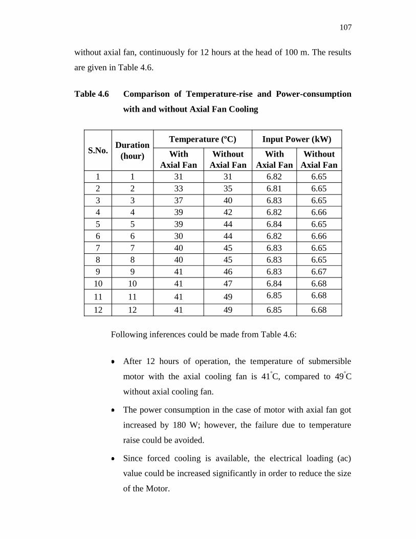
without axial fan, continuously for 12 hours at the head of 100 m. The results

are given in Table 4.6.

Table 4.6 Comparison of Temperature-rise and Power-consumption

with and without Axial Fan Cooling

S.No. Duration(hour)

Temperature (ºC) Input Power (kW)

With Axial Fan

Without Axial Fan

With Axial Fan

Without Axial Fan

1 1 31 31 6.82 6.652 2 33 35 6.81 6.653 3 37 40 6.83 6.654 4 39 42 6.82 6.665 5 39 44 6.84 6.656 6 30 44 6.82 6.667 7 40 45 6.83 6.658 8 40 45 6.83 6.659 9 41 46 6.83 6.6710 10 41 47 6.84 6.6811 11 41 49 6.85 6.68

12 12 41 49 6.85 6.68

Following inferences could be made from Table 4.6:

After 12 hours of operation, the temperature of submersible

motor with the axial cooling fan is 41ºC, compared to 49ºC

without axial cooling fan.

The power consumption in the case of motor with axial fan got

increased by 180 W; however, the failure due to temperature

raise could be avoided.

Since forced cooling is available, the electrical loading (ac)

value could be increased significantly in order to reduce the size

of the Motor.