42

Chapter 4

Methodology

This chapter is divided into six main sections, with each section discussing a particular

step taken in the methodology. The first five sections are dedicated to developing the data

needed to perform four BOD/DO modeling runs in the Upper HSC, while the final section

describes the procedure used to establish the GIS/WASP5 model connection. The first section

introduces the study area by describing the Upper Houston Ship Channel and its contributing

watershed. The second section provides a brief overview of water quality segmentation,

previous segmentations of the HSC, and the segments used for the water quality modeling

performed in this study. In addition, this section introduces the terminology of main segment

and boundary segment in relation to their use in this research.

Section 4.3 gives a procedure for the calculation of the non-point source loadings

entering the Upper HSC. This procedure uses land use-based estimated mean concentrations,

with spatially distributed runoff volumes to result in a areal loading of BOD to the Channel

from the watershed. This section also presents a method of estimating baseflow, given a daily

flow record and spatially distributing that runoff, using existing data and land use

characteristics. It is important to note that the loading calculation performed in this section

assumes that the non-point source load is only transported by the runoff volume. The following

section (Section 4.4) discusses the point source loadings to the modeled reach. Only those

dischargers located along the Upper HSC shoreline were considered in the point source loading

determination. In contrast to the non-point source loads, the point source loads were assumed

to be transported by the channel baseflow, which is discussed further in Section 4.5.

Section 4.5 presents the WASP5 model development, including determination of model

constants, estimation of water quality segment parameters, and execution of the model

calibration and model runs. Within the section, the channel flow, which is needed for the

43

WASP5 model, is discussed. This flow is spatially distributed in the same way as the runoff

was in Section 4.3. The final flow values for each segment, along with the corresponding runoff

values from Section 4.3, are used to determine the baseflow in each water quality segment.

This baseflow is necessary when looking at dry weather conditions, where just point source

loads are entering the system (i.e., no runoff or non-point source loadings). The four modeling

cases are also presented in this section: an average year case, a dry weather condition, and two

cases to test model sensitivity.

Finally, Section 4.6 discusses the WASP5/GIS model connection through the software

ArcView, while using Avenue and FORTRAN programming. The discussion presents the

menus created in ArcView to execute the Avenue scripts which read and write the model input

information from tables and coverages. This section also gives a step-by-step procedure, along

with an outline of the necessary tables and coverages, which is used to run the model

connection. This section also contains an overview of the WASP5 input blocks as they relate

to the interface, including assumptions and defaults set in the creation of the input file.

4.1 STUDY AREA

The model developed incorporated the Upper Houston Ship Channel and all land

draining into this section of the channel (Figure 4-1). Figure 4-1 also shows the major highway

systems in the Houston area for reference. The western boundary for the Upper HSC, the

Turning Basin, receives the majority of its input from Buffalo Bayou, whose watershed is

primarily covered by the greater metropolitan area of Houston. This water reach then travels

east, receiving water and loadings from the Brays, Sims, Berry, Green, Hall, Carpenter, and

Vince Bayous, and draining about 2600 km2 of land. The San Jacinto Monument creates the

eastern boundary of the 25 km section studied and is located just west of the confluence of the

San Jacinto River. For digital representation, the channel was depicted in GIS two ways: 1)

USGS Digital Line Graph (DLG); and 2) a segmented line drawn down the centerline of the

channel.

45

The DLG (Figure 4-1) depicts the Channel as a double-lined water reach; however, for

digital representation in GIS and modeling purposes, the channel is depicted as a single flow

line. Since the channel width averages only about 1000 meters at its widest point in that area, it

could be modeled in just two dimensions (length and depth). Because of this detail, a single

line could accurately be used to represent the channel in GIS. Therefore, a centerline was

manually-drawn onto the DLG and the shoreline of the Upper HSC deleted in the Arc/Info

subprogram, ArcEdit. Figure 4-2 shows the final result of this process. Section 4.2 further

discusses the centerline representation of the Channel in GIS.

4.2 CHANNEL SEGMENTATION

In order to model the channel in WASP5, it is necessary to divide the reach into water

quality segments. A segment is assumed to have uniform modeling parameters, such as depth,

cross sectional area, dispersion coefficients, etc. Each segment is considered to be a

completely mixed reactor. After the point and non-point loadings into each segment are

determined; these loads, along with the necessary physical and chemical parameters, are read

into WASP5 to produce a dissolved oxygen profile.

4.2.1 Previous Segmentation in the Houston Ship Channel

The Texas Water Commission (TWC -- now Texas Natural Resource Conservation

Commission -- TNRCC) divided the entire Galveston Bay System into 40 segments (Ward and

Armstrong, 1992). However, since the determination of these segments was controlled by

regulatory reasons, homogeneous hydrography within a TWC segment could not be assumed.

In addition, the reach considered for this study made up only two of the TWC segments (Figure

4-3). This resolution was not fine enough for an accurate modeling effort. Ward and

Armstrong (1992) further divided the Bay and Channel into smaller, hydrographic segments

(Figure 4-4). But, a full modeling effort, concerning DO had not been performed with this finer

segmentation. In another earlier study (Espey et al., 1971), the entire channel was divided into

28 segments (Figure 4-5), from the Turning Basin to Morgan’s Point (located at the mouth of the

Channel flowing into the main bay). The 1971 effort, performed by Tracor, Inc., modeled the

entire HSC for DO and BOD.

50

4.2.2 Segmentation Chosen

For this study, the Upper HSC reach was divided into eight of the hydrographic

segments developed in the Tracor Inc. modeling effort of the HSC (Espey, et al., 1971). By

using this segmentation, the results of the modeling from this present study could be compared

to the results of the 1971 study. Since this research considered just the Upper Houston Ship

Channel, only the first eight segments of the 1971 report were used as the main segments for the

modeling effort. Figure 4-6 shows the final segmentation used, while Table 4-1 gives some

general characteristics of each main segment. In addition, some of the information provided in

the 1971 report, concerning the incoming tributaries was used to develop the model boundary

conditions (see Sections 4.2.3 and 4.5).

Table 4-1 General Characteristics of the Main Segments used for the

Modeling Effort

Segment Length Cross-sectional Area Depth % Total

Number (km) (m2) (m) Length

1 3.1 1625.8 9.1 12.82 3.4 1625.8 9.1 14.13 1.9 1625.8 9.1 8.14 2.7 1625.8 6.1 11.45 3.7 1625.8 9.1 15.46 3.5 1625.8 6.1 14.87 2.4 2471.3 7.9 10.18 3.2 2471.3 7.9 13.4

Total 24.0Source: Espey,, et al., 1971

4.2.3 Segment Terminology in this Research

In this report, a main segment is a term used in reference to the eight water quality

segments described in the previous section and used to represent the 25 km of the Upper HSC

modeled in this study. In addition, nine boundary segments are defined in this research. Model

boundaries are those segments which import, export, or exchange water with the locations

outside the main network. A boundary segment represents either a tributary inflow, a

downstream outflow, a sediment layer, or an open water end of the model network across which

dispersive mixing can occur. Within GIS, arcs were defined to represent the Buffalo,

52

Brays, Sims/Berry, Hunting, Vince, Green/Hall, and Carpenter Bayous (see Figures 4-1 and 4-7)

to account for the tributaries entering the Upper HSC. The eighth boundary segment is the most

downstream segment, which includes an input from the San Jacinto River (segment #17). The

length of these arcs is arbitrary, but the lengths of the segments in the model are set at 3.2 km

for all but the Buffalo Bayou, which is set at 8 km. These actual lengths, which are defined in a

GIS table related to the arc coverage, are meant to depict infinite boundary conditions. Finally,

the ninth boundary segment (segment #9), represents the underlying sediment layer. Further

discussion on the main and boundary segments, their parameters, and their use in the model is

provided in Section 4.5.

4.2.4 Segmentation in GIS

Since the objective of this research was to connect WASP5 to GIS, the channel

segmentation needed to be digitally represented in Arc/Info and ArcView. As mentioned

earlier, the most efficient way to depict the channel was as a single line in GIS. As a result, the

channel was viewed in GIS as a stream, into which numerous other streams (i.e., bayous)

drained (Figure 4-6).

However, it was necessary to get GIS to recognize the channel as eight different

segments, instead of one long stream. The desired result was eight arcs, each carrying their

respective segment number as an attribute. To accomplish this task, a process called

“flowlength” in Arc/Info’s subprogram, Grid, was executed on the flow direction grid of the

DEM (see Section 4.3 for further explanation of the flow direction grid). The flowlength

command produced a grid in which each cell value corresponded to the distance, in meters,

from that respective cell to the ultimate outlet of the grid. The flowlength values for just the

single line representation of the Upper HSC were isolated with a Grid Boolean query (see

Procedure 4-1). The result of this effort was a “single-lined” grid of the Upper Houston Ship

Channel, with each 100m x 100m cell containing its respective flowlength value.

54

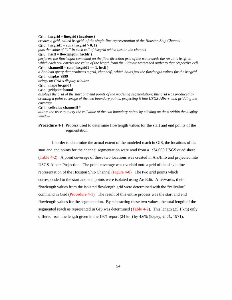
Grid: hscgrid = linegrid ( hscalone )creates a grid, called hscgrid, of the single-line representation of the Houston Ship ChannelGrid: hscgrid1 = con ( hscgrid > 0, 1)puts the value of “1” in each cell of hscgrid which lies on the channelGrid: hscfl = flowlength ( hscfdr )performs the flowlength command on the flow direction grid of the watershed; the result is hscfl, inwhich each cell carries the value of the length from the ultimate watershed outlet to that respective cellGrid: channelfl = con ( hscgrid1 == 1, hscfl )a Boolean query that produces a grid, channelfl, which holds just the flowlength values for the hscgridGrid: display 9999brings up Grid’s display windowGrid: mape hscgrid1Grid: gridpaint bounddisplays the grid of the start and end points of the modeling segmentation; this grid was produced bycreating a point coverage of the two boundary points, projecting it into USGS-Albers, and gridding thecoverageGrid: cellvalue channelfl *allows the user to query the cellvalue of the two boundary points by clicking on them within the displaywindow

Procedure 4-1 Process used to determine flowlength values for the start and end points of thesegmentation.

In order to determine the actual extent of the modeled reach in GIS, the locations of the

start and end points for the channel segmentation were read from a 1:24,000 USGS quad sheet

(Table 4-2). A point coverage of these two locations was created in Arc/Info and projected into

USGS-Albers Projection. The point coverage was overlaid onto a grid of the single line

representation of the Houston Ship Channel (Figure 4-8). The two grid points which

corresponded to the start and end points were isolated using ArcEdit. Afterwards, their

flowlength values from the isolated flowlength grid were determined with the “cellvalue”

command in Grid (Procedure 4-1). The result of this entire process was the start and end

flowlength values for the segmentation. By subtracting these two values, the total length of the

segmented reach as represented in GIS was determined (Table 4-2). This length (25.1 km) only

differed from the length given in the 1971 report (24 km) by 4.6% (Espey, et al., 1971).

56

Table 4-2 Start and End Points for Model Segmentation. Table also shows the flowlength values for each point and the resulting reach length in GISPoint Location Flowlength Value

(From 1:24,000 USGS Quad Sheet) (m)

Turning Basin 29° 44' 58.4" N 95° 17' 25.4" W 38654.648San Jacinto Monument29° 45' 24.5" N 95° 5' 20.0" W 13502.429

Difference: 25152.219Length of reach in GIS 25.1 km% Difference from Espey, et al. (1971): 4.6

Since the scale of the DLG may not have been on the exact same scale as the map used

to determine the 1971 segmentation, proportional segmentation was used. To accomplish this

task, the percent of the total reach length for each segment was calculated from the lengths

given in the 1971 report. Those percentages, as shown in Table 4-1, were then applied to the

total stream length of the arc within GIS, as determined from the procedure above. A detailed

description of this process is outlined in Procedure 4-2. The final result, as illustrated in Figure

4-6, was an eight-arc coverage of the segmentation, with each arc carrying an attribute

corresponding to its segment number.

Grid: seg_1 = con ( channelfl le 38654.648, 0) + con ( channelfl gt 35447.318, 1 )puts a value of “1”(1 + 0) in each cell that has a flowlength value (see Procedure 4-1) less than orequal to 36854.648 (the upper bound for segment one) and greater than 35447.318 (the lower bound);the total length of this segment is 12.8 % of the total segment length (see Table 4-1)Grid: seg_2 = con ( channelfl le 35447.318, 1) + con ( channelfl gt 31902.374, 1 )Grid: seg_3 = con ( channelfl le 31902.374, 1) + con ( channelfl gt 29876.692, 2 )Grid: seg_4 = con ( channelfl le 29876.692, 2) + con ( channelfl gt 27006.975, 2 )Grid: seg_5 = con ( channelfl le 27006.975, 2) + con ( channelfl gt 23124.418, 3 )Grid: seg_6 = con ( channelfl le 23124.418, 3) + con ( channelfl gt 19410.668, 3 )Grid: seg_7 = con ( channelfl le 19410.668, 3) + con ( channelfl gt 16878.562, 4 )Grid: seg_8 = con ( channelfl le 16878.562, 4) + con ( channelfl gt 13502.425, 4 )the above statements perform the same function as the first, only for each respective segment, theflowlength values change to encompass the necessary segment length and locationGrid: hsc_seg = merge ( seg_1, seg_2, seg_3, seg_4, seg_5, seg_6, seg_7, seg_8 )merges each individual grid, corresponding to each segment, into one gridGrid: segarc = gridline ( hsc_seg, #, #, #, #, grid-code )creates an arc coverage of the grid and stores the segment number in the aat under “grid-code”

Procedure 4-2 Commands used to segment the single line representation of the HSC into eightarcs.

57

Once the segmentation was recognized in GIS, the parameters of each segment were

attached to the attribute table of the eight-arc segmentation coverage. It was then possible for

GIS to read the necessary input parameters for the model run. This concept is further discussed

in Section 4.6.

4.3 NON-POINT SOURCE LOADS

Introduction

A non-point source (NPS) load is defined as any input into the HSC waters that is a

result of runoff, which flowed over the land and picked up constituents from the land surface.

Although the flow may have been channelized into a tributary by the time it reached the

Houston Ship Channel, if the constituents originated from the land surface, as opposed to an

outfall pipe, the load was considered to be a non-point source load. Determining the actual

loading of constituents caused by overland flow has been a subject of numerous reports

(Newell, et al., 1992; Saunders, 1996). The method used in this report is similar to procedures

described in Saunders (1996) and Newell, et al. (1992). The process utilized GIS to assist in

the non-point source loading calculations. The basic concept of the method incorporated the

following general equation:

Concentration (mass/volume) * Volume of Water (volume) = Load (mass) (4-1)

The method developed, discussed in more detail below, was a grid-based model that calculated

the non-point source load for each 100m x 100m cell of the watershed. The process used

values called Estimated Mean Concentrations (EMCs), which, when associated with land use

areas, provided the contribution of a given constituent to the runoff flowing over that area.

Actual runoff and precipitation measurements were compiled and correlated to help spatially

distribute the runoff over the entire 2600 km2 area. This distributed runoff, combined with the

land use based EMCs, established the NPS loadings into the Upper HSC.

58

The processed specifically incorporated the following steps:

• Delineate watershed area (total and area draining into each segment)

• Spatially distribute the runoff

• Determine land use and concentration (EMC) from each cell

• Use Equation (4-1) to determine loading from each cell

• Determine the NPS load into each water quality segment

These steps are discussed in more detail in the following paragraphs.

Watershed Delineation

The grid-based watershed delineation has been used in other projects to produce a

digital representation of all land draining into a body of water (Saunders, 1996). The concept in

the watershed delineation is the use of the 3″ DEM (see Section 3.2.3) to determine the

direction of flow over the surface terrain. The basis of this concept is the application of the

“eight direction pour point model” (Maidment, 1993). As shown in Figure 4-9, the eight

direction pour point model employs the theory that, if a drop of water falls onto a given cell, it

can flow in eight different directions. The direction chosen is that of the steepest slope. Once

the direction of the water flow is determined (termed the flow direction grid), Arc/Info’s

subprogram, Grid, accumulates the flow down to a given outlet (or the ultimate outlet of the

grid) by counting the number of cells upstream that flow into that particular cell. A stream

network is then delineated from a certain threshold value. In other words, a cell with a certain

minimum number of cells draining into it was considered part of the stream network. Procedure

4-3 shows a detailed description of this entire process in Grid. It is important to note that the

DEM used is one that has been projected into USGS-Albers and a 100m x 100m cell size

resolution. In addition, the point which represents the San Jacinto Monument was considered

the ultimate outlet of the study area; therefore, a grid containing one cell, corresponding to this

ultimate outlet point, was created through ArcEdit.

60

Grid: fill hscdem hscfil SINKfills any “pits” or large differences in elevations between neighboring cells that may cause delineationerrors. The "SINK" at the end of the statement tells Grid to look for cells which are lower than itssurrounding cells.Grid: hscfdr = flowdirection ( hscdem )creates a flowdirection grid of the dem; each cell carries a value which indicates the direction of flowfrom that cellGrid: hscfac = flowaccumulation ( hscfdr )creates a flowaccumulation grid of the flowdirection grid; each cell carries a value which correspondsto the number of cells that drain into itGrid: str_500 = con ( hscfac > 500, 1 )creates a grid of a stream network on the 500 level threshold; all cells that contain a flow-accumulation value of 500 or higher is considered part of the stream network and given a value of 1Grid: totalshed = watershed ( hscfdr, outlet )delineates the watershed from a given outlet point, in this case a grid containing one cell which islocated nearest to the San Jacinto Monument. The outlet grid was developed by creating a pointcoverage of the location of the San Jacinto Monument (Table 4-2) and then creating a grid which hasjust one cell, corresponding to the point location through ArcEdit.Grid: covstr_500 = streamline ( str_500 )Grid: covtotsd = gridpoly ( totalshd )converts the stream network grid and the watershed grid into line and polygon coverages, respectively

Procedure 4-3 Procedure used to delineate a watershed from a DEM for a given outlet.

The procedure above was determined using pure elevation data from the DEM.

However, the final product of this attempt produced a poor digital representation of the stream

network and watershed boundary (Figure 4-10). This erroneous result was mostly due to the

relatively flat terrain in the area. Therefore, it was necessary to “burn in” the streams, using a

cleaned 1:100,000 DLG. In this process, which is also employed in Saunders (1996), the

original DLG was edited in ArcEdit to eliminate any circular arcs (i.e., lakes, reservoirs, etc.)

and connect any dangling streams that are meant to be continuous. In addition, during the edit

process, instream lakes and double-lined rivers or channels were replaced with representative

streamlines. The streams were then gridded at the same resolution as the DEM (100m x 100m)

and the elevations in the DEM, except for the cells which corresponded to the DLG stream cells

were raised five meters. A new watershed could then be delineated, producing a more accurate

digital representation of the ridgeline (see Procedure 4-4). As done previously, the ultimate

outlet for this watershed was chosen to be a cell which was located nearest to the San Jacinto

Monument (i.e. the last cell found in

62

water quality segment eight). Figure 4-11 depicts the final watershed and stream network

resulting from this procedure.

Grid: dlggrid = linegrid ( dlgedit, #, #, #, 100, 0 )grids the edited DLG into 100m x 100m cells and places the value of zero in those cells notcorresponding to the streamsGrid: hscburn = con ( dlggrid > 0, 0, hscdem + 5 )increases the elevation values of the DEM grid by five meters and places the value of zero in any cellwhich corresponds to the stream networkGrid: fill hscburn hscfil SINKfills any “pits” or large differences in elevations between neighboring cells that may cause delineationerrorsGrid: hscfdr = flowdirection ( hscdem )creates a flowdirection grid of the dem; each cell carries a value which indicates the direction of flowfrom that cellGrid: hscfac = flowaccumulation ( hscfdr )creates a flowaccumulation grid of the flowdirection grid; each cell carries a value which correspondsto the number of cells that drain into itGrid: str_500 = con ( hscfac > 500, 1 )creates a grid of a stream network on the 500 level threshold; all cells that contain a flowaccumulationvalue of 500 or higher is considered part of the stream network and given a value of 1Grid: totalshed = watershed ( hscfdr, outlet )delineates the watershed from a given outlet point, in this case a grid containing one cell which islocated nearest to the San Jacinto MonumentGrid: covstr_500 = gridline ( str_500 )Grid: covtotsd = gridpoly ( totalshd )converts the stream network grid and the watershed grid into line and polygon coverages, respectively

Procedure 4-4 Procedure for “burning in” the DLG streams and delineating the correspondingwatershed.

The above procedures produced the total watershed (approximately 2600 km2).

However, the area draining into the segments described in Section 4.2 was of more importance

when determining the NPS loading into each of the eight reaches. As a result, an outlet was

defined at the downstream point of the segment, for each reach by locating the maximum

flowaccumulation value in each zone (i.e. water quality segment) of the segmentation grid (see

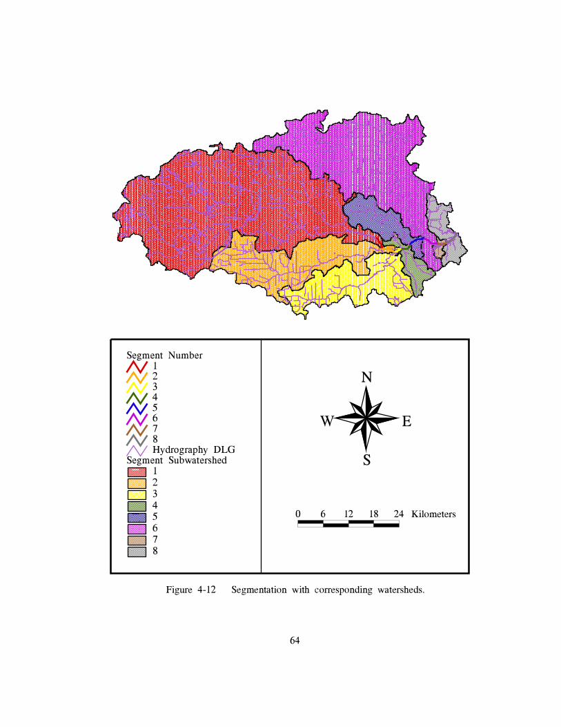
Procedure 4-5). The result was a grid of eight outlets, from which eight subwatersheds were

delineated. Figure 4-12 illustrates the final coverage of the areas draining into each segment,

while Table 4-3 gives the delineated areas for each subwatershed. Procedure 4-5 describe the

commands used in Grid to produce this result.

65

Table 4-3 Delineated Areas of Segment Subwatersheds

SegmentNumber

Area

(km2)

1 1143.982 330.593 241.434 58.215 111.736 635.767 10.048 74.69

Total 2606.43

Grid: acc_seg = zonalmax ( hsc_seg, hscfac )locates the maximum flowaccumulation value in each zone; in this case hsc_seg is a grid consisting ofeight zones -- one for each segmentGrid: out_seg = con ( acc_seg == hscfac, hsc_seg )places the values of the segment number in the cell which corresponds to the maximumflowaccumulation value; the result of this is the outlet gridGrid: seg_shd = watershed ( hscfdr, out_seg )delineates the watersheds for the eight given outlets

Procedure 4-5 Commands used to develop segment subwatersheds.

Spatial Distribution of Runoff

After the watershed was delineated, it was necessary to obtain an average runoff

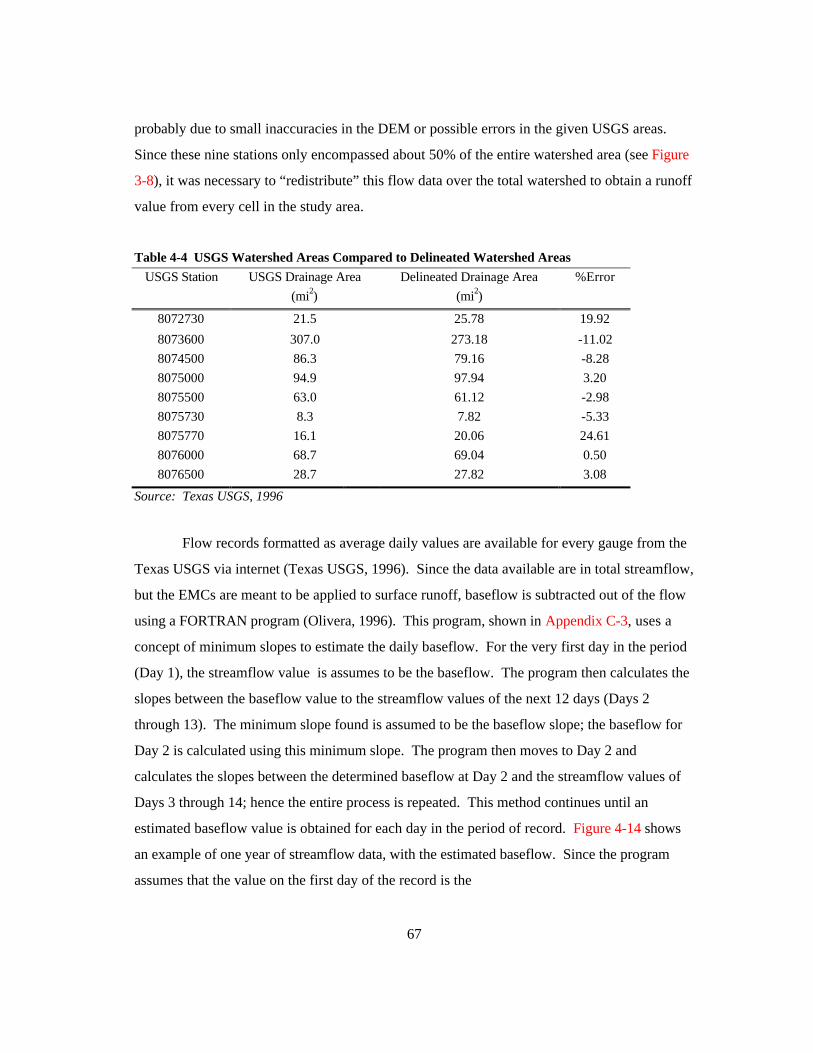
volume generated from each cell. As mentioned in Section 3.2.6, 37 USGS streamflow gauges

were located in the study area (Figure 4-13). Of these 37 gauges, nine were chosen for their

long period of records to determine a spatial distribution of runoff for the entire watershed

(Table 3-6). For each of the nine gauges, the watershed areas were delineated from the

flowdirection grid by selecting an outlet point at every gauge location. This selection was

performed by choosing the cell, through ArcEdit, which was located on the delineated stream

network and was nearest to the point representing the actual gauge location. Table 4-4 shows

the watershed areas determined from this process and a comparison of these delineated areas to

the areas given by USGS (see Figure 3-8). Most areas delineated by Arc/Info fall within about

10% of the USGS area. Differences are

67

probably due to small inaccuracies in the DEM or possible errors in the given USGS areas.

Since these nine stations only encompassed about 50% of the entire watershed area (see Figure

3-8), it was necessary to “redistribute” this flow data over the total watershed to obtain a runoff

value from every cell in the study area.

Table 4-4 USGS Watershed Areas Compared to Delineated Watershed Areas

USGS Station USGS Drainage Area Delineated Drainage Area %Error

(mi2) (mi2)

8072730 21.5 25.78 19.92

8073600 307.0 273.18 -11.02

8074500 86.3 79.16 -8.28

8075000 94.9 97.94 3.20

8075500 63.0 61.12 -2.98

8075730 8.3 7.82 -5.33

8075770 16.1 20.06 24.61

8076000 68.7 69.04 0.50

8076500 28.7 27.82 3.08

Source: Texas USGS, 1996

Flow records formatted as average daily values are available for every gauge from the

Texas USGS via internet (Texas USGS, 1996). Since the data available are in total streamflow,

but the EMCs are meant to be applied to surface runoff, baseflow is subtracted out of the flow

using a FORTRAN program (Olivera, 1996). This program, shown in Appendix C-3, uses a

concept of minimum slopes to estimate the daily baseflow. For the very first day in the period

(Day 1), the streamflow value is assumes to be the baseflow. The program then calculates the

slopes between the baseflow value to the streamflow values of the next 12 days (Days 2

through 13). The minimum slope found is assumed to be the baseflow slope; the baseflow for

Day 2 is calculated using this minimum slope. The program then moves to Day 2 and

calculates the slopes between the determined baseflow at Day 2 and the streamflow values of

Days 3 through 14; hence the entire process is repeated. This method continues until an

estimated baseflow value is obtained for each day in the period of record. Figure 4-14 shows

an example of one year of streamflow data, with the estimated baseflow. Since the program

assumes that the value on the first day of the record is the

68

0

500

1000

1500

2000

2500

1/1/72 2/20/72 4/10/72 5/30/72 7/19/72 9/7/72 10/27/72 12/16/72

Date

Flo

w (

cfs)

Streamflow

Baseflow

Figure 4-14 Flow record for gauge 8073600, shows the estimated baseflow along with the measured streamflow (Texas USGS,1996).

69

baseflow, streamflow values for a few days preceding and following the desired record are

included in the baseflow estimation. In this way, any errors involved with this assumption are

avoided with the ability to disregard the first and last few baseflow values.

The percentage of the total flow which accounts for the baseflow varied from station to

station, with the average being 22%. Stations 8072730 and 8075730, which had small drainage

areas, both had a baseflow/total flow percentage of 7%. In contrast, the two larger drainage

areas from stations 8073600 and 8075000 resulted in 36% of the total flow being composed of

baseflow. The other five stations all had baseflow/total flow ratios of about 21 to 30 %. The

calculated baseflow is discussed later in this chapter in relation to the water quality modeling

parameters (see Section 4.5.5).

When possible, the average daily flow data was downloaded for the 30 year period of

1961 - 1990 so that an accurate comparison could be performed with the precipitation data for

the same period. As shown in Table 3-4, various periods of record existed for each gauge.

Once the baseflow was subtracted from the flow, any station containing an incomplete record

between 1961 and 1990 was adjusted to fit the studied period of record by using the following

equation:

( )( )

( ) ( )RxRy

RyRxavaiable

1961 1990

available1961 1990−

−

=

(4-2)

where:

(R x)1961-1990 = average yearly runoff depth for a given gauge, x, adjusted to

represent the entire period, 1961 to 1990 (mm/yr)

(R y)available= average yearly runoff depth of four gauged stations with complete

records, averaged over the record available for gauge x (mm/yr)

(R y)1961-1990= average yearly runoff depth of for gauged stations with complete

records, averaged over the record, 1961 - 1990 (mm/yr)

(R x) available= average yearly runoff depth for partially gauged station,

averaged over the record available (mm/yr).

70

Gauges 8073600, 8074500, 8076000, 8076500, which combined, cover about 44% of the total

watershed area, all have 30 years of data available. Although Table 3-6 shows that station

8075500 had a full period of record, some errors existed in the earlier data, resulting in an

incomplete record for 1961 (Figure 4-15). To apply Equation (4-2), it is necessary to assume

that the response of the entire watershed is similar to the response shown for those four stations.

Figure 4-15 indicates that the overall response of the watershed to rainfall events is relatively

consistent for gauge to gauge. Therefore, the use of Equation 4-2 is accurate. In addition,

since the runoff data was calculated as average daily data, a macro was written in Excel which

added the data to obtain yearly data. The final annual flow was divided by the delineated

station subwatershed area to obtain depth of runoff per year. Figure 4-15 illustrates the annual

flow depths for each station and how they varied over time. In addition, the final adjusted

runoff values for each station are shown in Table 4-5. The relative runoff coefficient shown in

Table 4-5 is discussed in the following paragraphs, while further discussion on the use of the

baseflow in this study is found in Section 4.5.5, in relation to the water quality modeling

parameters.

Table 4-5 Streamflow Gauges with Runoff, Precipitation, and Relative Runoff Coefficient

Gage Average Adjusted Avg Precipitation Runoff/ Relative Runoff

Runoff Runoff Precipitation Coefficient

(mm) (mm) (mm)

8072730 219.84 190.89 1111.92 0.17 0.28

8073600 248.68 211.95 1235.21 0.17 0.39

8074500 361.16 361.16 1187.18 0.30 0.56

8075000 404.85 404.85 1180.70 0.34 0.44

8075500 380.55 389.18 1220.16 0.32 0.49

8075730 643.50 548.46 1262.08 0.43 0.59

8075770 314.14 301.93 1223.32 0.25 0.43

8076000 304.32 304.32 1182.56 0.26 0.41

8076500 317.92 317.92 1199.45 0.27 0.52

8075900 241.01 226.56 1180.73 0.43 0.19

71

0100200300400500600700800900

100011001200130014001500

1960 1965 1970 1975 1980 1985 1990

Year

Flo

w D

epth

(m

m)

8072730

8073600

8074500

8075000

8075500

8075730

8075770

8076000

8076500

Figure 4-15 Streamflow records for nine gauges used in rainfall/runoff correlation. Graph shows the similar response of thewatershed to precipitation.

72

Once the runoff was determined, the annual precipitation data had to be considered. By

using the annual precipitation grid described in Section 3.2.5, an average annual depth was

found by performing a weighted flow accumulation on the flow direction grid with the

precipitation grid (see Procedure 4-6). The flow accumulation value at each station was then

determined by using the “cellvalue” command. This value, which was actually in units of depth

x total number of cells upstream from the given cell, was divided by the number of cells in the

station subwatershed to obtain an average precipitation depth. The results of this process are

shown in Table 4-5. The average runoff depth was divided by the average precipitation depth

at each gauge to obtain an estimate for the average yearly percentage of precipitation which

becomes runoff.

grid: pannalb = project ( p_ann, geoalb.prj, #, 100)projects the annual precipitation grid over the study area from geographic coordinates into USGS-Albers with a 100 m x 100 m cell sizegrid: pannfac = flowaccumulation ( hscfdr, pannalb )performs a weighted flow accumulation on the flow direction grid by adding up the precipitation cellsthat flow into a given cell; the final grid contains cells with the total amount of rainfall multiplied bythe number of cells flowing into a given cellgrid: pannvalues = con ( gage > 0, pannfac )puts the value of the flow accumulation grid cell in to corresponding cell that represents the USGSgauge locationgrid: mape gagegrid: gridpaint gagegrid: cellvalue pannvalues *allows one to query the gauge grid and obtain weighted flow accumulation values at each station

Procedure 4-6 Procedure used to determine the flow accumulation values of precipitation ateach gauge station (i.e. subwatershed outlet).

The highly urbanized quality of the watershed provides support to a correlation

between this runoff/precipitation ratio and land use. To do this correlation, a value was

assigned to each land use cell to characterize the amount of runoff that cell would produce. In

classical urban hydrology, it is common to use runoff coefficients to help characterize

the amount of runoff produced from a given storm event for a given area. In a similar way,

runoff coefficients can provide a relative measure of the urbanization of an area, by assigning

high values to paved areas and low values to open, grassy land. This latter concept was

employed to get a “relative measure of urbanization” for the Upper HSC watershed. Values

73

of runoff coefficients vary depending on the source (Chow, et al., 1988; Browne, 1990; Pilgrim

and Cordery, 1993). The coefficients found in Table 4-6 were chosen from the researched

literature and assigned to each land use (Browne, 1990). The coverage of land use was then

gridded and the value of the runoff coefficient was retained as the measurement in each 100m x

100m cell. In a manner similar to the steps followed to obtain average precipitation depth

(Procedure 4-6), the average “runoff coefficient” over each station subwatershed was

determined (see Table 4-5). It is important to note that this value gives only a relative measure

of the urbanization for the watershed; it can not be used in an absolute manner. A small

coefficient value indicates less urbanization over a watershed area, as compared to an area with

a higher coefficient value.

Table 4-6 Runoff Coefficients Used for Relative

Measure of Watershed Urbanization *

Land Use Runoff Coefficient

Urban+ 0.89Open 0.22Agriculture 0.24Barren 0.22 (estimated)Wetlands 0.8Residential++ 0.34Water 1Forest 0.15Source: Browne, 1990 (Table 7.6)

* Assumptions: Soil Type D, Design Storm 25 + yrs, Flat Slopes + Assumed Commercial ++ Assumed 1/2 acre lots

The runoff/precipitation ratios were plotted against these relative runoff coefficients to

obtain a relationship between percentage of precipitation which becomes runoff and extent of

urbanization over the land surface. Figure 4-16 displays the final correlation graph with a linear

regression best fit to the points. The 1:1 line on the graph illustrates the relationship which

exists if the relative runoff coefficient represented the percentage of precipitation which

eventually becomes runoff. The actual values which resulted from the procedure described in

the previous paragraphs, are about 60% of the values on the 1:1 line. This

74

y = 0.7041x - 0.0424

R2 = 0.6388

0

0.05

0.1

0.15

0.2

0.25

0.3

0.35

0.4

0.45

0.20 0.25 0.30 0.35 0.40 0.45 0.50 0.55 0.60

Relative Runoff Coefficient

Ru

no

ff/P

reci

pita

tion 1:1 Relationship

Figure 4-16 Relation between ratio of mean annual surface runoff divided by mean annual precipitation to runoff coefficients for thesame area, based on land use and standardized runoff coefficient table. 1:1 line illustrates the relationship that wouldexist if the runoff coefficient was an absolute measure of the percentage of precipitation which becomes runoff.

75

equation was then used to redistribute the runoff over the entire watershed area. This process

was accomplished by taking the runoff coefficient grid and using it as “input” to the equation to

produce a runoff/precipitation grid (Procedure 4-7). The ratio grid, which contained a value of

runoff/precipitation for every 100m x 100m cell, was multiplied by the precipitation grid

discussed in Section 3.2.5. The final result was a grid of estimated annual runoff (Figure 4-17)

in dimensions of depth.

grid: hsccoeff = polygrid ( hsclu, runoff_coeff, #, #, 100 )grids the land use coverage to a 100 m x 100 m cell size and retains the runoff coefficient attached tothe particular land use, as the value in each cellgrid: r_pann = hsccoef * 0.704 - 0.0424uses the correlation shown in Figure 4-16 to calculate a runoff/precipitation value for every cellgrid: r_ann = r_pann * pannalbcreates a grid of runoff by multiplying the calculated runoff/precipitation grid by the measuredprecipitation grid

Procedure 4-7 Procedure used to distribute average annual runoff over the entire watershedarea.

Estimated Mean Concentrations

An event mean concentration is the average concentration of water quality constituents

over the course of a storm event from a defined drainage are with a given land use. Since this

study examines steady-state responses, instead of just one particular storm event, a more

accurate name for this factor is Estimated Mean Concentration (EMCs). Numerous studies

have been undertaken to determine accurate EMCs for various areas (Newell, et al., 1992).

Research has shown that most EMCs are site-specific; therefore, it is best to use values that

have been determined for either a particular area of study, or for an area with similar land

usage. Newell, et al., (1992) performed an extensive investigation to obtain accurate Estimated

Mean Concentrations values for the Houston area. Most of the EMCs determined from this

1992 study were derived from the analysis of point and non-point source water quality data for

the Houston area and previous water quality reports dealing with NPS loading. Although the

modeling effort for this current study required only BOD, Table 4-7 shows some other typical

values used in the Newell, et al., (1992) study. In addition, Figure 4-18 shows the distribution

of the BOD EMC values over the watershed area.

78

Table 4-7 Estimated Mean Concentration Values Used for Non-Point Source Loading

Land Use Category Total Suspended Total Total Biochemical

Solids Nitrogen Phosphorus Oxygen Demand

(mg/L) (mg/L) (mg/L) (mg/L)

High Density Urban 166 2.10 0.37 9

Residential 100 3.41 0.79 15

Agricultural 201 1.56 0.36 4

Open/Pasture 70 1.51 0.12 6

Forest 39 0.83 0.06 6

Wetlands 3 0.83 0.06 6

Water 0.00 0.00 0

Barren 2200 5.20 0.59 13

Source: Newell, et al., 1992

Final Loading Calculations

Equation (4-1) required a runoff volume multiplied by a constituent concentration to

obtain a final NPS load. As discussed at the beginning of this chapter, the baseflow, which is

presented in Section 4.5.5, carries only the point source loadings, while the runoff transports the

non-point source loadings. With the runoff distribution determined above and the BOD

concentration from the EMC values, the BOD loading due to non-point sources could be

calculated. This procedure was accomplished by multiplying the EMC grid with the runoff grid

and correcting for unit conversions (Procedure 4-8). The final result was a grid containing the

BOD loading in kg/yr, for each cell. This grid was converted into a coverage and shown in

Figure 4-19.

As mentioned earlier, the NPS loading into each water quality segment was the value of

interest for this project. These inputs were determined by running a weighted flow

accumulation of the BOD loading grid and obtaining the flow accumulated value at each

segment “outlet” (Procedure 4-8). Since these values were accumulated, they had to be

subtracted, successively. For example, the actual loading to segment two is the flow

accumulation value at the outlet to two, minus the flow accumulated value at segment one’s

outlet. The results of this process are shown in Table 4-8.

80

grid: emcbodgr = polygrid ( hsclu, emc_bod, # , #, 100 )grids the land use coverage into 100m x 100m cells and retains the biochemical oxygen demand EMCas the value in each cellgrid: bodann = ( emcbodgr * r_ann ) / 100multiplies the emc grid (mg/L) by the runoff grid (mm/yr) and corrects for units to obtain the BODloading in kg/yrgrid: bodfac = flowaccumulation ( hscfdr, bodann )performs a weighted flow accumulation on the flow direction grid with the BOD loading gridgrid: bodseg = con ( out_seg > 0, bodfac )puts the flow accumulation value for each segment outlet into a grid called bodseggrid: bodsegin = int ( bodseg )truncates the bodseg grid to have just integer values so that it can be combined with the outlet gridgrid: bod_out = combine ( out_seg, bodsegin )combines the segment outlet grid and the BOD loading grid to obtain a value attribute table of thesegment number with the corresponding accumulated load value

Procedure 4-8 Steps taken to establish BOD NPS loading over watershed area and into eachsegment.

Table 4-8 Non-Point Source BOD Loading into Each Segment

Segment Flow Accumulation Value Incremental Loading

Number (kg/yr) (kg/yr)

1 2,922,613 2,922,613

2 4,267,839 1,345,226

3 5,027,275 759,436

4 5,263,575 236,300

5 5,760,916 497,341

6 7,376,897 1,615,981

7 7,419,253 42,356

8 7,671,837 252,584

4.4 POINT SOURCE LOADS

A point source, for this study, is defined as any permitted municipality or industry

which discharges directly into the Upper Houston Ship Channel, through an outfall pipe. The

point source loadings are assumed to be carried by the baseflow in the system. In addition,

point sources do not include dischargers along the bayous, since their inputs are taken into

consideration as boundary concentrations in the tributary baseflow within the water quality

model. Although a 1994 point source report exists which specifies each

81

discharger in the Houston area, the report only indicates the TWC segment to which the industry

discharged (Armstrong and Ward, 1994). As mentioned in Section 4.2, the TWC segments

were on a much larger resolution than the segmentation used for the modeling. Since it was

necessary to know the how much point loading was going into each water quality modeling

segment, this spatial resolution is unacceptable.

The locations for each point source were obtained from TNRCC (Visnovski, 1996).

Of the approximately 1800 point sources in Houston for which the locations were known, about

70 discharge directly into the Upper Houston Ship Channel shoreline. However, only half of

these point dischargers have reported BOD measurements from the 1994 report. Figure 4-20

shows just the dischargers along the Upper HSC and those which have BOD measurement

attached to them. Once a point coverage of the 1800 dischargers was created in Arc/Info, the

70 shoreline dischargers were isolated, a new point coverage was created, and the available

measurement data was joined to the point attribute table (pat) through ArcView. Table 4-9

gives a summary of the total amount of BOD entering into each segment from the point sources.

These numbers, although accurate for the reported dischargers, are not representative of the

system. In reality, there are about 35 other point dischargers for which the BOD loading is not

known. In addition, the locations of Combined Sewer Overflows (CSOs) are not known. CSOs

are typically a large source of BOD during heavy rainfall periods (EH&A, 1994). The

shortcomings of the point source data are discussed in more detail in Chapter 5.

Table 4-9 Summary of BOD Discharged into Each Segment, from the Available Point Source Data

Segment Number of Point Sources BOD Loading(kg/day)

1 1 2.622 6 19.443 1 0.004 2 1470.065 7 56.396 6 234.317 1 24.798 8 226.71

83

4.5 WASP5 MODEL DEVELOPMENT

4.5.1 Introduction

The Water Quality Analysis Simulation Program (WASP5) is distributed by the

USEPA at the Center for Exposure Assessment Modeling (CEAM) in Athens, Georgia. The

program consists of a main program, WASP5, and three subprograms: EUTRO5, TOXI5, and

DYNHYD5. EUTRO5 is used to model BOD/DO and eutrophication, TOXI5 is used for toxic

chemicals and model calibration, and DYNHYD5 for system hydrodynamics. The current

version of WASP5, version 5.10, is available as shareware from the USEPA Homepage on the

World Wide Web (ftp://ftp.epa.gov/epa_ceam/wwwhtml/wasp.htm). Although the current

version has a user interface entitled WISP (WASP Interactive Support Program), the ArcView

connection discussed in this project does not utilize this interface. Due to present memory

constraints, it is not possible to run WISP, while running the Windows environment necessary

for ArcView. As a result, only the EUTRO5 and TOXI5 executables (with their related error

and message files) are needed for the ArcView connection.

The WASP5 model, which helps interpret water quality responses of a natural system

given man-made pollution or natural events, is written and compiled in Lahey FORTRAN. The

program is capable of one, two, or three dimensional modeling; steady-state or time-varying

conditions; and model parameter customization. Although the hydrodynamics of a system can

be modeled with a separate program or with DYNHYD5, simple hydrodynamics can be

simulated directly in EUTRO5 or TOXI5. The basic principle of both the hydrodynamics and

the water quality program is the conservation of mass. In other words, the water volumes and

water quality constituents are tracked over time and space using a series of mass balancing

equations, which are solved with a basin finite differencing method (Ambrose, et al., 1993).

This project concentrated primarily on the BOD/DO model, EUTRO5. Within

EUTRO5, there are eight state variables and six levels of complexity. The eight state

84

variables are ammonia nitrogen, nitrate nitrogen, inorganic phosphorus, phytoplankton carbon,

carbonaceous BOD (CBOD), dissolved oxygen (DO), organic nitrogen, and organic

phosphorus. As the level of complexity increases, the number of state variables modeled also

increases. The complexity levels in EUTRO5 are:

1. Simple Streeter-Phelps BOD/DO with sediment oxygen demand (SOD)

2. Modified Streeter-Phelps with nitrogenous BOD

3. Linear DO balance with nitrification

4. Simple eutrophication

5. Intermediate eutrophication

6. Intermediate eutrophication with benthos

For this study, the first level of complexity was investigated. Level one only considers

the state variables, BOD and DO, and incorporates SOD in the mass balances. The equations

used in the constituent mass balance for Level one are shown below. Equation 4-3 explains the

change in BOD concentration over time, while Equation 4-4 defines the change in DO

concentration over time (Ambrose, et al., 1993).

∂∂C

tk

C

K CC

v (1 f )

DC5

D D(T-20) 6

BOD 55

s3 DS5= −

+

−

−Θ (4-3)

∂∂C

tk (C C ) k

C

K CC

SOD

D6

2 s 6 D D(T 20) 6

BOD 55 S

(T 20)= − −+

−− −Θ Θ (4-4)

where;

C5 = concentration of carbonaceous biochemical oxygen demand (mg/L)

(interpreted as total BOD for level one),

C6 = concentration of dissolved oxygen (mg/L),

kD = deoxygenation rate @ 20 °C ( /day),

ΘD = deoxygenation temperature coefficient (--),

85

T = temperature ( °C),

KBOD = half saturation constant for oxygen limitation (mg O2/L),

vs3 = organic matter settling velocity (m/day),

fDS = fraction of dissolved CBOD,

D = depth of the overlying water column (m),

k2 = reaeration rate ( /day),

Cs = dissolved oxygen saturation (mg/L),

SOD = sediment oxygen demand @ 20 °C (g/m2-day),

ΘS = temperature coefficient (--).

As discussed earlier, EUTRO5 uses a finite differencing method to solve the above equations

to explain the change in concentration over time. For spatial distribution, both advective and

dispersive flows affect the concentration. Equation 4-5 describes the change in mass in a given

segment due to dispersive exchange.

∂∂M

t

E t A

LC Cik ij ij

cijik jk= −

( )( ) (4-5)

where

Mik = mass of chemical "k" in segment I (g),

Cik, Cjk = concentration of chemical "k" in segments "i" and "j"

(mg/L),

Eij(t) = dispersion coefficient time function for exchange "ij" (m2/day),

Aij = interfacial area shared by segments "i" and j" (m2), and

Lcij = characteristic mixing length between segments "i" and "j" (m).

4.5.2 Model Constants

For EUTRO5, level one complexity, only two constants had to be set in the model: the

reaeration rate and the deoxygenation rate. The reaeration rate (k2 in Eqn. 4-4) helps determine

the rate of gas transfer of oxygen from the overlying atmosphere into the surface

86

water. The deoxygenation rate (kd in Eqns. 4-3 and 4-4) explains the rate of oxygenation of the

BOD in the water column.

Reaeration Rate

The three main sources of oxygen to water are DO from incoming streams, gas transfer,

and photosynthesis from marine plants. Typically, the primary source of oxygen for most

natural systems is gas transfer by mixing induced from wind and high flow conditions (Thomann

and Mueller, 1987). Within EUTRO5, there are three options on the model's approach to

reaeration rate. These options include:

1. A single reaeration constant can be specified, with an internal temperature

coefficient of 1.028.

2. Spatially varying reaeration constants can be input and varied through time.

3. EUTRO5 calculates a reaeration rate from water velocity, depth, wind velocity

(default set to 0.6 m/sec), water temperature, and air temperature (defaulted to

15°C).

Historically, defining reaeration rates in the Upper HSC has proven to be difficult

(Bales and Holley, 1992; Holley, 1996). Since relatively low flow conditions exist in the

channel, Option 3 would not produce representative results for the system. In addition, past

studies have shown that the reaeration rates are extremely dependent on the mechanical mixing

resulting from heavy ship traffic in the area. This mechanical mixing and the lack of

hydrodynamic mixing from low flow conditions make it difficult to measure reaeration rates for

different areas in the channel (Bales and Holley, 1992). As a result, a spatial variation of the

reaeration rate would be hard to establish, since accurate measurements are unlikely to exist.

For these reasons, a constant reaeration rate (Option 1) was set initially set at 0.1 /day. This

value corresponds to the same number established by Espey, et al. (1971) for the Upper HSC.

87

Deoxygenation Rate

In typical BOD/DO analysis, the total rate of BOD removal is considered. This overall

loss rate, termed kr, considers the effects of settling and oxidation on BOD. However, in

EUTRO5, the effects of settling are taken into account with the second term of Equation (4-3).

Consequently, it is only necessary to set the rate at which BOD employs oxygen to stabilize the

pollutant material present, kd. Since the estimation of kd cannot easily be determined from

laboratory incubation tests, many studies have attempted to link physical channel

characteristics to the deoxygenation rate (Thomann and Mueller, 1987). In addition, as the level

of treatment in wastewater treatment plants increases, the BOD which reaches the receiving

waters represents the less easily oxidizable portion of the pollutant. Typical values of kd range

from 0.1 to 0.5 /day for bodies of water deeper than five feet (Thomann and Mueller, 1987).

Since the treatment of wastewater discharging to the HSC waters has improved in past years, it

would be conservative to choose a deoxygenation rate at the lower end of the scale. In the

earlier modeling efforts of the Upper HSC, two different values for kd were employed. Espey,

et al. (1971) and Hydroscience (1968) used spatially and time constant numbers of 0.10 /day

and 0.15 /day, respectively. For this research, a value of 0.10 /day for the entire 25 km

modeled reach was assumed.

4.5.3 Main Segment Characteristics

Table 4-10 summarizes the physical characteristics of the main segmentation

for the Upper HSC. The table also shows additional model parameters needed for EUTRO5,

such as sediment oxygen demand, water temperature, and salinity. The physical attributes of

the Channel were obtained from the 1971 modeling study (Espey, et al., 1971). A majority of

the other parameters were extracted from the 1992 water quality study performed for the

Galveston Bay National Estuary Program (GBNEP) (Ward and Armstrong, 1992).

The segment length was originally obtained from Espey, et al. (1971). However, due to

scaling differences and the method in which the segmentation was imported into GIS (Section

4.2), the actual lengths used in this research varied slightly from those given in the 1971 report

(see Table 4-1). The segment depth and area, however, are the same as those

88

Table 4-10 Physical Characteristics and Model Parameters for Upper HSC Main Segmentation

Seg Length Area DepthExchange

Coefficient Temp. Salinity SOD Θs

InitialDO

InitialBOD Hydraulic Coefficients*

# (m) (m2) (m) (m2/sec) ( °C) (ppt) (g/m2/d) (mg/L) (mg/L) a b c d1 3238.5 1625.8 9.14 704.5 28.0 5.82 1.5 1.068 1.36 7.18 0.004 0.4 1.2 0.62 3538.5 1625.8 9.14 704.5 23.8 7.87 1.5 1.068 1.81 5.04 0.004 0.4 1.2 0.63 1990.0 1625.8 9.14 704.5 23.8 7.87 1.5 1.068 1.81 5.04 0.004 0.4 1.2 0.64 2631.4 1625.8 6.10 704.5 23.8 7.87 1.5 1.068 1.81 5.04 0.004 0.4 1.2 0.65 4038.5 1625.8 9.14 704.5 26.4 9.96 1.5 1.068 0.68 6.25 0.004 0.4 1.2 0.66 3697.1 1625.8 6.10 704.5 24.2 9.45 1.5 1.068 2.25 3.53 0.004 0.4 1.2 0.67 2490.0 2471.2 7.92 704.5 24.0 9.85 1.5 1.068 1.64 5.06 0.004 0.4 1.2 0.68 3404.2 2471.2 7.92 704.5 24.0 9.85 1.5 1.068 1.64 5.06 0.004 0.4 1.2 0.6

Sources: Espey, et al., 1971 and Ward and Armstrong, 1992 * a,b,c, and d are empirical coefficients as per Equations 4-6 and 4-7

89

given in the earlier report (Espey, et al., 1971). The exchange coefficients were also obtained

from the Tracor modeling effort. In this 1971 study, it was concluded that the dispersion (or

exchange) coefficient varied with the magnitude of the net advective flow in the Houston Ship

Channel. The study plotted dispersion coefficient versus net flow on a log-log plot and

obtained a linear relationship (Figure 4-21). Given the flow values for the Upper HSC, the

resulting dispersion coefficient only varies from about 15 to 25 mi2/day. Since this range is

rather small, the 1971 study assumed an average flow for all segments upstream up the San

Jacinto River and chose one exchange coefficient of 809 m2/sec (27 mi2/day) for the entire 25

km reach. However, the constant value chosen in 1971 seemed high given the graph and

average flow. The actual data for this graph was not given in the report and the scale of the

chart was relatively large. As a result, it was difficult to reproduce this function accurately.

As a result, the same graph was used to obtain a new dispersion coefficient which seemed more

representative. The average flow for the eight segments was recalculated at about 900 ft3/sec,

resulting in an exchange coefficient of 704.5 m2/sec (24.5 mi2/day).

The temperature, salinity, initial (in time and space) DO, and initial BOD

measurements were all obtained from average measurements provided in Ward and Armstrong

(1992). Five of the hydrographic segments discussed in Section 4.2 (see Figure 4-4)

encompassed the eight main segments of this present modeling effort. Table 4-11 shows the

correspondence of the main segmentation to this hydrographic segmentation.

Table 4-11 Hydrographic Segments Corresponding to MainSegmentation

Hydrographic Segments Corresponding Main Segment (s)H12 17 *H14 7,8H15 6H16 5H17 2,3,4H18 1H20 10 *

Source: Ward and Armstrong, 1992* Boundary Segments

91

The surface layer of the sediment layer directly under the water column usually

undergoes aerobic decomposition and, in the process, removes oxygen from the overlying

water. This effect is usually measured in sediment oxygen demand (SOD). Since actual

measurements of SOD for the Upper HSC could not be located, a constant value of 1.5

g/m2/day was assumed for the entire reach. This number corresponds to the approximate

average of the range for estuarine mud given in Thomann and Mueller (1987). In addition, the

SOD Θ used to correct for temperatures varying from 20°C was set at the typical value of

1.068 (Thomann and Mueller, 1987).

Finally, the hydraulic coefficients are those coefficients and exponents related to the

following equations:

V = aQb (4-6)

D = cQd (4-7)

where:

V = channel velocity (m/sec),

Q = channel flow (m3/sec),

D = channel depth (m), and

a,b,c,and d = empirical coefficients or exponents.

For rectangular channels, values of 0.4 and 0.6 can be assumed for b and d, respectively

(Ambrose, et al., 1993). Although the Upper HSC is not exactly rectangular, it is similar

enough to assume these values without considerable error. Then, since the flow, depth, and

velocity (flow/area) are known for each segment, average values of a and c are calculated to be

0.004 and 1.2, respectively. Since EUTRO5 only uses these numbers for reaeration and

volatilization calculations and not transport functions, these coefficients do not effect the

present model established for the Channel (Ambrose, et al., 1993).

92

4.5.4 Boundary Segment Characteristics

Model boundaries consist of those segments that import, export, or exchange water with

locations outside the main network. A boundary segment is either a tributary inflow, a

downstream outflow, or an open water end of the model network across which dispersive

mixing can occur. In the Upper HSC, each main segment was assigned a boundary condition to

incorporate the main tributaries flowing into the Channel. Table 4-12 gives the characteristics

and necessary model parameters for these boundary conditions established for the Upper HSC,

while Figure 4-22 shows the conceptual segmentation for the system. Also in Table 4-12 is the

name of each bayou assigned to the boundary condition.

The exchange coefficients, cross-sectional areas and depths were all obtained from

Espey, et al. (1971). Figure 4-21 was again utilized to obtain the exchange coefficient for

segment 17, while a small dispersion coefficient of 119 m2/sec (4 mi2/day) was assumed for all

tributaries. All boundaries, excluding the Buffalo Bayou (segment 10), had lengths set at 3.2

km (2 miles) to emulate a somewhat "infinite" condition. The Buffalo Bayou was set at 8 km

(5 miles).

For the boundary BOD concentration in these segments, a number of sources were

consulted. For segments 10 and 17, Ward and Armstrong (1992) provided average BOD

measurements from the hydrographic segmentation established in that report (see Table 4-11).

For the remaining boundary segments, two sources were compared and values for BOD were

assumed from the measurements taken for these studies (Armstrong and Ward, 1994; TDWR,

1984). In relation to DO values, a conservative value of 5 mg/L was assumed for all

boundaries; except segments 10 and 17, where averages from Ward and Armstrong (1992) were

employed. The value of 5 mg/L is the widely accepted minimum needed to maintain marine

life (Thomann and Mueller, 1987). Some DO measurements, which ranged from 6 - 7 mg/L,

exist for some tributaries (EH&A, 1994). However, since these measurements were taken only

during storm events, they were probably not representative of the baseflow conditions because

high flow conditions during storms usually result in higher DO

93

Table 4-12 Physical Characteristics and Model Parameters for Upper HSC Boundary Segmentation

Seg Length Area DepthExchange

Coefficient Temp. Salinity SOD Θs

InitialDO

InitialBOD

Down-stream

# (m) (m2) (m) (m2/sec) ( °C) (ppt) (g/m2/d) (mg/L) (mg/L) Segment Name9 2500.3 0.10 0.10 0.001 20.0 0.00 1.5 1.068 0.00 0.00 0 Sediment Layer10 8046.9 465.4 9.14 119.9 23.6 1.82 1.5 1.068 3.03 8.14 1 Buffalo Bayou11 3218.7 505.4 4.88 119.9 20.0 0.20 1.5 1.068 5.00 8.40 3 Sims/Berry Bayous12 3218.7 168.2 3.05 119.9 20.0 0.20 1.5 1.068 5.00 6.90 2 Brays Bayou13 3218.7 185.8 1.83 119.9 20.0 0.20 1.5 1.068 5.00 8.00 4 Vince Bayou14 3218.7 528.6 3.35 119.9 20.0 0.20 1.5 1.068 5.00 8.60 5 Hunting Bayou15 3218.7 717.2 10.06 119.9 20.0 0.20 1.5 1.068 5.00 5.90 6 Greens/Hall Bayou16 3218.7 260.1 3.96 119.9 20.0 0.20 1.5 1.068 5.00 6.00 8 Carpenters Bayou17 3218.7 2471.2 4.88 119.9 25.3 10.90 1.5 1.068 3.64 7.42 0 Dwnstr. Boundary

Sources: Espey, et al., 1971 and Ward and Armstrong, 1992.

94

10

13 14 15 161112

321 8764 5 17

3.545.70 1.00 2.06 7.59 0.22 1.20

14.35

42.50

0.01 0.07 0.00 4.84 0.16 0.22 0.240.23

Figure 4-22 Schematic of final segmentation used in Upper HSC model. Numbers next to lines indicate segment numbers. Outlinealso shows total flows entering each segment (in m3/sec). Downward pointing arrows are tributary flows, while theupward arrows are point source inflows from Armstrong and Ward (1994). Figure is not to scale.

95

concentrations. Finally, the SOD for each boundary segment and its corresponding Θ were set

at the same values as for the main segmentation (Thomann and Mueller, 1987).

Temperature and salinity values for most boundary segments were set at 20 °C and 0.2

parts per thousand (ppt), respectively. The only exceptions were the concentrations and

temperatures in segments 10 and 17. Since these two segments were located along the main

channel, the average measurements determined in Ward and Armstrong (1992) could be used.

Since the remaining boundaries were relatively freshwater inflows, 0.2 ppt was an reasonable

assumption for salinity.

One final boundary segment that needs to be established is a benthic sediment layer

(segment #9). This layer, which to acts as a sink for particulate BOD due to settling, is

established along the entire length of the main network (segments 1 through 8). The depth of

this segment was set at 10 cm to represent the active layer of the sediment. In addition, a

vertical exchange rate of 10-4 m2/sec was established between the water column and sediment

pore water to simulate a possible sink or source of DO.

4.5.5 Flow and Baseflow

As mentioned earlier, each main segment has an established amount of steady state

total flow and baseflow. The total flow, which consists of runoff plus baseflow, is used to

represent average year conditions. For this case the runoff is assumed to carry the non-point

source loadings, while the baseflow carries both point source loadings. In contrast, the dry

weather conditions, only considers the baseflow as flow into the system. This condition is

meant to represent a worst case scenario, where no runoff enters the channel. For this situation,

only the point source loadings are input to the model, since there is no runoff to carry any non-

point source pollution.

96

Flow

To determine the total flow, a rainfall/flow/urbanization relationship was defined. This

relationship is very similar to the rainfall/runoff equation developed in Section 4.3. Following

the same reasoning used to distribute the runoff over the watershed area, the flow (i.e. baseflow

not subtracted) was also distributed over the land surface. Figure 4-23 illustrates the final

relationship between percentage of precipitation which become flow

versus relative urbanization of a given USGS subwatershed. The 1:1 line on the graph

illustrates the relationship which exists if the relative runoff coefficient represented the

percentage of precipitation which eventually becomes flow. The actual values that result in the

equation are about 80 % of the values on the 1:1 line. Using the steps outlined in Procedure 4-

7 and substituting the new equation from Figure 4-23, grids of flow/precipitation and flow over

the entire watershed area were calculated. Once this flow grid was determined, a weighted flow

accumulation was performed on the flow direction grid (see Procedure 4-9). The accumulated

flow values at each segment outlet were found and converted from mm/yr/ha to m3/sec. These

final numbers are shown in Table 4-13, along with the flow measurement for the San Jacinto

River entering segment 17. Although some of this flow enters the segment by way of diffuse

runoff, for modeling purposes, it was all assumed to enter the segment at the boundary segment

(Figure 4-22).

grid: flfac = flowaccumulation ( hscfdr, flcalc)performs a weighted flow accumulation on the flow direction grid, weighted with the grid of flowgrid: flfacint = int( flfac )truncates the weighted flow accumulation values so they can be combined with the outlet gridgrid: flout = combine ( out_seg, flfacint )combines the segment outlet gird and the flow accumulation grid to obtain a value attribute table of thesegment number with the corresponding accumulated flow value

Procedure 4-9 Steps taken to determine total flow (mm/yr/ha) into each main segment. Flowgrid was established using method outline in Procedure 4-7 and relationshipshown in Figure 4-23

97

y = 0.7679x + 0.0107

R2 = 0.4391

0

0.1

0.2

0.3

0.4

0.5

0.6

0.20 0.25 0.30 0.35 0.40 0.45 0.50 0.55 0.60

Relative Runoff Coefficient

Flo

w/P

reci

pita

tion

1:1

Figure 4-23 Relation between ratio of mean annual surface flow divided by mean annual precipitation to runoff coefficients for thesame area, based on land use and standardized runoff coefficient table. 1:1 line illustrates the relationship that wouldexist if the runoff coefficient was an absolute measure of the percentage of precipitation which becomes flow.

98

Table 4-13 Final Flow, Runoff and Baseflow Values for Main SegmentIncrementalTotal Flow

Point SourceFlow*

IncrementalRunoff

IncrementalBaseflow

Baseflow:% of Total

Segment (m3/sec) (m3/sec) (m3/sec) (m3/sec) Flow1 14.35 0.01 10.96 3.39 242 5.70 0.07 4.57 1.13 203 3.54 0.00 2.75 0.79 224 1.00 4.84** 0.79 0.21 215 2.06 0.16 1.66 0.40 196 7.59 0.22 5.68 1.91 257 0.22 0.23 0.18 0.04 188 1.20 0.24 0.93 0.27 2317 42.5*** n/a n/a n/a n/a

* Source: Ward and Armstrong (1992)** 3.05 cms is power plant outflow*** From Espey, et al., 1971 San Jacinto River flow

Baseflow

The final steady state baseflow for the water quality model was calculated by

subtracting the runoff determined in Section 4-3 from the flow determined above. The

accumulated runoff into each segment was established in the same way the flow to each

segment was calculated in Procedure 4-9, but the flow accumulation was weighted with the

runoff grid instead of the flow grid. The total flow, runoff, and final baseflow to each segment

is shown in Table 4-13. The last column of Table 4-13 shows the percentage of total flow

which is composed of baseflow. These values are relatively consistent from segment to

segment, ranging from 18% for segment 7 to 25% for segment 6, with the average being 22%.

This average compares well to the average percentage discussed in Section 4.3 for the

calculated baseflow at each USGS gauge station (also 22%). As mentioned earlier, the

baseflow is meant to transport the point source loadings and represent dry weather conditions

when input to the model without the runoff.

Point Source Flows

Also shown in Table 4-13 are the point source flows into each segment (Armstrong and

Ward, 1994). As mentioned in Section 4.4, these flows only account for about half of the point

source dischargers along the channel. Therefore, the entire system cannot be represented

accurately until more data is obtained on the other dischargers. In addition, the part of the point

source flow entering segment 4 (3.05 m3/sec), although very large, is a

99

power plant. Since power plants recycle a majority of their intake, this measurement is ignored.

For the final input to the model, only the steady state flow conditions from the tributaries were

considered. The point source flows were ignored since they represented only about 2.5% of the

total flow shown above. Finally, since there was no major tributary entering segment 7 and the

calculated flow was minimal, this flow value was ignored in the final input to the model.

4.5.6 Constituent Loading

As discussed in Sections 4.3 and 4.4, the NPS and point source BOD loading was

determined for each segment. These steady state values are summarized in Table 4-14. The

point source data did not have flows "attached" to them. But, since these flows are relatively

small, the error introduced by their omission is minimal. The non-point source, however, were

obtained using the steady state runoff results discussed in Section 4.3. This aspect does affect

the model input and is discussed further in Section 4.5.8.

Table 4-14 Final Steady State Loading Values for BODNPS BOD Loading Point Source BOD Loading*

Segment Number (kg/day) (kg/day)1 8007.16 3.262 3685.55 24.163 2080.65 0.004 647.40 1827.285 1362.58 70.096 4427.35 291.257 116.04 30.818 692.01 281.80

Total 21,018.74 2,528.65* Source: Ward and Armstrong (1992)

4.5.7 Model Calibration

The final model was calibrated to ensure that it accurately represented the Upper HSC.

Salinity was chosen as the chemical to calibrate WASP5 because it is considered a

conservative material and it is an excellent water mass tracer. The objective of the calibration

was to produce results similar to those reported in Ward and Armstrong (1992).

100

To accomplish this objective, boundary segments 10 and 17 were set to their long-term average

values of 1.82 and 10.9 ppt, respectively (Ward and Armstrong, 1992), while all other main

segments were set to 0 ppt and boundary segments to 0.2 ppt. WASP5's subprogram, TOXI5,

was then run at a level one complexity until quasi-steady state was reached in the Upper HSC.

The input file for this calibration is shown in Appendix D-1 and the results are discussed in

Chapter 5.

4.5.8 Model Runs

The input file for the BOD/DO model run representing average year conditions is in

Appendix D-2. Since this study was centered on connecting the water quality model to GIS,

time constraints resulted in fewer model runs than originally desired. However, the model was

successfully executed with loadings, flows, and parameters developed in this section,

representing long term, steady state conditions. In addition, the sensitivity of the model to the

constants (k2 and kd) was also investigated. Further research could provide a method for

studying the sensitivity of the model to the segmentation, to changes of the water quality due to

land use changes or engineering practices; and to time-varying inputs; all using GIS as the

interface to implement these changes.

An overview of the four cases investigated in this research is shown in Table 4-15. For

cases 1, 3, and 4, the point source and NPS loadings along with the steady state flows were

applied to the Upper HSC. Case 2 was established to model "dry weather" conditions,

resulting in just steady state baseflow (Table 4-13) being used with the point source loadings.

Table 4-15 Cases Applied for BOD/DO Model in the UpperHouston Ship Channel

CaseFlow

ConditionsNPS

Loads?Point Source

Loads?k2

(/day)kd

(/day)I Average Year Y Y 0.1 0.1II Dry Year N Y 0.1 0.1III Average Year Y Y 0.5 0.1IV Average Year Y Y 0.1 0.3

101

Special attention was given to the boundary concentration since WASP5 accounts for loadings

into the main reach from boundaries. The model applies the following equation to determine

the loading entering a downstream segment from an upstream boundary:

V S Q (t)Ci bik 0i bik= (4-8)

where:

Vi = volume of segment i (m3),

Sbik = boundary loading rate response of chemical "k" in segment,

"i" (g/m3-day),

Q0i = upstream inflow into boundary segment, "i" (m3/day), and

Cbik = concentration in boundary segment, "i" (mg/L).

The way the model input is set, this boundary concentration is applied to the total flow;

however, the loading from the runoff has already been considered with the non-point source

calculation. As a result, if this calculation does occur with the total flow, it could be viewed as

a somewhat "double load" to the system. As a result, the boundary concentrations were

adjusted so that the loading calculated in Equation. 4-8 was equal to that of the boundary

concentration multiplied by just the steady state baseflow. To accomplish this adjustment, the

following equations were employed:

V S Q (t)Ci bik bf bik= (4-9)

C' =V S

Qbiki bik

tot

(4-10)

where:

Qbf = steady state baseflow upstream of segment "i" (m3/day),

C'bik = adjusted concentration for boundary segment "i" (mg/L),

Qtot = total flow upstream of segment "i", and

other variables are previously defined.

102

4.6 GIS/WASP5 CONNECTION

4.6.1 Introduction

The concept behind this GIS/model connection, shown in Figure 4-24, allows programs

within GIS to produce the necessary information for the exterior model's input files. The GIS

software then executes formatting programs in order to obtain a properly spaced input file and

executes the model. Finally, the model output is processed, imported back into GIS, and

viewed as charts, tables, and coverages.

Specifically for this research, the model input is read by the ArcView programming

language Avenue (see Section 4.6.2) from tables and coverages within a customized project.

The Avenue programs, consisting of compiled scripts, are executed through the ArcView

interface by way of menu choices. This information is written into 13 "free form" text files

(Appendix E): one for each WASP5 input block and three character files holding filenames,

and the model description. These text files become the input for a FORTRAN program which

formats all of the data into WASP5's space sensitive input file. After WASP5 is executed, the

model's output file is processed by another FORTRAN program to read the necessary results.

These results are printed to a new text file in the form of an array and imported back into

ArcView, using Avenue. After importing, the output is viewed in the form of tables, charts, and

newly created coverages.

4.6.2 Programming Involved

Avenue

Avenue is an object-oriented programming language which is used to create customized

ArcView projects. The language works by creating "objects" of project documents, such as

views, coverages, and tables and processing, reading, or manipulating information from these

objects to create additional objects within the project. As with any typical programming

language, loops, input statements, and print statements are possible using Avenue. Once an

Avenue script is written and compiled, it is "attached" to a menu

103

Input

WASP5

Text Files

Model Input File Model Output File

Text Files

Display

Avenue

FORTRAN

ArcView

Figure 4-24 Concept behind GIS/WASP5 model connection. Avenue, the programminglanguage in ArcView, creates text files of the necessary model information.FORTRAN formatting programs then read this information and write theWASP5 input file. After the model is run, the output file is read by anotherFORTRAN program and imported back into ArcView, via Avenue.

104

selection or tool bar button and executed numerous times. It is important to remember that the

scripts in Avenue are based on a particular customized project. For this reason, to re-execute a

script, the original objects, such as a given table or view, must always be present in the project.

For this research, 33 Avenue scripts (see Appendix F) were written to create the model

connection shown in Figure 4-24. An overview of each of these scripts is outlined in Table 4-

16. These scripts wrote the free form text files for each model input block, executed the

FORTRAN programs from the ArcView interface, and created charts and coverages to present

the output. All of these scripts, except one, are invoked through menu choices in the

customized project (Figure 4-25).

FORTRAN

Also included in the connection are four FORTRAN programs used to format the input

and read the output (see Appendices C-4 and C-5). These programs, also outlined in Table 4-

16, were written and compiled in Microsoft FORTRAN. Since the final connection performed

BOD/DO modeling, along with model calibration, different programs were needed to deal with

both TOXI5 (calibration model) and EUTRO5 (BOD/DO model) input and output files.

Consequently, separate input formatting programs and output reading programs were written for

each model, resulting in four compiled FORTRAN codes.

4.6.3 Menu Overview

There are three primary choices on the menu bar related to the model connection

(Figure 4-25): BOD/DO Input Blocks, BOD/DO Model, and Calibration Model. Under the

first choice, the user may write the necessary information for a EUTRO5, level one complexity,

steady-state model run. There are options to either create the all 13 of the text files with the

input file information (All Input Blocks), or to change just one input block and its related text

file by selecting it off of the menu. The second choice, BOD/DO Model, is executed after all

of the input block information has been written to text files. The first step under this option is

Generate Input File. By invoking this command, the FORTRAN

105

Table 4-16 Scripts and Programs Created for ArcView/WASP5 Connection

Program or ScriptName Type Functionall Avenue Runs all scripts to create texts file for EUTRO5 input filebttn Avenue Controls the "bug" icon on the "Segmentation" view to plot a chartcalgen.exe FORTRAN Formats the 13 text files into a TOXI5 calibration input filecalinputa Avenue Writes the text files for Input Block A in the model calibrationcalinputall Avenue Runs scripts which create text files for TOXI5 input filecalout.exe FORTRAN Processes the "tdf" file to produce an array of salinity at each

segment vs. timecal_parchk Avenue Checks the parameters on the output file to process for the

calibration modeleutrorun Avenue Runs the EUTRO5 model from ArcViewframe1 - frame4 Avenue Produces a new theme on the "Segmentation" to observe the change

in concentration over time; each script is time delayedgen_file_eutro Avenue Executes outgen.exe from ArcViewgen_file_toxi Avenue Executes calgen.exe from ArcViewhelp Avenue Executes the help file for the ArcView/WASP5 connectioninputa Avenue Writes the text files for Input Block A for the BOD/DO model input

fileinputb Avenue Writes the text files for Input Block B for the BOD/DO or

calibration model input fileinputc Avenue Writes the text files for Input Block C for the BOD/DO or

calibration model input fileinputcale Avenue Writes the text files for Input Block E for the calibration input fileinputcalf Avenue Writes the text files for Input Block F for the calibration input fileinputcalg Avenue Writes the text files for Input Block G for the calibration input fileinputcalh Avenue Writes the text files for Input Block H for the calibration input fileinputcalj Avenue Writes the text files for Input Block J for the calibration input fileinputd Avenue Writes the text files for Input Block D for the BOD/DO or

calibration input fileinpute Avenue Writes the text files for Input Block E for the BOD/DO input fileinputf Avenue Writes the text files for Input Block F for the BOD/DO input fileinputg Avenue Writes the text files for Input Block G for the BOD/DO input fileinputh Avenue Writes the text files for Input Block H for the BOD/DO input fileinputi Avenue Writes the text files for Input Block I for the BOD/DO or calibration

input fileinputj Avenue Writes the text files for Input Block J for the BOD/DO input filemod_parchk Avenue Checks the parameters on the output file to process for the

BOD/DO modelmodout.exe FORTRAN Processes the "edf" file to produce arrays of DO and BOD at each

segment vs. timeoutgen.exe FORTRAN Formats the 13 calibration text files into a EUTRO5 input filerun_calout Avenue Executes calout.exe and creates a dbf table for salinity at each

segment over timerun_modout Avenue Executes modout.exe and creates dbf tables for DO and BOD at

each segment over timetoxirun Avenue Executes TOXI5 from ArcViewvwout Avenue Controls the output presentation processes -- all five options

106

Figure 4-25 Customized menus created to run Avenue scripts. BOD/DO Input Blockscreates the text files needed for the EUTRO5 model run. BOD/DO Modelformats this information and runs the EUTRO5 model. Model Calibrationassists the user in running TOXI5 to calibrate the model with salinity.

107

program outgen.for (Appendix C-4) is invoked and the properly formatted WASP5 input file is

created from the 13 text files (Appendix E). Once complete, EUTRO5 may be executed with

the second option under this menu choice, Run EUTRO5. After the model run, the output is

processed and viewed by choosing the last three menu options: Check Model Parameters,

Process Output, and View Output, in succession (see Section 4.6.8). The last choice on the

menu bar is Model Calibration. The options located under this choice are similar to those

options found under BOD/DO Model. However, with the model calibration, all of the input

blocks are always created with the first menu option: Write Input Information. In other words,

the ability to change just one input block of the entire input file is not possible; primarily

because the calibration input file is typically much simpler to create than the BOD/DO model

input file. In addition, WASP5's subprogram, TOXI5 is executed to perform the model

calibration, using salinity as the conservative tracer (Run Model Calibration). The options

related to the output processing and viewing are identical to the output commands found under

BOD/DO Model.

Table 4-17 presents a more detailed description of the processes which occur during

the BOD/DO Input Blocks menu choices. Specifically, Table 4-17 gives the menu option, the

tables read during its execution, and the text files produced for each option. For a detailed

description of the tables in the connection, refer to Appendix A and the following section.

4.6.4 Tables Needed for Connection

Presently, eight tables within ArcView are needed to run the model connection. These

various tables, outlined below, are read by Avenue as objects and the information written to

text files. It is extremely important that all tables listed here are included and opened in the

project, before the model input file is created. It is also important that all tables are named

(either by alias or real name) as they are written below. In addition, since the Avenue scripts

contain unit conversions which are performed on values within the tables, the field names, field

units, and field order for each table have to adhere to those outlined in

108

Table 4-17 Detailed Description of BOD/DO Input Blocks Menu Options

Menu Option Tables Read from Project Fields Read from TableText File(s)Produced

TablesProduced

A: Model Options Boundary Segments grid-code a.txt none

Main Segment Parameters grid-code title.txtMain Segmentation grid-code inptnme.txt

B: Exchange Coefficients Boundary Segments act_length b.txt nonedwnstr_segex_coeffgrid-codeperpintypeupstr_segwidthx_area

Main Segment Parameters dwnstr_segex_coeffgrid-codelengthx_area

C: Volumes Boundary Segments act_length c.txt nonebttm_seggrid-codetypex_area

Main Segment Parameters bttm_seggrid-codelengthtypex_area

D: Flows Boundary Segments dwnstr_seg d.txt flow.dbfgrid-code dynhyd.txttypeupstr_seg

Flow Accumulation Values flow accumulationgrid-code

Main Segment Parameters dwnstr_seggrid-codeupstr_seg

Runoff Accumulation Values grid-coderfac

E: Boundary Conditions Boundary Segments grid-code e.txt nonetypeint_doint_bod

109

Table 4-17 (cont) Detailed Description of BOD/DO Input Blocks Menu Options

Menu Option Tables Read from Project Fields Read from TableText File(s)Produced

TablesProduced

F: Waste Loads BOD Loading Values accumulated bod loading f.txt load.dbfPoint Source BOD segment

bod

G: Parameters Boundary Segments grid-code g.txt nonesaltempsod

Main Segment Parameters grid-codesaltempsod

H: Constants none none h.txt none

I: Time Functions none none i.txt none

J: Initial Conditions Boundary Segments grid-code j.txt noneint_doint_bod

Main Segment Parameters grid-codeint_doint_bod

Appendix A. Below is an alphabetical list of the tables and a small description of each; the

specific attributes for each table and its corresponding units are found in Appendix A.

BOD Loading Values

A table (value attribute table -- INFO format) of the BOD flow accumulation values for

each "outlet" (i.e., its most downstream point) of the main water segments (see Procedure 4-8).

These values are usually obtained by running a flow accumulation over the watershed area,

weighted by a grid of BOD load, in Arc/Info's subprogram, Grid. This weighted flow

accumulation is then "combined" with a grid of the outlet points to obtain this table (see Figure

4-26). This table accounts for the NPS loading from the watershed land surface.

Boundary Segments

A dBase file (dbf) table which contains all boundary segments (water and sediment),

and their corresponding parameters. This file can be created in directly in dBase, or in Arc/Info

and exported out of ArcView to a dBase format. If the table is not a dBase format,

110

Figure 4-26 Flow accumulation tables needed in model connection. All of these tables arevalue attribute tables (vat's) which were formed by performing a combine withthe respective weighted flow accumulation grid and a grid of the outlet pointsto each segment. The order of the fields is not important in these tables;however the accumulation units are important (see Appendix A).

111

it is not be possible to edit and change parameters in the table. The numbering of the boundary

segments starts with the next number after the last main segment. A portion of this table is

shown in Figure 4-27.

Flow Accumulation Values

A table (a value attribute table -- INFO format) of the flow accumulation values for

each "outlet" (i.e., its most downstream point) of the main water segments (Procedure 4-9).

These values are usually obtained by running a flow accumulation over the watershed area,

weighted by a grid of flow depth, in Arc/Info's subprogram, Grid. This weighted flow

accumulation is then "combined" with a grid of the outlets to obtain this table (Figure 4-26).

Main Segment Parameters

A dbf file which contains the attributes of the main segments for the water quality

model. This file can be created in directly in dBase, or in Arc/Info and exported out of

ArcView to a dBase format. If the table is not a dBase format, it is not be possible to edit and

change parameters in the table. This table is joined, during the generation of Input Block A, to

the "Main Segmentation" table below. A portion of this joined table is shown in Figure 4-27.

Main Segmentation

The arc attribute table (aat) of the main segmentation coverage. The numbering of the

main segments starts with "1" and continues, in order, until the last main segment is numbered.

Point Source BOD

A dbf file which contains the annual BOD loading into each segment from point sources

(Figure 4-28). This file can be created in directly in dBase, or in Arc/Info and exported out of

ArcView to a dBase format. If the table is not a dBase format, it is not possible to edit and

change parameters in the table..

112

Figure 4-27 Boundary Segments and Main Segment Parameters .tables as they appear in ArcView. These tables hold the segmentparameters and data necessary for the WASP5 model. The last column of the Boundary Segments table is not showndue to space constraints.

113

Figure 4-28 BOD Point Source Loading table used for model connection. The point sourceloads are in units of 103 lbs/yr.

114

Runoff Accumulation Values

A table (a value attribute table -- INFO format) of the runoff accumulation values for

each "outlet" (i.e. its most downstream point) of the main water segments. These values are

usually obtained by running a flow accumulation over the watershed area, weighted by a grid of

runoff depth, in Arc/Info's subprogram, Grid. This weighted flow accumulation is then

"combined" with a grid of the outlet points to obtain this table (see Figure 4-26).

Water Boundary Segmentation

The aat of the water boundary segment reaches. It is important not to join this table

with the "Boundary Segments" table, since the boundary segments table may have segments

which are not Type 1 (i.e., water column). If joined, segments shown on the Boundary

Segments table which are not represented in the coverage as water reaches are "lost". The

numbering of the boundary segments starts with the next number after the last main segment.

4.6.5 Coverages Needed for Connection

Although other coverages may be added for informational or display purposes, there

are only two arc coverages needed in ArcView to run this model connection. Both are located

within the same view, "Segmentation" (see Figure 4-29). The necessary coverages are

described below:

Boundary Segmentation

An arc coverage of the water boundary segments. The aat attached to this theme is

named "Water Boundary Segmentation".

Main Segmentation

An arc coverage of the main segmentation being modeled by WASP5. The aat to this

theme is named "Main Segmentation". This coverage is named "segarc" within Arc/Info and

aliased as "Main Segmentation" on the view.

115

“Bug” icon used to select the segment to graph.

Figure 4-29 ArcView view, entitled "Segmentation". This view holds the two necessary themes (see view legend) to run theconnection: "Main Segmentation" and "Boundary Segmentation." The “bug” icon, discussed in Section 4.6.8 is shown onthe lower tool bar.

116

4.6.6 Input File Creation and Modification

Input File Initial Creation

The way this connection works is by reading necessary tabular information and

querying the user for needed model options, during the input file generation. WASP5 has ten

input blocks (A through J) and a "free form" text file is created by Avenue for each block

(Appendix E). In addition, three text files containing the model run description, DYNHYD5 file

name, and the input filename are created. Once the input file generation is performed, these text

files (see Table 4-17) are in the working directory as a.txt, b.txt, etc. It is then possible to

change just one input block (i.e., just the model constants -- Input Block H), while the rest of

the parameters stay as they were originally generated.

Avenue executes all of the FORTRAN programs and writes all of the text files to what

is termed the "working directory." The working directory, which also contains the WASP5

model executables and FORTRAN formatting programs, is established in running the script for

Input Block A. Input Block A is always run before generating a new input file and running the

model.

Creating the first input file for the system incorporates the following steps:

1. Checking that all the executables needed for the connection, EUTRO5, and TOXI5

and their related files (see Table 4-16) are in one directory (i.e. the working

directory).

2. Referencing the correct coverage in the vwout script for the Main Segmentation

coverage (see Section 4.6.10).

3. Having all of the necessary tables and view open. They can be minimized to icon

views, but they must be open (Figure 4-30).

4. Having the "Project" window active so that the model connection menu items are

shown on the main menu bar. They are: BOD/DO Input Blocks, BOD/DO Model,

and Model Calibration.

5. Choosing BOD/DO Input Blocks: All Input Blocks (Figure 4-30) and allowing the

project to run. The entire process takes about 2-3 minutes. The scripts query

117

the user for some information relating to certain input blocks (Figure 4-31), while

other blocks do not require any user input. The project prints a message box to the

screen (Figure 4-32) each time it is done writing a particular input block.

6. Once all ten blocks are written, selecting BOD/DO Model: Generate Input File

executes the FORTRAN program which formats the 13 text files into the WASP5

input file.

Input Block Modification

Once the input file and related text files have initially been established, it is possible to

change just one block of the main input file. This ability is an advantage to either correct a

possible mistake or to observe the changes that may occur in the results, if a constant or a

parameter changes (i.e., to investigate model sensitivity). Before accomplishing this task, the

entire input file process explained above has been executed previously. It is not necessary to

have run this process during the active project session; if it was run in an earlier session the free

form text files created by Avenue (a.txt, b.txt, etc. -- see Table 4-17) are still be present in the

working directory. It is then only necessary to rerun those blocks in which related information

has been changed. Some important considerations before modifying tables and coverages are:

• Input Block A is always executed at the beginning of a session. This input block

establishes the working directory, which is linked to the other subroutines that

create Input Blocks B through J.

• The text files which are created and used by the formatting FORTRAN program are

always named a.txt, b.txt, c.txt, etc. In order to change information in an input file

but preserve the original input file created, the new input file must be named

differently during the Input Block A generation. However, changing parameters on

a project table results in the old information being overwritten. To avoid this

problem, an entirely new table with the new information is created in Arc/Info or

dBase, imported into ArcView, and aliased with the correct name.

118

Figure 4-30 ArcView setup for model connection. This figure shows necessary views and tables opened, but minimized. The mainproject window (hsc_wasp.apr) is active and the customized menus are shown. The menu choice is for All InputBlocks". This choice writes all 13 text files necessary for the input file to WASP5.

119

(a)

(e)

(d)

(c)

(b)

Figure 4-31 Examples of query boxes created by Avenue and shown during input file creation through ArcView. (a) asks the user toinput the working directory during Input Block A; (b) displays a list of the state variables in EUTRO5 for the user tochoose; (c) shows an input of a parameter for Input Block H; (d) queries the user during output processing; and (e)allows the user to enter the two constants needed for level one EUTRO5 BOD/DO modelling.

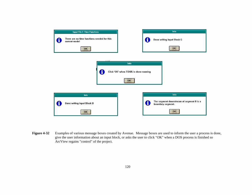
120

Figure 4-32 Examples of various message boxes created by Avenue. Message boxes are used to inform the user a process is done,give the user information about an input block, or asks the user to click "OK" when a DOS process is finished soArcView regains "control" of the project.

121

• If parameters are changed in the tables, all input blocks which are affected by those

characteristics that have been modified are rerun. For example, if cross sectional

areas are changed , it is necessary to rerun both Input Block B: Exchanges, and

Input Block C: Volumes, since the cross sectional area is used in both of these

blocks.

Most of the input block creation process reads information from the tables outlined in

Section 4.6.4. To change information in a within a table in ArcView, the table must be in a dbf

format. Since ArcView only allows one to modify dbf tables, if an INFO file needs to be

changed, it is first exported out of ArcView as a dbf file, reopened into the project, and

renamed to the correct name. Once the table is a dbf file, it is changed by following the steps

below:

1. To edit the table, make it active and choose Table: Start Editing on the menu bar

(see Figure 4-33). Then, choose the editing icon from the tool bar and change the

values. When complete, select Table: Stop Editing from the menu.

2. Set the project window active and select BOD/DO Model from the menu bar. A

menu appears, displaying all ten input blocks (Figure 4-30). Choose the input

block to recreate and Avenue regenerates the necessary text files.

3. Rerun Input Block A in order to rename the WASP5 input file and preserve the

previous input file (if desired).

4. When complete, choose BOD/DO Model: Generate Input File, to recreate the input

file with the new information.

Dry Weather Conditions

For the BOD/DO model input file, the user has the option to simulate "dry weather"

conditions. During the generation of Input Blocks D and F, Avenue prompts the user to

simulate average or dry weather flows. If "dry weather conditions" is chosen, the input file will

have just baseflow conditions and point source loads only. It is important that the answer to the

query at each input block is consistent; otherwise, an inaccurate input file which either

discludes runoff flows or non-point source loads is created.

122

Table edit icon located on lower tool bar

Figure 4-33 ArcView menu showing option to Start Editing. Once chosen, the table edit icon (above) is highlighted and the selectedtable (in this case, "Boundary Segments") is changed. Only dBase tables can be edited.

123

Calibration Input File

Before running the BOD/DO model in EUTRO5, the system being modeled must first

be calibrated. The user can perform this calibration without the help of the ArcView

connection, or utilize the ArcView to assist in the model calibration. For calibration, the

TOXI5 is used to model a conservative substance in the system. Typically, at least two

boundary conditions are set to a known concentration value of the substance; the rest of the

segments are set to initial conditions of 0. The model is run and once equilibrium in the

system is reached, the calculated values of the conservative substance are compared to known

values.

For the calibration in this connection, the method employed is a steady state model

using TOXI5, level one complexity and salinity as the conservative substance. When the menu

choice Write Input Information under Model Calibration is chosen (see Figure 4-25), Avenue

reads the data from the tables. In addition, the model constants and the desired segment

numbers set as the boundary conditions are input by the user. As in the regular input file

generation, the Avenue program creates 13 text files. A number of these files are identical to

the blocks needed for a BOD/DO model run; specifically, input blocks B,C,D, and I. For this

reason, the same free form text files (b.txt,c.txt,d.txt, and i.txt) are written to the working

directory. For all other input blocks, the free form text files have the prefix "cal" (i.e. cala.txt).

An Overview of Each Input Block

As mentioned earlier, WASP5 requires 10 input blocks for a completely formatted

input file. Most of the information for each one of these input blocks is read by Avenue, using

the corresponding choices on the menu bar (see Figure 4-25). However, some defaults to each

input block were set within the input block creation in order to make writing the formatted input

file more efficient and easier. The following is a short description of each information read

from ArcView for each input block and the defaults that were set in its generation.

124

Input Block A: Model Identification and Simulation Control

This input block contains basic simulation information and model preferences. The

script reads how many segments are present and queries the user to choose model preferences

such as length of model run, preferred time step, and print intervals. This script also asks for a

model title, which is printed on the first line of the input file, and the input file name (*.inp).

This file name uses the standard DOS 8.3 file naming convention and always has the extension

".inp".

The following defaults are set in the generation of this input block:

• Presently, the connection is set to handle just EUTRO5 for Simple Street-Phelps

modeling and level one complexity TOXI5 for calibration.

• Backward differencing is always used.

• A transport file is always generated.

• The first six segments' solutions are those which are displayed on the screen, during

a model run.

• The same maximum time step is used throughout the model run.

• The same print interval is used throughout the model run.

Input Block B: Exchange Coefficients

This input block describes the exchange coefficients for surface water (pore water

exchanges are not set in the connection). The script reads the lengths of the segments to

calculate the characteristic length between segments. It also determines if the boundary

segments are perpendicular to the main segmentation and compensates for that attribute in the

characteristic length. Finally, it reads the exchange coefficients and cross-sectional areas for

two neighboring segments and chooses the smaller area and the exchange coefficient for printing

to the text file. It also established the exchange between the benthic sediment and the water

column to emulate a possible sink or source for DO.

The following defaults are set:

125

• Exchange coefficients are steady-state.

• Exchange coefficients are written to the text file in m2/sec and lengths are in m.

Input Block C: Volumes

This input block describes the segment volumes for the system. It also sets the

hydraulic geometry parameters for calculating segment depth and velocity. These geometry

parameters are used to calculate reaeration (if necessary) or volatilization from the segments;

they are not used in transport calculations (Ambrose, et al., 1993). For this connection, a

constant (in time and space) reaeration coefficient has been assumed; therefore, these geometry

parameters are not used to calculate reaeration in this particular set up. The script reads the

cross-sectional areas (m2) and multiplies it by that segment's length (m) to obtain the volume.

The script also asks the user to choose the following: 1) water column volume option, 2)

benthic volume option, and 3) benthic time step.

The following defaults are set:

• Volumes are written to the text file in m3.

• Geometry parameters do not spatially vary.

• Only the first benthic volume option is possible.

Input Block D: Flows

This input block provides the advective transport flows that are used in the model.

Presently, only flows for WASP5 Flow Field 1 (water column) are used in the connection.

First, the script asks the user to choose a flow option. These options are described below

(Ambrose, et al., 1993):

1. Field one flows are specified directly by the user. Individual flows at each

segment interface are summed by the model, and the net flow us applied across the

interface.

2. Field one flows are specified directly by the user. Individual flows at each

segment interface are applied directly by the model.

126

3. Flows are read from a formatted file created by DYNHYD5 or another

hydrodynamic model. If this option is chosen, the user is asked to enter the file

name of the text file which hold this information.

The table, "flow.dbf" (Figure 4-34) is created during this input block determination, by

doing a units conversion on the "Flow Accumulation Values" and the Runoff Accumulation

Values tables (Figure 4-26) (mm/yr/ha to m3/sec). This table gives the total cumulative flow,

incremental flow, runoff, and baseflow into each main segment in m3/sec. The baseflow is

found by subtracting the incremental runoff from the incremental flow.

The script in ArcView assumes that each boundary segment given has an associated

flow and each main segment has just one flow input. The script tracks each flow input from its

upper-most boundary to the most downstream segment (see Figure 4-22). To do this process,

each boundary segment and its corresponding upstream and downstream segments are read from

the "Boundary Segments" table. The main segment, which is downstream of a given boundary,

is then found in the "Main Segmentation" table, and its corresponding downstream segment is

obtained. The script continues to look for the successive downstream segments, until the most

downstream main segment is reached. This flow route is printed to the text file and, at the end

of the flow path, the actual flow from the original boundary segment is printed. If dry weather

conditions are chosen, Avenue replaces the total flow in this text file with just the baseflow.

The following defaults are set:

• All flows are in m3/sec. The percentages of the total flow are written to the text

file, along with the total flow value.

• The flow is steady state.

• The number of flow fields is set to 1: water column only (no pore water flows).

127

Figure 4-34 The two dbf files which are created during the BOD/DO input block execution.Flow.dbf gives the cumulative flow, incremental flow, runoff, and baseflow foreach segment in m3/sec, while load.dbf shows the point source BOD loadingand NPS BOD and DO loading into each segment in kg/day.

128

Input Block E: Boundaries

This input block describes the boundary segments and their concentrations. Model

boundaries consist of those segments that import, export, or exchange water with locations

outside the main network. A boundary is either a tributary inflow, a downstream outflow, or an

open water end of the model network across which dispersive mixing can occur. The boundary

concentrations are read from the "Boundary Segments" table.

The following defaults are set:

• Since the EUTRO5 model is set just for the Simple Streeter-Phelps Model, only

BOD and DO are considered in the boundary concentrations.

• For the calibration model, those boundary segments chosen by the user are set to

their respective salinity values, while all other boundaries are set to 0.

• All concentrations are read and written in units of mg/L.

• The boundary conditions are steady state.

Input Block F: Waste Loads

This Input Block writes the BOD and DO loads into each main network segment. The

script does two things:

1. Reads the point source BOD loads into each segment (in 103 lbs/yr) from the "Point

Source BOD" table and converts the value to kg/day.

2. Calculates the non-point source BOD from the "BOD Loading Values" table

(Figure 4-26) in kg/day by taking each load value and subtracting the previous

segment's load value to get the incremental loading to each segment.

Since the model is set for steady state, the non-point BOD loads are added to the point source

BOD loads to get a total load to the segment. This input block also generates a

table called "load.dbf" (Figure 4-34), which gives the non-point source loads in kg/day for BOD

and DO. This table also gives the total point source BOD loading in kg/day for each main

segment. If dry weather conditions is selected during this input block creation, only the

129

point source loads are written to the input file, since there is no runoff to carry the NPS loads.

The following defaults are set:

• All loads are steady state.

• Only BOD and DO are considered.

Input Block G: Parameters

This input block reads the necessary parameters for the level one EUTRO5 or level

one TOXI5 models. As the complexity level increases, the number of parameters needed also

increases. Presently, no parameters are needed for the level one TOXI5 model and only four

parameters are required for EUTRO5 level one:

1. Temperature, read from the segment tables in °C; temperature is used to correct for

deviations from the standard (20°C) and DO saturation.

2. Sediment oxygen demand (SOD), read from the tables in g/m2/day.

3. SOD theta correction, input by user; used to correct SOD for temperatures

deviating from 20°C.

4. Salinity, read from the tables; used to calculated DO saturation.

The following defaults are set:

• Temperature does not vary in time.

• SOD theta does not vary in time or space.

Input Block H: Constants

This Input Block queries the user for the necessary constants needed to run the Simple

Streeter-Phelps or the calibration models. The definition of the constants varies, depending

upon the structure and kinetics of the systems comprising each model. For the present

BOD/DO model, only two constants are needed:

1. CBOD deoxygenation rate at 20°C, per day.

2. Reaeration rate constant at 20°C for entire water body, per day.

130

For the calibration model, three constants are necessary:

1. Molecular weight of the substance being modeled in g/mol.

2. Constant partition coefficient for sorption to solids in L/kg.

3. Water column biodegradation.

The following default is set:

• The constants do not vary in time or space.

Input Block I: Time Functions

If the model were non-steady state for any parameter, this input block would use time

functions to vary the specific parameter. Presently, none of the parameters are set to vary in

time, so the default for this block is set to 0.

Input Block J: Initial Conditions

This input block describes the initial conditions for each system in the model. For the

EUTRO5 model, only DO and BOD are considered in this script. The initial conditions are

read from the segment tables. The TOXI5 model only needs to set the boundary segments that

are chosen by the user to their respective salinities, while all other initial conditions (i.e.,

salinities) are equal to zero.

The following defaults are set:

• The dissolved fraction of BOD is set at 0.5.

• The dissolved fraction of DO is always 1.0.

• The dissolved fraction for salinity is 1.0.

• The maximum value for all systems in EUTRO5 is 1.0e8.

• The maximum value for salinity is 35,000 mg/L (sea water).

• Solids Field 3 transports BOD is its particulate form.

• Solids Field 5 transports DO.

• Solids Field 3 transports NaCl.

131

• All densities are set to 1.0 (EUTRO does not use those values).

• All initial conditions are in mg/L.

4.6.7 Running the Model from ArcView

As mentioned before, the input file which is created has some limitations. This initial

connection, although quite simplified for WASP5 capabilities, can be enhanced to eliminate

some of the preset defaults presently in the code. However, at this time, this model connection

has the following limitations:

• Only steady state input files are run.

• The connection is best set up for a river system, or a tidally influenced river

system

• The Simple Streeter-Phelps Model is the complexity level -- the connection

considers just Biochemical Oxygen Demand (BOD) and Dissolved Oxygen (DO)

• Only the water column flow is considered in this connection. The connection is not

presently set up for two-layer water systems or for sediment transport.

Once an input file is created in ArcView, a model run can be executed by simply

choosing BOD/DO Model: Run EUTRO5. Be sure that the input file has been generated before

performing this step. When the model is executed, a DOS window appears and the EUTRO5

interface is shown. When a list of input files is displayed, the input file to run is executed. Do

not press the "OK" button on the message box (Figure 4-32) until the model has completed

executing. Pressing "OK" informs ArcView that the model is completely done running and

Avenue can now exit from DOS and return to the ArcView interface. In addition, the EUTRO5

or TOXI5 models do not have to be executed through ArcView. It is possible to get ArcView

to write several input files for these models and then run the model separately, through DOS,

for each file. The final output can then be processed and viewed through ArcView.

132

4.6.8 Output File Processing

There are three main steps that need to be executed in succession in order to process

and view the output from a model run:

1. Checking the model parameters

2. Processing the output file

3. Viewing the output

All of these steps can be executed from either the BOD/DO Model menu or the Calibration

Model menu. Be sure to choose the correct menu, corresponding to the model that is being

processed (see Figure 4-25).

Step 1: Checking the model parameters

This item just reinitializes the model options and file information for ArcView to

process the output. With this option, it is possible to create a number of output files with

numerous model runs and then process them, one at a time, without having to go back and rerun

the model. The correct output file name for the desired model run is input during this step. If

an output file from the calibration model is being processed, the output file is named the same

as its assigned input file name, with a ".tdf" extension. The BOD/DO model follows the same

convention, with an ".edf" extension. This step is always executed before processing and

viewing an output file.

Step 2: Processing the output file

This option executes a FORTRAN program which writes a text file with either salinity,

or BOD and DO measurements, for every segment at each time step. The text file is then

imported into ArcView as a dBase table. Avenue prompts the user to name each table, as it is

processed. If a number of output files are being processed at once, their related tables are

given descriptive names so that they can be differentiated in the project.

Step 3: Viewing the output

The first step that the user must do, after executing this command is to choose a table

to which Avenue links the newly created charts and coverages. Although the table choice

133

box displays a list of all available tables (Figure 4-35), only those that were created by the

above process step can be viewed using this menu option. If a table is chosen that does not

have the proper format, ArcView exits out of the view output script. The table selected has to

correspond to the parameters set in Step 1, above. If it does not, the user must go back and

reset the parameters correctly. This need is because the output viewing steps (such as

coverage creation) use some of these parameters in order to execute various Avenue script

commands.

Within this step, there are five options. They are as follows:

1. View the table

2. Create a chart of concentration vs. time for a chosen segment

3. Create a chart of concentration vs. segment number for a chosen time

4. Create a coverage of the concentration at the last time step in the table

5. Create a "movie" of four coverages which display concentration at four chosen

times

All charts which are created are always "linked" to a given table. If changes are made

to that table or to the selections within the table, the chart changes accordingly. For example, if

a chart of concentration vs. segment at time = 10 days has been created and another chart of

concentration vs. segment at time = 19 days is created and linked to the same table, the first

chart changes to reflect the new time. To avoid this problem, the user can create or add

multiple copies of the same table to the project and link a chart to each table. This process is

accomplished by either adding the dbf file numerous times and renaming the table so that it is

more descriptive or processing the same output a number of times and

changing the table name when prompted for a name. Then, only one chart is linked to each

table and the charts remains independent of one another.

Option 1: Viewing the Table (Figure 4-36)

By choosing this option, the selected table opens and become the active view. The

user can then view the output or create charts manually from this table, if desired.

134

(a)

(b)

Figure 4-35 Query boxes: (a) shows the list of tables to choose from which new charts andthemes are created and (b) displays the output options available to the user.Only those tables with a "Time" field are able to be processed.

135

Figure 4-36 Table (dbf format) which is created during the output file processing of the WASP5 output. This table shows values ofsalinity (in ppt) and is opened when the first choice for the output presentation is chosen.

136

Option 2: Concentration vs. Time (Figure 4-37)

This option opens the view, "Segmentation" (Figure 4-29) and prompt the user to

activate the "bug" icon and choose a segment. Once the "bug" icon located on the far right

bottom tool bar is active, the proper theme (either Main Segmentation or Boundary

Segmentation) is highlighted. The chart is created by clicking on the segment to graph. The

user is asked a few chart options, including color and the name of the y-axis. Afterwards, a

chart, showing concentration vs time ( for all time steps) appears.

Option 3: Concentration vs. Segment Number (Figure 4-38)

This option prompts the user for the time at which to display the concentration values.

A bar chart showing the concentration for each segment (main and boundary) is then created. If

a different time is desired, the new time is selected on the linked table and the chart changes to

reflect the new selection.

Option 4: Coverage at Final Time (Figure 4-39)

This option creates an ArcView coverage of the concentration at the final time in the

model run. The script automatically brings the coverage up on the view, "Segmentation", and

shows the concentration values for that time, in a ramped arc coverage (from blue to red).

Option 5: Movie of Four Chosen Times (Figure 4-40)

This option allows the user to choose four given times from all possible times in a

chosen table. The script then opens the view, "Segmentation", and creates a coverage, at a

chosen time delay. The script determines the minimum and maximum values within the

selected times and ramp the coverage from gray to blue in eight intervals. These intervals stays

constant for all four times, so that changes in concentrations can be viewed consistently. After

the script is complete, the user has four new coverages of concentration at each time step.

137

Figure 4-37 Result of second choice in output file presentation options: chart of concentration vs. time for a given segment andchosen table. The chart is created by choosing the bug icon from the view toolbar (see Figure 4-26) and choosing thesegment off of the view to chart.

138

Figure 4-38 Query box and chart for third output presentation option: concentration vs.segment number at a chosen time. The query box allows the user to pick thetime at which to chart the concentrations. Segment #9 is the benthic sedimentlayer; no salinity is modeled in that segment.

139

Figure 4-39 New theme created by fourth output presentation option. This new theme shows concentration at the last time in themodel run. The arcs are ramped from blue to red.

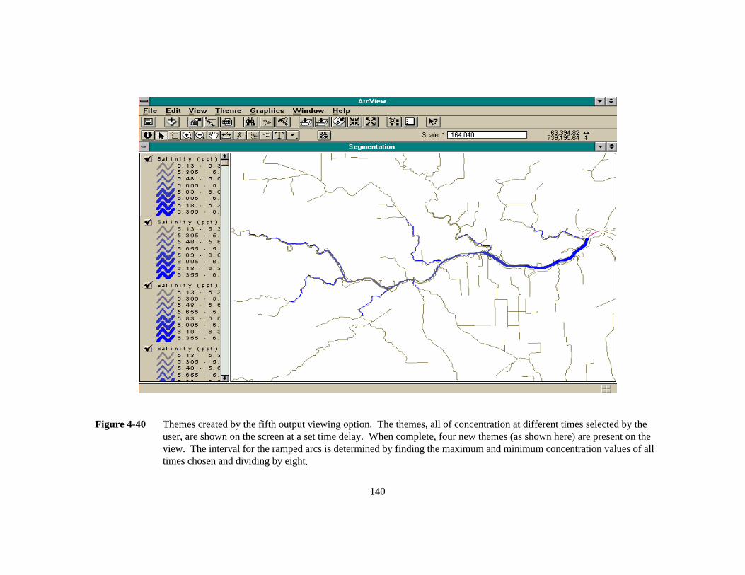
140

Figure 4-40 Themes created by the fifth output viewing option. The themes, all of concentration at different times selected by theuser, are shown on the screen at a set time delay. When complete, four new themes (as shown here) are present on theview. The interval for the ramped arcs is determined by finding the maximum and minimum concentration values of alltimes chosen and dividing by eight.

141

4.6.9 Help File Creation

Located within this customized project is a "help" document to assist a user in the use

of this model connection. To activate this help document, the option Help on WASP5/ArcView

Connection under Help on the menu bar is chosen (Figure 4-41). This file is a hypertext

document, compiled in rich text format and executed under Windows's help file (winhelp.exe).

This help document, shown in Appendix G, gives information on the model, the connection, the

input blocks, troubleshooting, limitations, and references. In addition, it outlines how to create

an initial input file, to change an input block, to run the model, and to perform a model

calibration.

4.6.10 Setting up the WASP5/ArcView Connection

The ArcView/WASP5 model connection and a demo which shows the Houston Ship

Channel study discussed in this report can be set up on any computer which has ArcView 2.1

or higher installed on the machine. In order to set up the demonstration on a personal computer,

the following steps are taken:

• Install WASP5 onto the computer. WASP5 is available from the USEPA Homepage

(ftp://ftp.epa.gov/epa_ceam/wwwhtml/wasp.htm).

• Download the demonstration files, in zipped format, from the University of Texas,

Center for Research in Water Resources Homepage for the ArcView/WASP5

connection demo (http://www.ce.utexas.edu/prof/maidment /GISHydro/) and unzip them

into the directory that the WASP5 executables are located.

• Open the project hsc_wasp.apr in ArcView version 2.1 or higher. ArcView may

initially ask the user to location of some coverages and tables. All necessary

coverages and tables should be located with in the directory in which the downloaded

file was unzipped. Most tables are in dbf format, while the coverages are in a folder

entitled cover.

142

Figure 4-41 Windows help document run by winhelp.exe and created to assist a user in theexecution of the WASP5/ArcView connection.

143

• Open the script vwout and locate the two references to the arc coverage segarc. Both

of the lines in the script read:

• segSrcName = SrcName.Make("c:\wasp\cover\segarc arc")

• This line informs Avenue on where to locate the main segmentation coverage. Be sure

that the drive and directory name in this line is correct. Also, if this script is being

recompiled for a new system, this line should reference the correct location and name

for the main segmentation coverage in the new system that has been developed.

• If the vwout script was changed, in any way, recompile it, by clicking on the checkmark

icon on the bottom toolbar of the ArcView script tools.

• Model input file creation, model runs, and output viewing can then be performed as

described previously in this section.