Chapter 4

Numerical Integration

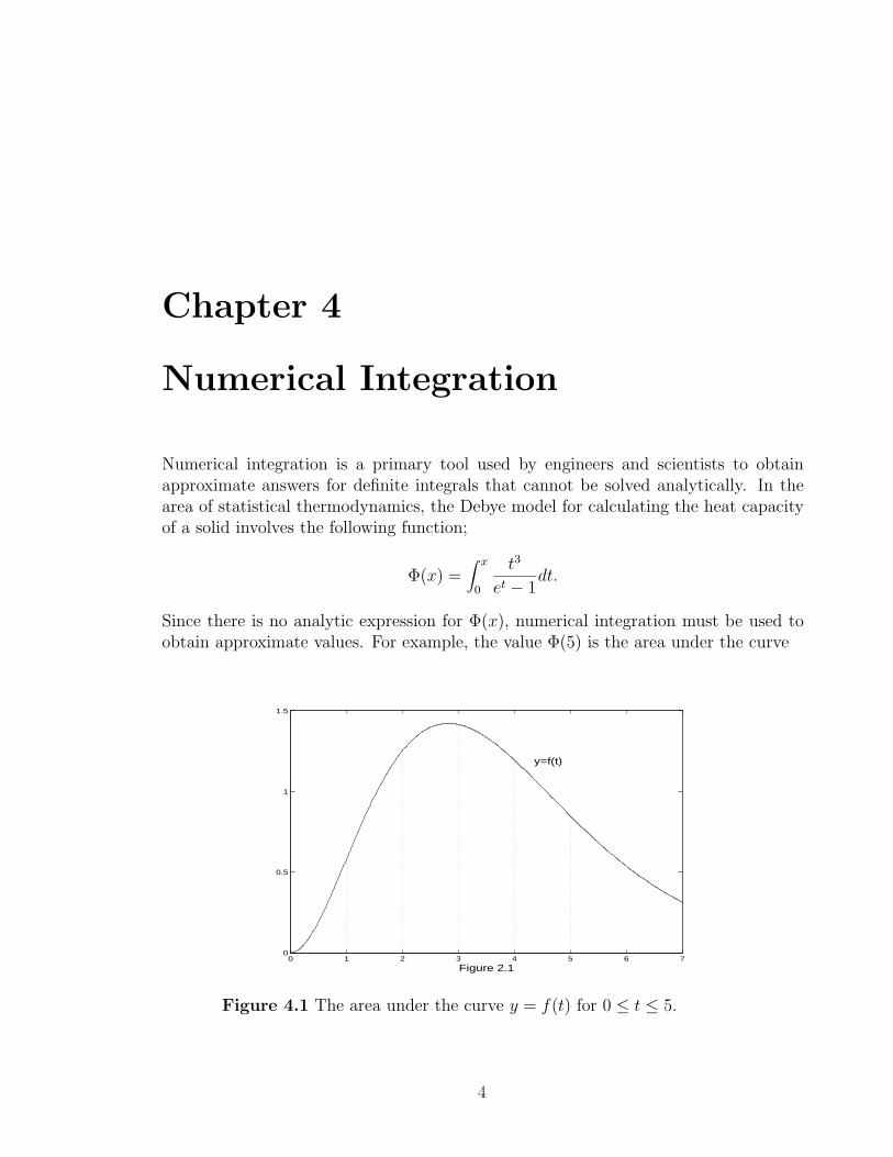
Numerical integration is a primary tool used by engineers and scientists to obtainapproximate answers for definite integrals that cannot be solved analytically. In thearea of statistical thermodynamics, the Debye model for calculating the heat capacityof a solid involves the following function;

Φ(x) =∫ x

0

t3

et − 1dt.

Since there is no analytic expression for Φ(x), numerical integration must be used toobtain approximate values. For example, the value Φ(5) is the area under the curve

0 1 2 3 4 5 6 70

0.5

1

1.5

Figure 2.1

y=f(t)

Figure 4.1 The area under the curve y = f(t) for 0 ≤ t ≤ 5.

4

Figure 4.1 Values of Φ(x)

x Φ(x)1.0 0.22480522.0 1.17634263.0 2.55221854.0 3.87705425.0 4.89989226.0 5.58585547.0 6.00316908.0 6.23962389.0 6.366573910.0 6.4319219

y = f(t) = t3/(et− 1) for 0 ≤ t ≤ 5 (see Figure 4.1). The numerical approximation forΦ(5) is

Φ(5) =∫ 5

0

t3

et − 1dt ≈ 4.8998922.

Each additional value of Φ(x) must be determined by another numerical integration.Table 4.1 lists several of these approximations over the interval [1, 10].

The purpose of this chapter is to develop the basic principles of numerical integra-tion. In Chapter 9, numerical integration formulas are used to derive the predictor-corrector methods for solving differential equations.

4.1 Introduction to Quadrature

We now approach the subject of numerical integration. The goal is to approximate thedefinite integral of f(x) over the interval [a, b] by evaluating f(x) at a finite number ofsample points.

Definition 4.1 Suppose that a = x0 < x1 < · · · < xM = b. A formula of theform

Q[f ] =M∑

k=0

wkf(xk) = w0f(x0) + w1f(x1) + · · ·+ wMf(xM) (4.1)

with the property that ∫ b

af(x)dx = Q[f ] + E[f ] (4.2)

5

is called a numerical integration or quadrature formula. The term E(f) is calledthe truncation error for integration. The values {xk}M

k=0 are called the quadraturenodes, and {wk}M

k=0 are called the weights .

Depending on the application, the nodes {xk} are chosen in various ways. For thetrapezoidal rule, Simpson’s rule, and Boole’s rule, the nodes are chosen to be equallyspaced. For Gauss-Legendre quadrature, the nodes are chosen to be zeros of certainLegendre polynomials. When the integration formula is used to develop a predictorformula for differential equations, all the nodes are chosen less than b. For all applica-tion, it is necessary to know something about the accuracy of the numerical solution.

Definition 4.2. The degree of precision of a quadrature formula is the positiveinteger n such that E[Pi] = 0 for all polynomials Pi(x) of degree i ≤ n, but for whichE[Pn+1] 6= 0 for some polynomial Pn+1(x) of degree n + 1.

The form of E[Pi] can be anticipated by studying what happens when f(x) is apolynomial. Consider the arbitrary polynomial

Pi(x) = aixi + xi−1x

i−1 + · · ·+ a1x + a0

of degree i. If i ≤ n, then P(n+1)i (x) ≡ 0 for all x, and P

(n+1)n+1 (x) = (n + 1)!an−1 for all

x. Thus it is not surprising that the general form for the truncation error term is

E[f ] = Kf (n+1)(c), (4.3)

where K is a suitably chosen constant and n is the degree of precision. The proof ofthis general result can be found in advanced books on numerical integration.

The derivation of quadrature formulas is sometimes based on polynomial interpo-lation. Recall that there exists a unique polynomial PM(x) of degree ≤ M passingthrough the M + 1 equally spaced points {(xk, yk)}M

k=0. When this polynomial is usedto approximate f(x), over [a, b], and then the integral of f(x) is approximated bythe integral of PM(x), the resulting formula is called a Newton-Cotes quadratureformula (see Figure 2.2). When the sample points x0 = a and xM = b are used,itis called a closed Newton-Cotes formula. The next result gives the formulas whenapproximating polynomials of degree M = 1, 2, 3, and 4 are used.

Theorem 4.1 (Closed Newton-Cotes Quadrature Formula). Assume that xk =x0 + kh are equally spaced nodes and fk = f(xk). The first four closed Newton-Cotes

6

quadrature formulas are

∫ x1

x0

f(x)dx ≈ h

2(f0 + f1) (the traezoidal rule), (4.4)

∫ x2

x0

f(x)dx ≈ h

3(f0 + 4f1 + f2) (Simpson’s rule), (4.5)

∫ x3

x0

f(x)dx ≈ 3h

8(f0 + 3f1 + 3f2 + f3) (Simpson’s 3

8rule), (4.6)

∫ x4

x0

f(x)dx ≈ 2h

45(7f0 + 32f1 + 12f2 + 32f3 + 7f4) (Boole’s rule). (4.7)

Figure 2.2 (a) The trapezoidal rule integrates (b) Simpson’s rule integrates (c) Simp-son’s rule integrates (d) Boole’s rule integrates

Corollary 4.1 (Newton-Cotes Precision). Assume that f(x) is sufficiently dif-ferentiable; then E[f ] for Newton-Cotes quadrature involves an appropriate higherderivative. The trapezoidal rule has degree of precision n = 1. If f ∈ C2[a, b], then

∫ x1

x0

f(x)dx =h

2(f0 + f1)− h3

12f (2)(c). (4.8)

7

Simpson’s rule has degree of precision n = 3. If f ∈ C4[a, b], then

∫ x2

x0

f(x) =h

3(f0 + 4f1 + f2)− h5

90f (4)(c). (4.9)

Simpson’s 38

rule has degree of precisionn = 3. If f ∈ C4[a, b], then

∫ x3

x0

f(x)dx =3h

8(f0 + 3f1 + 3f2 + f3)− 3h5

80f (4)(c). (4.10)

Boole’s rule has degree of precision n = 5, If f ∈ C6[a, b], then

∫ x4

x0

f(x)dx =2h

45(7f0 + 32f1 + 12f2 + 32f3 + 7f4)− 8h7

945f (6)(c). (4.11)

Proof of Theorem 4.1. Start with the Lagrange polynomial PM(x) based on x0, x1, . . . , xM

that can be used to approximate f(x):

f(x) ≈ PM(x) =M∑

k=0

fkLM,k(x), (4.12)

where fk = f(xk) for k = 0, 1, . . . , M. An approximation for the integral is obtained byreplacing the integrand f(x) with the polynomial PM(x). This is the general methodfor obtaining a Newton-Cotes integration formula:

∫ xM

x0

f(x) ≈∫ xM

x0

PM(x)dx

=∫ xM

x0

(M∑

k=0

fkLM,k(x)

)dx =

M∑

k=0

(∫ xM

x0

fkLM,k(x)dx)

(4.13)

=M∑

k=0

(∫ xM

x0

LM,k(x)dx)

fk =M∑

k=0

wkfk.

The details for the general computations of coefficients of wk in (4.13) are tedious. Weshall give a sample proof of Simpson’s rule, which is the case M = 2. This case involvesthe approximating polynomial

P2(x) = f0(x− x1)(x− x2)

(x0 − x1)(x0 − x2)+ f1

(x− x0)(x− x2)

(x− x0)(x− x2)+ f2

(x− x0)(x− x1)

(x2 − x0)(x2 − x1). (4.14)

8

Since f0, f1, and f2 are constants with respect to integration, the relations in (4.13)lead to

∫ x2

x0

f(x)dx ≈ f0

∫ x2

x0

(x− x1)(x− x2)

(x0 − x1)(x0 − x2)dx (4.15)

+f1

∫ x2

x0

(x− x0)(x− x2)

(x1 − x0)(x1 − x2)dx + f2

∫ x2

x0

(x− x0)(x− x1)

(x2 − x0)(x2 − x1)dx

We introduce the change of variable x = x0 + ht with dx = hdt to assist with theevaluation of the integrals in (4.15). The new limits of integration are from t = 0 tot = 2. The equal spacing of the nodes xk = x0 + kh leads to xk − xj = (k − j)h andx− xk = h(t− k), which are used to simplify (4.15) and get

∫ x2

x0

f(x)dx ≈ f0

∫ 2

0

h(t− 1)h(t− 2)

(−h)(−2h)hdt + f1

∫ 2

0

h(t− 0)h(t− 2)

(h)(−h)hdt (4.16)

+f2

∫ 2

0

h(t− 0)h(t− 1)

(2h)(h)hdt

= f0h

2

∫ 2

0(t2 − 3t + 2)dt− f1h

∫ 2

0(t2 − 2t)dt + f2

h

2

∫ 2

0(t2 − t)dt

= f0h

2

(t3

3− 3t2

2+ 2t

) ∣∣∣t=2

t=0− f1h

(t3

3− t2

) ∣∣∣t=2

t=0

+f2h

2

(t3

3− t2

2

) ∣∣∣t=2

t=0

= f0h

2

(2

3

)− f1h

(−4

3

)+ f2

h

2

(2

3

)

=h

3(f0 + 4f1 + f2).

and the proof is complete. We postpone a sample proof of Corollary 4.1 until Section4.2.

Example 2.1. Consider the function f(x) = 1+e−x sin(4x), the equally spaced spacedquadrature nodes x0 = 0.0, x1 = 0.5, x2 = 1.0, x3 = 1.5, and x4 = 2.0, and the corre-sponding function values f0 = 1.00000, f2 = 0.72159, f3 = 0.93765, and f4 = 1.13390.Apply the various quadrature formulas (2.4) through (2.7).

9

The step size is h = 0.5, and the computations are∫ 0.5

0f(x)dx ≈ 0.5

2(1.00000 + 1.55152) = 0.63788

∫ 1.0

0f(x)dx ≈ 0.5

3(1.00000 + 4(1.55152) + 0.72159) = 1.32128

∫ 1.5

0f(x)dx ≈ 3(0.5)

8(1.00000 + 3(1.55152) + 3(0.72159) + 0.93765)

= 1.64193∫ 2.0

0f(x)dx ≈ 2(0.5)

45(7(1.00000) + 32(1.55152) + 12(0.72159)

+32(0.93765) + 7(1.13390)) = 1.29444.

It is important to realize that the quadrature formulas (4.4) through (4.7) applied inthe above illustration give approximations for definite integrals over different intervals.The graph of the curve y = f(x) and the areas under the Lagrange polynomials y =P1(x), y = P2(x), y = P3(x), and P4(x) are shown in Figure 4.2 (a) through (d),respectively.

In Example 4.1 we applied the quadrature rules with h = 0.5. If the endpointsof the interval [a, b] are held fixed, the step size must be adjusted for each rule. Thestep sizes are h = b − a, h = (b − a)/2, h = (b − a)/3, and h = (b − a)/4 for thetrapezoidal rule, Simpson’s rule, Simpson’s 3

8rule, and Boole’s rule, respectively. The

next example illustrates this point.

Example 2.2 Consider the integration of the function f(x) = 1 + e−x sin(4x) overthe fixed interval [a, b] = [0, 1]. Apply the various formulas (4.4) through (4.7).

For the trapezoidal rule, h = 1 and∫ 1

0f(x)dx ≈ 1

2(f(0) + f(1))

=1

2(1.00000 + 0.72159) = 0.86079.

For Simpson’s rule, h = 1/2, we get

∫ 1

0f(x)dx ≈ 1/2

3(f(0) + 4f(1/2) + f(1))

=1

6(1.00000 + 4(1.55152) + 0.72159) = 1.32128.

For Simpson’s 38

rule, h = 1/3, and we obtain

∫ 1

0f(x)dx ≈ 3(1/3)

8(f(0) + 3f(

1

3) + 3f(

2

3) + f(1))

10

=1

8(1.00000 + 3(1.69642) + 3(1.23447) + 0.72159) = 1.31440.

For Boole’s rule, h = 1/4, and the result is

∫ 1

0f(x)dx ≈ 2(1/4)

45(7f(0) + 32f(

1

4) + 12f(

1

2) + 32f(

3

4) + 7f(1))

=1

90

(7(1.00000) + 32(1.65534) + 12(1.55152)

+32(1.06666) + 7(0.72159))

= 1.30859.

The true value of the definite integral is

∫ 1

0f(x)dx =

21e− 4 cos(4)− sin(4)

17e= 1.3082506046426 . . . ,

and the approximation 1.30859 from Boole’s rule is best, the area under each of theLagrange polynomials P1(x), P2(x), P3(x), and P4(x) is shown in Figure 2.3(a) through(d), respectively.

Figure 2.3 (a) the trapezoidal rule used over [0,1] yields the approximation 0.86079(b) simpson’s rule used over [0,1] yields the approximation 1.32128. (c) simpson’s ruleused over [0,1] yields the approximation 1.31440. [d] boole’s rule used over [0,1] yieldsthe approximation 1.30859.

To make a fair comparison of quadrature methods, we must use the same number offunction evaluations in each method. Our final example is concerned with comparingintegration over a fixed interval [a, b] using exactly five function evaluations fk = f(xk),for k = 0, 1, . . . , 4 for each method. When the trapezoidal rule is applied on the foursubintervals [x0, x1], [x1, x2], x2, x3], and [x3, x4], it is called a composite trapezoidalrule :

∫ x4

x0

f(x)dx =∫ x1

x0

f(x)dx +∫ x2

x1

f(x)dx +∫ x3

x2

f(x)dx +∫ x4

x3

f(x)dx

≈ h

2(f0 + f1) +

h

2(f1 + f2) +

h

2(f2 + f3) +

h

2(f3 + f4) (4.17)

=h

2(f0 + 2f1 + 2f2 + 2f3 + f4).

Simpson’s rule can also be used in this manner. When Simpson’s rule is applied on thetwo subintervals [x0, x2] and [x2, x4], it is called a composite Simpson’s rule :

∫ x4

x0

f(x)dx =∫ x2

x0

f(x)dx +∫ x4

x2

f(x)dx

≈ h

3(f0 + 4f1 + f2) +

h

3(f2 + 4f3 + f4) (4.18)

11

=h

3(f0 + 4f1 + 2f2 + 4f3 + f4)

The next example compares the values obtained with (2.17), (2.18), and(2.7).

Example 2.3. Consider the integration of the function f(x) = 1 + e−x sin(4x) over[a, b] = [0, 1]. Use exactly five function evaluations and compare the results from thecomposite trapezoidal rule, composite Simpson rule, and Boole’s rule.

The uniform step size is h = 1/4. The composite trapezoidal rule (2.17) produces

∫ 1

0f(x)dx ≈ 1/4

2(f(0) + 2f(

1

4) + 2f(

1

2) + 2f(

3

4) + f(1))

=1

8(1.00000 + 2(1.65534) + 2(1.55152) + 2(1.06666) + 0.72159)

= 1.28358

Using the composite Simpson’s rule (2.18), we get

∫ 1

0f(x)dx ≈ 1/4

3(f(0) + 4f(

1

4) + 2f(

1

2) + 4f(

3

4) + f(1))

=1

12(1.00000 + 4(1.65534) + 2(1.55152) + 4(1.06666) + 0.72159)

= 1.30938

We have already seen the result of Boole’s rule in Example 7.2:

∫ 1

0f(x)dx ≈ 2(1/4)

45(7f(0) + 32f(

1

4) + 12f(

1

2) + 32f(

3

4) + 7f(1))

= 1.30859.

Figure 2.4 (a) the composite trapezoidal rule yields the approximation 1.28358. (b)the composite simpson rule yields the approximation 1.30938.

The true value of the integral is

∫ 1

0f(x)dx =

21e− 4 cos(4)− sin(4)

17e= 1.30825046426 . . . ,

and the approximation 1.30938 from Simpson’s rule is much better than the value1.28358 obtained from the trapezoidal rule. Again, the approximation 1.30859 fromBoole’s rule is closest. Graphs for the areas under the trapezoids and parabolas areshown in Figure 2.4(a) and (b), respectively.

Example 2.4 determine the degree of precision of Simpson’s 38

rule.

12

It will suffice to apply Simpson’s 38

rule over the interval [0, 3] with the five testfunctions f(x) = 1, x, x2, x3 and x4. For the first four functions, Simpson’s 3

8rule is

exact. ∫ 3

01dx = 3 =

3

8(1 + 3(1) + 3(1) + 1)

∫ 3

0xdx =

9

2=

3

8(0 + 3(1) + 3(2) + 3)

∫ 3

0x2dx = 9 =

3

8(0 + 3(1) + 3(4) + 9)

∫ 3

0x3dx =

81

4=

3

8(0 + 3(1) + 3(8) + 27).

The function f(x) = x4 is the lowest power of x for which the rule is not exact.

∫ 3

0x4dx =

243

5≈ 99

2=

3

8(0 + 3(1) + 3(16) + 81).

Therefore, the degree of precision of Simpson’s 38

rule is n = 3.

4.1.1 Exercises for introduction to quadrature

1. Consider integration of f(x) over the fixed interval [a, b] = [0, 1]. Apply the variousquadrature formulas (4) through (7). The step sizes are h = 1, h = 1

2, h = 1

3, and

h = 14

for the trapezoidal rule, Simpson’s rule, Simpson’s 38

rule, and Boole’s rule,respectively.

(a) f(x) = sin(πx)(b) f(x) = 1 + e−x cos(4x)(c) f(x) = sin(

√x)

Remark. The true values of the definite integrals are (a)2/π = 0.636619772367 . . .,(b) 18e− cos(4) + 4 sin(4))/(17e) = −1.007459631397 . . ., and (c) 2(sin(1)− cos(1)) =0.602337357879 . . .. Graphs of the functions are shown in Figures 2.5(a) through (c),respectively.2. Consider integration of over the fixed interval [a, b]=[0, 1]. Apply the various quadra-ture formulas; the composite trapezoidal rule (2.17), the composite Simpson rule (2.18),and Boole’s rule (2.7). Use five function evaluations at equally spaced nodes. The uni-form step size is h = 1

4.

(a) f(x) = sin(πx)(b) f(x) = 1 + e−x cos(4x)(c) f(x) = sin(

√x)

3. Consider a general interval [a, b]. Show that Simpson’s rule produces exact resultsfor the functions f(x) = x2 and f(x) = x3; that is,

13

(a)∫ ba x2dx = b3

3− a3

3(b)

∫ ba x3dx = b4

4− a4

4

4. Integrate the Lagrange interpolation polynomial

P1(x) = f0x− x1

x0 − x1

+ f1x− x0

x1 − x0

over the interval [x0, x1] and establish the trapezoidal rule.Figure 7.55. Determine the degree of precision of the trapezoidal rule. It will suffice to apply

the trapezoidal rule over [0, 1] with the three test functions f(x) = 1, x, and x2.6. Determine the degree of precision of Simpson’s rule. It will suffice to apply Simpson’srule over [0, 2] with the five test functions f(x) = 1, x, x2, x3, and x4. Contrast yourresult with the degree of precision of Simpson’s 3

8rule.

7. Determine the degree of precision of Boole’s rule. It will suffice to apply Boole’srule over [0, 4] with the seven test functions f(x) = 1, x, x2, x3, x4, x5, and x6.8. The intervals in exercises 5, 6, and 7 and Example 2.4 were selected to simplify thecalculation of the quadrature nodes. But, on any closed interval [a, b] over which thefunction f is integrable, each of the four quadrature rules (2.4) through (2.7) has thedegree of precision determined in Exercises 5, 6, and 7 and Example 2.4, respectively.A quadrature formula on the interval [a, b] can be obtained from a quadrature formulaon the interval [c, d] by making a change of variables with the linear function

x = g(t) =b− a

d− ct +

ad− bc

d− c.

where dx = b−ad−c

dt.(a) Verify that x = g(t) is the line passing through the points (c, a) and (d, b).(b) Verify that the trapezoidal rule has the same degree of precision on the interval

[a, b] as on the interval [0, 1].(c) Verify that Simpson’s rule has the same degree of precision on the interval [a, b]

as on the interval [0, 2].(d) Verify that Simpson’s rule has the same degree of precision on the interval [a, b]

as on the interval [0, 4].9. Derive Simpson’s rule using Lagrange polynomial interpolation. Hint. After chang-ing the variable, integrals similar to those in (2.16) are obtained:

∫ x3

x0

f(x)dx ≈ −f0h

6

∫ 3

0(t− 1)(t− 2)(t− 3)dt + f1

h

2

∫ 3

0(t− 0)(t− 2)(t− 3)dt

−f2h

2

∫ 3

0(t− 0)(t− 1)(t− 3)dt + f3

h

6

∫ 3

0(t− 0)(t− 1)(t− 2)dt

= f0h

2

(t4

4+ 2t3 − 11t2

2+ 6t

) ∣∣∣t=3

t=0+ f1

h

2

(t4

4− 5t3

3+ 3t2

) ∣∣∣t=3

t=0

14

+f2h

2

(−t4

4+

4t3

3− 3t2

2

) ∣∣∣t=3

t=0+ f3

h

6

(t4

4− t3 + t2

) ∣∣∣t=3

t=0

10. Derive the closed Newton-Cotes quadrature formula, based on a Lagrange approx-imating polynomial of degree 5, using the 6 equally spaced nodes xk = x0 + kh, wherek = 0, 1, . . . , 5.11. In the proof of Theorem 2.1. Simpson’s rule was derived by integrating the second-degree Lagrange polynomial based on the three equally spaced nodes x0, x1, and x2.Derive Simpson’s rule by integrating the second-degree Newton polynomial based onthe three equally spaced nodes x0, x1, and x2.

4.2 Composite Trapezoidal and Sinpson’s Rule

An intuitive method of finding the area under the curve y = f(x) over [a, b] is by approx-imating that area with a series of trapezoids that lie above the intervals {[xk, xk+1]}.

Theorem 2.2 (Composite Trapezoidal Rule). Suppose that the interval [a, b]is subdivided into M subintervals [xk, xk+1] of width h = (b − a)/M by using theequally spaced nodes xk = a + kh, for k = 0, 1, . . . , M . The composite trapezoidalrule for M subintervals can be expressed in any of three equivalent ways:

T (f, h) =h

2

M∑

k=1

(f(xk−1) + f(xk)) (4.19)

or

T (f, h) =h

2(f0 + 2f1 + 2f2 + 2f3 + · · ·+ 2fM−2 + 2fM−1 + fM) (4.20)

or

T (f, h) =h

2(f(a) + f(b)) + h

M−1∑

k=1

f(xk). (4.21)

This is an approximation to the integral of f(x) over [a, b], and we write

∫ b

af(x)dx ≈ T (f, h). (4.22)

Proof. Apply the trapezoidal rule over each subinterval [xk−1, xk] (see Figure 2.6). Usethe additive property of the integral for subintervals:

∫ b

af(x)dx =

M∑

k=1

∫ xk

xk−1

f(x)dx ≈M∑

k=1

h

2(f(xk−1) + f(xk)). (4.23)

Since h/2 is a constant, the distributive law of addition can be applied to obtain (2.19).Formula (2.20) is the expanded version of (2.19). Formula (2.21) shows how to groupall the intermediate terms in (2.20) that are multiplied by 2.

15

Approximating f(x) = 2 + sin(2√

x) with piecewise linear polynomials results inplaces where the approximating is close and places where it is not. To achieve accuracythe composite trapezoidal rule must be applied with many subintervals. In the nextexample we have chosen to numerically integrate this function over the interval [1, 6].Investigation of the integral over [0, 1] is left as an exercise.

Example2.5. Consider f(x) = 2 + sin(2√

x). Use the composite trapezoidal rulewith 11 sample points to compute an approximation to the integral of f(x) taken over[1, 6].

To generate 11 sample points, we use M = 10 and h = (6 − 1)/10 = 1/2. Usingformula (2.21), the computation is

T (f,1

2) =

1/2

2(f(1) + f(6))

+1

2

(f(

3

2) + f(2) + f(

5

2) + f(3) + f(

7

2) + f(4) + f(

9

2) + f(5) + f(

11

2))

=1

4(2.90929743 + 1.01735756)

+1

2(2.63815764 + 2.30807174 + 1.97931647 + 1.68305284 + 1.43530410

+1.24319750 + 1.10831775 + 1.02872220 + 1.00024140)

=1

4(3.92665499) +

1

2(14.42438165)

= 0.98166375 + 7.21219083 = 8.19385457.

Theorem 2.3 (Composite Simpson Rule). Suppose that [a, b] is subdivided into2M subintervals [xk, xk+1] of equal width h = (b − a)/(2M) by using xk = a + kh fork = 0, 1, . . . , 2M . The composite Simpson rule for 2M subintervals can beexpressed in any of three equivalent ways:

S(f, h) =h

3

M∑

k=1

(f(x2k−2) + 4f(x2k−1) + f(x2k)) (4.24)

or

S(f, h) =h

3(f0 + 4f1 + 2f2 + 4f3 + · · ·+ 2f2M−2 + 4f2M−1 + f2M) (4.25)

or

S(f, h) =h

3(f(a) + f(b)) +

2h

3

M−1∑

k=1

f(x2k) +4h

3

M∑

k=1

f(x2k−1). (4.26)

This is an approximation to the integral of f(x) over [a, b], and we write

∫ b

af(x)dx ≈ S(f, h). (4.27)

16

Proof. Apply Simpson’s rule over each subinterval [x2k−2, x2k] (see Figure 2.7). Usethe additive property of the integral for subintervals:

∫ b

af(x)dx =

M∑

k=1

∫ x2k

x2k−2

f(x)dx (4.28)

≈M∑

k=1

h

3(f(x2k−2) + 4f(x2k−1) + f(x2k)).

Since h/3 is a constant, the distributive law of addition can be applied to obtain(2.24). Formula (2.25) is the expanded version of (2.24). Formula (2.26) groups all theintermediate terms in (2.25) that are multiplied by 2 and those that are multiplied by4.

Approximating f(x) = 2+sin(2√

x) with piecewise quadratic polynomials producesplaces where the approximation is close and places where it is not. To achieve accu-racy the composite Simpson rule must be applied with several subintervals .In the nextexample we have chosen to numerically integrate this function over [1, 6] and leaveinvestigation of the integral over [0, 1] as an exercise.

Example 2.6. Consider f(x) = 2 + sin(2√

x). Use the composite Simpson rulewith 11 sample points to compute an approximation to the integral of f(x) taken over[1, 6].

To generate 11 sample points, we must use M = 5 and h = (6−1)/10 = 1/2. Usingformula (2.26), the computation is

S(f,1

2) =

1

6(f(1) + f(6)) +

1

3(f(2) + f(3) + f(4) + f(5))

+2

3

(f(

3

2) + f(

5

2) + f(

7

2) + f(

9

2) + f(

11

2))

=1

6(2.90929743 + 1.01735756)

+1

3(2.30807174 + 1.68305284 + 1.24319750 + 1.02872220)

+2

3(2.63815764 + 1.97931647 + 1.43530410 + 1.10831775 + 1.00024140)

=1

6(3.92665499) +

1

3(6.26304429) +

2

3(8.16133735)

= 0.65444250 + 2.08768143 + 5.44089157 = 8.18301550.

17

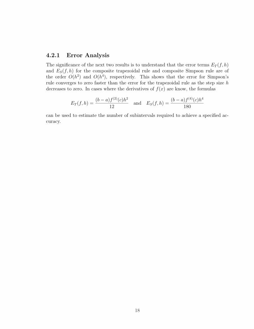
4.2.1 Error Analysis

The significance of the next two results is to understand that the error terms ET (f, h)and ES(f, h) for the composite trapezoidal rule and composite Simpson rule are ofthe order O(h2) and O(h4), respectively. This shows that the error for Simpson’srule converges to zero faster than the error for the trapezoidal rule as the step size hdecreases to zero. In cases where the derivatives of f(x) are know, the formulas

ET (f, h) =(b− a)f (2)(c)h2

12and ES(f, h) =

(b− a)f (4)(c)h4

180

can be used to estimate the number of subintervals required to achieve a specified ac-curacy.

18

98Corollary 2.2 (Trapezoidal Rule: Error Analysis). Suppose that [a, b] is subdi-vided into M subintervals [xk, xk+1] of width h = (b−a)/M . The composite trapezoidalrule

T (f, h) =h

2(f(a) + f(b)) + h

M−1∑

k=1

f(xk) (4.29)

is an approximation to the integral

∫ b

af(x)dx = T (f, h) + ET (f, h). (4.30)

Furthermore, if f ∈ C2[a, b], there exists a value c with a < c < b so that the errorterm ET (f, h) has the form

ET (f, h) =(b− a)f (2)(c)h2

12= O(h2). (4.31)

Proof. We first determine the error term when the rule is applied over [x0, x1]. Inte-grating the Lagrange polynomial P1(x) and its remainder yields

∫ x1

x0

f(x)dx =∫ x1

x0

P1(x)dx +∫ x1

x0

(x− x0)(x− x1)f(2)(c(x))

2!dx. (4.32)

The term (x−x0)(x−x1) does not change sign on [x0, x1], and f (2)(c(x)) is continuous.Hence the second Mean Value Theorem for integrals implies that there exists a valuec1 so that

∫ x1

x0

f(x)dx =h

2(f0 + f1) + f (2)(c1)

∫ x1

x0

(x− x0)(x− x1)

2!dx. (4.33)

Use the change of variable x = x0 + ht in the integral on the right side of (2.33):

∫ x1

x0

f(x)dx =h

2(f0 + f1) +

f (2)(c1)

2

∫ 1

0h(t− 0)h(t− 1)hdt

=h

2(f0 + f1) +

f (2)(c1)h3

2

∫ 1

0(t2 − t)dt (4.34)

=h

2(f0 + f1)− f (2)(c1)h

3

12.

Now we are ready to add up the error terms for all of the intervals [xk, xk+1]:

∫ b

af(x) =

M∑

k=1

∫ xk

xk−1

f(x)dx

19

=M∑

k=1

h

2(f(xk−1) + f(xk))− h3

12

M∑

k=1

f (2)(ck). (4.35)

The first sum is the composite trapezoidal rule T (f, h). In the second term, one factorof h is replaced with its equivalent h = (b− a)/M , and the result is

∫ b

af(x)dx = T (f, h)− (b− a)h2

12

(1

M

M∑

k=1

f (2)(ck)

).

The term in parentheses can be recognized as an average of values for the secondderivative and hence is replaced by f (2)(c). Therefore, we have established that

∫ b

af(x)dx = T (f, h)− (b− a)f (2)(c)h2

12,

and the proof of Corollary 2.2 is complete.

Corollary 2.3 (Simpson’s Rule: Error Analysis). Suppose that [a, b] is subdi-vided into 2M subintervals [xk, xk+1] of equal width h = (b− a)/(2M). The compositeSimpson rule

S(f, h) =h

3(f(a) + f(b)) +

2h

3

M−1∑

k=1

f(x2k) +4h

3

M∑

k=1

f(x2k−1) (4.36)

is an approximation to the integral∫ b

af(x)dx = S(f, h) + ES(f, h). (4.37)

Furthermore, if f ∈ C4[a, b], there exists a value c with a < c < b so that the errorterm ES(f, h) has the form

ES(f, h) =(b− a)f (4)(c)h4

180= O(h4) (4.38)

Example 2.7. Consider f(x) = 2+sin(2√

x). Investigate the error then the compositetrapezoidal rule is used over [1, 6] and the number of subintervals is 10, 20, 40, 80, and160.

Table 2.2. The Composite Trapezoidal Rule forf(x) = 2 + sin(2

√x) over [1, 6]

M h T (f, h) ET (f, h) = O(h2)10 0.5 8.19385457 0.0103754020 0.25 8.18604926 0.0025700640 0.125 8.18412019 0.0006409880 0.0625 8.18363936 0.00016015160 0.03125 8.18351924 0.00004003

20

Table 2.2 shows the approximations T (f, h). The antiderivative of f(x) is

F (x) = 2x−√x cos(2√

x) +sin(2

√x)

2,

and the true value of the definite integral is∫ 6

0f(x)dx = F (x)

∣∣∣x=6

x=1= 8.1834792077.

This value was used to compute the values ET (f, h) = 8.1834792077−T (f, h) in Table2.2. It is important to observe that when h is reduced by a factor of 1

2the successive er-

rors ET (f, h) are diminished by approximately 14. This confirms that the order is O(h2).

Example 2.8. Consider f(x) = 2+sin(2√

x). Investigate the error when the compos-ite Simpson rule is used over [1, 6] and the number of subintervals is 10, 20, 40, 80,and160.

Table 2.3 shows the approximations S(f, h). The true value of the integral is8.1834792077, which was used to compute the values ES(f, h) = 8.1834792077−S(f, h)in Table 2.3. It is important to observe that when h is reduced by a factor of 1

2the

successive errors ES(f, h) are diminished by approximately 116

. This confirms that theorder is O(h4).

Table 2.3 The Composite Simpson Rule forf(x) = 2 + sin(2

√x) over [1, 6]

M h S(f, h) ES(f, h) = O(h4)5 0.5 8.18301549 0.0004637110 0.25 8.18344750 0.0000317120 0.125 8.18347717 0.0000020440 0.0625 8.18347908 0.0000001380 0.03125 8.18347920 0.00000001

Example 2.9. Find the number M and the step size h so that the error ET (f, h) for thecomposite trapezoidal rule is less than 5×10−9 for the approximation

∫ 72 dx/x ≈ T (f, h).

The integrand is f(x) = 1/x and its first two derivatives are f ′(x) = −1/x2 andf ′′(x) = 2/x3. The maximum value of |f ′′(x)| taken over [2, 7] occurs at the end point,x = 2 and thus we have the bound |f ′′(c)| ≤ |f ′′(2)| = 1

4, for 2 ≤ c ≤ 7. This is used

with formula (2.31) to obtain

|ET (f, h)| = | − (b− a)f ′′(c)h2|12

≤ (7− 2)14h2

12=

5h2

48. (4.39)

The step size h and number M satisfy the relation h = 5/M , and this is used in (2.39)to get the relation

|ET (f, h)| ≤ 125

48M2≤ 5× 10−9. (4.40)

21

Now rewrite (2.40) so that it is easier to solve for M:

25

48× 109 ≤ M2 (4.41)

Solving (2.41), we find that 22821.77 ≤ M . Since M must be an integer, we chooseM = 22, 822 and the corresponding step size is h = 5/22, 822 = 0.000219086846. Whenthe composite trapezoidal rule is implemented with this many function evaluations,there is a possibility that the rounded-off function evaluations will produce a significantamount of error. When the computation was performed, the result was

T (f,5

22, 822) = 1.252762969,

which compares favorably with the true value∫ 72 dx/x = ln(x)|x=7

x=2 = 1.252762968. Theerror is smaller than predicted because the bound 1

4for |f ′′(c)| was used. Experimen-

tation shows that it takes about 10,001 function evaluations to achieve the desiredaccuracy of 5 × 10−9, and when the calculation is performed with M = 10, 000, theresult is

T (f,5

10, 000) = 1.252762973.

The composite trapezoidal rule usually requires a large number of function eval-uations to achieve an accurate answer. This is contrasted in the next example withSimpson’s rule, which will require significantly fewer evaluations.

Example 2.10. Find the number M and the step size h so that the error ES(f, h)for the composite Simpson rule is less than 5× 10−9 for the approximation

∫ 72 dx/x ≈

S(f, h).The integrand is f(x) = 1/x, and f (4)(x) = 24/x5. The maximum value of |f (4)(c)|

taken over [2, 7] occurs at the end point x = 2, and thus we have the bound |f (4)(c)| ≤|f (4)(2)| = 3

4for 2 ≤ c ≤ 7. This is used with formula (2.38) to obtain

|ES(f, h) =| − (b− a)f (4)(c)h4|

180≤ (7− 2)3

4h4

180=

h4

48. (4.42)

The step size h and number M satisfy the relation h = 5/(2M), and this is used in(2.42) to get the relation

|ES(f, h)| ≤ 625

768M4≤ 5× 10−9. (4.43)

Now rewrite (2.43) so that it is easier to solve for M :

125

768× 10−9 ≤ M4. (4.44)

22

Solving (2.44), we find that 112.95 ≤ M , Since M must be an integer, we choseM = 113, and the corresponding step size is h = 5/226 = 0.02212389381. When thecomposite Simpson rule was performed, the result was

S(f,5

226) = 1.252762969,

which agrees with∫ 72 dx/x = ln(x)|x=7

x=2 = 1.252762968. Experimentation shows that ittakes about 129 function evaluations to achieve the desired accuracy of 5 × 10−9, andwhen the calculation is performed with M = 64, the result is

S(f,5

128) = 1.252762973.

So we see that the composite Simpson rule using 229 evaluations of and the com-posite trapezoidal rule using 22,823 evaluations of f(x) achieve the same accuracy. InExample 2,10, Simpson’s rule required about 1/100 the number of function evaluations.

Program 2.1 (Composite Trapezoidal Rule). To approximate the integral∫ ba f(x)dx = h

2(f(a) + f(b)) + h

M−1∑k=1

f(xk)

by sample f(x) at the M + 1 equally spaced points xk = a + kh, for k = 0, 1, 2,. . . , M . Notice that x0 = a and xM = b.

Function s=traprl(f,a,b,M)%Input - f is the integrand input as a string ’f’% - a and b are upper and lower limits of integration% - M is the number of subintervals%Output - s is the trapezoidal rule sumh=(b-a)/M;s=0;for k=1:(M-1)

x=a+h*k;s=s+feval(f,x);

ends=h*(feval(f,a)+feval(f,b)/2+h*s;

Program 7.2 (Composite Simpson Rule). To approximate the integral∫ ba f(x)dx = h

3(f(a) + f(b)) + 2h

3

M−1∑k=1

f(x2k) + 4h3

M∑k=1

f(x2k−1)

by sample f(x) at the 2M + 1 equally spaced points xk = a + kh, for k = 0, 1, 2,. . . , 2M . Notice that x0 = a and x2M = b.

23

Function s=simprl(f,a,b,M)%Input - f is the integrand input as a string ’f’% - a and b are upper and lower limits of integration% - M is the number of subintervals%Output - s is the simpson rule sumh=(b-a)/(2*M);s1=0s2=0;for k=1:M

x=a+h*(2k-1);s1=s1+feval(f,x);

endfor k=1:(M-1)

x=a+h+2*k;s2=s2+feval(f,x);

ends=h*(feval(f,a)+feval(f,b)+4*s1+2*s2)/3;

4.3 Exercises For Composite Trapezoidal and Simp-

son’s Rule

1. (i) Approximate each integral using the composite trapezoidal rule withM = 10.

(ii) Approximate each integral using the composite Simpson rule withM = 5.

(a)∫ 1−1(1 + x2)−1dx (b)

∫ 10 (2 + sin(2

√x)dx (c)

∫ 40.25 dx/

√x

(d)∫ 40 x2e−xdx (e)

∫ 20 2x cos(x)dx (f)

∫ π0 sin(2x)e−xdx

2. Length of a curve. The arc length of the curve y = f(x) over the intervala ≤ x ≤ b is

length =∫ b

a

√1 + (f ′(x)2)dx

(i) Approximate the arc length of each function using the composite trape-zoidal rule with M = 10.

(ii) Approximate the arc length of each function using the composite Simp-son rule with M = 5.

(ii) Approximate the surface area using the composite Simpson rule withM = 5.

(a) f(x) = x3 for 0 ≤ x ≤ 1(b) f(x) = sin(x) for 0 ≤ x ≤ π/4

24

(c) f(x) = e−x for 0 ≤ x ≤ 14. (a) Verify that the trapezoidal rule (M = 1, h = 1) is exact for polynomials

of degree ≤ of the form f(x) = c1x + c0 over [0, 1].(b) Use the integrand f(x) = c2x

2 and verify that the error term for thetrapezoidal rule M = 1, h = 1) over the interval [0, 1] is

ET (f, h) =(b− a)f (2)h2

12.

5. (a) Verify that Simpson’s rule (M = 1, h = 1) is exact for polynomials ofdegree ≤ 3 of form f(x) = c3x

3 + c2x2 + c1x + c0 over [0, 2].

(b) Use the integrand f(x) = c4x4 and verify that the error term for

Simpson’s rule (M = 1, h = 1) over the interval [0, 2] is

ES(f, h) =(b− a)f (4)(c)h4

180

6. Derive the trapezoidal rule M = 1, h = 1) by using the method of undeter-mined coefficients.(a) Find the constants w0 and w1 so that

∫ 10 g(t)dt = w0g(0) + w1g(1) is

exact for the two functions g(t) = 1 and g(t) = t.(b) Use the relation f(x0 + ht) = g(t) and the change of variable x = x0 + ht

and dx = hdt to translate the trapezoidal rule over [0, 1] to the interval [x0, x1].Hint for part (a). You will get a linear system involving the two unknowns w0, and

w1.7. Derive Simpson’s rule (M = 1, h = 1) by using the method of undeterminedcoefficients.

(a) Find the constants w0, w1, and w2 so that∫ 20 g(t)dt = w0g(0)+w1g(1)+w2g(2)

is exact for the three functions g(t) = 1, g(t) = t, and g(t) = t2.(b) Use the relation f(x0 + ht) = g(t) and the change of variable x = x0 + ht and

dx = hdt to translate the trapezoidal rule over [0, 2] to the interval [x0, x2].Hint for part (a) You will get a linear system involving the three unknowns w0, w1,

and w2.8. Determine the number M and the interval width h so that the composite trapezoidalrule for M subintervals can be used to compute the given integral with an accuracy of5× 10−9.

(a)∫ π/6

−π/6cos(x)dx (b)

∫ 3

2

1

5− xdx (c)

∫ 2

0xe−xdx

Hint for part (c) f (2)(x) = (x− 2)e−x.9. Determine the number M and the interval width h so that the composite Simpsonrule for 2M subintervals can be used to compute the given integral with an accuracy

25

of 5× 10−9.

(a)∫ π/6

−π/6cos(x)dx (b)

∫ 3

2

1

5− xdx (c)

∫ 2

0xe−xdx

Hint for part (c) f (4)(x) = (x− 4)e−x.CHQP .7NUMERICAL INTEGRATION 10.consider the definite integral .The fol-

lowing table gives approximations using the composite trapezoidal rule .Calculate andconfirm that the order is 11.Consider the definite integral .The following table givesapproximations using the composite Simpson rule .Calculate and confirm that the or-der is 12.Midpoint rule .The midpoint rule on is (a) Expand ,the ant antiderivativeof, in a Taylor series about and establish the midpoint rule on (b) Use part (a) andshoe that the composite midpoint rule for approximating the integral of is This isan approximation to the integral of over and we write (c) Show that the error termfor part is 13.Use the midpoint rule with to approximate the integrals in Exercise 1.14.Prove Corollary 7.3. SEC.7.2 COMPOSITE TRAPEZOIDAL AND SIMPSON’SRULE Algorithms and Programs 1.(a) For each integral in Exercise 1,compute Mandthe interval width h so that the composite trapezoidal rule can be used to compute thegiven integral with an accuracy of nine decimal places .Use Program 7.1 to approximateeach integral. (b )For each integral in Exercise 1, compute M and the interval width hso that the composite Simpson’s rule can be used to compute the given integral with anaccuracy of nine4 decimal places .Use Program 7.2 to approximate each integral 2.UseProgram 7.2 to approximate the definite integrals in Exercise 2 with an accuracy of 11decimal places. 3.The composite trapezoidal rule can adapted to integrate a functionknown only at a set of points .Adapt Program 7.1 to approximate the integral of afunction over an interval that passes through M given points (Note. The nodes neednot be equally spaced .)Use this program to approximate the integral of a function thatpasses through the points 5.Modify Program 7.1 so that it uses the composite midpointrule (Exercise 12)to approximate the integral of .Use this program to approximate thedefinite integrals in Exercise 1 with an accuracy of 11decimal places. 6.Obtain approx-imations to each of the following definite integrals with an accuracy of ten decimalplaces.Use any of the programs from this section 7.The following example shows howSimpson’s rule can be used to approximate the solution of an integral equation .Theequation be solved using Simpson’s rule with; then let Substituting into equation (1)yields the system of Linear equations: Subsuming the solution of system into equa-tion and simplifying yields the approximation (a) As a check, substitute the solutionright-hand side of the integral equation, integrate and simplify the right-hand side, andcompare the result with the approximation in (3) (b) Use the composite Simpson rulewith to approximate the solution of the integral equation Use the procedure outlinedin part (a )to check your solution.

26

4.4 Recursive Rules and Romberg Integration

In this section we show how to compute Simpson approximations with a special linearcombination of trapezoidal rules. The approximation will have greater accuracy if oneuses a larger number of subintervals. How many should we choose? The sequentialprocess helps answer this question by trying two subintervals, four subintervals, andso on, until the desired accuracy is obtained. First, a sequence {T (J)} of trapezoidalrule approximations must be generated. As the number of subintervals is doubled, thenumber of function values is roughly doubled, because the function must be evaluatedat all the previous points and at the midpoints of the previous subintervals (see Fig-ure 2.8). Theorem 2.4 explains how to eliminate redundant function evaluations andadditions.

Theorem 7.4 (Successive Trapezoidal Rules). Suppose that J ≥ 1 and the points{xk = a+kh} subdivide [a, b] into 2J = 2M subintervals of equal width h = (b−a)/2J .The trapezoidal rules T (f, h) and T (f, 2h) obey the relationship

T (f, h) =T (f, 2h)

2+ h

M∑

k=1

f(x2k−1). (4.45)

Definition 2.3 (Sequence of Trapezoidal Rules). Define T (0) = (h/2)(f(a) +f(b)), which is the trapezoidal rule with step size h = b. Then for each J ≥ 1 defineT (J) = T (f, h), where T (f, h) is the trapezoidal rule with step size h = (b− a)/2J .

Corollary 7.4 (Recursive Trapezoidal Rule). Start with T (0) = (h/2)(f(a) +f(b)). Then a sequence of trapezoidal rules {T (J)} is generated by the recursive for-mula

T (J) =T (J − 1)

2+ h

M∑

k=1

f(x2k−1) for J = 1, 2, . . . , (4.46)

where h = (b− a)/2J and {xk = a + kh}.Proof. For the even nodes x0 < x2 < · · · < x2M−2 < x2M , we use the trapezoidal rulewith step size 2h:

T (J − 1) =2h

2(f0 + 2f2 + 2f4 + · · ·+ 2f2M−4 + 2f2M−2 + f2M). (4.47)

For all of the nodes x0 < x1 < x2 < · · · < x2M−1 < x2M , we use the trapezoidal rulewith step size h:

T (J) =h

2(f0 + 2f1 + 2f2 + · · ·+ 2f2M−2 + 2f2M−1 + f2M). (4.48)

Collecting the even and odd subscripts in (2.48) yields

T (J) =h

2(f0 + 2f2 + · · ·+ 2f2M−2 + f2M) + h

M∑

k=1

f2k−1. (4.49)

27

Substituting (2.47) into (2.49) results in T (J) = T (J − 1)/2 + h∑M

k=1 f2k−1, and theproof of the theorem is complete.

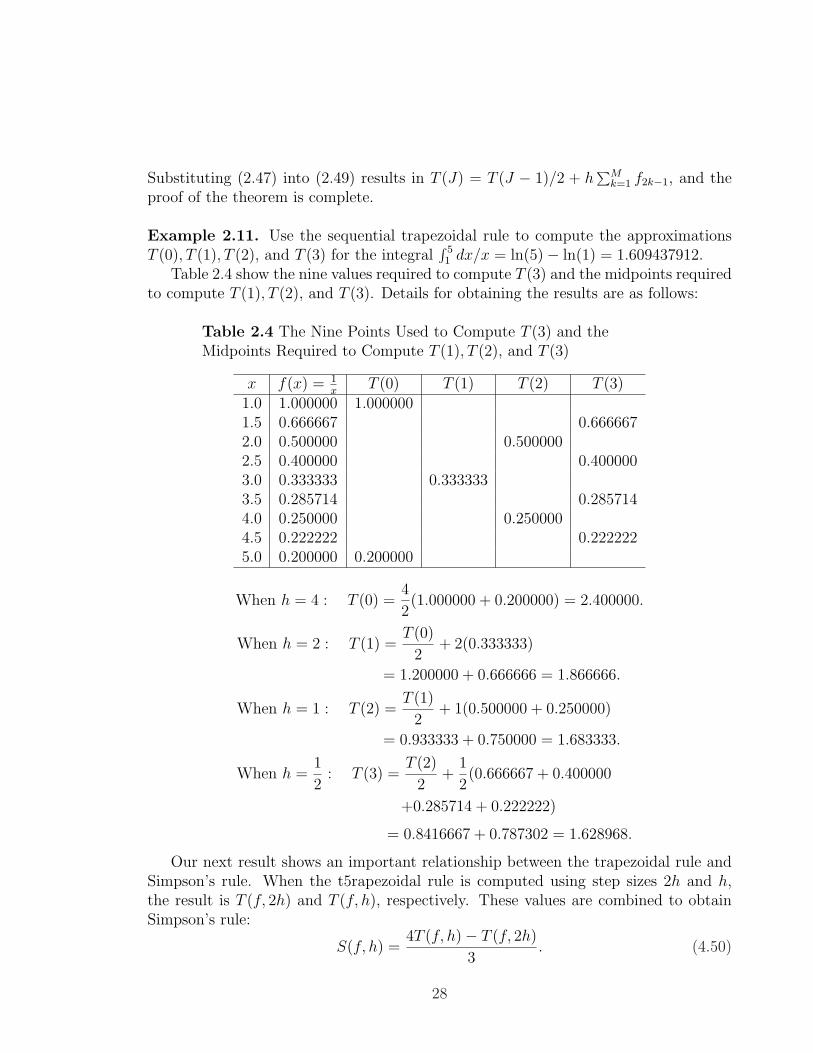
Example 2.11. Use the sequential trapezoidal rule to compute the approximationsT (0), T (1), T (2), and T (3) for the integral

∫ 51 dx/x = ln(5)− ln(1) = 1.609437912.

Table 2.4 show the nine values required to compute T (3) and the midpoints requiredto compute T (1), T (2), and T (3). Details for obtaining the results are as follows:

Table 2.4 The Nine Points Used to Compute T (3) and theMidpoints Required to Compute T (1), T (2), and T (3)

x f(x) = 1x

T (0) T (1) T (2) T (3)1.0 1.000000 1.0000001.5 0.666667 0.6666672.0 0.500000 0.5000002.5 0.400000 0.4000003.0 0.333333 0.3333333.5 0.285714 0.2857144.0 0.250000 0.2500004.5 0.222222 0.2222225.0 0.200000 0.200000

When h = 4 : T (0) =4

2(1.000000 + 0.200000) = 2.400000.

When h = 2 : T (1) =T (0)

2+ 2(0.333333)

= 1.200000 + 0.666666 = 1.866666.

When h = 1 : T (2) =T (1)

2+ 1(0.500000 + 0.250000)

= 0.933333 + 0.750000 = 1.683333.

When h =1

2: T (3) =

T (2)

2+

1

2(0.666667 + 0.400000

+0.285714 + 0.222222)

= 0.8416667 + 0.787302 = 1.628968.

Our next result shows an important relationship between the trapezoidal rule andSimpson’s rule. When the t5rapezoidal rule is computed using step sizes 2h and h,the result is T (f, 2h) and T (f, h), respectively. These values are combined to obtainSimpson’s rule:

S(f, h) =4T (f, h)− T (f, 2h)

3. (4.50)

28

Theorem 2.5 (Recursive Simpson Rules). Suppose that {T (J)} is the sequenceof trapezoidal rules generated by Corollary 2.4. If J ≥ 1 and S(J) is Simpson’s rule for2J subintervals of [a, b], then S(J) and the trapezoidal rules T (J − 1) and T (J) obeythe relationship

S(J) =4T (J)− T (J − 1)

3for J = 1, 2, . . . . (4.51)

Proof. The trapezoidal rule T (J) with step size h yields the approximation

∫ b

af(x)dx ≈ h

2(f0 + 2f1 + 2f2 + · · ·+ 2f2M−2 + 2f2M−1 + f2M) = T (J). (4.52)

The trapezoidal rule T (J − 1) with step size 2h produces

∫ b

af(x)dx ≈ h(f0 + 2f2 + · · ·+ 2f2M−2 + f2M) = T (J − 1). (4.53)

Multiplying relation (2.52) by 4 yields

4∫ b

af(x)dx ≈ h(2f0 + 4f1 + 4f2 + · · ·+ 4f2M−2 + 4f2M−1 + 2f2M) = 4T (J). (4.54)

Now subtract(2.53)from (2.54)and the result is

3∫ b

af(x)dx ≈ h(f0+4f1+2f2+· · ·+2f2M−2+4f2M−1+f2M) = 4T (J)−T (J−1). (4.55)

This can be rearranged to obtain

∫ b

af(x)dx ≈ h

3(f0 + 4f1 + 2f2 + · · ·+ 2f2M−2 + 4f2M−1 + f2M) =

4T (J)− T (J − 1)

3.

(4.56)The middle term in (2.57) is Simpson’s rule S(J) = S(f, h) and hence the theorem isproved.

Example 2.12. Use the sequential Simpson rule to compute the approximationsS(1), S(2), and S(3) for the integral of Example 2.11.

Using the results of Example 2.11 and formula (2.50) with J = 1, 2, and 3, wecomputes

S(1) =4T (1)− T (0)

3=

4(1.866666)− 2.400000

3= 1.688888.

S(2) =4T (2)− T (1)

3=

4(1.683333)− 1.8666666

3= 1.622222

29

S(3) =4T (3)− T (2)

3=

4(1.628968)− 1.683333

3= 1.610846.

In Section 2.1 the formula for Boole’s rule was given in Theorem 2.1. It was obtainedby integrating the Lagrange polynomial of degree 4 based on the nodes x0, x1, x2, x3, andx4. An alternative method for establishing Boole’s rule is mentioned in the exercises.When it is applied M times over 4M equally spaced subintervals of [a, b] of step sizeh = (b− a)/(4M), we call it the composite Boole rule:

B(f, h) =2h

45

M∑

k=1

(7f4k−4 + 32f4k−3 + 12f4k−2 + 32f4k−1 + 7f4k). (4.57)

The next result gives the relationship between the sequential Boole and Simpson rules.

Theorem 2.6 (Recursive Boole Rules). Suppose that {S(J)} is the sequenceof Simpson’s rules generated by Theorem 2.5. If J ≥ 2 and B(J) is Boole’s rule for2J subintervals of [a, b], then B(J) and Simpson’s rules S(J − 1) and S(J) obey therelationship

B(J) =16S(J)− S(J − 1)

15for J = 2, 3, . . . . (4.58)

Proof. The proof is left as an exercise for reader.

Example 2.13. Use the sequential Boole rule to compute the approximations B(2)and B(3) for the integral of Example 2.11.

Using the results of Example 2.12 and formula (2.59) with J = 2 and 3, we compute

B(2) =16S(2)− S(1)

15+

16(1.622222)− 1.688888

15= 1.617778.

B(3) =16S(3)− S(2)

15=

16(1.610846)− 1.622222

15= 1.610088.

The reader may wonder what we are leading up to. We will now show that for-mulas (2.50)and (2.59) are special cases of the process of Romberg integration. Let usannounce that the next level of approximation for the integral of Example 2.11 is

64B(3)−B(2)

63=

64(1.610088)− 1.617778

63= 1.609490,

and this answer gives an accuracy of five decimal places.

4.5 Romberg Integration

In Section 2.2 we saw that the error terms ET (f, h) and ES(f, h) for the compositetrapezoidal rule and composite Simpson rule are of order O(h2) and O(h4), respectively.

30

It is not difficult to show that the error term EB(f, h) for the composite Boole rule isof the order O(h6). Thus we have the pattern

∫ b

af(x)dx = T (f, h) + O(h2). (4.59)

∫ b

af(x)dx = S(f, h) + O(h4). (4.60)

∫ b

af(x)dx = B(f, h) + O(h6). (4.61)

The pattern for the remainders in (2.60) through (2.62) is extended in the fol-lowing sense. Suppose that an approximation rule is used with step sizes h and 2h;then an algebraic manipulation of the two answers is used to produce an improved an-swer. Each successive level of improvement increases the order of the error term fromO(h2N) to O(h2N+2). This process, called Romberg integration , has its strengthsand weaknesses.

The Newton-Cotes rules are seldom used past Boole’s rule. This is because the nine-point Newton-Cotes quadrature rule involves negative weights, and all the rules pastthe ten-point rule involve negative weights. This could introduce loss of significanceerror due to round off. The Romberg method has the advantages that all the weightsare positive and the equally spaced abscissas are easy to compute.

A computational weakness of Romberg integration is that twice as many functionevaluations are needed to decrease the error from O(h2N) to O(h2N+2). The use of thesequential rules will help keep the number of computations down. The development ofRomberg integration relies on the theoretical assumption that, if f ∈ CN [a, b] for allN , then the error term for the trapezoidal rule can be represented a series involvingonly even powers of h; that is,

∫ b

af(x)dx = T (f, h) + ET (f, h), (4.62)

whereET (f, h) = a1h

2 + a2h4 + a3h

6 + · · · , (4.63)

A derivation of formula (2.64) can be found in Reference [153].Since only even powers of h can occur in (1.64), the Richardson improvement process

is used successively first to eliminate a1, next to eliminate a2, then to eliminate a3. andso on. This process generates quadrature formulas whose error terms have even ordersO(h4), O(h6), O(h8), and so on. We shall show that the first improvement is Simpson’srule for 2M intervals. Start with T (f, 2h) and T (f, h) and the equations

∫ b

af(x)dx = T (f, 2h) + a14h

2 + a216h4 + a364h6 + · · · (4.64)

31

and ∫ b

af(x)dx = T (f, h) + a1h

2 + a2h4 + a3h

6 + · · · (4.65)

Multiply equation (2.66) by 4 and obtain

4∫ b

af(x)dx = 4T (f, h) + a14h

2 + a24h4 + a34h

6 + · · · . (4.66)

Eliminate a1 by subtracting (2.65) from (2.67). The result is

3∫ b

af(x)dx = 4T (f, h)− T (f, 2h)− a212h4 − a360h6 + · · · . (4.67)

Now divide equation (2.68) by 3 and rename the coefficients in the series:

∫ b

af(x)dx =

4T (f, h)− T (f, 2h)

3+ b1h

4 + b2h6 + · · · . (4.68)

As noted in (2.49), the first quantity on the right side of (2.69) is Simpson’s rule S(f, h).This shows that ES(f, h) involves only even powers of h:

∫ b

af(x)dx = S(f, h) + b1h

4 + b2h6 + b3h

8 + · · · . (4.69)

To show that the second improvement is Boole’s rule, start with (2.70) and writedown the formula involving S(f, 2h):

∫ b

af(x)dx = S(f, 2h) + b116h4 + b264h6 + b3256h8 + · · · . (4.70)

When b1 is eliminated from (2.70) and (2.71), the result involves Boole’s rule:

∫ b

af(x)dx =

16S(f, h)− S(f, 2h)

15− b248h6

15− b3240h8

15· · · (4.71)

= B(f, h)− b248h6

15− b3240h8

15· · · .

The general pattern for romberg integration relies on lemma 2.1.

Lemma 2.1 (Richardson’s Improvement for Romberg integration). Giventwo approximations R(2h,K − 1) and R(h,K − 1) for the quantity Q that satisfy

Q = R(h,K − 1) + c1h2K + c2h

2K+2 + · · · (4.72)

andQ = R(2h,K − 1) + c14

Kh2K + c24K+1h2K+2 + · · · , (4.73)

32

an improved approximation has the form

Q =4KR(h,K − 1)−R(2h,K − 1)

4K − 1+ O(h2K+2). (4.74)

The proof is straightforward and is left for the reader.

Definition 2.4. Define the sequence {R(J,K) : J ≥ K}∞J=0 of quadrature formu-las for f(x) over [a, b] as follows

R(J, 0) = T (J) for J ≥ 0, is the sequential trapezoidal rule.R(J, 1) = S(J) for J ≥ 1, is the sequential Simpson rule.R(J, 2) = B(J) for J ≥ 2, is the sequential Boole’s rule.

(4.75)

The starting rules, {R(J, 0)}, are used to generate the first improvement, {R(J, 1)},which in turn is used to generate the second improvement, {R(J, 2)}. We have alreadyseen the patterns

R(J, 1) =41R(J, 0)−R(J − 1, 0)

41 − 1for J ≥ 1 (4.76)

R(J, 2) =42R(J, 1)−R(J − 1, 1)

42 − 1for J ≥ 2,

which are rules in (2.69) and (2.72) stated using the notation in (2.71). The generalrule for constructing improvements is

R(J,K) =4KR(J,K − 1)−R(J − 1, K − 1)

4K − 1for J ≥ K. (4.77)

Table 2.5 Romberg Integration Tableau

J R(J,0) R(J,1) R(J,2) R(J,3) R(J,4)0 R(0,0)1

Table 7.6 Romberg Integration Tableau for example 7.14For computational purposes, the values are arranged in the romberg integration

tableau given in table 7.5. Example 7.14. Use Romberg integration to find approxima-tions for the definite integral The computations are given in table 7.6. In each columnthe numbers are converging to the value 2.038197427067 the values in the simpson’srule column converge faster than the values in the trapezoidal rule column. For thisexample, convergence in columns to the right is faster than the adjacent column to theleft. Convergence of the Romberg values in table 7.6 is easier to see if we lood at theerror terms . suppose that the interval width is a and that the higher derivatives of

33

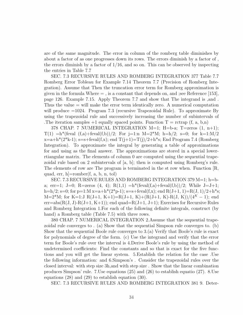
are of the same magnitude. The error in column of the romberg table diminishes byabout a factor of as one progresses down its rows. The errors diminish by a factor of ,the errors diminish by a factor of 1/16, and so on. This can be observed by inspectingthe entries in Table 7.7

SEC. 7.3 RECURSIVE RULES AND ROMBERG INTEGRATION 377 Table 7.7Romberg Error Tobleau for Example 7.14 Theorem 7.7 (Precision of Romberg Inte-gration). Assume that Then the truncation error term for Romberg approximation isgiven in the formula Where = , is a constant that depends on, and ;see Reference [153],page 126. Example 7.15. Apply Theorem 7.7 and show that The integrand is ,and .Thus the value = will make the error term identically zero. A numerical computationwill produce =1024. Program 7.3 (recursive Trapezoidal Rule). To approximate Byusing the trapezoidal rule and successively increasing the number of subintervals of.The iteration samples +1 equally spaced points. Function T = rctrap (f, a, b,n)

378 CHAP. 7 NUMERICAL INTEGRATION M=1; H=b-a; T=zeros (1, n+1);T(1) =h*(feval (f,a)+feval(f,b))/2; For j=1:n M=2*M; h=h/2; s=0; for k=1:M/2x=a+h*(2*k-1); s=s+feval(f,x); end T(j+1)=T(j)/2+h*s; End Program 7.4 (RombergIntegration). To approximate the integral by generating a table of approximationsfor and using as the final answer. The approximations are stored in a special lower-rtiangular matrix. The elements of column 0 are computed using the sequential trape-zoidal rule based on 2 subintervals of [a, b]; then is computed using Romberg’s rule.The elements of row are The program is terminated in the st row when. Function [R,quad, err, h]=romber(f, a, b, n, tol)

SEC. 7.3 RECURSIVE RULES AND ROMBERG INTEGRATION 379 M=1; h=b-a; err=1; J=0; R=zeros (4, 4); R(1,1) =h*(feval(f,a)+feval(f,b))/2; While J=J+1;h=h/2; s=0; for p=1:M x=a+h*(2*p-1); s=s+feval(f,x); end R(J+1, 1)=R(J, 1)/2+h*s;M=2*M; for K=1:J R(J+1, K+1)=R(J+1, K)+(R(J+1, K)-R(J, K))/(4K − 1); enderr=abs(R(J, J)-R(J+1, K+1)); end quad=R(J+1, J+1); Exercises for Recursive Rulesand Romberg Integration 1.For each of the following definite integrals, construct (byhand) a Romberg table (Table 7.5) with three rows.

380 CHAP. 7 NUMERICAL INTEGRATION 2.Assume that the sequential trape-zoidal rule converges to . (a) Show that the sequential Simpson rule converges to. (b)Show that the sequential Boole rule converges to 3.(a) Verify that Boole’s rule is exactfor polynomials of degree of the form. (c) Use the integrand and verify that the errorterm for Boole’s rule over the interval is 4.Derive Boole’s rule by using the method ofundetermined coefficients: Find the constants and so that is exact for the five func-tions and you will get the linear system. 5.Establish the relation for the case .Usethe following information: and 6.Simpson’s . Consider the trapezoidal rules over theclosed interval: with step size 3h,and with step size . Show that the linear combinationproduces Simpson’ rule. 7.Use equations (25) and (26) to establish equatio (27). 8.Useequations (28) and (29) to establish equation (30).

SEC. 7.3 RECURSIVE RULES AND ROMBERG INTEGRATION 381 9. Deter-

34

mine the smallest integer K for which 10.Romberg integration was used to approximatethe integrals , and the results are given in the following table: (a) Use the change ofvariable and and show that the two integrals have the same numerical (ii). 11.Rombergintegration based on the midpoint rule. The composite midpoint rule is competitivewith the composite trapezoidal rule with respet to efficiency and the speed of con-vergence. Use the following facts about the midpoint rule: The rule and the errorterm are given by and (a) Start with Develop the sequential midpoint rule for comput-ing (b) Show how the sequential midpoint rule can be used in place of the sequentialtrapezoidal rule in Romberg integration. 382 CHAP. 7 NUMERICAL INTEGRATIONAlgorithms and Programs 1.Use Program 7.4 to approximate the definite integrals inExercise l with an accuracy of ll decimal places. 2.Use Program 7.4 to approximate thefollowing two definite integrals with an accuracy of 10 decimal places. The exact valueof each definite integral is . Explain any apparent differences in the rates of convergenceof the two Romberg sequences. 3.The normal probability density funcion is , and thecumulative distribution is a function defined by the integral Compute values for , andthat have eight digits of accuracy. 4.Modiry Program 7.3 so that it will also computevalues for the sequential Simpson and Boole rules. 5.Modify Program 7.3 so that it willalso compute values for the sequential Simpson and Boole rules. 6.Modify Program 7.4so that it uses the sequential midpoint rule to perform Romberg integration (use theresults of Exercise ll). Use your program to approximate the following integrals with anaccuracy of 10 decimal places. 7.In Program 7.4 the approximations to a given definiteintegral are stored on the main diagonal of a lower-triangular matrix. Modify Program7.4 so that the rows of the Romberg integration tableau are sequentially computedand stored in matrix R; hence it saves space. Test your program on the integrals inExercise l. Adaptive Quadrature The composite quadrature rules necessitate the useof equally spaced points. Typically, a small step size h was used uniformly acroff theentire interval of integration to ensure the overall accuracy. This does not take into ac-count that some portions of the curve may have large functional variations that requiremore attention than other portions of the curve.it is useful to introduce a method thatadjusts the step size to be smaller over portions of the curve where a larger functionalvariation occurs. This technique is called adaptive quadrature. The method is basedon simpson’ s rule. Simpson’s rule uses two subintervals over:

SEC. 7.4 ADAPTIVE QUADRATURE 383 where is the center of = furthermore,if so that Refinement A composite Simpson rule using four subintervals of can be per-formed by bisecting this interval into two equal subintervals and and applying formula(1) recursively over each piece. Only two additional evaluations of are needed, and theresult is wherh is the midpoint of ,and is the midpoint . in formula (3) the step size ish/2, which accounts for the factors h/6 on the right side of the equation. Furthermore,if, there exists a value so that Assume that ; then the right sides of equations (2) and(4) are used to obtain the relation Which can be written as Then (6) is substituted in(4) to obtain the error estimate: Because of the assumption , the fraction is replaced

35

with on the right side of (7) when implementing the method. This justifies the followingtest.

384 CHAP. 7 NUMERICAL INTEGRATION Accuracy Test Assume that the tol-erance is specified for the interval. If we infer that thus the composite simpson rule (3)is used to approximate the integral and the error bound for this approximation overis. Adaptive quadrature is implemented by applying simpson’s rules (1) and (3). Startwith, where is the tolerance for numerical quadrature over. The interval is refined intosubintervals labeled and . if the accuracy test (8) is passed, quadrature formula (3) isapplied to and we are done. If the test in (8) fails, the two subintervals are relabeledand , over which we use the tolerances and , respectively. Thus we have two intervalswith their associated tolerances to consider for further refinement and testing: and ,where ,if adaptive quadrature must be continued, the smaller intervals nust be refinedand tested, each with its own associated tolerance. In the second step we first considerand refine the interval into and . if they pass the accuracy test (8) with the tolerance,quadrature formula (3) is applied to and accuracy has been achieved over this interval.If they fail the test in (8) with the tolerance, each subinterval and must be refined andtested in the third step with the reduced tolerance Moreover, the second step involveslooking at and refining into and . if they pass the accuracy test (8) with tolerance, quadrature formula (3) is applied to and accuracy is achieved over this interval. Ifthey fail the test in (8) with the tolerance, each subinterval and must be refined andtested in the third step with the reduced tolerancee. Therefore, the second step pro-duces either three or four intervals, which we relabel consecutively. The three intervalswould be relabeled to produce. Where . in the case of four intervals, we would obtain ,where. If adaptive quadrature must be continued, the smaller intervals must be tested,each with its own associated tolerance. The error term in (4) shows that each time arefinement is made over a smaller subinterval there is a reduction of error by about

SEC. 7.4 ADAPTIVE QUADRATURE 385 Table 7.8 Adaptive Quadrature Com-putations for A factor of . Thus the process will terminate after a finite number ofsteps. The booddeeping for implementing the metheod includes a sentinel variablewhich indicates if a particular subinterval has passed its accuracy test. To avoid un-necessary additional evaluations of, the function values can be included in a data listcorresponding to each subinterval. The details are shown in program 7.6. Example7.16. Use adaptive quadrature to numerically approximate the value of the definiteintegral with the starting tolerance =0.00001. Implementation of the method revealedthat 20 subintervals are needed. Table 7.8 lists each interval, composite simpson rule ,the error bound for this approximation, and the associated tolerance . the approximatevalue of the integral is obtained by summing the simpson rule approximations to get

386 CHAP. 7 NUMERICAL INTEGRATION The true value of the integral isTherefore, the error for adaptive quadrature is Which is smaller than the specifiedtolerance =0.00001. the adaptive methoe involves 20 subintervals of [0.4]. and 81function evaluations were used. Figure 7.9 shows the graph of and these 20 subintervals.

36

The intervals are smaller where a larger functional variation occurs mear the origin. Inthe refinement and testing process in the adaptive method, the first four intervals werebisected into eight subintervals of width 0.03125. if this uniform spacing is continuedthroughout the interval [0.4], M = 128 subintervals are required for the compositesimpson rule, which yields the approximation 1.54878844029, which is in error by theamount 0.00000006776. although the composite simpson method contains half theerror of the adaptive quadrature method, 176 more function evaluations are required.This gain of accuracy is negligible; hence there is a considerable saving of computingeffort with the adaptive method. Program 7.5, srule, is a modification of simpson’srule from section 7.1. the output is a vector Z that contains the results of simpson’srule on the interval . program 7.6 calls srule as a subroutine to carry out simpson’srule on each of the subintervals generated by the adaptive quadrature process.

SEC. 7.4 ADAPTIVE QUADRATURE 387 Program 7.5 (sipson’s rule). To approx-imate the integral By using simpson’s rule, where Function Z = srule (f, a0, b0, to10)h= C=zeros (1,3); C=feval S= S2=S; Toll=to10; Err=to10; Z=[a0 b0 S S2 err toll];Program 7.6 produces a matrix srmat, quad (adaptive quadrature approximation todefinite integral) and err (the error bound for the approximation). The rows of srmatconsist of the end points, the simpson’s rule approximation,and the error bound oneach subinterval generated by the adaptive quadrature process. Program 7.6 (adaptivequadrature using simpson’s rule). To approximate the integral The composite simpsonrule is applied to the 4M subintervals, where and function [srmat, quad, err] =adapt(f, a, b, tol)

388 CHAP. 7 NUMERICAL INTEGRATION srmat = zeros (30,6); iterating =0; done = 1 srvec = zeros (1,6); srvec = srule (f, a, b, tol); srmat (1,1:6)=srvec m=1state=iterating; while(state==iterating) n=m; for j=n:-1:1 p=j srovec=srmat(p,:) err=srovec(5)tol=srovec(6) if state=done; srlvec=srovec; sr2vec=srovec; a=srovec(1) b=srovec(2)c=(a+b)/2 err=srovec(5) tol=srovec(6) tol2=tol/2 srlvec=srule(f, a, c, tol2) sr2vec=srule(f,c, b, tol2) err=abs(srovec(3)-sr1vec(3)-sr2vec(3))/10 if srmat (p,:)=srovec; srmat(p,4)=srlvec(3)+sr2vec(3) srmat(p,5)=err; else srmat(p+1:m+1,:)=srmat(p:m,:) m=m+1srmat(p+1,:)=sr2vec; state=iterating; end

SEC. 7.5 GAUSS-LEGENDRE INTEGRATION (OPTIONAL) 389 end end endquad=sum (srmat(:, 4)) err=sum(abs(srmat(:,5))) srmat=srmat(1:m,1:6) Algorithmsand programs 1.Use program 7.6 to approximate the value of the definite integral. Usethe starting tolerance 2. For each of the definite integrals in problem l construct agraph analogous to figure 7.9. hint. The first column of srmat contains the end points(except for b) of the subintervals from the adaptive quadrature process. If t=srmat(:,1)and z=zeros(length(T))’, then plot (T,Z,’.’) will produce the subintervals (excpt forthe right end point b). 3. Modify Program 7.6 so that Boole’s rule is usec in eachsubinterval 4.Uce the modified program in problem 3 to compute approximations andconstruct graphs analogous to figure 7.9 for the definite integrals in problem 1.

37

4.6 Gauss-Legendre Integration (Optional)

We wish to find the area under the curve

y = f(x), −1 ≤ x ≤ 1.

What method gives the best answer if only two function evaluations are to be made?We have already seen that the trapezoidal rule is a method for finding the area underthe curve and that it uses two function evaluations at the end points (−1, f(−1)), and(1, f(1)), But if the graph of y = f(x) is concave down, the error in approximation isthe entire region that lies between the curve and the line segment joining the points(see Figure 2.10(a)).

If we can use nodes x1 and x2 that lie inside the interval [−1, 1], the line throughthe two points (x1, f(x1)) and (x2, f(x2)) crosses the curve, and the area under the linemore closely approximates the area under the curve (see Figure 2.10(b)). The equationof the line is

y = f(x1) +(x− x1)(f(x2)− f(x1))

x2 − x1

(4.78)

and the area of the trapezoid under the line is

Atrap =2x2

x2 − x1

f(x1)− 2x1

x2 − x1

f(x2). (4.79)

Notice that the trapezoidal rule is a special case of (2.79). When we choose x1 =−1, x2 = 1, and h = 2, then

T (f, h) =2

2f(x1)− −2

2f(x2) = f(x1) + f(x2).

We shall use the method of undetermined coefficients to find the abscissas x1, x2

and weights w1, w2 so that the formula

∫ 1

−1f(x)dx ≈ w1f(x1) + w2f(x2) (4.80)

is exact for cubic polynomials (i.e., f(x) = a3x3 + a2x

2 + a1x + a0). Since four coeffi-cients w1, w2, x1, and x2 need to be determined in equation (2.80), we can select fourconditions to be satisfied. Using the fact that integration is additive, it will suffice torequire that (2.80) be exact for the four functions f(x) = 1, x, x2, x3. The four integralconditions are

f(x) = 1 :∫ 1

−11dx = 2 = w1 + w2

f(x) = x :∫ 1

−1xdx = 0 = w1x1 + w2x2

38

f(x) = x2∫ 1

−1x2 =

2

3= w1x

21 + w2x

22 (4.81)

f(x) = x3∫ 1

−1x3dx = 0 = w1x

31 + x3

2.

Now solve the system of nonlinear equations

w1 + w2 = 2 (4.82)

w1x1 = −w2x2 (4.83)

w1x21 + w2x

22 =

2

3(4.84)

w1x31 = −w2x

32 (4.85)

We can divide (2.85) by (2.83) and the result is

x21 = x2

2 or x1 = −x2. (4.86)

Use (2.86) and divide (2.83) by x1 on the left and −x2 on the right to get

w1 = w2. (4.87)

Substituting (2.87) into (2.82) results in w1 + w2 = 2. Hence

w1 = w2 = 1. (4.88)

Now using (2.88) and (2.86) in (2.84), we write

w1x21 + w2x

22 = x2

2 + x22 =

2

3for x2

2 =1

3(4.89)

Finally, from (2.89) and (2.86) we see that the nodes are

x1 = x2 = 1/31/2 ≈ 0.5773502692.

We have found the nodes and weights that make up the two-point Gauss-Legendrerule. Since the formula is exact for cubic equations, the error term will involve thefourth derivative. A discussion of the error term can be found in Reference [41].

Theorem 2.8 (Gauss-Legendre Two-Point Rule). If f is continuous on [−1, 1],then ∫ 1

−1f(x)dx ≈ G2(f) = f(

−1√3) + f(

1√3). (4.90)

The Gauss-legendre rule G2(f) has degree of precision n = 3. If f ∈ C4[−1, 1], then

∫ 1

−1f(x)dx ≈ G2(f) = f(

−1√3) + f(

1√3) + E2(f). (4.91)

39

where

E2(f) =f (4)(c)

135. (4.92)

Example 2.17. Use the two-point Gauss-Legendre rule to approximate

∫ 1

−1

dx

x + 2= ln(3)− ln(1) ≈ 1.09861

and compare the result with the trapezoidal rule T (f, h) with h = 2 and Simpson’srule S(f, h) with h = 1.

Let G2(f) denote the two-point Gauss-Legendre rule; then

G2(f) = f(−0.57735) + f(0.57735) = 0.70291 + 0.38800 = 1.09091,

T (f, 2) = f(−1.00000) + f(1.00000) = 1.00000 + 0.33333 = 1.33333,

S(f, 1) =f(−1) + 4f(0) + f(1)

3=

1 + 2 + 13

3= 1.11111.

The errors are 0.00770, 0.23472, and 0.01250, respectively, so the Gauss-Legendre ruleis seen to be best. Notice that the Gauss-Legendre rule required only two functionevaluations and Simpson’s rule required three. In this example the size of the error forG2(f) is about 61% of the size of the error for S(f, 1)

The general N -point Gauss-Legendre rule is exact for polynomial functions of degree≤ 2N − 1, and the numerical integration formula is

GN(f) = wN,1f(xN,1) + wN,2f(xN,2) + · · ·+ wN,Nf(xN,N). (4.93)

Table 2.9 Gauss-Legendre Abscissas and Weights

∫ 1−1 f(x)dx =

∑Nk=1 wN,kf(xN,k) + EN(f)

40

N abscissas, xN,k Weights, wN,k Truncation error, EN(f)

20.5773502692

−0.57735026921.00000000001.0000000000

f (4)(c)135

3±0.7745966692

0.00000000000.55555555560.8888888888

f (6)(c)15,750

4±0.8611363116±0.3399810436

0.34785484510.6521451549

f (8)(c)3,472,875

5±0.9061798459±0.5384693101

0.0000000000

0.23692688510.47862867050.5688888888

f (10)(c)1,237,732,650

6±0.9324695142±0.6612093865±0.2386191861

0.17132449240.36076157300.4679139346

f (12)(c)213(6!)4

(12!)313!

7

±0.9491079123±0.7415311856±0.4058451514

0.0000000000

0.12948496620.27970539150.38183005050.4179591837

f (14)215(8!)4 (c)(14!)315!

8

±0.9602898565±0.7966664774±0.5255324099±0.1834346425

0.10122853630.22238103450.31370664590.3626837834

f (16)(c)217(8!)4

(16!)317!

The abscissas xN,k and weights wN,k to be used have been tabulated and are easilyavailable; Table 2.9 gives the values up to eight points. Also included in the table isthe form of the error term EN(f) that corresponds to GN(f), and it can be used todetermine the accuracy of the Gauss-Legendre integration formula.

The values in table 2.9 in general have no easy representation. This fact makes themethod less attractive for humans to use when hand calculations are required. Butonce the values are stored in a computer it is easy to call them up when needed. Thenodes are actually roots of the Legendre polynomials, and the corresponding weightsmust be obtained by solving a system of equations. For the three-point Gauss-Legendrerule the nodes are (0.6)1/2, and the corresponding weights are 5/9, 8/9, and 5/9.

Theorem 2.9 (Gauss-Legendre three-point rule). If f is continuous on [−1, 1],then

∫ 1

−1f(x)dx ≈ G3(f) =

5f(−√

3/5) + 8f(0) + 5f(√

3/5)

9. (4.94)

The Gauss-Legendre rule G3(f) has degree of precision n = 5. If f ∈ C6[−1, 1], then

∫ 1

−1f(x)dx =

5f(−√

3/5) + 8f(0) + 5f(√

3/5)

9+ E3(f), (4.95)

41

where

E3(f) =f (6)(c)

15, 750. (4.96)

Example 2.18. Show that the three-point Gauss-Legendre rule is exact for

∫ 1

−15x4dx = 2 = G3(f).

Since the integrand is f(x) = 5x4 and f (6)(x) = 0, we can use (2.96) to see thatE3(f) = 0. But it is instructive to use (2.94) and do the calculations in this case.

G3(f) =5(5)(0.6)2 + 0 + 5(5)(0.6)2

9=

18

9= 2.

The next result shows how to change the variable of integration so that the Gauss-Legendre rules can be used on the interval [a, b].

Theorem 2.10 (The Gauss-Legendre Translation). Suppose that the abscis-sas {xN,k}N

k=1 and weights {wN,k}Nk=1 are given for the N -point Gauss-Legendre rule

over [−1, 1]. To apply the rule over the interval [a, b], use the change of variable

t =a + b

2+

b− a

2x and dt =

b− a

2dx (4.97)

Then the relationship

∫ b

af(t)dt =

∫ 1

−1f

(a + b

2+

b− a

2x

)b− a

2dx (4.98)

is used to obtain the quadrature formula

∫ b

af(t)dt =

b− a

2

N∑

k=1

wN,kf

(a + b

2+

b− a

2xN,k

). (4.99)

42

Example 2.19 Use the three-point Gauss-Legendre rule to approximate

∫ 5

1

dt

t= ln(5)− ln(1) = 1.609438

and compare the result with Boole’s rule B(2) with h = 1.Here a = 1 and b = 5, so the rule in (2.99) yields

G3(f) = (2)5f(3− 2(0.6)1/2) + 8f(3 + 0) + 5f(3 + 2(0.6)1/2)

9

= (2)3.446359 + 2.666667 + 1.099096

9= 1.602694.

In Example 4.13 we saw that Boole’s rule gave B(2) = 1.617778. The errors are0.006744 and −0.008340, respectively, so that the Gauss-Legendre rule is slightly betterin this case. Notice that the Gauss-Legendre rule requires three function evaluationsand Boole’s rule requires five. In this example the size of the two errors is about thesame.

Gauss-Legendre integration formulas are extremely accurate, and they should beconsidered seriously when many integrals of a similar nature are to be evaluated. Inthis case, proceed as follows. Pick a few representative integrals, including some withthe worst behavior that is likely to occur. Determine the number of sample pointsN that is needed to obtain the required accuracy. Then fix the value N, and use theGauss-Legendre rule with N sample points for all the integrals.

For a given value of N, Program 2.7 requires that the abscissas and weights fromTable 2.9 be saved in 1 × N matrices A and W , respectively. This can be done inthe MATLAB command window or the matrices can be saved as M-files. It wouldbe expedient to save Table 2.9 in a 35 × 2 matrix G. The first column of G wouldcontain the abscissas and the second column the corresponding weights. Then, for agiven value of N, the matrices A and W would be submatrices of G. For example, ifN = 3 then A=G(3:5,1)’ and W=G(3:5,2)’.

Program 4.7 (Gauss-Legendre Quadrature). To approximate the integral∫ ba f(x)dx ≈ b−a

2

∑Nk=1 wN,kf(tN , k)

By sampling f(x) at the N unequally spaced points {tN,k}Nk=1. the changes of variable

t = a+b2

+ b−a2

x and dt = b−a2

dxare used. The abscissas {xN,k}N

k=1 and the corresponding weights {wN,k}Nk=1 must

be obtained from a table of known values.Function quad=gauss(f, a, b, A, W)

43

4.6.1 Exercises for Gauss-Legendre integration

In Exercises 1 through 4, (a) show that the two integrals are equivalent and (b) calculateG2(f).

1.∫ 2

06t5dt =

∫ 1

−16(x + 1)5dx 2.

∫ 2

0sin(t)dt =

∫ 1

−1sin(x + 1)dx

3.∫ 1

0

sin(t)

tdt =

∫ 1

−1

sin((x + 1)/2)

x + 1dx 4.

1√2π

∫ 1

−1

e−(x+1)2/8

2dx

5.1

π

∫ π

0cos (0.6 sin(t)) dt = 0.5

∫ 1

−1cos

(0.6 sin((x + 1)

π

2))

dx

6. Use EN(f) in Table 7.9 and the change of variable given in Theorem 4.10 to findthe smallest integer N so that EN(f) = 0 for

(a)∫ 20 8x7dx = 256 = GN(f).

(b)∫ 20 11x10dx = 2048 = GN(f).

7. Find the roots of the following Legendre polynomials and compare them with theabscissa in Table 7.9.

(a) P2(x) = (3x2 − 1)/2(b) P3(x) = (5x3 − 3x)/2(c) P4(x) = (35x4 − 30x2 + 3)/8

8. The truncation error term for the two-point Gauss-Legendre rule on the closedinterval [−1, 1] is f(4)(c1)/135. The truncation error for Simpson’s rule on [a, b] is−h5f 4(c2)/90. Compare the truncation error terms when [a, b] = [−1, 1]. Whichmethod do you think is best? Why?9. The three-point Gauss-Legendre rule is

∫ 1

−1f(x)dx ≈ 5f(−(0.6)1/2) + 8f(0) + 5f((0.6)1/2)

9.

Show that the formula is exact for f(x) = 1, x, x2, x3, x4, x5. Hint. If f is an oddfunction (i.e., f(−x) = f(x)), the integral of f over [−1, 1] is zero.10. The truncation error term for the three-point Gauss-Legendre rule on the inter-val [−1, 1] is f 6(c1)/15, 750. The truncation error term for Boole’s rule on [a, b] is−8h7f 6(c2)/945. Compare the error terms terms when [a, b] = [−1, 1]. Which methodis better? Why?11.Derive the three-point Gauss-Legendre rule using the following steps. Use the factthat the abscissas are the roots of the Legendre polynomial of degree 3.

x1 = −(0.6)1/2, x2 = 0, x3 = (0.6)1/2.

Find the weights w1, w2, w3 so that the relation∫ 1

−1f(x)dx ≈ w1f(−(0.6)1/2) + w2f(0) + w3f((0.6)1/2)

44

is exact for the functions f(x) = 1, x, and x2. Hint. First obtain and then solve thelinear system of equations

w1 + w2 + w3 = 2

−(0.6)1/2w1 + (0.6)1/2w3 = 0

0.6w1 + 0.6w3 =2

3.

12. In practice, if many integrals of a similar type are evaluated, a preliminary analysisis made to determine the number of function evaluations required to obtain the desiredaccuracy. Suppose that 17 function evaluations are to be made. Compare the RombergR(4, 4) with the Gauss-Legendre answer G17(f).

4.6.2 Algorithms and Programs

1. For each of the integrals in exercises l through 5, use Program 7.7 to find G6(f),G7(f), and G8(f).2. (a) Modify Program 7.7 so that it will compute G1(f), G2(f), . . . , G8(f) and stopwhen the relative error in the approximations GN−1(f) and GN(f) is less than thepreassigned value tol, that is,

2|GN−1(f)−GN(f)||GN−1(f) + GN(f)| < tol.

Hint. As discussed at the end of the section, save Table 4.9 in an M-file G as a35× 2 matrix G.

(b) Use your program from part (a) to approximate the integrals in Exercises lthrough 5 with an accuracy of five decimal places.3. (a) Use the six-point Gauss-Legendre rule to approximate the solution of the integralequation

v(x) = x2 + 0.1∫ 3

0(x2 + t)v(t)dt.

Substitute your approximate solution into the right-hand side of the integral equa-tion and simplify.

(b) Repeat part (a) using an eight-point Gauss-Legendre rule.

45