5.1

Chapter 5Distance Analysis I and II

In th is chapt er , tools t ha t iden t ify cha racter ist ics of th e dist ances bet ween point swill be described. Th e previous cha pt er pr ovided t ools for descr ibing the gen er a l spa t ia ldis t r ibu t ion of cr im e in ciden t s or first-order pr oper t ies of the inciden t dist r ibut ion (Baileyand Gat t rell, 1995). Fir st -order pr oper t ies a re global becau se they represen t the domin antpa t t er n of dis t r ibu t ion - wh er e it is cen ter ed, how fa r it sp rea ds out , and whet her ther e isany orien ta t ion or dir ect ion t o its dispersion . S econd-order (or local) proper t ies, on theother hand, r efer to sub-regiona l pa t t erns or ‘neighborhood’ pa t t erns with in the overa lldist r ibut ion . If there are dist inct ‘hot spots ’ where many cr ime incident s clust er togeth er ,their d ist r ibut ion is spa t ially rela ted n ot so mu ch to the overa ll globa l pa t t ern as t osometh in g u n ique in the sub-region or neighborhood. Thus, second-order character is t icstell someth ing about pa r t icula r en vironm en ts t ha t may concent ra te cr ime in ciden t s.

There are two dist ance ana lysis pa ges. In Dist ance ana lysis I, var ious second-orderst a t ist ics a re provided, includ ing:

1. NN2. Linear NN3. Ripley4. Assign pr imary point s t o seconda ry point s

In Distance an a lysis II , ther e a re four rout ines for calcula t ing and outpu t ingdist ance mat r ices. This cha pt er will discuss both set s of rou t ines .

F igure 5.1 shows the Dis tance ana lysis I screen and the dis t ance st a t is t ics on tha tpa ge t ha t a re calcula ted by Crim eS tat.

Nearest Neighbor Index (Nna)

One of the oldest dist ance st a t ist ics is t he nearest neigh bor index. It is pa r t icula r lyuseful because it is a sim ple tool to un derst and a nd t o ca lcula te. It wa s developed by twobotan ist s in the 1950s (Clar k a nd E van s, 1954), prim ar ily for field work, bu t it h as beenused in many differ en t fields for a wide va r iet y of problems (Cressie, 1991). It has a lsobecome the bas is of many other types of dist ance st a t ist ics, some of which are implemen tedin Crim eS tat.

The nea rest neighbor in dex compares the dist ances bet ween nea rest point s a nddis tances tha t would be expected on the basis of chance. I t is an in dex t ha t is the ra t io oftwo su mmary mea su res. Fir st , th ere is th e nearest neigh bor d istance. F or each poin t (orinciden t loca t ion ) in tu rn , t he d is t ance to the closes t other poin t (nea res t neighbor ) iscalculat ed and a veraged over all points.

Distance Analysis I ScreenFigure 5.1:

5.3

N Min(d ij)

Nearest Neighbor Dis tance = d(NN) = G[ ----------- ] (5.1)

i=1 N

where Min(d ij) is th e dista nce between each point a nd its nea rest n eighbor a nd N is th enumber of point s in the dist r ibu t ion . Thus, in Crim eS tat, the dist ance from a sin gle pointto every other poin t is ca lcu lat ed a nd t he sm allest d ist ance (the minim um) is selected.Then , the next point is t aken and t he dist ance to a ll other point s (including the firs t pointmea su red) is ca lcula ted wit h the nea rest bein g selected a nd a dded to th e firs t minimumdis tance. This p rocess is repea ted un t il a ll poin t s h ave h ad t heir nea rest neigh bor selected. The tota l sum of the min im um dis tances is then divided by N , t he sample size, t o producean avera ge min imu m dist ance.

Th e second summary m easure is the expected nearest neighbor dis t ance if thedist r ibut ion of poin t s is completely spa t ially ra ndom. This is t he m ean random distance (orth e mean ra ndom n earest neighbor dista nce). It is defined as

AMean Ra ndom Dis tance = d(ran) = 0.5 SQRT [ ------] (5.2)

N

where A is the area of the region and N is the number of inciden t s. Since A is defined byth e squa re of th e unit of measu rem ent (e.g., squar e mile, squar e meters, etc.), it yields arandom dis tance m easure in the same unit s (i.e ., miles, m eter s, et c.).1 If defined on themea su rem en t pa ramet er s page by t he u ser , Crim eS tat will use the specified a rea incalculat ing th e mean ra ndom dista nce. If no ar ea mea sur ement is provided, Crim eS tat willt ake t he r ectangle defined by the m inimum and m aximum X and Y point s.

The nearest neighbor index is t he ra t io of the obser ved nea rest neighbor dist ance tothe mean random d is tance

d(NN)Nea rest Neighbor In dex = NNI = --------------- (5.3)

d(ran)

Thus, t he in dex com pares the average dis t ance from the closest neighbor to eachpoin t with a dist ance tha t would be expected on the bas is of chance. If the obser vedavera ge dista nce is about the sa me as t he mean random dist ance, th en the ra t io will beabout 1.0. On the other hand, if the obser ved aver age dista nce is sm aller t han the meanrandom dis tance, t ha t is , poin t s a re actua lly closer together than would be expected on thebasis of chance, t hen the nearest neighbor in dex will be less than 1.0. This is evidence forclustering. Conversely, if th e observed average dista nce is great er th an th e mean ra ndomdis tance, t hen the in dex will be gr ea ter than 1.0. This would be evidence for dispersion ,tha t poin t s a re more widely disper sed t han would be expected on the bas is of chance.

5.4

Test ing the S igni fi cance o f the Neares t Ne ighbor Index

Some differences from 1.0 in the nearest neighbor index would be expected bychance. Cla rk a nd E van s (1954) pr oposed a Z-test to indica te whether the obser vedaverage nearest neighbor dis t ance was sign ifican t ly differen t from the mean randomdist ance (Hammond a nd McCullagh, 1978; Ripley, 1981). The t est is between the obser vednearest neighbor dist ance and t ha t expected from a random dist r ibut ion and is given by

d(NN) - d (ran)Z = ---------------------- (5.4)

SE d (r a n )

wh er e t he s t anda rd er ror of th e m ea n random dis tance is a pp roxima tely given by:

(4 - B) A 0.26136SE d (r a n ) . SQRT [--------------- ] . --------------------- (5.5)

4BN 2 SQRT[ N 2 /A ]

with A being the area of region and N the number of poin t s. Ther e have been othersu ggest ed t est s for the nearest neighbor dist ance as well as cor rect ions for edge effect s (seebelow). However , equ a t ions 5.4 a nd 5.5 a re u sed m ost frequ en t ly to test the a ver agenearest neighbor dist ance. See Cress ie (1991) for det a ils of other t est s.

Calculating the s ta t is t i cs

Once nearest neighbor ana lysis has been selected, t he user clicks on Com pute t o runthe rout in e. The progr am output s 10 st a t is t ics :

1. Th e sample size2. The mean nearest neighbor dis t ance3. The standard devia t ion of the nearest neighbor dis t ance4. The min imum d is tance5. The maximum d is tance6. The mean random dist ance for both the bounding recta ngle and t he user

input a rea , if pr ovided7. The mean disper sed d istance for both the bounding recta ngle and t he user

input a rea , if pr ovided8. The nearest neighbor index for both the bounding recta ngle and t he user

input a rea , if pr ovided9. The standa rd er ror of the nea rest neighbor in dex for both the m aximum

bounding recta ngle and t he user input a rea , if pr ovided10. A significance test of the nearest neighbor index (Z-test )11. The p-va lues associat ed with a one ta il and t wo ta il significance test .

In add it ion , the out pu t can be saved t o a ‘.dbf’ file, wh ich can then be im por ted in tospreadsh eet or gra phics progra ms.

5.5

Exam ple 1: The ne ares t ne ighbo r inde x for street robbe ries

In 1996, t here were 1181 st reet robber ies in Ba lt im ore Cou nty. Th e area of theCounty is a bout 607 square m iles and is specified on the m ea su rem en t pa ramet er s page. Crim eS tat r etu rns t he st a t ist ics sh own in Ta ble 5.1 with the NN A rout ine. The m eannearest neighbor dist ance was 0.116 miles wh ile the mean nearest neighbor dist ance underrandomness was 0.358. The nearest neighbor in dex (t he ra t io of t he actua l t o the randomnea rest neigh bor dis t ance) is 0.3236. Th e Z-va lue of -44.4672 is h ighly sign ifican t . Inother words, t he dis t r ibu t ion of the nearest neighbors of st reet robber ies in Ba lt im oreCounty is significan t ly sm aller t han what would be expected r andomn ess.

Ta ble 5.1Ne are st N e igh bo r Sta tis tic s for

1996 Street Robb erie s in B alt imore County(N=1181)

Mean nearest neighbor dist ance: 0.11598 miMean random dist ance bas ed on user input a rea : 0.35837 miNea rest neigh bor index: 0.3236 S tanda rd er ror : 0.00545 miTes t St a t ist ic (Z): -44.4672p-value (one t a il) #.0001p-value (two ta il) #.0001

It should be noted tha t the sign ificance test for the nearest neighbor in dex is not atest for complete spatial ran domn ess, for which it is somet imes mistaken . It is only a t estwh et her the average nea rest neighbor d ist ance is sign ifican t ly differ en t than wh at wouldbe expected on the ba sis of chance. In other words, it is a t est of first-order near estneighbor r an domn ess.2 Th ere a re a lso second-order , t h ir d-order , a nd so for th dis t r ibu t ion stha t may or may not be significan t ly differen t from their cor responding order s u ndercomplete spa t ia l randomness. A complet e t es t would h ave t o test for a ll those effects , wh a tar e called K-order effect s.

Exam ple 2: The ne ares t ne ighbo r inde x for res iden tial burglaries

Th e n ea rest neigh bor index and t es t can be very useful for underst andin g thedegr ee of clu ster in g of cr im e in ciden t s in spit e of it s limit a t ion s. F or exa mple, in Ba lt im oreCounty, the dist r ibut ion of 6051 res ident ial burgla r ies in 1996 yields t he following nearestneighbor st a t is t ics (Ta ble 5.2):

SARS and the Distribution of Passengers on an Airplane

Marta A. Guerra Senior Staff Epidemiologist,

Centers for Disease Control and Prevention Atlanta, GA

Illness in passengers on board airplanes occurs rather frequently, and

investigations are performed to assess whether transmission to other passengers has occurred. During 2002, several passengers with Severe Acute Respiratory Syndrome (SARS) traveled to the United States by airplane while they were infectious. Since transmission of SARS can be airborne, there is concern that it could spread during an airline flight. A survey was undertaken on a flight where a confirmed SARS case was on board. Serum samples of passengers were taken to evaluate if transmission of SARS had occurred during the flight, and whether transmission is related to sitting near the SARS case.

The nearest neighbor index was used to compare the distances between the seats of passengers on this flight to distances expected on the basis of chance. A grid (7 m x 32 m) was superimposed on the airline seat configuration, and each seat was assigned an X, Y coordinate based on the width (x) and the length (y) of the airplane. In the diagram below, the seat location of the SARS index case is indicated by an X, and the passengers’ seat locations are shaded in black.

Nearest Neighbor Statistics for Airline Flight with SARS Case

The nearest neighbor index of passengers’ seats was 0.931 indicating that the distribution was random, not clustered. This preliminary analysis was important in order to establish that the seating arrangement of the passengers was random and independent, and that the passengers’ seats were not clustered around the SARS case. Therefore, if any passengers have positive serum samples for SARS, we would be able to evaluate their locations in relation to the SARS case and assess patterns of transmission. In this survey, however, there was no evidence of transmission since none of the passengers had positive serum samples for SARS.

5.7

Ta ble 5.2

Ne are st Ne igh bor St at is tic s for 1996 Reside ntial Bu rglaries in B alt imore Coun ty

(N=6051)

Mean nearest neighbor dist ance: 0.07134 miMean random dist ance bas ed on user input a rea : 0.16761 miNea rest neigh bor index: 0.4256S tanda rd er ror : 0.00113 miTes t St a t ist ic (Z): -85.4750p-value (one t a il) #.0001P-va lue (two ta il) #.0001

The dis t r ibu t ion of residen t ia l burgla r ies is a lso h igh ly sign ifican t . Now, supposewe want to compare t he dist r ibu t ion of st reet robber ies (ta ble 5.1) wit h tha t residen t ia lburgla r ies (table 5.2). The sign ificance test is not very u sefu l for the compar ison becausethe sample sizes a re so la rge (1181 v. 6051); the m uch h igher Z-va lue for residen t ia lburgla r ies indicat es pr ima r ily tha t there was a lar ger sample size to test it. However,compa r ing the r ela t ive nea rest neighbor in dices can be m ea ningfu l.

Rela t iveNear estNeighbor NNI(A)Compar ison = ----------------- (5.6)

NN I(B)

where NN I(A) is the nearest neighbor index for one group (A) and NNI(B) is the nearestneighbor in dex for a noth er group (B). Thus, compa r ing st reet robber ies wit h residen t ia lbu rgla r ies , we h ave

NNI (A) NNI (robberies) 0.3057-------------- = ------------------------ = ---------- = 0.7182 NN I (B) NNI (burglar ies) 0.4256

In other words, t he dis t r ibu t ion of st reet robber ies rela t ive to an expected randomdis t r ibu t ion appears to be more concent ra ted than tha t of bu rgla r ies rela t ive to anexpected random dis t r ibu t ion . There is not a sim ple sign ificance test of th is compar isonsince the st anda rd er ror of the joint dist r ibut ions is not k nown.3 But the relat ive indexsu ggest s t ha t robber ies a re m ore concen t ra ted than bu rglar ies and, h en ce, ar e m ore lik elyto have ‘hot spot ’ or ‘hot zon es’ where they a re par t icu la r ly concent ra ted. This in dex, ofcourse, does not p rove tha t there a re ‘hot spot s ’, bu t on ly poin t s us towards the h igherconcent ra t ion of robberies rela t ive to bur gla r ies. In t he previous chapt er, it wa s sh owntha t robber ies had a sm aller dispersion than bu rglar ies. Her e, however , the ana lysis ista ken a step fur th er to suggest th at robberies ar e more concentr at ed tha n bur glaries.

5.8

Use of Network Dis tance

In calcula t ing the nea rest neighbor in dex, net work dis t ance can be u sed t o ca lcula tethe dis t ance between poin t s (see chapter 3). H owever , u n less the da ta set is very small oryou have a lot of pa t ience, I h igh ly recommend tha t you d on ’t do th is. Networkca lcu lat ions a re very slow and will t ake a long time to complete for a lar ge file.

K-Orde r Ne are st Ne igh bors

As m ent ioned a bove, the nearest neighbor index is only an indica tor of firs t -orderspa t ia l r andomness. I t compares the average dis t ance for the nearest neighbor to anexpected r andom dis tance. But wh a t about the second n ea rest neighbor? Or the t h irdnearest neighbor? Or the K t h nea res t neighbor? Crim eS tat const ru cts K-order n earestneighbor in dices. On the dis t ance ana lysis page, t he user can specify the number ofnea rest neigh bor indices to be calcu la ted.

The K-order nea rest neighbor r out ine r et urns four columns:

1. The order , s t a r t in g fr om 12. The mean nearest neighbor dist ance for each order (in m eters)3. The expected n earest neighbor dist ance for each order (in m eters)4. The nearest neighbor index for each order

For each order , Crim eS tat ca lcu lat es t he K t h nearest neighbor dis t ance for eachobserva t ion and then takes the average. The expected nearest neighbor dis t ance for eachorder is ca lcula ted by:

Mean Random Dis tance K (2K)!to K t h nearest neighbor = d(K r a n) = ------------------------------ (5.7)

(2KK!)2 SQRT [N/A]

where K is the order and ! is the factor ia l opera t ion (e.g., 4! = 4 x 3 x 2 x 1; Thompson,1956). The K t h nearest neighbor index is t he ra t io of the obser ved K t h nearest neighbordist ance to the K t h mean random dist ance. There is not a good significance test for the K t h

nearest neighbor index due t o the non-indepen den ce of the differen t order s, though t herehave been a t t em pt s (see examples in Get is a nd Boots, 1978; Aplin , 1983). Consequ en t ly,Crim eS tat does not p rovide a tes t of sign ificance.

Th er e a re n o rest r ictions on the n umber of nea rest neigh bors t ha t can be ca lcula ted. However , sin ce the a ver age dist ance increases with h igher -order nea rest neigh bors, t hepoten t ial for bias from edge effect s will a lso increa se. It is suggest ed t ha t not more than100 nearest neighbors be calculat ed.4

Never theless, t he K-order nearest neighbor dis t ance and in dex ca n be usefu l forunder st anding th e overa ll spa t ial dist r ibut ions. Figur e 5.2 compa res t he K-order nearestneighbor index for st reet r obberies with th at of resident ial burglar ies. The out put was

K-Order Nearest Neighbor Indices1996 Street Robberies and Residential Burglaries

Order of Nearest Neighbor Index

Nea

rest

Nei

ghbo

r Ind

ex

13

57

911

1315

1719

2123

2527

2931

3335

3739

4143

4547

49

2.0

1.8

1.6

1.4

1.2

1.0

0.8

0.6

0.4

0.2

0.0

Figure 5.2

K-order spatial randomness

Residential burglaries

Street robberies

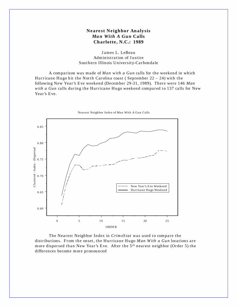
Nearest Neighbor Analysis Man With A Gun Calls Charlotte, N.C.: 1989

James L. LeBeau

Administration of Justice Southern Illinois University-Carbondale

A comparison was made of Man with a Gun calls for the weekend in which

Hurricane Hugo hit the North Carolina coast ( September 22 – 24) with the following New Year’s Eve weekend (December 29-31, 1989). There were 146 Man with a Gun calls during the Hurricane Hugo weekend compared to 137 calls for New Year’s Eve.

The Nearest Neighbor Index in CrimeStat was used to compare the distributions. From the onset, the Hurricane Hugo Man With a Gun locations are more dispersed than New Year’s Eve. After the 5th nearest neighbor (Order 5) the differences become more pronounced

0 5 10 15 20 25

ORDER

0.60

0.65

0.70

0.75

0.80

0.85

Clu

ster

ed -

Inde

x -

Dis

pers

ed

New Year's Eve WeekendHurricane Hugo Weekend

Nearest Neighbor Index of Man With A Gun Calls

5.11

sa ved as a ‘.dbf’ an d was t hen im por ted int o a gr aph ics pr ogra m. The graph shows t henearest neighbor indices for both robber ies and bu rgla r ies up t o the 50 t h order (i.e., the 50 t h

nearest neighbor ). The nearest neighbor in dex is sca led from 0 (ext reme clu ster in g) u p to 1(extr eme disper sion). Since a nearest neighbor index of 1 is expected u nder randomn ess,the th in st ra igh t line a t 1.0 in dica tes the expected K-order in dex. As can be seen , bothst reet robber ies and r esiden t ial burgla r ies a re much more concent ra ted t han K-orderspa t ia l r andomness. F ur ther , r obber ies a re more concent ra ted than even burgla r ies foreach of the 50 nea rest neighbors. Thu s, the gra ph reinforces t he ana lysis a bove th a trobber ies a re more concent ra ted t han bur gla r ies, an d both a re more concent ra ted t han arandom dis t r ibu t ion.

In other words, even t hough t here is not a good significance test for the K-ordernearest neighbor index, a gra ph of the K-order indices (or the K-order dist ances) can give ap ictu re of how clus tered the d is t r ibu t ion is a s well a s a llow compar isons in clus ter ingbetween the differen t types of crim es (or the same cr im e a t two differen t t im e per iods).

Gr a p h in g t h e K-or d er n ea r est n eig h bor

On the out pu t pa ge, ther e is a qu ick graph fun ction tha t displa ys a cur ve sim ilar tofigure 5.2. Th is is useful for qu ickly examining the t r en ds . However , a bet t er graph ismade by im por t ing the ‘dbf’ file ou tpu t in to a spr ea dsheet or gr aph ics progra m.

Edge Effec ts

It sh ould be noted tha t there are poten t ial edge effect s t ha t can bias the nearestneigh bor index. An inciden t occur r ing nea r the border of the s tudy a rea may actu a lly haveit s n ea rest neigh bor on t he other side of the border . However , sin ce ther e a re u su a lly noda ta on the dist r ibut ion of inciden t s out side t he st udy ar ea , th e pr ogra m select s a notherpoint wit h in the study a rea as t he nea rest neighbor of th e border point . Thus, t her e is t hepoten t ial for exaggera t ing the nearest neighbor dist ance, th a t is, th e obser ved nea restneighbor d ist ance is pr obably grea ter than wh at it sh ould be a nd, t her efore, ther e is a noverestim ation of the nea rest neighbor d ist ance. In oth er words , the inciden t s a re probablymore clus ter ed than wh at has been mea su red (see Cr essie , 1991 for deta ils).

N e a re s t N e ig h bo r E dg e Co rre c ti on s

The defau lt condit ion is no edge cor rect ion . However , one way th a t the measu reddis tance to the nearest neighbor can be corrected for possible edge effect s is to assume foreach obser ved point tha t there is an other poin t just ou t side t he border a t the closestdist ance. If the dist ance from a poin t to the border is shor ter than to its measu red n earestneigh bor, then the n ea rer theoret ical point is t aken as a pr oxy for t he n ea rest neigh bor. This cor rect ion has t he effect of redu cing the avera ge neighbor dist ance. Since it a ssu mestha t ther e is a lwa ys a noth er poin t a t the border , it pr obably un derestim ates t he t ruenearest neighbor dist ance. The t rue value is probably somewh ere in bet ween the measu redand t he assu med n earest neighbor dist ance.

5.12

Crim eS tat has t wo differen t edge cor rect ions. Because Crim eS tat is not a GISpackage, it cannot loca te the actua l border of a study a rea . One would need a topologica lGIS packa ge in wh ich t he dist ance from each point to th e n ea rest bounda ry is ca lcula ted. In st ead, th ere are two differen t geomet r ic models t ha t can be applied. The firs t assu mestha t the s tudy a rea is a rectangle wh ile t he second a ssumes tha t the s tudy a rea is a circle. Depen ding on the sh ape of the actua l study ar ea , one or eith er of these m odels m ay beappr opr iat e.

R ect a n gu la r st u d y a r ea

In the rectangula r adjus tment , th e area of the st udy ar ea , A, is fir st ca lcu lat ed,either from the user inpu t on the measurement pa rameters t ab or from the maximumboundin g rectangle defined by t he m in imum and m aximum X/Y values (see cha pt er 3). Ifthe user provides an est im ate of the a rea , t he rectangle is propor t ion a tely re-sca led so tha tthe area of the rectangle equa ls A. Second, for each poin t , th e dist ance to the nearest otherpoint is calcula ted. This is the obser ved n ea rest neighbor d ist ance for poin t i.

Third , th e minim um dist ance to the nearest edge of the rectangle is ca lcu lat ed a ndis compa red t o the obser ved nea rest neighbor dist ance for poin t i. If the obser ved nea restneighbor d ist ance for poin t i is equ a l to or less than the dist ance to the nea rest border , it isret a ined. On the oth er hand, if the obser ved n ea rest neighbor d ist ance for poin t i isgreat er th an th e dista nce to th e nearest border, th e dista nce to th e border is used as apr oxy for t he nea rest neighbor d ist ance of poin t i.

Ci r cu la r st u d y a r ea

In the cir cu la r adju stment , fir st , t he a rea of the study a rea is ca lcu la ted, eit her fromthe u ser inpu t on t he m ea su rem en t pa ramet er s t ab (see chapt er 3) or from the m aximumbounding recta ngle defined by th e minim um and m aximum X/Y values. If the user hasspecified a s tudy a rea on the measu remen t pa rameter s page, t hen tha t va lue is taken for Aand t he radius of the circle is ca lcu lat ed by

R = SQRT [A / B ] (5.8)

If the u ser has n ot specified a st udy a rea on t he m ea su rem en t pa ramet er s page, then A isca lcu la ted from the min imum and maximum X and Y coord ina tes (the bounding rectangle)and t he radius of the circle is ca lcu lat ed with equa t ion 5.8.

Second, for each poin t , the dist ance to the nea rest oth er point is calcula ted. This isthe obs erved nearest neighbor dis t ance for poin t i. Th ir d, for each poin t , i, t he dis t ancefrom t ha t point t o th e mean center is calculat ed, R i. Four th , the min imum d is tance to thenea rest edge of the circle is ca lcula ted usin g

R iC = R - Ri (5.9)

5.13

Fifth , for each poin t , i, th e obser ved minim um dist ance is compa red t o the nearestedge of the circle, RiC. If the obs erved nearest neighbor dis t ance for poin t i is equa l t o orless than the dis t ance t o the nearest edge, it is reta in ed. On the other hand, if theobserved nearest n eighbor dista nce for point i is great er th an th e dista nce to th e nearestedge, t he dis t ance to the border is used as a proxy for the t rue nearest neighbor dis t ance ofpoint i.

For eit h er cor r ect ion

The average nearest neighbor dis t ance is ca lcu la ted and compared to the theoret ica lavera ge nea rest neighbor dist ance under random condit ions. The indices a nd t est s a re asbefore (see chapter 4). F igure 5.3 below shows a gr aph of the K-order nearest neighborin dex for the 50 nearest neighbors for 1996 motor veh icle theft s in police Precin ct 11 ofBaltimore Coun ty. The uncorr ected near est neighbor indices are compa red with th osecor rected by a rectangle and a circle. As can be seen , both cor rections a re ver y sim ilar tothe uncor rected. However, th ey both sh ow grea ter concent ra t ions t han the uncor rectedindex. The recta ngular corr ection sh ows great er concentr at ion t ha n t he circular becau se itis less compact (i.e., the average dis t ance from the cen ter of the geomet r ic object to theborder is sligh t ly la rger ). In genera l, the rectangle will lead to more correct ion than thecircle sin ce it subst itu tes a grea ter nea rest neighbor d ist ance, on average, for a pointnearer the border than to it s measured nearest neighbor .

Th e u ser has t o decide wh et her eit her of these cor rect ions a re m ea ningful or not. Dependin g on t he shape of the s tudy a rea , eit her cor rect ion m ay or m ay not be a ppropr ia te. If the study a rea is rela t ively rectangu la r , t hen the rectangu la r model m ay provide a goodappr oximat ion . Similar ly, if the st udy ar ea is compa ct (circula r ), th en the circula r modelmay pr ovide a good approximat ion . On the oth er hand, if the study a rea is of ir r egu larsh ape, th en eith er of these cor rect ions m ay produce more dist or t ion than the raw nearestneighbor in dex. One has t o use t hese cor rections with judgemen t . Also, in some cases, itmay not m ake any sen se to corr ect the m ea su red nea rest neighbor d ist ances. In Honolulu ,for example, one wou ld not cor rect t he measu red nea res t neighbor dis t ances because thereare n o inciden t s ou t side t he is land’s boun da ry.

Linea r Nea rest Neighbor In dex (Lnna)

The linear nearest neigh bor index is a va r iat ion on the nearest neighbor rou t ine, butone applied to a s t reet network . All d is t ances a long th is network a re assumed to t r avela long a gr id, h en ce ind irect dis t ances a re u sed. Wh er ea s t he nea rest neighbor r out inecalculat es the distan ce between each point a nd its nea rest n eighbor u sing direct dista nces,the lin ea r nea rest neigh bor rout ine u ses in dir ect (‘Ma nha t tan’) dist ances (see chapt er 3). Similar ly, wher eas t he nearest neighbor rou t ine calcu lat es t he expected dist ance betweenneighbors in a random dist r ibut ion of N point s u sing th e geogra ph ica l ar ea of the st udyregion , t he linear nearest neighbor rout in e uses the tota l lengt h of the st reet network.

Correction of Nearest Neighbor IndicesMotor Vehicle Thefts in Precinct 11

Order

Nea

rest

nei

ghbo

r ind

ex

510

1520

2530

3540

45

1

0.9

0.8

0.7

Figure 5.3:

Random

Rectangular correction

Circular correction

No correction

Concentrated

Dispersed

5.15

Th e t heory of linea r nea rest neigh bors comes from Hammond and McCullagh(1978). The observed linea r nea rest neigh bor dis t ance, Ld(NN), is calcu la ted by Crim eS tatas t he avera ge of indirect d ist ances bet ween each poin t and it s n earest neighbor . Theexpected linea r nea rest neigh bor dis t ance is given by

LLd(ran) = 0.5 [------------------] (5.10)

N - 1

where L is th e tota l length of str eet n etwork an d N is the sam ple size (Ha mm ond a ndMcCullagh, 1978, 279). Consequent ly, th e linear n earest neighbor index is defined as

Linea r Nea res t Ld(NN)Neighbor Index = LNNI = --------------- (5.11)

Ld(ran)

Test ing the S igni fi cance o f the Linear Neares t Ne ighbor Index

Sin ce the theoret ica l s t andard er ror for the random linear nearest neighbor dis t anceis not known, t he au thor has const ructed an approximate st andard devia t ion for theobser ved linear nearest neighbor dist ance:

G ( Min(d ij) - Ld(NN) )2

SL d(N N ) . SQRT [ ------------------------------------ ] (5.12) N - 1

where Min(d ij) is the nearest neighbor dist ance for poin t i an d Ld(NN) is the avera ge linea rnearest neighbor dis t ance. This is the st andard devia t ion of the linear nearest neighbordist ances. The s t anda rd er ror is ca lcu lat ed by

SL d(N N ) SE L d(N N ) = -------------- (5.13)

SQRT[N]

An appr oximate significance test can be obta ined by

Ld(NN) - Ld(ran)t = ----------------------------- (5.14)

SEL d(N N )

where Ld(NN) is t he avera ge linea r nearest neighbor dist ance, Ld(ran) is the expectedlinea r nea rest neigh bor dis t ance (equ a t ion 5.10), and SE L d(N N ) is the approxima te s tanda rder ror of t he linea r nea res t neighbor dis t ance (equa t ion 5.13). Since the empir ica l s tanda rddevia t ion of th e lin ea r nea rest neigh bor is bein g used in st ea d of a t heoret ical va lue, t hetes t is a t-test r a ther t han a Z-t es t .

5.16

Calculating the s ta t is t i cs

On th e measu rem ents pa ra met ers page, th ere ar e two par am eters t ha t a re input ,the geogr aphica l a rea of the study r egion and the lengt h of st reet network. At the bot tomof the page, t he user must select wh ich type of d is t ance measu remen t t o use, d ir ect orind irect . If the measurement type is direct , then the neares t neighbor rou t ine retu rns thesta nda rd n earest neighbor a na lysis (somet imes called areal nea rest neighbor ). On theother hand, if t he measu remen t t ype is indir ect , t hen the rou t ine r etu rns the linea r nea res tneighbor ana lysis . To ca lcu la te the linear nearest neighbor in dex, therefore, d is t ancemeasu rement must be specified as indirect and t he length of the st reet network m ust bedefined.

Once nearest neighbor ana lysis has been selected, t he user clicks on Com pute t o runthe rou t ine. The Lnna rout ine out put s 9 stat istics:

1. Th e sample size2. The mean linear nearest neighbor dist ance 3. The minimum linear distan ce between n earest neighbors 4. The maximum linear dis t ance between nearest neighbors5. The mean linear random dist ance 6. Th e lin ea r nea rest neigh bor index 7. The st anda rd deviat ion of the linear nearest neighbor dist ance 8. The standard er ror of the linear nearest neighbor dis tance9. A significance test of the nearest neighbor index (t -t est )10. The p-va lues associat ed with a one ta il and t wo ta il significance test .

Example 3: Auto theft s a long tw o h ighw ays

The linea r nea rest neighbor in dex is u seful for ana lyzing t he dist r ibu t ion of crim einciden t s a long pa r t icula r st r eet s. F or exa mple, in Ba lt imore Coun ty, st a te h ighwa y 26 inthe western par t and sta te h ighway 150 in the eastern par t have h igh concent ra t ion s ofmotor vehicle th eft s (figure 5.4). In 1996, th ere were 87 vehicle th eft s on h ighway 26 an d47 on h ighway 150. A GIS can be used wit h the linear nearest neighbor in dex t o in dica tewh et her these in ciden t s a re gr ea ter than wh at would be expected on t he ba sis of cha nce.

Table 5.3 pr esen t s t he da ta . Using th e GIS, we est ima te tha t there are 3,333.54miles of roadway segm ents; th is number was es t im ated by addin g u p the tota l lengt h of thest reet network in the GIS. Of a ll the road segm ents in Balt imore Coun ty, there are 241.04miles of major a r t er ial r oads of which st a te h ighway 26 ha s a tota l length of 10.42 milesand s ta te h ighwa y 150 has a tota l road len gth of 7.79 miles .

In 1996, there were 3,774 motor vehicle th eft s in the county. If these t heft s wer edist r ibut ed r andomly, then the random expected dist ance between inciden t s would be 0.44miles (equa t ion 5.10). Using th is est ima te, ta ble 5.3 sh ows t he number of inciden t s t ha twould be expected on each of the two sta te h ighways if t he dis t r ibu t ion were random andthe ra t io of the actua l nu mber of motor vehicle th eft s t o the expected n umber . As can be

Miles

420

Figure 5.4:

1996 Auto Thefts in Baltimore CountyIncident Distribution on State Highways 26 and 150

State Highway 26

State Highway 150

5.18

Ta ble 5.3

Compar ison of 1996 Ba lt imore County Au to Theftsfor Differen t Types of Roads

(N = 3774 Incidents)

Length of Road Segment s:

Highway 26 10.42 miHighway 150 7.79 miAll MajorAr ter ia ls 241.04 miAll Roads 3333.54 mi

Random E xpected Dist ance Between Incident s = 0.44 miles

Propor t iona l To Network Proport iona l to Sa me Road

Avera ge “Rela t ive

“Rela t ive Avera ge R a n d om t o I t se lf”

t o R a n d om ” Linea r Linea r Linea r

Wh e r e N u m b e r E x p e c te d N e a r e s t N e a r e s t N e a r e s t

I n c i d e n t s o f N u m b e r R a t io o f N e i g h b o r N e i g h b o r N e i g h b o r

O c c u r r e d I n c i d e n t s If R a n d o m F r e q u e n c y D i s ta n c e D i s ta n c e In d e x

Highway 26 87 11.8 7.4 0.05 mi 0.06 0.96

Highway 150 47 8.8 5.3 0.08 mi 0.08 0.94

All MajorAr ter ia ls 607 272.8 2.2 0.13 mi 0.20 0.64

(p#.001)

All Roads 3774 3774.0 1.0 0.09 mi 044 0.21(p#.001)

5.19

seen , th e dist r ibut ion of motor vehicle th eft s is not random. On a ll major a r t er ial r oads, t hereare 2.2 t im es as many t heft s as would be expected by a random spa t ia l d is t r ibu t ion . In fact ,in 1996, of 28,551 road segm ents in Ba lt im ore Cou nty, only 7791 (27%) had one or more motorveh icle t heft s occu r on them; mos t of t hese a re ma jor roads . Fu r ther , on h ighway 26 therewere 7.4 times a s m uch and on h ighway 150 th ere were 5.3 times a s m uch as would beexpected if the dist r ibu t ion wa s r andom. Clea r ly, th ese t wo high wa ys h ad m ore t han theirsh are of au to th efts in 1996.

But wha t a bout th e distr ibut ion of th e incidents along each of th ese highwa ys? Ifthere were any pa t t ern , for exa mple, m ost of the in ciden t s clu ster in g on the western edge orin t he cen ter , th en police could use t ha t informat ion to more efficient ly deploy vehicles torespond quickly to event s. On t he other hand, if the dist r ibut ion a long th ese h ighways wereno differen t than a random dist r ibut ion , th en police vehicles must be posit ioned in t he middle,since tha t would minim ize the dist ance to a ll occur r ing incident s.

Unfor tuna tely, t he r esu lt s a ppea r to be close to a r andom dis t r ibu t ion. Crim eS tatca lcu lat es t ha t for h ighway 26, the avera ge linea r nearest neighbor dist ance is 0.05 mileswh ich is close t o th e average random linea r nea rest neighbor d ist ance (0.06 m iles). The r a t io- th e linea r nea rest neighbor in dex, is 0.96 with a t -va lue of -0.16, which is not s ignifican t lydifferen t from chance. Sim ila r ly, for h ighway 150, t he average linear nearest neighbordist ance is 0.079 miles which , aga in, is a lmost ident ica l to th e avera ge ra ndom linea r nearestneighbor dist ance (0.084 miles); the nearest neighbor index is 0.94 an d t he t -value is -0.41(not significan t). In short, even th ough th ere was a h igher concentr at ion of vehicle th efts onthese two sta te h ighways than would be expected on the basis of chance, t he dis t r ibu t ionalong each h ighway is n ot very differen t than what would be expected on the bas is of chance.5

K-Order Linear Nearest Neighbors

There is also a K-order linear near est neighbor a na lysis, as with t he ar eal nearestneigh bors. The u ser can specify how many add it iona l nea rest neigh bors a re t o be calcu la ted. The linea r K-order nea rest neighbor r out ine r et urns four columns:

1. The order , s t a r t in g fr om 12. The mean linear nearest neighbor dist ance for each order (in m eters)3. The expected linea r nearest neighbor dist ance for each order (in m eters)4. The linear nearest neighbor index for each order

Since the expected linea r nearest neighbor dist ance has n ot been work ed out for order s h igher than one, t he ca lcu la t ion produced here is a rough approximat ion . I t applies equa t ion5.10 only a dju st ing for the decrea sin g sa mple size, N k , which occurs as degr ees of freedom arelost for each successive order. In th is sense, th e index is really th e k-order linear near estneighbor dis t ance rela t ive to the expected linear neighbor dis t ance for the fir st order . I t is nota st r ict nearest neighbor index for order s a bove one.

Never theless, like t he area l k-order nearest neighbor index, the k-order linear nearestneighbor index can pr ovide ins igh t s in to the dist r ibut ion of the poin t s, even if the firs t -order

5.20

is r andom. Figure 5.5 shows a graph of 50 linea r nea rest neighbors for 1996 residen t ia lburgla r ies and st reet robber ies for Balt imore Coun ty. As with the area l k-order nearestneighbors (see figure 5.3) both burgla r ies and robber ies show evidence of clu ster in g. For both ,the firs t nearest neighbors a re closer togeth er than a random dist r ibut ion . Similar ly, over t he50 orders, s t r eet robber ies a re more clu stered than burgla r ies. H owever , m easur in g dis t anceon a gr id shows tha t for bu rgla r ies, t here is only a small amount of cluster in g. After thefour th order n eighbor, the distribution for bur glaries is more dispersed th an a r an domdis t r ibu t ion . An in terpreta t ion of th is is tha t there a re small number of bu rgla r ies which areclus ter ed, bu t the clust er s a re r ela t ively disper sed. S t reet robber ies , on t he other hand, a rehighly clustered, up t o over 30 near est neighbors.

Th e lin ea r k-order nea rest neigh bor dis t r ibu t ion gives a sligh t ly differen t perspect iveon t he distribution t ha n t he ar eal. For one th ing, th e index is slight ly biased as t hedenomin a tor - the K-order expected linear neighbor dis t ance, is only approximated. F oranother th ing, th e index m easu res dist ance as if the st reet follow a t rue gr id, orien ted in aneast -west and n or th-sout h direct ion . In t h is sen se, it m ay be un rea listic for many places,especia lly if st r eet s t r averse in dia gon a l pa t terns; in these cases, t he use of in dir ect dis t ancemea su rem en t will pr oduce grea ter dis t ances t han wh at actu a lly occur on t he net work. St ill,the linear nearest neighbor index is a n a t t empt to appr oximate t r avel a long th e st reetnet work. To the ext en t tha t a pa r t icula r jur isd iction’s s t reet pa t t er n fall in th is m anner , itcan provide usefu l in format ion .

Gr a p h in g t h e li n ea r K-ord er n ea r est n eig h bor

On the out pu t pa ge, ther e is a qu ick graph fun ction tha t displa ys a cur ve sim ilar tofigur e 5.5 below. Th is is useful for qu ickly exa min ing the t r en ds .

Ripley’s K S ta t ist ic

R ipley’s K st a t ist ic is an index of non-randomness for differen t sca le va lues (Ripley,1976; Ripley, 1981; Ba iley and Gat t rell, 1995; Ven ables and Rip ley, 1997) . In th is sen se, it isa ‘super -order ’ nearest neighbor st a t is t ic, providin g a test of randomness for every dis t ancefrom the sm allest u p t o some specified limit. a rea . It is somet imes ca lled th e reduced secondm om ent m easu re, implyin g t ha t it is designed to measure second-order t r ends (i.e., loca lclus ter ing as opposed to a gen er a l pa t t er n over the r egion). However , it is a lso su bject t o fir st -order effect s so tha t it is not st r ict ly a second-order measu re.

Consider a spatially random dis t r ibu t ion of N point s. I f cir cles of r adiu s, t s, ar e drawnaroun d each point , wh er e s is t he order of radii from t he smalles t to th e la rgest , and t henumber of oth er point s t ha t a re found with in the circle a re counted and t hen su mmed over a llpoint s (a llowin g for duplicat ion), then the expected number of point s with in tha t radiu s a re

K-Order Linear Nearest Neighbor Indices1996 Street Robberies and Residential Burglaries

Order of Linear Nearest Neighbor Index

Line

ar N

eare

st N

eigh

bor I

ndex

05

1015

2025

3035

4045

4.5

4

3.5

3

2.5

2

1.5

1

0.5

0

Figure 5.5

K-order spatial randomness

Residential burglaries

Street robberies

5.22

NE(# of poin t s with in d ist ance d i) = --------- K(t s) (5.15)

A

where N is the sample size, A is the tota l s tudy a rea , a nd K(t s) is the area of a circle definedby r adiu s, t s. F or exa mple, if the a rea defin ed by a par t icu la r radiu s is one-four th the tota lstu dy ar ea an d if there is a spa t ially ra ndom dist r ibut ion , on avera ge app roximately one-four th of the cases will fa ll wit h in any on e cir cle (plu s or min us a sampling er ror ). Moreformally, with com plete spatia l ran dom ness (cs r ), the expected number of poin t s with indis tance, t s, is

NE(# un der csr ) = ------ B t s

2 (5.16) A

On the other hand, if the average number of poin t s found wit h in a cir cle for apa r t icu lar radius pla ced over each poin t , in tu rn , is grea ter than tha t found in equa t ion 5.16,th is poin t s to clu ster in g, tha t is poin t s a re, on average, closer than would be expected on theba sis of cha nce for t ha t radiu s. Conver sely, if the average number of points found with in acircle for a par ticular ra dius placed over each point, in t ur n, is less tha n t ha t foun d inequa t ion 5.16, th is poin t s t o disper sion ; tha t is point s a re, on avera ge, fa r ther apa r t thanwould be expected on the basis of chance for tha t radiu s. By cou nt in g t he number of tota lnumbers wit h in a par t icu la r radiu s and compar in g it to the number expected on the basis ofcomplete spa t ia l randomness, t he s t a t ist ic is an indica tor of non-ra ndomness.

In th is sen se, the K s ta t ist ic is s imilar to th e nea rest neighbor d ist ance in t ha t itprovides in format ion about the average dis t ance between poin t s. H owever , it is morecomprehens ive than the neares t neighbor s t a t is t ic for two reasons . F ir s t , it applies to a llorder s cumula t ively, not jus t a sin gle order . Second, it app lies t o all dist ances up t o th e limitof the study a rea because the count is condu cted over su ccessively in creasin g radii.

Un der un const ra ined conditions, K is defined as

A

K(t s) = ------ G G I (t ij) (5.17)

N 2 i i=/ j

where I(t ij) is t he n umber of oth er poin t s, j, found with in dis t ance, t s, sum med over all points,i. Tha t is, a circle of radiu s, t s, is placed over each poin t , i. Then , the number of oth er point s,j, with in the circle is counted. The circle is m oved t o th e n ext i and t he process is repea ted. Thus, t he double summat ion poin t s to the count of a ll j’s for each i, over a ll i’s. Note, t he countdoes not include it self, on ly oth er poin t s.

After th is process is completed, the r adiu s of the circle is in creased, a nd t he en t ireprocess is repea ted. Typica lly, the radii of cir cles a re in creased in small in crements so tha t

5.23

ther e a re 50-100 in ter va ls by wh ich t he s t a t ist ic can be coun ted. In Crim eS tat, 100 in ter vals(radii) a re used, based on

Rt s = -------- (5.18)

100

where R is th e radius of a circle for whose a rea is equa l to th e st udy ar ea (i.e., the areaen tered on the measurement parameter s page).

One can gra ph K(t s) aga inst the dist ance, t s, to revea l whet her ther e is a ny clust er inga t cer t a in d ist ances or any disper sion a t others (if there is clus ter ing a t some scales, thenther e m ust be disper sion a t oth er s). Su ch a plot is n on-linea r , however , typically increa sin gexponent ia lly (Kalu zn y et a l, 1998. Consequent ly, K(t s) is t r ansformed in to a square rootfunct ion , L(t s), t o make it more linear . L(t s) is defined as:

K(t s)L(t s) = SQRT [ --------- ] - t s (5.19)

B

Th at is , K(t s) is divided by B and then the square root is t aken . Then the dis t ancein terva l (the pa r t icu la r r ad ius ), t s, is subtr acted from t his.6 In pr actice, on ly the L s ta t ist ic isused even though the n ame of the s t a t ist ic K is ba sed on the K der iva t ion.

Because the L(t s) is a measure of second-order clu ster in g, it is usua lly a na lyzed foronly a sh ort distan ce. In Crim eS tat III, th e dist ance is set a t one-th ird the side of a squ aredefin ed by the a rea (SQRT[A]/3).7 Figure 5.6 shows a gra ph of L(t ) against dist ance for 1996robber ies in Ba lt im ore Cou nty. As can be seen , L(t ) in creases up to a dis t ance of about 3miles whereu pon it decreases a gain. A “pu re” ra ndom dist r ibut ion , known as com plete spatialran dom ness (CSR), is sh own as a hor izonta l line a t L=0.

Comparison to A Spat ia lly Random Dis tribut ion

To understand whether an obs erved K dis t r ibu t ion is differen t from chance, on etypica lly u ses a random dis t r ibu t ion . Because the sampling dis t r ibu t ion of L(t s) is not kn own,a simulat ion can be condu cted by ra ndomly ass ign ing poin t s t o the st udy ar ea . Because a nyone s imula t ion migh t p roduce a clus tered or d ispersed pa t t ern s t r ict ly by chance, thesim ula t ion is repea ted many t im es, t yp ica lly 100 or more. Then , for each random sim ula t ion ,the L st a t ist ic is ca lcu lat ed for each dist ance int erval. Fina lly, after a ll simulat ions h ave beenconducted , the h ighes t and lowes t L-va lues a re t aken for each d is tance in terva l. Th is is ca lledan envelope. Thu s, by compa r ing the dist r ibut ion of L to th e random en velope, one can asses swhether the pa r t icu lar obser ved pa t t ern is likely to be differen t from chance.8 In figure 5.6,the L en velope of random da ta is m uch less concent ra ted than tha t for robber ies, indicat ingtha t it is h igh ly un likely the concent ra t ion of robber ies was du e to chance.

"K" Statistic For 1996 RobberiesCompared to Random and 2000 Population Distributions

L(t) = Sqrt[K(t)/pi] - t

Figure 5.6:

0.1 1.4 2.7 4.0 5.3 6.6 7.9

Distance between points(miles)

-2

-1

0

1

2

3

L(t)

Robbery

Population

CSR

Envelope of 100 random simulations

5.25

S pe c ify in g si m u la ti on s

Because s imula t ions can t ake a long t ime, pa r t icu la r ly if the da ta set s a re la rge, thedefau lt number of sim ula t ions is 0. However , a user can condu ct s imula t ions by wr it ing aposit ive n umber (e.g., 10, 100, 300). If sim ula t ions a re select ed, Crim eS tat will con duct thenumber of sim ula t ion s specified by t he user and will ca lcu la te the upper and lower limit s foreach dist ance int erval, as well a s t he 0.5%, 2.5%, 5%, 95%, 97.5% and 99% int ervals; th esela t t er st a t ist ics only m ake sen se if ma ny sim ula t ion r uns a re condu cted (e.g. 1000).

Th e wa y Crim eS tat conduct s the s imula t ion is a s follows . It t akes the maximumbounding rectangle of the d is t r ibu t ion , tha t is the rectangle formed by the maximum andminimum X and Y coordin a tes respectively a nd r e-scales t h is (up or down) un t il the r ectanglehas a n area equa l to th e st udy ar ea (defined on the measu rement pa rameters pa ge). It t henass igns N point s, wh er e N is t he same number of point s a s in the inciden t dis t r ibu t ion , usin ga un iform random n umber gener a tor to th is rectangle and calcu lat es t he L st a t ist ic. It t henrepea t s t he exper imen t for the n umber of specified simula t ions , and ca lcula tes the a bovest a t ist ics. For example, with 1181 robberies for 1996, the Ripley’s K fun ct ion ca lcu lat es t heempir ica l L sta t ist ics for 100 dist ance int ervals a nd compa res t h is to a simulat ion of 1181poin t s r andomly distr ibut ed over a rectangle k t imes , wher e k is a user -defined n umber .

In pr act ice, th e simulat ion test a lso has biases a ssociat ed with edges. Un like thetheoret ical L u nder un iform condit ions of complete spa t ia l randomness (i.e., st r et chin g in a lldirect ions well beyond t he st udy ar ea) where L is a s t ra igh t hor izonta l line, the simulat ed La lso declines wit h in creasin g dis t ance separa t ion between poin t s. This is a funct ion of thesa me t ype of edge bia s.

Co m pa ri so n to B as e li ne P o p u la ti on s

For most social dist r ibut ions, such as crime inciden t s, randomn ess is n ot a verymea ningfu l baseline. Most socia l character ist ics are non-random. Consequ en t ly, to find tha tthe amoun t of clust er ing tha t is occur r ing is gr ea ter than wh at would be expected on t he ba sisof chance is not very useful for cr ime a na lyst s. However, it is possible to compa re thedis t r ibu t ion of L for crim e inciden t s with the dist r ibu t ion of L for var ious baselinecha racter ist ics, for exa mple, for the popu la t ion d ist r ibu t ion or the dist r ibu t ion of employmen t . In a lmost a ll met ropolita n a reas, popu lat ion is more concent ra ted t owards t he cen ter than a tthe per iph er y; the drop-off in popu la t ion densit y is ver y sh arp a s was shown in the la stchap ter . All other th ings being equa l, one would expect more inciden t s towards themet ropolita n cen ter than a t the per iphery; consequ ent ly, th e avera ge dista nce betweeninciden t s will be shor ter in the cen ter than fa r ther ou t . Th is is noth ing more than aconsequence of the dis t r ibu t ion of people. H owever , t o say somethin g a bout concent ra t ion s ofin ciden t s above-and-beyon d tha t expected by popula t ion requir es us to exa min e the pa t t ern ofpopulat ion a s well as of crime incidents.

Crim eS tat a llows the use of in tensit y a nd weight in g va r ia bles in the calcu la t ion of theK st a t ist ic. The user must define an int ensity or a weight (or both in special circum st ances)on t he pr imary file pa ge. The K r out ine will t hen use the in ten sit y (or weigh t ) in the

5.26

ca lcu la t ion of L. In Figure 5.6 above, t here is an envelope produced from 100 randomsimu lat ions a s well as the L distr ibut ion from the 2000 popu lat ion ; the lat t er va r iable wasobta ined by taking the cent roid of t r a ffic ana lysis zones from the 2000 censu s a nd u sin gpopu la t ion as t he in ten sit y var iable. As can be seen , the amoun t of clust er ing for r obber ies isgrea ter than both the random en velope a s well as the dist r ibut ion of popula t ion . The robberyfunct ion is h igher than the popula t ion funct ion up to abou t 6 miles . Th is ind ica tes tha trobber ies a re more concent ra ted than what would be expected from the popula t iondis t r ibu t ion for a fair ly la rge a rea .

In other words, r obber ies a re more clus tered t ogeth er than even wh at would beexpected on the basis of t he popula t ion dis t ribu t ion and th is holds for dis t ances up to abou t 6miles, whereupon the dis t r ibut ion of robber ies is in dis t in gu ishable from a randomdis t r ibu t ion . For la rger dis t ance separa t ions, t he L function has lit t le u t ility sin ce it isusually u sed to understand loca lized spa t ia l a u tocorrela t ion (Ba iley a nd Gat t rell, 1995).

For compa r ison, figure 5.7 below shows t he dist r ibu t ion of 1996 bu rglar ies, againcompared to a r andom envelope and the d is t ribu t ion of popula t ion . We find tha t bu rgla r iesa re more clu stered than popula t ion , bu t less so than for robber ies; the L va lu e is h igher forrobberies th an for bur glaries for n ear dista nces but becomes more dispersed at a bout 3 miles;it is still more concentr at ed tha n a ra ndom distr ibut ion, however, as seen by th e ran domenvelope.. Thus, the dist r ibut ion of L confirm s t he resu lt t ha t bur gla r ies tend t o be spr eadover a much la rger geograph ica l a r ea in sma ller clust er s t han st r eet robber ies , wh ich t end tobe more concen t r a t ed in la rge clust er s . In t erms of look ing for ‘hot spot s ’, one wou ld expect t ofind more with robberies th an with burglar ies.

Edge Correct ions for Rip ley’s K

The L s ta t ist ic is prone t o edge effects ju st like the nea rest neighbor s t a t ist ic. Tha t is,for poin t s loca t ed nea r t he boundary of t he s tudy a rea , t he number enumera ted by any cir clefor those point s will, a ll other th ings being equa l, necessa r ily be less than poin t s in the cen terof t he s tudy a rea because poin t s ou t side the boundary a re not coun ted . Fu r ther , t he grea t erthe dist ance between point s t ha t a re bein g tested (i.e., the grea ter the r adiu s of the circleplaced over each point ), th e grea ter t he bias. Thus, a plot of L aga inst distance will show adeclin ing curve as dist ance increases a s figures 5.6 and 5.7 show.

Th er e a re va r ious adju st men ts t o th e function to help corr ect the bia s. One is a ‘guardra il’ wit h in the study a rea so tha t poin t s out side the gu ard ra il, bu t in side the study a rea canonly be coun ted for poin t s ins ide the guard ra il, bu t cannot be used for enumera t ing otherpoin t s with in a circle placed over them (tha t is, th ey can on ly be j’s a nd n ot i’s, to use t helanguage of equ a t ion 5.17). Such a n opera t ion , however , requ ires manua lly cons t ructin gthese gu ard ra ils and enumera t in g whether each poin t can be both an enumera tor and arecip ien t or a recip ien t only. F or complex boundar ies, such as a re found in most policedepa r tmen ts, t h is t ype of opera t ion is ext rem ely tedious a nd d ifficult .9

0.09 1.39 2.7 4.0 5.3 6.6 7.9

Distance between points (miles)

-2

-1

0

1

2

3

L(t)

Population

Burglary

CSR

Envelope of 100 random simulations

"K" Statistic For 1996 BurglariesCompared to Random and 2000 Population Distributions

L(t) = Sqrt[K(t)/pi] - t

Figure 5.7:

5.28

Sim ila r ly, Ripley h as proposed a sim ple weight in g t o account for the propor t ion of thecircle placed over each poin t tha t is with in t he st udy ar ea (Venables an d Ripley, 1997). Thu s,equa tion 5.17 is re-written as:

A

K(t s) = ------ G G Wij-1 I (t ij) (5.20)

N 2 i j

where Wij-1 is t he in ver se of the proport ion of th e circum feren ce of a circle of ra diu s, t s, placed

over each poin t t ha t is with in the tot a l s tudy a rea . Thus, if a poin t is nea r t he s tudy a reaborder , it will r eceive a grea ter weigh t because a sm aller pr opor t ion of the circle pla ced over itwill be wit h in the study a rea . An a lt erna t ive weight in g scheme can be found in Marcon andPuech (2003).

In Crim eS tat, two possible corr ections a re condu cted. One assum es tha t t he stu dyarea is a r ectangle while the other assu mes t ha t it is a circle.

R ect a n gu la r cor r ect ion

In the r ectangula r cor rect ion for Ripley’s K, the sea rch cir cle radiu s, R j, is compa red tothe edge of an assu med r ectangle with a rea , A, cen tered a t the mean center . Fir st , th e area tobe an alyzed is defined . If the user has specified a st udy ar ea on the measu rement pa rameterspa ge, t hen tha t va lue for A is t aken . The m aximum boundin g rectangle is t aken (i.e.,r ectangle defined by th e minim um and m aximum X/Y values) an d pr oport iona tely re-scaled sotha t the a rea of the rectangle is equa l t o A. If the user does not specify an area on themea su rem en t pa ramet er s page, then the boundin g rectangle defined by the m inimum andmaximum X/Y va lues is taken for A.

Second, for each poin t , the m inimum dis tance to the nea rest edge of th is r ectangle iscalcula ted in both the horizonta l and ver t ical directions, d(min RX) and d (minRY). Th ir d, eachof th e minimu m dista nces is compa red to th e sear ch circle ra dius, Rj.

1. If neit her the m inimum dis tance in t he X-dir ection - d(minRX), nor theminimum dis tance in t he Y-dir ection - d(minRY), a re less t han the sea rch circlera dius, Rj, th en the circle fa lls ent irely with in t he rectangle and E = 1;

2. If either the m inimum dis tance in t he X-dir ection - d(minRX), or the min imumdis tance in t he Y-dir ection - d(minRY), bu t NOT BOTH, a re less than the searchcircle r adiu s, R j, th en par t of th e sear ch circle falls out side the recta ngle and a nadjust men t is n ecessa ry. An approximate adjust men t is m ade than is in ver selypropor t ion a l t o the a rea of the search cir cle wit h in the rectangle. The va lu es ofE will vary bet ween 1 and 2 s ince up to one-ha lf of the sea rch circle could fallou t s ide the rectangle;

3. If both the m inimum dis tance in t he X-dir ection - d(minRX), and the min imumdis tance in t he Y-dir ection - d(minRY), ar e les s t han the sea rch cir cle radiu s, R j,

5.29

then a gr ea ter adju stment is requir ed sin ce E could va ry between 1 and 4 sin ceup t o th ree-four th of the sea rch circle could fa ll ou t side t he rectangle.

The formulas used t o ca lcu lat e the rectangula r weight s a re:

R adius does not extend beyond the rectangle:

Wij-1 = k = 1 (5.21)

R adius extends beyond one edge of the rectangle (bu t not two):

2B Wij

-1 = k = { ----------------------------------------- } (5.22) {2B - 2Cos-1[d(min R)/Ri]}

R adius extends beyond two edges of the rectangle:

2 B Wij

-1 = k = { ------------------------------------------------------------------ } (5.23) {1.5B - Cos-1[d(min Rx)/Ri]-Cos-1[d(min Ry)/Ri]}

While in tu it ive, t h is weigh t , Wij-1, is p rone to cause upward ‘dr ift’ in the K function , so

a log tr an sform at ion is used:

W’ij

-1 = ln (Wij-1) + 1 (5.24)

This h as t he effect of t emper ing th e dr ift somewha t .10

Ci r cu la r cor r ect ion

In the circula r cor rect ion for Ripley’s K, the sea rch cir cle radiu s, R j, is compared to theedge of an assu med circle with a rea , A, cen tered a t the mean center . Fir st , th e area to beana lyzed is defined . If the user has specified a st udy ar ea on the measu rement pa rameterspa ge, t hen tha t va lue for a is t aken . The r adiu s of th e circle, Rj, is ca lcula ted by equa t ion 5.8above. If the user has n ot specified a st udy ar ea on the measu rement pa rameters pa ge, thenA is ca lcu la t ed from the maximum bounding r ect angle and the r adius of t he cir cle isca lcu lat ed by equa t ion 5.8 above.

Second, for each point , the dist ance from t ha t poin t to th e m ea n center , R j, isca lcu lat ed. The n earest dist ance from the poin t to the circle’s edge is given by

R jC = R - Rj (5.25)

5.30

Th ird, t he sea rch cir cle radiu s, R j, is compared to th e n ea rest edge of the circle, RiC,and t he weight will var y from 1 (poin t and r adius t ota lly with in t he st udy ar ea) to 2.3834(poin t is loca ted exa ct ly on boundary of a rea cir cle). The formula s for the cir cu la r correct ionare:

2 = Cos-1 {(r 2 + t C2 - R2) / [ 2*r *t C ]} (5.26)

Wij-1 = k = B / 2 (5.27)

where r is t he r adiu s of th e sea rch cir cle, R is t he r adiu s of th e circula r st udy a rea , and t C isthe dist ance from the poin t to the cen ter of the circula r st udy ar ea .

For eit h er cor r ect ion

Dur in g t he ca lcu la t ion of Ripley’s K, each poin t is mult ip lied by E (aside from W or I)and the K and L sta t is t ics a re ca lcu la ted as before (see chapter 5). The sim ula t ion of randompoin t dis t r ibu t ions is t r ea ted in an ana logous way.

While in tu it ive, t h is weigh t , Wij-1, is p rone to cause upward ‘dr ift’ in the K function , so

a log tr an sform at ion is used:

W’ij

-1 = ln (Wij-1) + 1 (5.28)

This h as t he effect of t emper ing th e dr ift somewha t .

F igure 5.8 below sh ows a Ripley’s K dist r ibut ion for 1996 Balt imore Coun ty bur gla r ies,with and without edge cor rect ions. As can be seen , th e uncor rected L dist r ibut ion decrea sesand fa lls below the theoret ica l r andom count (complete spa t ia l r andomness, L=0) a ft er about7 miles wher eas n eith er the L dist r ibut ion with the rectangula r cor rect ion nor the Ldis t r ibu t ion wit h the cir cu la r dis t r ibu t ion do so. As expected, t he rectangu la r dis t r ibu t ionproduces the mos t concen t ra t ion .

Output Inte rme diate Res ults

Ther e is a box labeled “Ou tpu t in ter media te r esu lt s”. If checked, a sepa ra te dbf filewill be ou tpu t tha t list s t he int ermedia te ca lcu lat ions. The file will be ca lled“RipleyTempOu tpu t.dbf”. There are five out put fields:

1. Th e point number (POIN T), st a r t ing a t 0 (for t he first poin t ) an d p roceed ing toN–1 (for t he Nth poin t )

2. The sear ch r adius in m eters (SEARCHRADI)3. The coun t of t he number of other point s t ha t a re wit h in the sea rch r adiu s

(COUN T)4. The weight assigned, ca lcu lat ed from equa t ions 5.24 or 5.28 above (WEIGHT)5. The count t imes the weight (CTIME SW)

"K" Statistic For 1996 BurglariesWith Different Types of Corrections

L(t) = Sqrt[K(t)/pi] - t

Figure 5.8:

0.09 1.39 2.7 4.0 5.3 6.6 7.9

Distance between points (miles)

0

1

2

3

4

L(t)

No correction

Rectangular correction

Circular correction

K-Function Analysis to Determine Clustering in the Police Confrontations Dataset in

Buenos Aires Province, Argentina: 1999

Gastón Pezzuchi, Crime Analyst Buenos Aires Province Police Force

Buenos Aires, Argentina

Sometimes crime analysts tend to produce beautiful hot spot maps without any formal evidence that clustering is indeed present in the data. One excellent and powerful tool that CrimeStat provides is the computation of the K function, which summarizes spatial dependence over a wide range of scales, and uses the information of all events.

We computed the K function using 1999 police confrontations data (mostly

shootings) within our study area1 and ran 100 Monte Carlo simulations in order to test for spatial randomness2 (see figure below); the K function showed clustering up to about 30 Km. Yet, spatial randomness is not a particularly meaningful hypothesis to test considering that the “population at risk” are highly clustered. Hence we used police deployment data as a base population and calculated the K function for that data set. As can seen, the amount of clustering for the confrontation dataset is much greater than both the random envelope as well as the distribution of police officers.

Distance Between Points [km]

0 10 20 30 40

L(d)

-12

-10

-8

-6

-4

-2

0

2

4

6

L(d)CSRL(d)_MINL(d)_MAX L(d) Base Population

K Statistic for the 1999 DatasetL(d) = Sqrt[K(d)/π] - d

Observed L(d)

100 Sim. Envelope

Base-Population L(d)

1 A years worth dataset of events occurring within a 9,500 km2 area around the Federal Capital (29 counties). 2 Remember that Pr( L(d) > Lmax) = Pr( L(d) < Lmin) = 1 / (m + 1) where m is the number of independent simulations,

5.33

This outpu t can be usefu l for exa min in g t he counts for specific poin t s or for t rying ou taltern at ive weight ing schemes.

Some Caut ions in Us ing Rip ley’s K

While Ripley’s K is a power ful t ool for a na lyzing spa t ia l au tocorr ela t ion (usua llyclus ter ing, ra ther than disper sion), like a ny sta t ist ic it is pr one to biases. We’ve discussededge bia ses a bove. But ther e a re oth er s. F ir st , ther e is a sa mple size issu e. The r out inecalcu la tes 100 separa te L(t ) va lu es, one for ea ch dis t ance bin . H owever , t he precis ion of anyone L(t ) va lue is dependen t on the sample s ize. With a sma ll s ample, t here is in su fficien t da t ato est im ate 100 in dependent va lu es of L(t ). While the Monte Ca r lo s im ula t ion par t ly canaccoun t for tha t bia s, it has t o be rea lized tha t the precision of the in ter pr et a t ion is su spect . For exam ple, in compa r ing two similar dist r ibut ions, say robberies and bu rgla r ies, un less t hesa mple size is la rge differences for any one bin could easily be due to chance. One would needa very differ en t type of procedure t o est imate t he ‘st anda rd er ror’ of two functions with a sm allsa mple. But , I would su spect t ha t there would be ma ny bins for which they would beindis t inguish able (shown as t he t wo fun ctions cr iss -crossing ea ch other ).

In previous version s of Crim eS tat, ther e wa s a rest r iction of a t lea st 100 da ta point s t odispla y th e ent ire 100 L(t) est ima tes; otherwise, th ey were t runca ted. In th is version, all 100inter vals a re a llowed for any size sample. However , ther e is a st r ict wa rn ing. User s shouldbe ver y cau t ious in dr awin g conclusions a bout differ en ces in the L function wit h sm allsa mples. E ven wit h sa mple sizes grea ter than 100, t he impr ecision of any one L(t) va lue isconsider able. Unt il the sample sizes get in to th e hundr eds, precision is an issue for specificL(t) values.

A second cau t ion has to do with the sca le of the in terp reta t ion . Da ta set s with s t rongfirst-order pr oper t ies (i.e., a h igh degree of cent ra l concen t ra t ion of inciden t s) will exer t bia son Ripley’s K st a t ist ic. Thus, a ny da ta set tha t is cor rela ted wit h human popu la t ions willmost likely have a very s t rong ‘cen t ra l t endency’. Thus, t here will be a h igh degr ee ofconcen t ra t ion in the L va lues for even near d is tances . Th is was seen in the robbery andburgla ry dat a sh own above. The K s ta t ist ic was crea ted t o est ima te second-order spa t ia lau tocorr ela t ion , namely localized clust er ing. However , if the firs t -order effect is so dominant ,then it’s h a rd t o disen tangle it from a second-order effect . Tha t is, it ’s oft en not clear whetherthe clu ster in g t ha t is obs erved in Ripley K is due to pr im ary, fir st -order clu ster in g or actua lloca lized, second-order clu ster in g. Th a t ’s why it is genera lly wise to use the K sta t is t ic forshor t dis t ance ranges and not for la rger dis t ance separa t ion s. F or la rger dis t ance separa t ion s,it is a lm ost im possible to tell whether the effect is due to the la rge cen t ra l concen t ra t ion of thepopula t ion or wh et her ther e a re in ter actions bet ween neigh borhoods a t a la rge scale .

There are differen t ways to handle to pr oblem, none of which are per fect . For exam ple,one can estimat e a first-order concentr at ion effect a nd t hen a pply Ripley’s K to th e residua ls. Or , a lt erna t ively, on e can use a baseline popula t ion to calcu la te a ra te and test forconcent ra t ion on ly in t he ra tes, not the volum es of incident s. In cha pt ers 6 an d 8, th ere will bea discussion of usin g a ba seline popula t ion to cont rol for fir st -order effects. Bu t , whet her th is

5.34

is done or not , t he user should be aware of the in teract ion between fir st -order and second-order (or loca lized) effect s.

The th ird cau t ion has t o do with the sh ape of the bounda r ies in in terpr et ing the Kst a t ist ic. This is pa r t icu lar ly t rue when an edge cor rect ion is applied. Unless t he st udy ar eawas an actua l r ectangle, t he correct ion may a lt er the in terpreta t ion compared to theuncorrected L. There a re some subt le differences between the two, h owever , so some caresh ould be u sed. The em pir ical L is obt a ined from the point s with in the s tudy a rea , thegeogr aphy of which is usua lly ir regu la r . The random L, h owever , is ca lcu la ted from arectangle or a cir cle. Thus, t he differences in the shape compar isons may a ccount for somevar ia t ions .

The r ea lism of the cor rected fun ction depends on t he va lidit y of th e under lyingassumpt ions . If it is lik ely t ha t ther e a re point s ou t side t he s tudy a rea , then a weigh t ing mayproduce a more rea list ic in terpreta t ion of the L funct ion . On the other hand, if the densit y ofthe poin t s out side t he st udy ar ea is lower (e.g., if the st udy ar ea is a m et ropolita n a rea , th enthe area ou t side is m ore likely to be suburban or ru ra l an d of low popula t ion den sity), th en theweigh t ing will exaggera te t he fun ction rela t ive to wha t it sh ould be. In the ext rem e case, ifthe st udy ar ea is an islan d (e.g., Honolu lu), then there are no poin t s out side t he st udy ar eaand n o weight ing is just ified. Even wh en weigh t ing would be just ified, the actu a l boun da ry ispr obably not a rectangle or a squ are so tha t the geomet r ic cor rect ion above ma y distort the Lfunct ion , too. In shor t , some unders tanding of the bas is for weigh t ing is necessa ry to p roducea reasonable L funct ion .

Assign P rimary Po ints to S ec on dary P oints

This rou t ine will ass ign each pr ima ry point to a seconda ry point and t hen will su m bythe number of pr im ary poin t s assigned to each secondary poin t . The rout in e is usefu l forsu mmar izing dat a . For exam ple, if the pr ima ry file r epr esen t s t he number of robber ies andthe seconda ry file r epresen t s t he cent roids of census t r acts , then the r out ine will a ss ign a llrobber ies to a cen su s t r act a nd will then su m the n umber of robber ies in ea ch cen su s t r act. The resu lt is a count of the number of pr ima ry point s for each seconda ry point (zone). Oth erexam ples m ight be to assign st uden t s t o the nearest school or to assign pa t ient s t o the nearesthospit a l. Ther e a re m any uses for su mmar izing da ta by anoth er da ta referen ce. In the Tr ipGenera t ion module (under Cr im e Travel Demand - see chapter 13), a model is developed forthe number of cr imes or igina t ing in ea ch zone and a sepa ra te model for the number of cr imesen din g in ea ch zone. Th e “Assign pr imary poin t s t o seconda ry poin t s” rout ine is a good way tosum ma rize the nu mber of crimes by zones.

Th er e a re t wo met hods for ass igning the pr imary poin t s t o th e seconda ry.

N ea r e st n ei gh b or a s si gn m e n t

Th is r out ine a ss igns each p r imary poin t to th e seconda ry poin t to which it is closes t . Itgoes t h rough a ll the pr imary poin t s a nd sums t he n umber ass igned to each seconda ry poin t .

5.35

Thus, t he logical oper a t ion is ‘nea rest to’. If th er e a re t wo or more s econda ry point s t ha t a reexactly equ a l, the a ss ignmen t goes to th e firs t one on the list .

P oi n t -i n -p o lyg on a s si gn m e n t

This r out ine a ss igns each pr imary point to th e seconda ry point for wh ich it falls wit h init s polygon (zone). The poin t -in-polygon ass ignmen t rea ds a zona l boun da ry file (in ArcView‘sh p’ format ) an d det er mines wh ich zone ea ch p r imary poin t falls wit h in . In th is case , thelogica l opera t ion is ‘belongs to’. A zone (polygon) shape file mus t be p rovided and the rou t inechecks which secondary zone each p r imary poin t fa lls with in .

Most GIS pa cka ges can do a poin t -in-polygon oper a t ion but few a llow a nearestneighbor assignment . In genera l, the two are similar though t here will be differences du e tothe irr egula r sh ape of zone bounda r ies. For exam ple, figure 5.9 below sh ows a n inciden t tha tis with in Tr affic Ana lysis Zone (TAZ) 0546, bu t is a ctu a lly closer to th e cen t roid of TAZ 0547. The cha racter ist ics associa ted wit h th is in ciden t a re m ore lik ely to be associa ted wit h thecharacter is t ics of the second zon e than the zon e to which it belon gs . The decis ion on whichcr it er ia to use in assign in g t he in ciden t to a zon e depends on how in tegr a l is the zon e to whichit belon gs . If the zon es a re bounded by m ajor a r t er ia ls , t hen t ravel behavior wit h in the zon ewit h be defined by t hose a r t er ia ls; in th is case, it would pr obably be pr udent to use t he poin t -in -polygon assignment . On the other hand, if the zone boundar ies a re not a fundamenta lsepara t ion , t hen the nearest neighbor assignment would probably produce a bet t er fit to thein ciden t sin ce the character is t ics of the closer zon e are liable to hold for the in ciden t . In shor t ,th e user mu st decide on which t heoretical basis to assign points.

Zone fi l e

A zon a l file must be provided. This is a polygon file tha t defin es the zon es to which thepr ima ry point s a re assigned. The zone file sh ould be th e sa me as t he seconda ry file (seeSeconda ry file). For each poin t in t he pr ima ry file, the rou t ine iden t ifies which polygon (zone)it belon gs to and then sums the number of poin t s per polygon .

Na m e of a s s igned var iab le

Specify the n ame of the summed var iable. Th e defau lt name is FRE Q.

Use w e igh t ing fi l e

The pr im ary file records can be weighted by a nother file. This would be usefu l forcor rect ing the tota ls from the pr ima ry file. For example, if the pr ima ry file were robberyinciden t s from a n ar rest record, th e su m of th is var iable (i.e. th e tota l nu mber of robber ies)may produce a biased dist r ibut ion over t he seconda ry file zones because the pr ima ry file wasnot a random sa mple of a ll inciden t s (e.g., if it cam e from an ar rest record wh ere thedis t r ibu t ion of robbery ar res t s is not t he same a s t he dist r ibu t ion of all r obber y inciden t s).

Figure 5.9:

%

%

%

%

%

%

%

#

0548

0545

0546

0547

0542

0543

Traffic Analysis Zone% Traffic Analysis Zone centroid# Incident

0 0.5 1 Miles

N

EW

S

Incident AssignmentPoint in Relation to Traffic Analysis Zone Boundaries and Centroids

5.37

The seconda ry file or another file can be used t o adjus t the su mmed t ota l. Theweight ing var iable sh ould have a field tha t ident ifies the ra t io of the t rue to the measu redcount for each zon e. A va lu e of 1 indica tes tha t the summed va lu e for a zon e is equa l t o thet rue value; hence no adjus tment is needed. A value grea ter than 1 indicat es t ha t the su mmedvalue needs t o be ad just ed u pwa rd t o equa l th e t rue value. A value less t han 1 indicat es t ha tthe su mmed valu e needs t o be ad just ed downwa rd t o equa l th e t rue value.

If anoth er file is t o be used for weigh t ing, ind icat e wh et her it is t he seconda ry file or, ifanother file, the name of the other file.

N am e of assigned weighted variable

For a weigh ted su m, specify the n ame of the va r iable. Th e defau lt will be ADJ FRE Q.

S a v e r es u lt t o

For both rout in es, t he outpu t is a 'dbf' file . Defin e the file name. Note: be carefu l a boutusin g the same name a s t he seconda ry file as t he saved file will have the new va r iable. It isbest to give it a new name.

A new va r iable will be added to th is file tha t gives t he number of pr imary point s ineach secondary file zon e and, if weight in g is used, a secondary var ia ble will be added whichhas t he a dju st ed frequ en cy.

E xa m ple : As si gn in g Ro bb e ri e s to Zo n e s

To illus t ra te the rou t ine, t able 5.4 sh ows t he resu lts of su mmar izing 1181 1997robber ies tha t occur red in Ba lt im ore to 325 Traffic An a lysis Zones. The two methods a recompa red. Only th e first 30 assignm ents a re shown. In genera l, th ey give similar results.However , t here a re differences due to the method. One is tha t the nearest neighbor methodwill a ss ign poin t s on the ba sis of pr oximit y wh ile t he point -in-polygon met hod will n ot. In thecase of the Ba lt im ore Cou nty r obber ies, some of these were assigned to a City of Ba lt im oreTAZ because those TAZ’s were closer , ra ther than to a Ba lt imore Coun ty TAZ. Anoth er is t ha tif a zon e is very ir regu la r , poin t s may be assigned to it under the poin t -in -polygon methodwh ich m ay be qu it e far awa y.

Thus, the u ser ha s to decide which m ethod ma kes th e most sense. If th e purpose is toass ign inciden t s t o th e zone wh ich it is m ost likely to be rela ted, for exa mple, when developinga da ta set for zona l modeling (see cha pters 12 and 13), th en th e nearest neighbor m ethod ma yproduce a bet t er represen ta t ion . The in ciden t s a re then assigned to a zon e which hascha racter ist ics tha t pr obably will be r ela ted to th e factors cau sin g the inciden t s in the firs tpla ce. On the other hand, if the object is to as sign inciden t s on the ba sis of mem ber sh ip (e.g.,assign in g cr im es to police precin ct s), t hen the poin t -in -polygon method will be the mostaccura te.

5.38

Ta ble 5.4

Assignin g Incident s t o Zones1181 1997 Robber ies and 325 Traffic Ana lysis Zones

TAZ P o i n t -i n -P o l y g o n N e a r e s t N e i g h b o r

0401 0 0

0402 0 0

0403 1 1

0404 0 0

0405 0 0

0406 0 0

0407 0 0

0408 0 0

0409 0 0

0410 0 0

0411 0 0

0412 0 0

0413 0 0

0414 1 1

0415 0 0

0416 0 0

0417 0 0

0418 0 0

0419 0 0

0420 0 0

0421 0 0

0422 0 1

0423 0 0

0424 1 0

0425 3 0

0426 2 2

0427 3 2

0428 0 0

0429 5 5

0430 0 0

Dis tan ce Analy s is II

Th e r em ain ing dis t ance ana lysis rout ines a re on the Dis tance Analysis II pa ge. F igure5.10 shows the pa ge.

D is ta n c e Ma tri ce s

Crim eS tat has the capability for ou tput t ing d istance mat r ices. There a re fourtypes of ma t r ices tha t can be outpu t .

Distance Analysis II ScreenFigure 5.10:

5.40

1. First , the dist ance between ever y point in the pr imary file and every other pointcan be calcula ted in miles, n au t ical m iles, feet , kilomet er s or met er s. Th is isca lled th e Within File Point-to-Point mat r ix (Mat r ix).

2. Second, if ther e is a lso a seconda ry file, Crim eS tat can ca lcu la te the d is tancefrom ever y point in the pr imary file to every point in the seconda ry file, again inmiles, nau t ica l miles, feet , kilometers or m eters. This is called the FromPrim ary File Poin ts to Secondary File Poin ts mat r ix (Ima t r ix).

3. Th ird, if ther e is a referen ce file defined , the dist ance from ea ch pr imary pointto each grid cell can be compu ted. This is called the From Prim ary File Points toGrid mat r ix (PGMa t r ix).

4. Four th , if there is a lso a secondary file and a reference file, t he dis t ance fromeach seconda ry point to each grid cell can be compu ted. This is called the FromS econdary File Point s to Grid mat r ix (SGMat r ix).

Each of these types of mat r ices can be displa yed or saved to an Ascii t ext file for im por tin to another p rogram. Each mat r ix defines inciden t s by the order in which they occur in thefiles (i.e., Record number 1 is list ed as ‘1'; record n umber 2 is list ed ‘2'; and so fort h ). Only asu bset of each m at r ix is disp layed on the r esu lt s t ab. However , ther e a re horizonta l andvert ica l slider bars t ha t a llow the user to scroll th rough t he mat r ix. The user sh ould move th evert ica l slide ba r firs t to an appr oximate pr oport ion of the mat r ix and click t he Go bu t ton . The mat r ix will scroll th rough t he rows of the mat r ix to a place which repr esen t s t ha tpr oport ion indica ted in t he slide bar . The user can then scroll across t he rows with the uppers lide ba r .

The mat r ices can be used for var ious pu rposes. The with in file point -to-point m atrixcan be used t o exam ine dist ances bet ween pa r t icular inciden t s. The saved Ascii ‘.txt’ m atrixcan a lso be impor ted in to a network program for es t imat ing t ranspor ta t ion rou tes . Theprim ary-to-secondary file m atrix can be u sed in opt imiza t ion r out ines , for exa mple in t rying toassess opt imal a lloca t ion of police car s in order to min imize r esponse t ime in a police dis t r ict. The dis t ances to the gr id cells can be used to compare the dis t ances for differen t dis t r ibu t ion sto a cen t ra l loca t ion (e.g., a police st a t ion). Ther e are many app lica t ions wh ere dist ances a rethe pr ima ry un it of ana lysis. However, t he user will need other software to read t he files.

Be ca refu l in ou tpu t t ing dist ances, th ough, because t he files will genera lly be verylar ge. For exam ple, a pr ima ry file of 1000 inciden t s wh en int erpola ted t o 9000 grid cells (100colu mns x 90 rows) will p roduce 9 million pa ir ed compar isons. Such a file will t ake a lot ofdisk spa ce. For t ha t reason, we on ly a llow outpu t to an Ascii text file.

Th is concludes the discuss ion of second-order pr oper t ies. The next two chapt er s willdiscuss t he iden t ificat ion of ‘hot spots’ wit h Crim eS tat.

5.41

1. There is also a m ean random dist ance for a disper sed pa t t ern , ca lled th e m eandispersed d istance (Ebdon, 1988). It is defined as

SQRT[2]d(dis ) = -------------------------

31 /4 SQRT[ N/A ]

A neares t neighbor index can be set up compar ing the observed mean neighbordis tance with tha t expected for a dispersed pa t t er n . Crim eS tat only provides thet radit iona l nea rest neighbor index, but it does ou tpu t the mean disper sed d istance.

2. Unfor tuna tely, t he t erm order wh en used in the context of nea rest neighbor a na lysisha s a slight ly different mean ing th an when used as first-order compared to second-order st a t ist ics. In the n ea rest neigh bor context , order really mean s neighborwh er ea s in the t ype of st a t ist ics context , order mean s th e scale of th e stat istics,globa l or local. Th e u se of the t er ms is h ist orical.

3. It m ight be possible to test with a Mont e Car lo simu lation. Tha t is, two separa terandom sa mples of 1181 ‘robber ies’ and 6051 ‘burglar ies’ respectively would bedr awn. The nearest neighbor dist ance for each of these sa mples would be ca lcu lat edan d th e rat io of th e two would be ta ken. This experiment would be repeated m an yt im es (e.g., 1000 or more) to yield an approxim ate 95% confidence in terva l of t hera t io.

4. There is not a hard-and-fast ru le about how many K-order nearest neighbordis tances m ay be calcu la ted. Cressie (1991, p. 613) shows t ha t er ror in creases withincrea sing order and t he degree of divergence from an edge-cor rected m easu reincrea ses over t ime. In a t est case of 584 point loca t ions, he shows t ha t even a ft eronly 25 nearest neighbors, t he uncor rected measure yields opposit e conclu sion sabout clus ter ing from the cor rected m easu res. So, as a rough a ppr oximat ion , order sno great er th an 2.5% of th e cases should be calculat ed.

5. Because Crim eS tat uses in direct dist ance for the linear nearest neighbor index (i.e.measurement only in an hor izonta l or ver t ica l d ir ect ion ), t here is a sligh t dis tor t iontha t can occur if the inciden t s a re dist r ibu ted in a dia gona l manner , su ch a s withSt a te H ighwa ys 26 a nd 150 in Figure 5.4. The dist ort ion is ver y sm all, however . For exam ple, with the inciden t s a long Sta te Highway 26, a ft er rota t ing the inciden tpoin t s so th a t they fell appr oximately in a hor izonta l or ient a t ion , th e obser vedavera ge linea r nearest neighbor dist ance decrea sed s ligh t ly from 0.05843 miles to0.05061 miles and the linear nearest neighbor in dex became 0.8354 (t=-.91; notsignifican t ). In oth er words, t he effect s of the diagona l dist r ibut ion lengthened t heest ima te for the avera ge linea r nearest neighbor dist ance by about 41 feet compa redto the actua l distances bet ween inciden t s. For a sm all sa mple size, th is cou ld bereleva nt , bu t for a larger sa mple it gener a lly will be a sm all dis tort ion . However , if

Endnotes for Chapter 5

5.42

a more precise measure is requir ed, t hen the user should rota t ion the dis t r ibu t ionso tha t the in ciden t s have as closely as possible a hor izonta l or ver t ica l or ien ta t ion .An a lterna tive is to calculat e the regular n earest neighbor dista nce but use anetwork for dis t ance ca lcu la t ion s (see chapter 3).

6. This form of the L(t s) is t aken from Cr essie (1991). In Ripley’s or igin a l for mula t ion(Ripley, 1976), dista nce is not subt racted from t he square root funct ion . Theadvantage of the Cres sie formulat ion is tha t a complete random dist r ibut ion will bea st ra ight line tha t is para llel to th e X-axis.

7. In ea r lier ver sion s of Crim eS tat, th e dist ance was h a lf the side of an assu medsquare. It has been reduced in Crim eS tat III to empha size the nea r dista nces topoin t s. The st a t is t ic doesn’t make much sense over a la rger study r egion .

8. Note, tha t sin ce th er e is n ot a formal test of sign ifican ce, th e compa r ison wit h anen velope pr oduced from a number of sim ula t ions provides only approximateconfidence about whether the d is t r ibu t ion d iffer s from chance or not . Tha t is , onecannot say tha t the likelihood of obta in ing th is r esu lt by chance is less than 5%, forexam ple.

9. The ‘guard r a il’ concept , wh ile frequ en t ly used, is poor met hodology becau se itinvolves ignor ing da ta near the boundary of a s tudy a rea . Tha t is , poin t s with in thegua rd r a il a re on ly a llowed t o be selected by other poin t s a nd n ot , in tu rn , bea llowed t o select others. This h as t he effect of th rowing ou t da ta tha t cou ld be veryimpor t an t . It is ana logous to the old , bu t for tuna tely now d isca rded , p ract ice ofth rowin g ou t ‘out lier s’ in regr ession ana lysis because the out lier s were somehowseen as ‘not typ ica l’. The gu ard ra il concept is a lso poor policin g pract ice sin ceinciden t s occur r ing near a border may be very impor tan t to a police depar tment andmay r equir e coordin a t ion wit h an adjacen t ju r isdict ion . In shor t , u se mathemat ica ladjustm ents for edge corr ections or, failing th at , leave th e data as it is.

10. The use of a log funct ion for the weight is differen t than in previous version s ofCrim eS tat, both for t he recta ngular a nd circular corr ections.