chapter 5 experimental results - dynamics

Chapter 5

Experimental Results - Dynamics

160

5.1 Overview

The dynamics of the mean flow fields described in Chapter 4 will be presented in

this chapter using mainly two tools: the power spectral density of velocity fluctuations

and the time history of velocity fluctuations. For some cases extended measurements

are performed to illustrate the evolution of large scale periodic structures. These

measurements involve acoustic measurements, that can be used to assess some of the

global characteristics of instability that cannot be identified using local one point

measurements. Time histories of velocities are used to help in the determination of

the dynamics because the power spectral density representation sometimes doesn’t

capture significant dynamic flow features.

Both the frequency and power density axes of the presented PSD’s are normal-

ized. The power spectral density values are normalized by the local RMS velocity

unless otherwise remarked. The power spectral density is also scaled by the inverse

of the scaling for the x-axis so that the spectral density is with respect to the non-

dimensional frequency scale. The frequency axis is normalized by the ratio of the

characteristic scale and the area mean velocity in the nozzle. The frequency axis thus

should be read as the Strouhal number. Since the original unit for the frequency axis

was Hz, the Strouhal number is a non-dimensional cyclic frequency and not a non-

dimensional circular frequency. As will be seen in Chapter 6, the natural Strouhal

number used in linear stability analysis is a non-dimensional circular frequency and

care must be taken in comparing the results.

Power spectra will be plotted on log-log scales to facilitate the appreciation of

the entire spectrum. In some cases, certain features are better explored using a linear

scale. For log-log plots, the -5/3 slope expected in the center of turbulent time scales

will be indicated on the graph. The range of time scales associated with the -5/3

slope is called the inertial subrange. The inertial subrange is a range of time–scales

or length–scales of turbulence that is not associated with turbulence production. In-

stead, this range represents the channel of energy transfer from the energy containing

large scales to the dissipative small scales. The degree to which a linear range can

161

be identified in the log-log plotted spectra is an important marker for the state of

the turbulence at the point under consideration. The inertial subrange is not always

resolved at the higher flow rate of 100 SCFM because the sampling frequencies of the

LDV didn’t allow collection at high enough frequencies.

Section 5.2 summarizes the dynamics of the main test matrix cases described in

Chapter 4. Section 5.3 presents additional measurements for selected, especially dy-

namically interesting experimental conditions. Finally, Section 5.4 presents acoustic

measurements which will discuss the relationship between the measured pressure and

the dynamic state of the flow field.

5.2 Overview of flow dynamics

5.2.1 Free vortex geometry

5.2.1.1 Nozzle flow dynamics

The time history for all data points presented in Chapter 4 is available in the raw

LDV data files. Hence it would be possible to show a power spectrum for each data

point. Such a presentation would be extremely repetitive. Power spectra were indeed

calculated at every data point. The subset shown here summarizes overall behavior

and highlights interesting aspects of the spectra.

Figure 5.1 shows the spectra of axial and swirl velocity at r/Dn=0.07, near the

core of the flow for all three swirl conditions at x/Dn=-0.35, 50 SCFM. Both axial and

swirl velocity profiles exhibit a significant linear region with a slope approximately

equal to -5/3. Consequently the smaller scales of turbulence are still isotropic even

though, as seen in Chapter 4, the turbulence in general is not isotropic, especially in

the center of the flow. Figure 5.1 does show significant differences between the axial

and swirl velocity spectrum. The swirl velocity spectrum has a broader linear range

than the axial velocity when swirl is non-zero.

The integral time scale of the flow field is proportional to the apparent zero in-

tercept of the y-axis (Pope, 2001). Figure 5.1 shows that the integral time scales for

162

10-2

10-1

100

101

10-4

10-3

10-2

10-1

100

101 Axial Velocity

Strouhal number (f*D/U - f(Hz))

No

rmal

ized

po

wer

den

sity

S = 0 S = 0.12 S=0.21 -5/3 slope

10-2

10-1

100

101

10-4

10-3

10-2

10-1

100

101 Swirl Velocity


No

rmal

ized

po

wer

den

sity

S = 0 S = 0.12 S=0.21 -5/3 slope

Figure 5.1: Power spectra of axial and swirl velocity for r/Dn=0.07, x/Dn=-0.35,Q=50 SCFM

the swirl velocity fluctuations are noticeably larger than the integral time scales as-

sociated with axial velocity fluctuations for non-zero swirl. At zero swirl, the integral

time scales and entire spectrum shape are the same for both axial and swirl velocity

fluctuations. This is expected as the underlying turbulent state is nearly isotropic

in its entirety. The extension of the apparent inertial subrange for swirl indicates

an increase in the efficiency of transport down the energy cascade. In other words,

the presence of swirl in this part of the flow field is associated with a more efficient

transport of energy from the energy containing scales to the dissipative scales.

Both velocity spectra also show a concentration of energy around a Strouhal

number of 11. The magnitude of the frequency leads to the suspicion that the fluc-

tuations measured are acoustic in nature. The dimensional frequency corresponding

to a Strouhal number of 11 is about 900 Hz, which is close to the cut-on frequency

of the first azimuthal mode of the downstream test section. The cut-on frequency

can be calculated analytically to be 909 Hz (Kinsler et al., 1999). The reason an

163

600 700 800 900 1000 1100 1200-125

-120

-115

-110

-105

-100

-95

Frequency (Hz)Po

wer

Sp

ectr

al D

ensi

ty (

dB

- 1

0 lo

g

10 (

Pa2 /H

z))

Figure 5.2: Power spectrum of pressure fluctuations near expansion

azimuthal mode is suspected stems from the fact that both swirl and axial velocity

spectra contain the peak. A longitudinal acoustic mode would only exhibit axial ve-

locity fluctuations. A power spectrum of pressure fluctuations in the nozzle is shown

in Figure 5.2. Indeed, a relatively significant peak in pressure can be detected at the

frequency of interest. The surrounding peaks, related to higher order axial modes,

are one order of magnitude lower.

It must be underlined that the similarity of power spectra shown in Figure 5.1 is

achieved in spite of the very significant differences in the original energy contained in

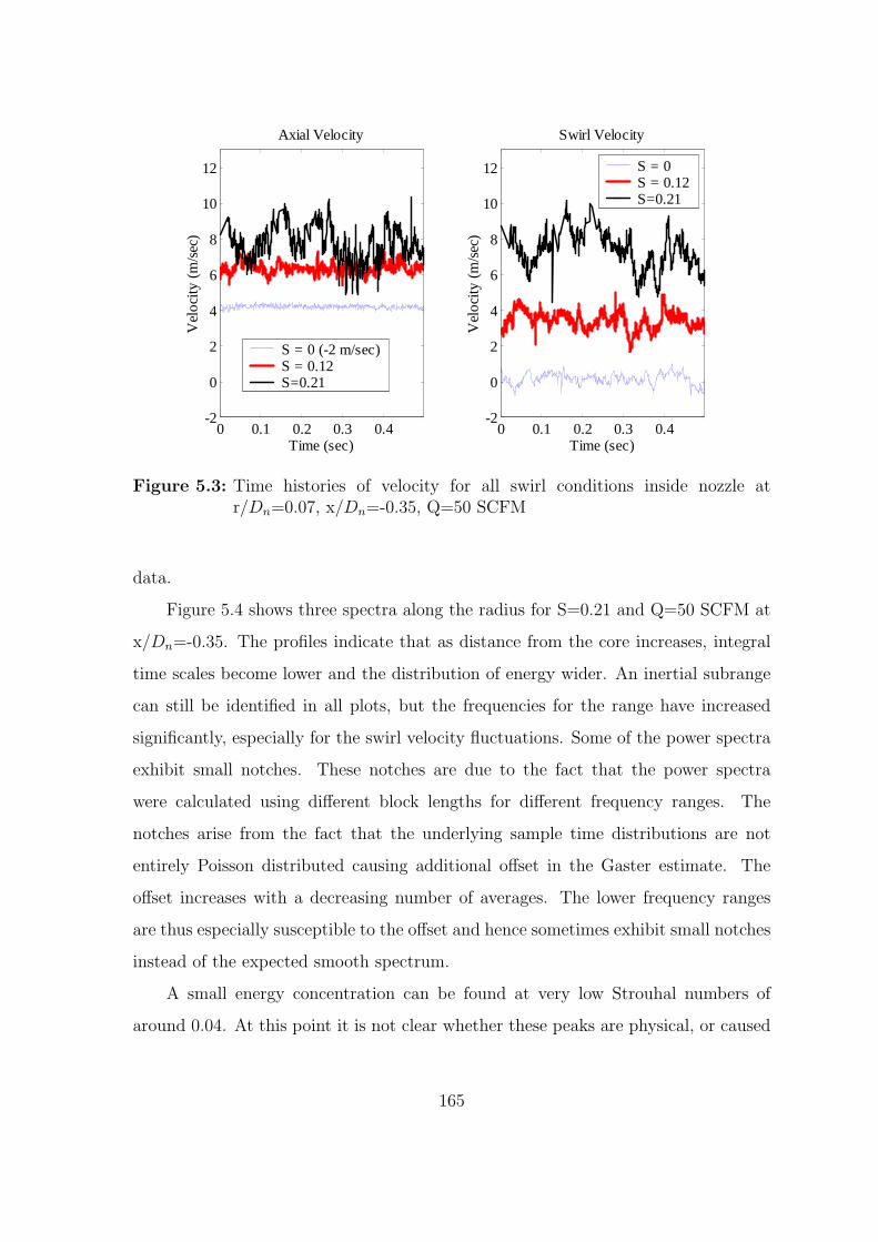
the fluctuations. Figure 5.3 shows the time histories of axial and swirl velocity at the

same conditions as Figure 5.1. The time histories are taken from the beginning of the

middle data block collected. The time histories clearly reflect the large differences in

energy between the different flow conditions. The histories also confirm the relation-

ship between the integral time scales originally deduced from the power spectrum.

The undulations in swirl velocity appear much slower than the undulations in axial

velocity. The time histories do not show any significant periodicity. The 900 Hz peak

seen in the power spectra has too little power to be able to be identified in the time

164

0 0.1 0.2 0.3 0.4-2

0

2

4

6

8

10

12

Axial Velocity

Time (sec)

Vel

oci

ty (

m/s

ec)

S = 0 (-2 m/sec)S = 0.12 S=0.21

0 0.1 0.2 0.3 0.4-2

0

2

4

6

8

10

12

Swirl Velocity

Time (sec)

Vel

oci

ty (

m/s

ec)

S = 0 S = 0.12S=0.21

Figure 5.3: Time histories of velocity for all swirl conditions inside nozzle atr/Dn=0.07, x/Dn=-0.35, Q=50 SCFM

data.

Figure 5.4 shows three spectra along the radius for S=0.21 and Q=50 SCFM at

x/Dn=-0.35. The profiles indicate that as distance from the core increases, integral

time scales become lower and the distribution of energy wider. An inertial subrange

can still be identified in all plots, but the frequencies for the range have increased

significantly, especially for the swirl velocity fluctuations. Some of the power spectra

exhibit small notches. These notches are due to the fact that the power spectra

were calculated using different block lengths for different frequency ranges. The

notches arise from the fact that the underlying sample time distributions are not

entirely Poisson distributed causing additional offset in the Gaster estimate. The

offset increases with a decreasing number of averages. The lower frequency ranges

are thus especially susceptible to the offset and hence sometimes exhibit small notches

instead of the expected smooth spectrum.

A small energy concentration can be found at very low Strouhal numbers of

around 0.04. At this point it is not clear whether these peaks are physical, or caused

165

10-2

10-1

100

101

10-4

10-3

10-2

10-1

100

101 Axial Velocity


No

rmal

ized

po

wer

den

sity

r = 0.07 r = 0.31 r = 0.41 -5/3 slope

10-2

10-1

100

101

10-4

10-3

10-2

10-1

100

101 Swirl Velocity

Strouhal number (f*D/U - f(Hz))N

orm

aliz

ed p

ow

er d

ensi

ty

r = 0.07 r = 0.31 r = 0.41 -5/3 slope

Figure 5.4: Radial comparison of spectra for S=0.21, x/Dn=-0.35, Q=50 SCFM

by variance in the power estimate at low frequency. The peaks are seen in both the

swirl and axial velocities near the core and only in the swirl velocity towards the outer

parts of the flow. The 900 Hz peak also can still be identified in the data although

this becomes more difficult as the inertial subrange extends to higher frequencies.

The fact that the 900 Hz peak is invariant with both flow condition and physical

location in the flow lends further strength to the conclusion that the energy seen at

900 Hz stems from acoustic oscillations that are superposed on the turbulent velocity

fluctuations.

Figure 5.5 shows the power spectra calculated for two different flow rates at

r/Dn=0.07, x/Dn=-0.35 and S=0.12. The flow profile comparisons showed that the

normalized results are not a strong function of flow rate. The results of Figure 5.5

show that this is still the case for the swirl velocity spectrum. The only significant

difference seen here is the fact that as expected, the higher Reynolds number flow has

a smaller integral time scale. Due to the limit in LDV sampling frequency, not the

entire inertial subrange of swirl velocity fluctuations could be resolved for the higher

166

10-2

10-1

100

101

10-4

10-3

10-2

10-1

100

101 Axial Velocity


No

rmal

ized

po

wer

den

sity

Q=50 Q=100 -5/3 slope

10-2

10-1

100

101

10-4

10-3

10-2

10-1

100

101 Swirl Velocity


No

rmal

ized

po

wer

den

sity

Q=50 Q=100 -5/3 slope

Figure 5.5: Comparison of spectra for two flow rates at S=0.12, x/Dn=-0.35

flow-rate. The integral time scale of the axial velocity fluctuations at the higher

flow rate is significantly lower compared to the lower flow rate. Additionally, even

though the frequency scale has been normalized, the extent of energy containing time

scales is significantly extended. At the highest resolved frequency range, the power

spectrum of axial velocity fluctuations at 100 SCFM barely begins to show a linear

slope. The difference in time scales between the axial and swirl velocity fluctuations

was noted earlier but seems to be magnified for the 100 SCFM flow rate. It is clear

that although the time mean statistics at the two flow rates are very similar, the

underlying dynamic state can exhibit significant differences.

Figure 5.6 shows the radial variation of axial and swirl velocity power spectra

for x/Dn=-0.35, S=0.12 and Q=100 SCFM. As was noted for the case of S=0.21,

Q=50 SCFM, the power spectrum of velocity fluctuations extends to higher frequen-

cies outside the vortex core. Correspondingly, the integral time scales of the motions

also decrease. The large disparity observed between the frequency extent of axial and

swirl velocity fluctuations is absent outside the vortex core as well. Axial and swirl

167

10-2

10-1

100

101

10-4

10-3

10-2

10-1

100

101 Axial Velocity


No

rmal

ized

po

wer

den

sity

r = 0.07 r = 0.31 r = 0.41 -5/3 slope

10-2

10-1

100

101

10-4

10-3

10-2

10-1

100

101 Swirl Velocity


orm

aliz

ed p

ow

er d

ensi

ty

r = 0.07 r = 0.31 r = 0.41 -5/3 slope


velocity fluctuations appear to contain energy over nearly the same frequency range.

For the large swirl condition, the disparity was seen to persist outside the vortex core.

Figure 5.6 shows a wide local maximum in the axial velocity power spectrum

around St=3. The energy excess shown around that frequency band is only seen near

the radial location r/Dn=0.31. It is not observed in the swirl velocity spectrum and

is absent in the core of the flow as well as near the wall. Figure 5.7 shows the radial

variation of power spectra under the same conditions except for Q=50 SCFM. The

excess can also be observed here, near the same Strouhal number as for the higher

flow-rate. Similar to the 100 SCFM case, the frequency extent of energy containing

fluctuations does not differ between axial and swirl velocity fluctuations outside of

the vortex core.

Figure 5.8 shows axial variation of the velocity power spectra at r/Dn=0.31,

S=0.12, Q=100 SCFM. Note that the y-axes have been re-scaled to zoom in on the

feature in question. The energy excess observed in the previous two figures is also

seen here as the flow develops. The relative magnitude of the local maximum seems to

168

10-2

10-1

100

101

10-4

10-3

10-2

10-1

100

101 Axial Velocity


No

rmal

ized

po

wer

den

sity

r = 0.07 r = 0.31 r = 0.41 -5/3 slope

10-2

10-1

100

101

10-4

10-3

10-2

10-1

100

101 Swirl Velocity


orm

aliz

ed p

ow

er d

ensi

ty

r = 0.07 r = 0.31 r = 0.41 -5/3 slope


be increasing slightly. More easily identified is the decrease in the integral time scale

of fluctuations as the flow develops downstream. The increase in time scale appears

to be unrelated to the local maximum in axial velocity fluctuations, because the swirl

velocity spectrum exhibits the same trend. The decrease in the integral time scale as

the flow evolves downstream in the nozzle can be understood as the influence of the

growing shear layers at the center and boundary of the flow. As the shear layer grows

the scales of the associated turbulence can also be expected to grow. As the spatial

scales increase, the associated time scales also increase as the predominant velocity

scale remains constant. The question of the origin of the local maximum in the axial

velocity spectrum remains and will be addressed again when the combustor velocity

dynamics are studied.

The power spectra calculated for the nozzle flow field exhibit an interesting range

of behavior in terms of the distribution of the time scales of turbulence. Longer time

scales are observed in the vortex core where the overall fluctuation energy is greatest.

A significant difference between the time scales of axial and swirl velocity fluctuations

169

10-2

10-1

100

101

10-1

100

101 Axial Velocity


No

rmal

ized

po

wer

den

sity

x=-0.35X=-0.69

10-2

10-1

100

101

10-1

100

101 Swirl Velocity


orm

aliz

ed p

ow

er d

ensi

ty

x=-0.35X=-0.69

Figure 5.8: Axial comparison of spectra for S=0.12, r/Dn=0.31, Q=100 SCFM

is found at the core. The difference decreases with increasing radius and decreasing

swirl. The higher integral time scales at the centerline are consistent with the narrower

bandwidth of fluctuations. It is also important to remember that the core exhibits

large shear stresses under swirling conditions. These shear stresses are effective in

redistributing mean momentum.

Using the spectral characteristics it is now possible to postulate how the flow

is able to maintain stability while producing a large amount of turbulent energy. It

is clear from the RMS velocity distributions that the energy produced accumulates

more in the swirl velocity component than in the axial velocity component. Based on

the spectra shown here, the reason for this is that swirl fluctuations are more easily

dissipated. The range of time scales which provide a pipeline to dissipation is much

wider for the swirl velocity. The radial and azimuthal motion of the vortex core allows

the center of the flow to lose energy efficiently to the surrounding fluid via the shear

caused in the azimuthal direction by such motion.

The breakdown of the vortex core can then be associated with the inability

170

of small motions of the core to lose enough turbulent energy. Larger and larger

deflections occur and eventually do not allow the core to recover. This picture explains

why at 100 SCFM, the vortex core breaks down sooner. The increased production of

turbulence at the higher flow rate is confined to the same area. The core movement

can only provide a finite amount of energy dissipation and this level of movement is

reached sooner at the higher flow–rate.

This picture is also consistent with the significant amount of low frequency energy

contained in velocity fluctuations near the vortex core. The low frequency energy

increases with increasing swirl, consistent with the idea that the motion of the core

increases with increasing swirl to provide more effective dissipation of the increased

turbulence production. The idea that a certain limit of turbulent energy can be

contained at the vortex core before the flow becomes unstable and breaks down will

be examined in detail in Chapter 6.

5.2.1.2 Combustor flow dynamics

The dynamics of the flow field downstream of the sudden expansion are expected

to yield an especially rich dynamic picture since the flow field is rapidly evolving

and a lot of turbulent energy is created, transported and dissipated. Similar to the

nozzle flow, it is expected that fluctuation spectra will allow further insight into the

processes responsible for the evolution of the flow field described in Chapter 4.

Figures 5.9 and 5.10 show the radial variation of axial and swirl velocity power

spectra for the condition of zero swirl at x/Dn=0.44 and Q=50 SCFM. Figure 5.9

shows inner radial locations whereas Figure 5.10 shows mostly radial locations out-

side the outer shear layer. The time scales associated with fluctuations in the inner

flow appear to be relatively constant. In the outer shear layer however, at r/Dn=0.66

significantly larger integral time scales are found. Figure 5.10 shows that the entire

outer region of the flow beyond the outer shear layer is dominated by energy distribu-

tions exhibiting a large amount of low frequency energy and large integral time scales

relative to the inner portion of the flow.

The long continuous downward slope of the spectra indicate an efficient transfer

171

10-2

10-1

100

101

10-4

10-3

10-2

10-1

100

101

Axial Velocity


No

rmal

ized

po

wer

den

sity

r = 0.07 r = 0.41 r = 0.66 -5/3 slope

10-2

10-1

100

101

10-4

10-3

10-2

10-1

100

101

Swirl Velocity


orm

aliz

ed p

ow

er d

ensi

ty

r = 0.07 r = 0.41 r = 0.66 -5/3 slope

Figure 5.9: Radial comparison of power spectra for x/Dn=0.44, S=0, Q=50 SCFM(inner flow)

10-2

10-1

100

101

10-4

10-3

10-2

10-1

100

101

Axial Velocity


No

rmal

ized

po

wer

den

sity

r = 0.48 r = 0.83 r = 1.00 -5/3 slope

10-2

10-1

100

101

10-4

10-3

10-2

10-1

100

101

Swirl Velocity


No

rmal

ized

po

wer

den

sity

r = 0.48 r = 0.83 r = 1.00 -5/3 slope

Figure 5.10: Radial comparison of power spectra for x/Dn=0.44, S=0, Q=50 SCFM(outer flow)

172

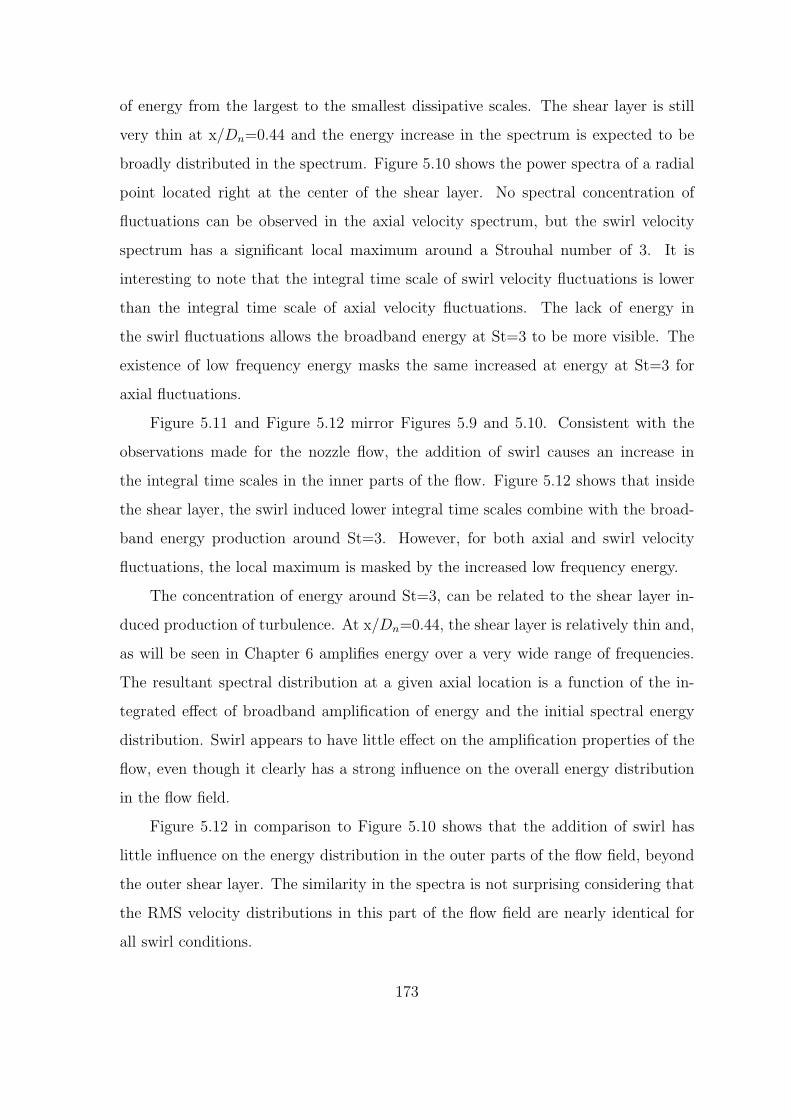
of energy from the largest to the smallest dissipative scales. The shear layer is still

very thin at x/Dn=0.44 and the energy increase in the spectrum is expected to be

broadly distributed in the spectrum. Figure 5.10 shows the power spectra of a radial

point located right at the center of the shear layer. No spectral concentration of

fluctuations can be observed in the axial velocity spectrum, but the swirl velocity

spectrum has a significant local maximum around a Strouhal number of 3. It is

interesting to note that the integral time scale of swirl velocity fluctuations is lower

than the integral time scale of axial velocity fluctuations. The lack of energy in

the swirl fluctuations allows the broadband energy at St=3 to be more visible. The

existence of low frequency energy masks the same increased at energy at St=3 for

axial fluctuations.

Figure 5.11 and Figure 5.12 mirror Figures 5.9 and 5.10. Consistent with the

observations made for the nozzle flow, the addition of swirl causes an increase in

the integral time scales in the inner parts of the flow. Figure 5.12 shows that inside

the shear layer, the swirl induced lower integral time scales combine with the broad-

band energy production around St=3. However, for both axial and swirl velocity

fluctuations, the local maximum is masked by the increased low frequency energy.

The concentration of energy around St=3, can be related to the shear layer in-

duced production of turbulence. At x/Dn=0.44, the shear layer is relatively thin and,

as will be seen in Chapter 6 amplifies energy over a very wide range of frequencies.

The resultant spectral distribution at a given axial location is a function of the in-

tegrated effect of broadband amplification of energy and the initial spectral energy

distribution. Swirl appears to have little effect on the amplification properties of the

flow, even though it clearly has a strong influence on the overall energy distribution

in the flow field.

Figure 5.12 in comparison to Figure 5.10 shows that the addition of swirl has

little influence on the energy distribution in the outer parts of the flow field, beyond

the outer shear layer. The similarity in the spectra is not surprising considering that

the RMS velocity distributions in this part of the flow field are nearly identical for

all swirl conditions.

173

10-2

10-1

100

101

10-4

10-3

10-2

10-1

100

101 Axial Velocity


No

rmal

ized

po

wer

den

sity

r = 0.07 r = 0.41 r = 0.66 -5/3 slope

10-2

10-1

100

101

10-4

10-3

10-2

10-1

100

101 Swirl Velocity


orm

aliz

ed p

ow

er d

ensi

ty

r = 0.07 r = 0.41 r = 0.66 -5/3 slope

Figure 5.11: Radial comparison of power spectra for x/Dn=0.44, S=0.12,Q=50 SCFM (inner flow)

10-2

10-1

100

101

10-4

10-3

10-2

10-1

100

101 Axial Velocity


No

rmal

ized

po

wer

den

sity

r = 0.48 r = 0.83 r = 1.00 -5/3 slope

10-2

10-1

100

101

10-4

10-3

10-2

10-1

100

101 Swirl Velocity


No

rmal

ized

po

wer

den

sity

r = 0.48 r = 0.83 r = 1.00 -5/3 slope

Figure 5.12: Radial comparison of power spectra for x/Dn=0.44, S=0.12,Q=50 SCFM (outer flow)

174

10-2

10-1

100

101

10-4

10-3

10-2

10-1

100

101 Axial Velocity


No

rmal

ized

po

wer

den

sity

r = 0.07 r = 0.41 r = 0.66 -5/3 slope

10-2

10-1

100

101

10-4

10-3

10-2

10-1

100

101 Swirl Velocity


No

rmal

ized

po

wer

den

sity

r = 0.07 r = 0.41 r = 0.66 -5/3 slope


Figure 5.13 shows a comparison of the normalized power spectra of velocity fluc-

tuations at three radial locations in the main part of the flow for x/Dn=0.44, S=0.21

and Q=50 SCFM. Figure 5.14 overlaps Figure 5.13 in radial location and shows the

spectra for points located outside the outer shear layer of the incoming flow. In both

the inner and outer flow, the time scales of swirl and axial velocity fluctuations have

become nearly the same. The significant radial variation of the frequency extent of

the energy containing swirl velocity fluctuations is not observed at x/Dn=0.44. The

spectra of the flow field outside the shear layer resemble those of the swirl velocity

at the centerline of the nozzle. The difference is that here in the recirculation region

of the incoming jet, both swirl and axial velocity fluctuations exhibit the increase in

integral time scale and have an inertial subrange that extends to lower frequencies,

as remarked above.

Figures 5.13 and 5.14 also show several sharper spectral features in the very low

range of Strouhal numbers, below St=0.1. Previous figures exhibit similar features

175

10-2

10-1

100

101

10-4

10-3

10-2

10-1

100

101 Axial Velocity


No

rmal

ized

po

wer

den

sity

r = 0.48 r = 0.83 r = 1.00 -5/3 slope

10-2

10-1

100

101

10-4

10-3

10-2

10-1

100

101 Swirl Velocity


No

rmal

ized

po

wer

den

sity

r = 0.48 r = 0.83 r = 1.00 -5/3 slope


and the discussion that follows also applies to those cases. The time histories of

velocity for several data points are used to examine whether or not these peaks cor-

respond to large scale coherent motion or are merely due to a larger variance in the

spectral estimate at low frequency. Figure 5.15 shows the time history of velocities at

r/Dn=0.41, x/Dn=0.44, S=0.21, Q=50 SCFM. While the axial velocity fluctuations

do not exhibit significant coherent oscillations, the swirl velocity clearly shows sinu-

soidal motion with a frequency of around 4 Hz which corresponds well with the small

spectral peak observed in the spectrum in Figure 5.13 near St=0.05. The oscillations

observed modulate the higher frequency turbulent fluctuations. Towards the end of

the time record, however, the coherence appears to decrease as the oscillations become

blurred. The superimposed turbulence fluctuations remain constant throughout the

record.

A peak at nearly the same frequency is observed in Figure 5.14 in the axial ve-

locity spectrum. A corresponding time record is shown in Figure 5.16. No coherent

176

0 0.5 1 1.54

5

6

7

8Axial Velocity

Time (sec)

Vel

oci

ty (

m/s

ec)

0 0.5 1 1.50

1

2

3

4Swirl Velocity

Time (sec)

Vel

oci

ty (

m/s

ec)

Figure 5.15: Time history of axial and swirl velocity for r/Dn=0.41, x/Dn=0.44,S=0.21, Q=50 SCFM

fluctuations can be distinguished in the time record. This does not imply that co-

herent fluctuations are never present at this point in the flow field. The snap shot

presented in Figure 5.16 just doesn’t show them. Figure 5.15 showed how the fluc-

tuations can lose their coherence gradually. The appearance and disappearance of

coherent fluctuations is not surprising considering the very large amount of energy

in the flow. In the initial times of Figure 5.15, the turbulence seems superimposed

on the wave. This is the picture of instability and turbulence interaction assumed

when a linear stability analysis is performed in turbulent flow. The turbulence and

instability related velocity fluctuations appear independent. However in the latter

parts of the time record the wave becomes smeared and hard to distinguish from the

rest of the turbulence. The smearing and mixing observed can be postulated to be

due to the fact that the turbulence in the flow has significant energy at frequencies

surrounding the oscillation frequency. This energy then overwhelms the energy in

the oscillation and makes it lose coherence. The spectrum at such points will be

similar to the spectra observed here, a small peak at the frequency of instability and

a lot of energy surrounding it. However, short-term coherence may also be due to

the fact that randomly, for short periods of time (on the order of the wavelength

of oscillation) a significant amount of energy accumulates at a certain frequency in

the spectrum. The concentration is not due to instability and therefore eventually

177

0 0.5 1 1.54

5

6

7

8Axial Velocity

Time (sec)

Vel

oci

ty (

m/s

ec)

0 0.5 1 1.50

1

2

3

4Swirl Velocity

Time (sec)

Vel

oci

ty (

m/s

ec)


decays as the energy is again redistributed randomly. The latter explanation is more

plausible because the low frequency peaks are not always observed at same frequency.

Figures 5.17 and 5.18 compare the inner and outer spectral distributions for

S=0.12 at 100 SCFM. As noted for the nozzle, the extent of the energy containing

scales is wider for the higher flow rate. The broadband amplification seen for St=3

at 50 SCFM can still be identified at the same Strouhal number for 100 SCFM.

The underlying spectrum again contains relatively large integral time scales. The

power spectra outside the outer shear layer are very similar to the spectra obtained

at 50 SCFM.

Figure 5.19 shows the radial variation of velocity spectra for x/Dn=0.97, S=0.12,

Q=50 SCFM. The variation shows the influence of the in-tact vortex core as the

integral time scale for the location near the centerline is higher than the integral time

scales for the other locations shown. Away from the centerline the spectra of axial

and swirl velocity are very similar exhibiting a long downward, approximately linear

slope.

The power spectral density of the point r/Dn=0.07 in Figure 5.19 once again

contains a small concentration of spectral energy near a Strouhal number of 0.05.

The experimental conditions are different here though with S=0.12 instead of 0.21.

Figure 5.20 shows a time snapshot of the velocity field at this location. Similar to

178

10-2

10-1

100

101

10-4

10-3

10-2

10-1

100

101 Axial Velocity


No

rmal

ized

po

wer

den

sity

r = 0.07 r = 0.41 r = 0.66 -5/3 slope

10-2

10-1

100

101

10-4

10-3

10-2

10-1

100

101 Swirl Velocity


orm

aliz

ed p

ow

er d

ensi

ty

r = 0.07 r = 0.41 r = 0.66 -5/3 slope


10-2

10-1

100

101

10-3

10-2

10-1

100

101

Axial Velocity


No

rmal

ized

po

wer

den

sity

r = 0.48 r = 0.83 r = 1.00 -5/3 slope

10-2

10-1

100

101

10-3

10-2

10-1

100

101

Swirl Velocity


No

rmal

ized

po

wer

den

sity

r = 0.48 r = 0.83 r = 1.00 -5/3 slope


179

10-2

10-1

100

101

10-4

10-3

10-2

10-1

100

101 Axial Velocity


No

rmal

ized

po

wer

den

sity

r = 0.07 r = 0.41 r = 0.66 -5/3 slope

10-2

10-1

100

101

10-4

10-3

10-2

10-1

100

101 Swirl Velocity


orm

aliz

ed p

ow

er d

ensi

ty

r = 0.07 r = 0.41 r = 0.66 -5/3 slope

Figure 5.19: Radial comparison of spectra for x/Dn=0.97, S=0.12, Q=50 SCFM

Figure 5.15, the axial velocity does not exhibit coherent fluctuations. However, large

coherent fluctuations are observed in the swirl velocity. Still, the periodicity of the

fluctuations in Figure 5.20 appears to be somewhat blurred by the superimposed

turbulence, as was seen in Figure 5.15.

Whether or not these low frequency coherent motions actually correspond to true

flow instabilities must be put in question with their apparently near random occur-

rence. However, the behavior clearly shows that in strongly turbulent flows, shear

layer instabilities will be difficult to excite because of an abundance of energy sur-

rounding the excitation frequency. In order for excitation to produce highly coherent

structures, the excitation must match or exceed the energy of the turbulent fluctua-

tions which is difficult to accomplish in the present setup. Once such high excitation

is achieved, the results may not at all correspond to linear behavior. These issues may

also have influenced the success of Panda and McLaughlin (1994) in their attempt

to excite swirling flow. In this view sharp spectral peaks cannot be expected. Broad

peaks can develop when a certain band of frequencies is consistently amplified as a

flow evolves downstream. However, this situation is clearly limited to cases where the

180

0 0.2 0.44

5

6

7

8Axial Velocity

Time (sec)

Vel

oci

ty (

m/s

ec)

0 0.2 0.40

1

2

3

4Swirl Velocity

Time (sec)

Vel

oci

ty (

m/s

ec)


flow is developing relatively slowly so that the range of amplified frequencies exhibits

significant overlap along the development path of the flow.

Figure 5.21 shows the radial variation of power spectra for S=0.21, 50 SCFM

at x/Dn=0.97. The radial variation of the integral time scale is lost at this station.

All radial locations have nearly the same integral time scale and spectral shape. The

outer radial locations appear to have a slightly more linear distribution of energy in

the spectrum indicating more efficient transfer to small scales. The location closest to

the centerline exhibits decreasing energy for low Strouhal numbers (less than 0.4) and

for Strouhal numbers above 5. In the intermediate range the slope in the spectrum is

flatter possibly indicating turbulence generation. The flatter intermediate distribution

is seen in both the axial and swirl velocity spectra. The range of Strouhal numbers

in question is often associated with fluid dynamic instabilities, further supporting the

claim that turbulence generation is interrupting the constant flow of energy to smaller

scales.

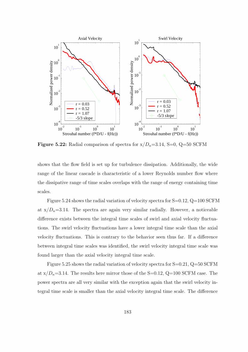
Figure 5.22 shows the radial variation of velocity spectra for the S=0, Q=50 SCFM

case at x/Dn=3.14. The jet is at this point near the end of its initial development

stage, with the potential core still visible. The axial velocity fluctuations exhibit a

wide and significant concentration of spectral energy around a Strouhal number of

0.4. The swirl velocity spectrum also shows traces of added energy around St=0.4.

This type of broadband peak can be expected in a slowly developing jet type flow,

181

10-2

10-1

100

101

10-4

10-3

10-2

10-1

100

101 Axial Velocity


No

rmal

ized

po

wer

den

sity

r = 0.07 r = 0.41 r = 0.66 -5/3 slope

10-2

10-1

100

101

10-4

10-3

10-2

10-1

100

101 Swirl Velocity


orm

aliz

ed p

ow

er d

ensi

ty

r = 0.07 r = 0.41 r = 0.66 -5/3 slope


that has significant inlet turbulence. The peak Strouhal number of 0.4 is in the range

of frequencies commonly encountered for free jet shear flows (e.g. Wygnanski and

Petersen, 1987). The instability found at this axial station is seen to develop starting

from x/Dn=0.97. The instability development will be studied in detail in Section 5.3.

Figure 5.23 compares spectra for various radial locations in the flow for the

S=0.12, Q=50 SCFM case at x/Dn=3.14. The spectra are all extremely similar. In

Chapter 4 it was noted how quickly the free vortex cases with swirl develop down-

stream relative to the zero swirl case. The flow at this axial station has very high

RMS velocity. The RMS velocity is distributed relatively evenly compared to the

earlier stages of development of the flow. The radial variation in velocity spectra

bears this out. All the spectra exhibit a nearly linear (on the log-log plot) decline

over the entire range of Strouhal numbers able to be measured. The linear decline

covers more than three decades of energy content. The slope of the line is near -5/3

but slightly shallower in some ranges of Strouhal number consistent with some con-

tinued broadband turbulence production. Overall, the long linear cascade of energy

182

10-2

10-1

100

101

10-4

10-3

10-2

10-1

100

101

Axial Velocity


No

rmal

ized

po

wer

den

sity

r = 0.03 r = 0.52 r = 1.07 -5/3 slope

10-2

10-1

100

101

10-4

10-3

10-2

10-1

100

101 Swirl Velocity


orm

aliz

ed p

ow

er d

ensi

ty

r = 0.03 r = 0.52 r = 1.07 -5/3 slope

Figure 5.22: Radial comparison of spectra for x/Dn=3.14, S=0, Q=50 SCFM

shows that the flow field is set up for turbulence dissipation. Additionally, the wide

range of the linear cascade is characteristic of a lower Reynolds number flow where

the dissipative range of time scales overlaps with the range of energy containing time

scales.

Figure 5.24 shows the radial variation of velocity spectra for S=0.12, Q=100 SCFM

at x/Dn=3.14. The spectra are again very similar radially. However, a noticeable

difference exists between the integral time scales of swirl and axial velocity fluctua-

tions. The swirl velocity fluctuations have a lower integral time scale than the axial

velocity fluctuations. This is contrary to the behavior seen thus far. If a difference

between integral time scales was identified, the swirl velocity integral time scale was

found larger than the axial velocity integral time scale.

Figure 5.25 shows the radial variation of velocity spectra for S=0.21, Q=50 SCFM

at x/Dn=3.14. The results here mirror those of the S=0.12, Q=100 SCFM case. The

power spectra are all very similar with the exception again that the swirl velocity in-

tegral time scale is smaller than the axial velocity integral time scale. The difference

183

10-2

10-1

100

101

10-4

10-3

10-2

10-1

100

101

Axial Velocity


No

rmal

ized

po

wer

den

sity

r = 0.03 r = 0.52 r = 1.07 -5/3 slope

10-2

10-1

100

101

10-4

10-3

10-2

10-1

100

101

Swirl Velocity


No

rmal

ized

po

wer

den

sity

r = 0.03 r = 0.52 r = 1.07 -5/3 slope


10-2

10-1

100

101

10-4

10-3

10-2

10-1

100

101

Axial Velocity


No

rmal

ized

po

wer

den

sity

r = 0.03 r = 0.52 r = 1.07 -5/3 slope

10-2

10-1

100

101

10-4

10-3

10-2

10-1

100

101

Swirl Velocity


No

rmal

ized

po

wer

den

sity

r = 0.03 r = 0.52 r = 1.07 -5/3 slope


184

10-2

10-1

100

101

10-4

10-3

10-2

10-1

100

101 Axial Velocity


No

rmal

ized

po

wer

den

sity

r = 0 r = 0.55 r = 1.10 -5/3 slope

10-2

10-1

100

101

10-4

10-3

10-2

10-1

100

101 Swirl Velocity


orm

aliz

ed p

ow

er d

ensi

ty

r = 0 r = 0.55 r = 1.10 -5/3 slope


between time scales seen here appears smaller than for the S=0.12, Q=100 SCFM

case. The S=0.21 case develops the quickest of all the free vortex geometry flows

studied. It is therefore possible that the integral time scales of swirl velocity fluctua-

tions have decreased because the energy in the low Strouhal number range has begun

to be dissipated. The dissipated energy is not replaced because no significant shear

remains in the flow field to produce turbulent energy. The dissipation of axial velocity

fluctuations is relatively slower because the axial velocity fluctuations, relative to the

axial mean flow are weaker than the swirl velocity fluctuations relative to the swirl

mean flow. Since dissipation scales with the cube of the strength of these oscillations,

the view that dissipation is more rapid for swirl velocity oscillations is not untenable.

These observations rely on the idea that to some extent the velocity fluctuations

and the energy contained in them can be considered independent for each component

of velocity. This is of course not entirely true but some degree of separation exists

and intuitively the results presented can for the most part be explained using the

ideas relying on independence.

185

5.2.2 Annulus geometry

The results presented for the annulus geometry use the same normalization pro-

cedure as for the free vortex geometry. The reference length however, as in Chapter 4

is taken to be the hydraulic diameter of the annulus which is equal to 1.9 in. The

reference velocities are the area mean values calculated inside the nozzle for each case.

The values are given in Table 4.1.

5.2.2.1 Nozzle flow dynamics

Figure 5.26 shows velocity spectra for all swirl levels studied at x/Dh=-0.52,

r/Dh=0.42. The radial location chosen is relatively close to the center–body. The

spectra for S=0.60 exhibit large spectral peaks that are uncommonly narrow. These

peaks are part of a larger instability in the downstream flow field. The instability will

be discussed in detail below in Section 5.3. The integral time scale for the S=0.60

case is dominated by the instability time scale and thus much lower than that of the

other two cases studied. Consistent with results seen in the free vortex geometry the

integral time scale of the S=0.28 flow field is greater than that of the S=0 flow field.

Similarly again, the axial velocity integral time scale is smaller than the swirl velocity

integral time scale. For both the S=0.60, instability influenced spectra and the S=0

spectra, there are no noticeable differences in integral time scale between swirl and

axial velocity. The -5/3 portions of the spectra line up very closely for all cases.

Contrary to the free vortex geometry results, the swirl and axial velocity fluctuations

exhibit the inertial subrange in the same range of Strouhal numbers.

Figure 5.27 shows the radial variation of spectra for the S=0, Q=50 SCFM case.

Only small differences exist between the radial locations compared. A slight trend

towards longer integral time scales with increasing radius may be extracted from the

swirl velocity spectra. The axial velocity spectra do not exhibit the same trend. Note

that the 900 Hz spectral peak found consistently in the nozzle and combustor is absent

here. The absence of the peak may be due to the fact that it is masked by somewhat

broader band turbulent fluctuations in the annulus geometry case. However, another

186

10-2

10-1

100

101

10-4

10-3

10-2

10-1

100

101 Axial Velocity


No

rmal

ized

po

wer

den

sity

S = 0 S = 0.28 S=0.60 -5/3 slope

10-2

10-1

100

101

10-4

10-3

10-2

10-1

100

101 Swirl Velocity


orm

aliz

ed p

ow

er d

ensi

ty

S = 0 S = 0.28 S=0.60 -5/3 slope

Figure 5.26: Comparison of power spectra for all swirl levels for r/Dh=0.42, x/Dh=-0.53, Q=50 SCFM

reason for the absence of the peak is that the first azimuthal mode of the downstream

section cannot be admitted into the nozzle due to the presence of the center–body.

Figure 5.28 shows the radial variation of spectra for the S=0.28, Q=50 SCFM

case. As already noted for Figure 5.26, the integral time scale of swirl velocity fluc-

tuations increases with the addition of swirl. The integral time scale of axial velocity

fluctuations is again found insensitive to the addition of swirl and no radial depen-

dence of the axial velocity integral time scale can be detected. A bulge in the energy

spectrum is detected around St=3, similar to the S=0.12 case for the free vortex ge-

ometry. Figure 5.28 shows that near the center–body, similar to the free vortex case,

the swirl velocity fluctuations exhibit a narrower bandwidth. The outer two radial

locations do not exhibit any differences in bandwidth compared to the axial velocity

fluctuations.

Figure 5.29 presents the results for the radial variation of spectra at S=0.6,

Q=50 SCFM, x/Dh=-0.53. The spectral peak identified in Figure 5.26 can be identi-

fied in all the spectra shown. Since these spectra are normalized by the local RMS ve-

187

10-2

10-1

100

101

10-4

10-3

10-2

10-1

100

101 Axial Velocity


No

rmal

ized

po

wer

den

sity

r = 0.39 r = 0.55 r = 0.68 -5/3 slope

10-2

10-1

100

101

10-4

10-3

10-2

10-1

100

101 Swirl Velocity


No

rmal

ized

po

wer

den

sity

r = 0.39 r = 0.55 r = 0.68 -5/3 slope

Figure 5.27: Radial comparison of spectra for x/Dh=-0.53, S=0, Q=50 SCFM

10-2

10-1

100

101

10-4

10-3

10-2

10-1

100

101 Axial Velocity


No

rmal

ized

po

wer

den

sity

r = 0.39 r = 0.55 r = 0.68 -5/3 slope

10-2

10-1

100

101

10-4

10-3

10-2

10-1

100

101 Swirl Velocity


No

rmal

ized

po

wer

den

sity

r = 0.39 r = 0.55 r = 0.68 -5/3 slope

Figure 5.28: Radial comparison of spectra for x/Dh=-0.53, S=0.28, Q=50 SCFM

188

10-2

10-1

100

101

10-4

10-3

10-2

10-1

100

101 Axial Velocity


No

rmal

ized

po

wer

den

sity

r = 0.39 r = 0.55 r = 0.68 -5/3 slope

10-2

10-1

100

101

10-4

10-3

10-2

10-1

100

101 Swirl Velocity


orm

aliz

ed p

ow

er d

ensi

ty

r = 0.39 r = 0.55 r = 0.68 -5/3 slope

Figure 5.29: Radial comparison of spectra for x/Dh=-0.53, S=0.60, Q=50 SCFM

locity it is difficult to determine from the figure whether the oscillations are strongest

in the inner or outer parts of the flow (see Section 5.3). Note that some of the spectra

are cut off at relatively low Strouhal number. The reason for the cutoff is due to the

difficulty of obtaining high data rates under these conditions.

Figure 5.30 compares velocity spectra at the two measured axial locations (x/Dh=-

0.53,x/Dh=-1.06) for r/Dh=0.50 at S=0, Q=50 SCFM. Figure 5.31 is the analog of

Figure 5.30, except for S=0.28. Both figures show clearly that little evolution takes

place in the spectrum between the two axial locations at the presented radial loca-

tion. Since the chosen radial location is in the middle of the annulus, no differences

between the S=0 and S=0.28 integral time scales can be detected. The integral time

scales of axial and swirl velocity fluctuations are also nearly the same.

Figure 5.32 shows the axial evolution of velocity spectra for the S=0.60, Q=50 SCFM

case at r/Dh=0.50. The instability observed at x/Dh=-0.53, can still be observed in

the upstream spectra although their strength appears to be reduced significantly.

Apart from the lower instability intensity the remainder of the spectrum appears to

189

10-2

10-1

100

101

10-4

10-3

10-2

10-1

100

101 Axial Velocity


No

rmal

ized

po

wer

den

sity

x=-0.53 X=-1.06 -5/3 slope

10-2

10-1

100

101

10-4

10-3

10-2

10-1

100

101 Swirl Velocity


No

rmal

ized

po

wer

den

sity

x=-0.53 X=-1.06 -5/3 slope

Figure 5.30: Axial comparison of power spectra for r/Dh=0.50, S=0, Q=50 SCFM

10-2

10-1

100

101

10-4

10-3

10-2

10-1

100

101 Axial Velocity


No

rmal

ized

po

wer

den

sity

x=-0.53 x=-1.06 -5/3 slope

10-2

10-1

100

101

10-4

10-3

10-2

10-1

100

101 Swirl Velocity


No

rmal

ized

po

wer

den

sity

x=-0.53 x=-1.06 -5/3 slope

Figure 5.31: Axial comparison of spectra for r/Dh=0.50, S=0.28, Q=50 SCFM

190

10-2

10-1

100

101

10-4

10-3

10-2

10-1

100

101 Axial Velocity


No

rmal

ized

po

wer

den

sity

x=-0.53 x=-1.06 -5/3 slope

10-2

10-1

100

101

10-4

10-3

10-2

10-1

100

101 Swirl Velocity


orm

aliz

ed p

ow

er d

ensi

ty

x=-0.53 x=-1.06 -5/3 slope

Figure 5.32: Axial comparison of power spectra for r/Dh=0.50, S=0, Q=50 SCFM

be maintain constant shape as the flow evolves downstream.

Figure 5.33 compares the spectra for both flow rates at r/Dh=0.50, x/Dh=-0.53

and S=0. The plot shows that the spectrum is a very weak function of flow rate. The

similarity observed in Figure 5.33 is not surprising considering the strong similarity

in mean and RMS velocity profiles observed in Chapter 4.

Figure 5.34 compares the spectra from both flow rates at r/Dh=0.50, x/Dh=-

1.06 and S=0.28. Similar to Figure 5.33, no significant change in the shape of the

spectra is observed when flow rate is increased. Figure 5.36 does exhibit an offset

between the two curves that was not observed for the S=0 case. The offset would

seem to indicate a relative decrease in the integral time scale of fluctuations. A linear

decrease in the integral time scale is accounted for by the normalization of the power

spectrum by the Strouhal number as discussed in Section 5.1. The decrease exhibited

by Figure 5.34 thus suggests a steeper decrease in time scale. The difference observed

here for the two flow rates is consistent with the differences observed in the RMS

velocity profiles shown in Chapter 4, Figure 4.43. In the inner and middle parts of

191

10-2

10-1

100

101

10-4

10-3

10-2

10-1

100

101 Axial Velocity


No

rmal

ized

po

wer

den

sity

Q = 50 Q = 100 -5/3 slope

10-2

10-1

100

101

10-4

10-3

10-2

10-1

100

101 Swirl Velocity


orm

aliz

ed p

ow

er d

ensi

ty

Q = 50 Q = 100 -5/3 slope

Figure 5.33: Comparison of power spectra from both flow rates at r/Dh=0.50,x/Dh=-0.53, S=0

the flow, the higher flow rate exhibits higher normalized RMS velocities. The higher

RMS velocities will lead to a lower normalized integral time scale. In the outer parts

of the annulus, the normalized RMS velocity profiles for the two flow rates overlap

again and a plot of the velocity spectra here confirms this, Figure 5.35. Figure 5.35

also shows that the bulge in energy around St=3 observed for 50 SCFM can also be

identified in the spectra of the higher flow rate case.

Figure 5.36 compared the spectra at both flow rates for r/Dh=0.50, x/Dh=-0.53

and S=0.60. The spectra show that the instability observed at 50 SCFM can also be

identified at the same Strouhal number at 100 SCFM. An even larger percentage of

the total energy seems to be contained in the instability related fluctuations at the

higher flow rate. Overall the two spectra are remarkably similar as expected given

the high degree of similarity also seen for the S=0.60 case in Chapter 4.

192

10-2

10-1

100

101

10-4

10-3

10-2

10-1

100

101 Axial Velocity


No

rmal

ized

po

wer

den

sity

Q = 50 Q = 100 -5/3 slope

10-2

10-1

100

101

10-4

10-3

10-2

10-1

100

101 Swirl Velocity


orm

aliz

ed p

ow

er d

ensi

ty

Q = 50 Q = 100 -5/3 slope

Figure 5.34: Comparison of power spectra from both flow rates at r/Dh=0.50,x/Dh=-0.53, S=0.28

10-2

10-1

100

101

10-4

10-3

10-2

10-1

100

101 Axial Velocity


No

rmal

ized

po

wer

den

sity

Q = 50 Q = 100 -5/3 slope

10-2

10-1

100

101

10-4

10-3

10-2

10-1

100

101 Swirl Velocity


No

rmal

ized

po

wer

den

sity

Q = 50 Q = 100 -5/3 slope


193

10-2

10-1

100

101

10-4

10-3

10-2

10-1

100

101 Axial Velocity


No

rmal

ized

po

wer

den

sity

Q = 50 Q = 100 -5/3 slope

10-2

10-1

100

101

10-4

10-3

10-2

10-1

100

101 Swirl Velocity


No

rmal

ized

po

wer

den

sity

Q = 50 Q = 100 -5/3 slope


194

5.2.2.2 Combustor flow dynamics

Figures 5.37 and 5.38 show the radial variation of the velocity spectra at x/Dh=0.68

for S=0, Q=50 SCFM in the inner and outer part of the flow field respectively. The

spectra in the inner part of the flow field, including the spectra immediately behind

the center–body are all very similar. In the outer shear layer (r/Dh=0.66, r/Dh=0.76),

the swirl velocity spectrum exhibits a bulge of energy near St=3 as observed previ-

ously for several experimental conditions. The integral time scales do not differ for

swirl or axial velocity fluctuations in any part of the flow field. However, both axial

and swirl velocity fluctuations increase in integral time scale abruptly outside the

outer shear layer (r/Dh=1.18, r/Dh=1.50). A linear slope is found throughout the

range of Strouhal numbers captured. The long linear cascade of energy indicates a

very dissipative flow where dissipation occurs over a wide range of scales. The en-

ergy source for this area of the flow is not the local flow but rather the outer shear

layer. The outer recirculation zone represents the necessary means of transport for

the energy.

Figures 5.38 also shows the return of the high frequency peak in the spectrum.

The frequency appears shifted towards lower Strouhal numbers, which is consistent

with the different normalization used for the annulus geometry. The underlying fre-

quency has not changed. This shows that the downstream duct acoustics have not

changed significantly with the addition of the center–body. The center of the flow

field does not show the high frequency acoustic peak in most plots because the ve-

locity fluctuation energy is high enough to mask the acoustic peak. In the nozzle the

RMS velocities are much lower in most cases and the absence of the high frequency

peak in these cases can be associated with the fact that the first azimuthal mode is

not admitted into the nozzle with the center–body present (see Section 5.2.1.1).

Figures 5.39 and 5.40 show the radial variation of power spectra at x/Dh=0.68

for S=0.28, Q=50 SCFM. Except, behind the center–body the spectra for the entire

radial extent of the flow field at x/Dh=0.68 are very similar. The large difference

in time scales observed for the S=0 case across the outer shear layer is not observed

195

10-2

10-1

100

101

10-4

10-3

10-2

10-1

100

101 Axial Velocity


No

rmal

ized

po

wer

den

sity

r = 0.03 r = 0.34 r = 0.76 -5/3 slope

10-2

10-1

100

101

10-4

10-3

10-2

10-1

100

101 Swirl Velocity


orm

aliz

ed p

ow

er d

ensi

ty

r = 0.03 r = 0.34 r = 0.76 -5/3 slope

Figure 5.37: Radial comparison of power spectra at x/Dh=0.68 for S=0,Q=50 SCFM (inner flow field)

10-2

10-1

100

101

10-4

10-3

10-2

10-1

100

101

Axial Velocity


No

rmal

ized

po

wer

den

sity

r = 0.66 r = 1.18 r = 1.50 -5/3 slope

10-2

10-1

100

101

10-4

10-3

10-2

10-1

100

101

Swirl Velocity


No

rmal

ized

po

wer

den

sity

r = 0.66 r = 1.18 r = 1.50 -5/3 slope

Figure 5.38: Radial comparison of power spectra at x/Dh=0.68 for S=0,Q=50 SCFM (outer flow field)

196

10-2

10-1

100

101

10-4

10-3

10-2

10-1

100

101 Axial Velocity


No

rmal

ized

po

wer

den

sity

r = 0.03 r = 0.34 r = 0.76 -5/3 slope

10-2

10-1

100

101

10-4

10-3

10-2

10-1

100

101 Swirl Velocity


orm

aliz

ed p

ow

er d

ensi

ty

r = 0.03 r = 0.34 r = 0.76 -5/3 slope

Figure 5.39: Radial comparison of power spectra at x/Dh=0.68 for S=0.28,Q=50 SCFM (inner flow field)

here. The fact that the spectra beyond the outer shear layer remain similar to the

spectra of the inner flow can be related to the fact that although the axial velocity has

decreased significantly in the outer shear layer, significant swirl velocity remains. The

presence of swirl introduces shear into the flow which causes turbulence production

in this area of the flow field. It should also be noted that the outer shear layer spectra

contain a small bulge in energy as observed previously in several flow fields around

St=3.

The spectrum of swirl velocities has a small local maximum around St=0.8. The

peak is not observed for the axial velocity fluctuations but this is not surprising,

considering that axial RMS velocity fluctuations have a local minimum in the center

of the flow field. The Strouhal number of St=0.8 can be related to a Strouhal number

of 0.42 based on the center–body diameter. This Strouhal number is in the range

where vortex shedding is frequently observed. The development of the wake dynamics

will be followed downstream (see Figure 5.43).

Figures 5.41 and 5.42 show the radial variation of velocity power spectra for

197

10-2

10-1

100

101

10-4

10-3

10-2

10-1

100

101 Axial Velocity


No

rmal

ized

po

wer

den

sity

r = 0.66 r = 1.18 r = 1.50 -5/3 slope

10-2

10-1

100

101

10-4

10-3

10-2

10-1

100

101 Swirl Velocity


orm

aliz

ed p

ow

er d

ensi

ty

r = 0.66 r = 1.18 r = 1.50 -5/3 slope

Figure 5.40: Radial comparison of power spectra at x/Dh=0.68 for S=0.28,Q=50 SCFM (outer flow field)

x/Dh=0.68, S=0.60 and Q=50 SCFM. The inner flow power spectra are dominated

by the large instability observed also in the nozzle. The strength of the oscillations

appears to be greater at this axial location than in the nozzle. Beyond the outer shear

layer however, evidence of the instability disappears quickly from the spectra. It is

interesting to note that the axial velocity spectrum immediately behind the nozzle

shows almost no trace of the instability, while the instability oscillations in the swirl

velocity are very strong. For S=0.29, similar behavior was observed. See Section 5.3

for a comprehensive analysis of the instability.

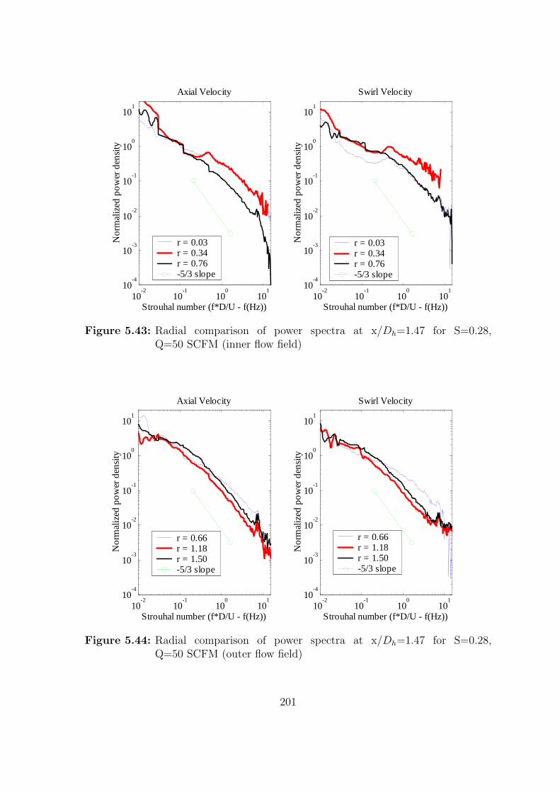
Figures 5.43 and 5.44 show radial variation of velocity spectra for x/Dh=1.47,

S=0.28, Q=50 SCFM. The inner and outer parts of the flow are starting to look very

similar. Both inner and outer flows exhibit a large amount of low frequency energy.

In the center of flow, some leveling out of the spectra indicates continued turbulence

production. Near St=0.4 some concentration of spectral energy can be observed for

r less than 0.5. Figure 4.51 of Chapter 4 shows that the axial velocity peaks at

r/Dh=0.5. The spectral peak is thus due to inner shear layer dynamics. The spectral

198

10-2

10-1

100

101

10-4

10-3

10-2

10-1

100

101 Axial Velocity


No

rmal

ized

po

wer

den

sity

r = 0.03 r = 0.34 r = 0.76 -5/3 slope

10-2

10-1

100

101

10-4

10-3

10-2

10-1

100

101 Swirl Velocity


orm

aliz

ed p

ow

er d

ensi

ty

r = 0.03 r = 0.34 r = 0.76 -5/3 slope


10-2

10-1

100

101

10-4

10-3

10-2

10-1

100

101 Axial Velocity


No

rmal

ized

po

wer

den

sity

r = 0.66 r = 1.18 r = 1.50 -5/3 slope

10-2

10-1

100

101

10-4

10-3

10-2

10-1

100

101 Swirl Velocity


No

rmal

ized

po

wer

den

sity

r = 0.66 r = 1.18 r = 1.50 -5/3 slope


199

peak observed in the center of the flow field for x/Dh=0.68, was observed at St=0.8.

The approximate 2 to 1 relationship between the frequency peak at x/Dh=0.68

and x/Dh=1.47 can be seen as evidence for vortex merging, although the frequency

peak is relatively weak. An alternative view has to do with the evolving linear sta-

bility characteristics of the flow field. At the base of the shear layer, a wide range

of Strouhal numbers is amplified. As the flow evolves downstream, the shear layer

grows and the band of amplified frequencies decreases and shifts downward in fre-

quency. At each axial station, a spectral peak is seen at the frequency that has the

highest integrated energy growth over the entire range of flow development to that

point. As the shear layer thickens, the amplification rates decrease, the bandwidth of

amplified Strouhal numbers decreases and the range of amplified Strouhal numbers

shifts to lower Strouhal numbers. Chapter 6 will examine the stability of the wake

flow behind the center–body. For very rapid shear layer development, the spectral

energy amplification may be so smeared that it is difficult to distinguish from random,

turbulence induced energy production. The dynamics observed here will be discussed

in greater detail in Section 5.3.3.

Figures 5.45 and 5.46 show the radial variation of velocity spectra for x/Dh=1.47,

S=0.29 and Q=100 SCFM. The spectra are in general very similar to the lower flow

rate spectra. Several differences are however worth pointing out. The spectral peaks

around St=0.4 are stronger here and the peak frequency seems to drift somewhat

with radial location. Another feature is the extremely large amount of low frequency

energy, especially at r/Dh=0.34. The y-scale of the plot had to be expanded sig-

nificantly to capture the amount of energy. The y-intercept is proportional to the

integral time scale. The cause for the very high low frequency energy is a type of

intermittency that was found in this flow field at both the lower and higher flow rates.

The associated structures and further details are described in Section 5.3.3.

Figures 5.47 and 5.48 show the radial variation of spectra for x/Dh=1.47, S=0.60

and Q=50 SCFM. The instability observed upstream is still visible here although in

much weaker form. The instability is strongest in the axial velocity fluctuations and

can barely be distinguished in the swirl velocity spectra. Evidence of the instability

200

10-2

10-1

100

101

10-4

10-3

10-2

10-1

100

101

Axial Velocity


No

rmal

ized

po

wer

den

sity

r = 0.03 r = 0.34 r = 0.76 -5/3 slope

10-2

10-1

100

101

10-4

10-3

10-2

10-1

100

101

Swirl Velocity


orm

aliz

ed p

ow

er d

ensi

ty

r = 0.03 r = 0.34 r = 0.76 -5/3 slope


10-2

10-1

100

101

10-4

10-3

10-2

10-1

100

101

Axial Velocity


No

rmal

ized

po

wer

den

sity

r = 0.66 r = 1.18 r = 1.50 -5/3 slope

10-2

10-1

100

101

10-4

10-3

10-2

10-1

100

101

Swirl Velocity


No

rmal

ized

po

wer

den

sity

r = 0.66 r = 1.18 r = 1.50 -5/3 slope


201

10-2

10-1

100

10-4

10-3

10-2

10-1

100

101

102 Axial Velocity


No

rmal

ized

po

wer

den

sity

r = 0.03 r = 0.34 r = 0.76 -5/3 slope

10-2

10-1

100

10-4

10-3

10-2

10-1

100

101

102 Swirl Velocity


orm

aliz

ed p

ow

er d

ensi

ty

r = 0.03 r = 0.34 r = 0.76 -5/3 slope


10-2

10-1

100

10-4

10-3

10-2

10-1

100

101

Axial Velocity


No

rmal

ized

po

wer

den

sity

r = 0.66 r = 1.13 r = 1.45 -5/3 slope

10-2

10-1

100

10-4

10-3

10-2

10-1

100

101

Swirl Velocity


No

rmal

ized

po

wer

den

sity

r = 0.66 r = 1.13 r = 1.45 -5/3 slope


202

10-2

10-1

100

101

10-4

10-3

10-2

10-1

100

101 Axial Velocity


No

rmal

ized

po

wer

den

sity

r = 0.03 r = 0.34 r = 0.76 -5/3 slope

10-2

10-1

100

101

10-4

10-3

10-2

10-1

100

101 Swirl Velocity


orm

aliz

ed p

ow

er d

ensi

ty

r = 0.03 r = 0.34 r = 0.76 -5/3 slope


can no longer be seen at the center of the flow. Overall the spectra are very similar

and especially compared with the S=0.28(0.29) case, a relatively small amount of low

frequency energy is present in the flow.

Figures 5.49 and 5.50 show the results for the same swirl number and axial loca-

tion as Figures 5.47 and 5.48 except at the higher flow rate of 100 SCFM. The traces

of the instability are stronger at the higher flow rate, and can be easily distinguished

in both the axial and swirl velocity spectra. Similar to the lower flow rate, evidence of

the instability is weakest at the very center of the flow and in the outermost areas of

the flow field. Swirl velocity fluctuation integral timescales are a decreasing function

of radius in the inner portion of the flow field. The trend may also be related to the

presence of the instability just outside the inner core of the flow field.

Figure 5.51 shows the power spectra of velocity at three radial locations for

x/Dh=4.79, S=0 and Q=50 SCFM. Both axial and swirl velocity spectra exhibit a

small local maximum in energy near St=0.3, likely due to the developing jet and

associated shear layer. In the outer part of the flow field, large scales contain a

203

10-2

10-1

100

101

10-4

10-3

10-2

10-1

100

101 Axial Velocity


No

rmal

ized

po

wer

den

sity

r = 0.66 r = 1.18 r = 1.50 -5/3 slope

10-2

10-1

100

101

10-4

10-3

10-2

10-1

100

101 Swirl Velocity


orm

aliz

ed p

ow

er d

ensi

ty

r = 0.66 r = 1.18 r = 1.50 -5/3 slope


10-2

10-1

100

10-4

10-3

10-2

10-1

100

101 Axial Velocity


No

rmal

ized

po

wer

den

sity

r = 0.03 r = 0.34 r = 0.76 -5/3 slope

10-2

10-1

100

10-4

10-3

10-2

10-1

100

101 Swirl Velocity


No

rmal

ized

po

wer

den

sity

r = 0.03 r = 0.34 r = 0.76 -5/3 slope


204

10-2

10-1

100

10-4

10-3

10-2

10-1

100

101 Axial Velocity


No

rmal

ized

po

wer

den

sity

r = 0.66 r = 1.18 r = 1.50 -5/3 slope

10-2

10-1

100

10-4

10-3

10-2

10-1

100

101 Swirl Velocity


No

rmal

ized

po

wer

den

sity

r = 0.66 r = 1.18 r = 1.50 -5/3 slope


significant amount of energy. The spectrum of velocities here is similar to that all

throughout the flow outside the outer shear layer for the S=0 case, for example

Figure 5.38. The integral time scales are nearly equal in the center and outer parts

of the flow. In between, the results suggest that the integral time scale of velocity

fluctuations is greater than the integral time scale of swirl velocity fluctuations. This

was observed above in Section 5.2.1.2 for S=0.12 at Q=50 SCFM.

Figure 5.52 shows the radial variation of velocity spectra for x/Dh=4.79, S=0.28

and Q=50 SCFM. The spectra reflect the advanced stage of development of the

flow. The long linear cascade of energy is similar to that observed in the free vortex

geometry for the non-zero swirl cases at the same physical measurement location

(Section 5.2.1.2). The tail of energy at the very bottom of the spectrum is not

physical and shows the influence of an inadequate sampling rate that is slower than

for the other cases studied. At the last two axial stations a conscious effort was made

(in non-zero swirl cases with high turbulence) to reduce the mean sampling frequency

205

10-2

10-1

100

101

10-4

10-3

10-2

10-1

100

101 Axial Velocity


No

rmal

ized

po

wer

den

sity

r = 0.03 r = 0.34 r = 1.50 -5/3 slope

10-2

10-1

100

101

10-4

10-3

10-2

10-1

100

101 Swirl Velocity


orm

aliz

ed p

ow

er d

ensi

ty

r = 0.03 r = 0.34 r = 1.50 -5/3 slope

Figure 5.51: Radial comparison of spectra at x/Dh=4.79 for S=0, Q=50 SCFM

in order to increase the time over which statistics and spectra are calculated.

Figure 5.52 shows the radial variation of velocity spectra for x/Dh=4.79, S=0.60

and Q=50 SCFM. Similar to the S=0.28 case, the spectra exhibit a tail due to a

lower average mean sampling frequency. In contrast to the S=0.28 case, much less

low frequency energy is found in the flow and the spectra level off below St=0.1. The

lack of low frequency energy can be associated with the instability. The presence of

the instability converts mean flow momentum into energy concentrated at St=0.4,

from there the dominant portion of energy is transferred to smaller scales. The

instability energy is dissipated very efficiently by the flow field and at x/Dh=4.79 the

S=0.60 case exhibits a relatively low RMS velocity (about half of the S=0.28) case

(see Figure 4.57). The lower turbulent energy present in the flow results in shorter

integral time scales of turbulence. Additionally, in the outer part of the flow, where

a weak wall jet still exists, the time scales are further reduced from the values at the

centerline.

206

10-2

10-1

100

101

10-4

10-3

10-2

10-1

100

101 Axial Velocity


No

rmal

ized

po

wer

den

sity

r = 0.03 r = 0.34 r = 1.50 -5/3 slope

10-2

10-1

100

101

10-4

10-3

10-2

10-1

100

101 Swirl Velocity


No

rmal

ized

po

wer

den

sity

r = 0.03 r = 0.34 r = 1.50 -5/3 slope

Figure 5.52: Radial comparison of spectra at x/Dh=4.79 for S=0.28, Q=50 SCFM

10-2

10-1

100

101

10-4

10-3

10-2

10-1

100

101

Axial Velocity


No

rmal

ized

po

wer

den

sity

r = 0.03 r = 0.34 r = 1.50 -5/3 slope

10-2

10-1

100

101

10-4

10-3

10-2

10-1

100

101

Swirl Velocity


No

rmal

ized

po

wer

den

sity

r = 0.03 r = 0.34 r = 1.50 -5/3 slope

Figure 5.53: Radial comparison of spectra at x/Dh=4.79 for S=0.60, Q=50 SCFM

207

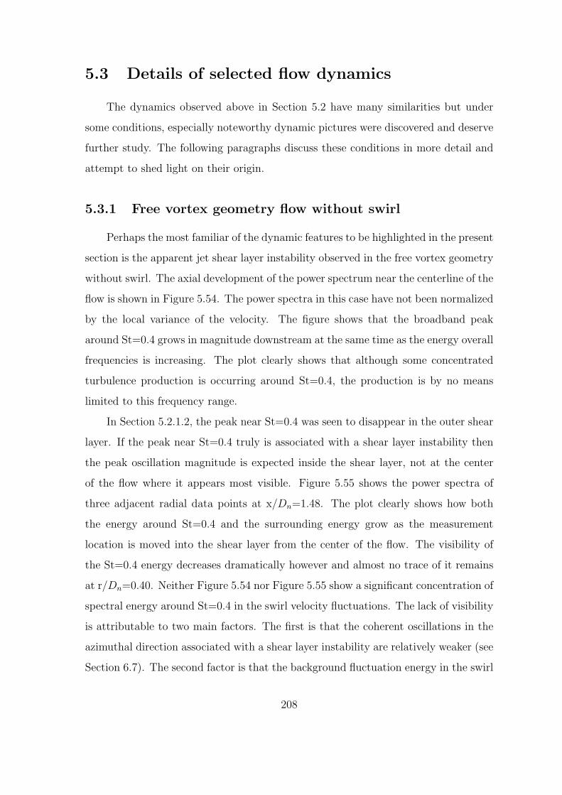
5.3 Details of selected flow dynamics

The dynamics observed above in Section 5.2 have many similarities but under

some conditions, especially noteworthy dynamic pictures were discovered and deserve

further study. The following paragraphs discuss these conditions in more detail and

attempt to shed light on their origin.

5.3.1 Free vortex geometry flow without swirl

Perhaps the most familiar of the dynamic features to be highlighted in the present

section is the apparent jet shear layer instability observed in the free vortex geometry

without swirl. The axial development of the power spectrum near the centerline of the

flow is shown in Figure 5.54. The power spectra in this case have not been normalized

by the local variance of the velocity. The figure shows that the broadband peak

around St=0.4 grows in magnitude downstream at the same time as the energy overall

frequencies is increasing. The plot clearly shows that although some concentrated

turbulence production is occurring around St=0.4, the production is by no means

limited to this frequency range.

In Section 5.2.1.2, the peak near St=0.4 was seen to disappear in the outer shear

layer. If the peak near St=0.4 truly is associated with a shear layer instability then

the peak oscillation magnitude is expected inside the shear layer, not at the center

of the flow where it appears most visible. Figure 5.55 shows the power spectra of

three adjacent radial data points at x/Dn=1.48. The plot clearly shows how both

the energy around St=0.4 and the surrounding energy grow as the measurement

location is moved into the shear layer from the center of the flow. The visibility of

the St=0.4 energy decreases dramatically however and almost no trace of it remains

at r/Dn=0.40. Neither Figure 5.54 nor Figure 5.55 show a significant concentration of

spectral energy around St=0.4 in the swirl velocity fluctuations. The lack of visibility

is attributable to two main factors. The first is that the coherent oscillations in the

azimuthal direction associated with a shear layer instability are relatively weaker (see

Section 6.7). The second factor is that the background fluctuation energy in the swirl

208

10-2

10-1

100

101

10-6

10-5

10-4

10-3

10-2

10-1 Axial Velocity


Po

wer

sp

ectr

al d

ensi

ty (

m2 /sec

2 /Hz)

x = 0.97x = 1.48x = 2.00x = 3.14

10-2

10-1

100

101

10-6

10-5

10-4

10-3

10-2

10-1 Swirl Velocity

Strouhal number (f*D/U - f(Hz))P

ow

er s

pec

tral

den

sity

(m2 /s

ec2 /H

z)

x = 0.97x = 1.48x = 2.00x = 3.14

Figure 5.54: Axial development of St=0.4 instability at the center of the flow fieldr/Dn=0, Q=50 SCFM

velocity component is higher than that in the axial velocity component in the inner

parts of the flow field thus masking a possible concentration of energy around St=0.4.

To obtain a measure of the radial distribution of the St=0.40 energy, a peak

search in the combustor section spectra was performed. If a peak was found, an esti-

mate of the amplitude was obtained by taking the peak and subtracting an estimate

of the background energy. If no peak was found, the amplitude was set to zero. Fig-

ure 5.56 shows the radial distribution of the St=0.40 amplitudes at all axial locations

measured. The figure shows that as the shear layer is approached, the peak loses

visibility and the amplitudes are calculated to be zero. As long as the peak remains

visible however, it shows a an increase towards the shear layer, as expected. The

radial extent over which the peak is visible is largest upstream and decreases with

increasing distance downstream. The visibility is decreasing due to the spreading of

the turbulence energy from the center of the shear layer to the inner part of the flow

field. Note that the St=0.4 peak is barely visible at all at the first axial location

measured. This indicates that the energy at St=0.4 also requires some axial distance

209

10-2

10-1

100

101

10-6

10-5

10-4

10-3

10-2

10-1 Axial Velocity


Po

wer

sp

ectr

al d

ensi

ty (

m2 /sec

2 /Hz)

r = 0.33r = 0.36r = 0.40

10-2

10-1

100

101

10-6

10-5

10-4

10-3

10-2

10-1 Swirl Velocity


ow

er s

pec

tral

den

sity

(m2 /s

ec2 /H

z)

r = 0.33r = 0.36r = 0.40

Figure 5.55: Radial ”cut-off” of St=0.4 instability, x/Dn=1.48, Q=50 SCFM

to generate enough energy in the center of the flow to become visible against the

background turbulence.

The main point to be made here regarding flow development is that although the

flow is relatively efficient at producing broadband turbulence, the energy produced

stays local to the shear layer for a relatively long period of time. The St=0.4 energy

however appears relatively quickly at the center of the flow field and therefore is most

visible here. From a mixing point of view, the apparent instability is a much more

efficient mechanism of transport of momentum than the broadband localized shear

layer turbulence production.

To further describe the axial growth of the energy around St=0.4, Figure 5.57

plots the amplitude of the St=0.4 peak as a function of the axial coordinate near the

center of the flow. The plot shows that the rate of energy gain increases slightly and

then remains linear. Linear growth in energy means that the linear amplitude of the

associated wave is growing only as the square root of the axial coordinate. The lower

than exponential growth is expected in this part of the flow field, as shown in Cohen

and Wygnanski (1987b). Exponential growth only occurs in the initial part of flow

210

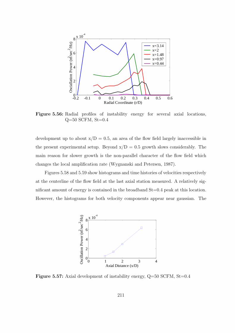
-0.2 -0.1 0 0.1 0.2 0.3 0.4 0.5 0.60

2

4

6

8x 10

-4

Radial Coordinate (r/D)

Osc

ialla

tion

Po

wer

(m2 /s

ec2 /H

z)

x=3.14x=2 x=1.48x=0.97x=0.44

Figure 5.56: Radial profiles of instability energy for several axial locations,Q=50 SCFM, St=0.4

development up to about x/D = 0.5, an area of the flow field largely inaccessible in

the present experimental setup. Beyond x/D = 0.5 growth slows considerably. The

main reason for slower growth is the non-parallel character of the flow field which

changes the local amplification rate (Wygnanski and Petersen, 1987).

Figures 5.58 and 5.59 show histograms and time histories of velocities respectively

at the centerline of the flow field at the last axial station measured. A relatively sig-

nificant amount of energy is contained in the broadband St=0.4 peak at this location.

However, the histograms for both velocity components appear near gaussian. The

0 1 2 3 40

2

4

6

8x 10

-4

Axial Distance (x/D)

Osc

illat

ion

Po

wer

(m2 /s

ec2 /H

z)

Figure 5.57: Axial development of instability energy, Q=50 SCFM, St=0.4

211

0.9 1 1.1 1.20

0.5

1

Axial Velocity

Normalized Velocity

Per

cen

t of D

ata

Po

ints

-0.1 0 0.10

0.5

1

Swirl Velocity

Normalized Velocity

Per

cen

t of D

ata

Po

ints

Figure 5.58: Histogram of velocities, r/Dn=0.02, x/Dn=3.14, Q=50 SCFM

0 0.1 0.20.9

1

1.1

1.2

1.3Axial Velocity

Time (sec)

Vel

oci

ty (

m/s

ec)

0 0.1 0.2-0.2

-0.1

0

0.1

0.2Swirl Velocity

Time (sec)

Vel

oci

ty (

m/s

ec)

Figure 5.59: Time history of velocities, r/Dn=0.02, x/Dn=3.14, Q=50 SCFM

St=0.4 energy peak is too broadly distributed in frequency to generate the bi-modal

distribution that would be observed for velocity data with significant periodic con-

tent. The sample time history of axial velocity fluctuations shown in Figure 5.59

shows more evidence of coherent fluctuations. The period of the relatively noisy os-

cillation, is near the expected frequency of approximately 40 Hz. It is clear from

these plots though that the background turbulence modulates the main oscillation

and interacts with it. The turbulence is not merely superimposed on the oscillation.

Although the dynamics observed around St=0.4 for the zero swirl case are not

very spectacular, they do lend significant insight into how flows with significant input

turbulence exhibit traces of convective instability. In the presence of significant inlet

turbulence, the action of the instability may be masked by broadband turbulence pro-

212

duction in some areas of the flow but visible in other parts. Visibility of concentrated

spectral energy does not imply that the origin of the concentrated spectral energy is

near. The actual amplitude distribution of the energy must be determined in order to

make an assessment on the origin. In the present flow, the instability is most visible

in the center of the flow but clearly originates in the outer shear layer, where it is

however masked by concurrent broad band turbulence production.

The introduction of swirl adds shear to the center of the flow field and hence

turbulence production. It is likely that convective instabilities are still active when

swirl is present but that their effect is masked by efficient swirl induced turbulence

production in conjunction with broadband turbulence production in the outer shear

layer.

5.3.2 Annulus geometry oscillations at higher swirl numbers

Compared to the dynamics of the jet flow just described, the dynamics observed

at S=0.60 in the annulus geometry are of much larger scale. Large narrow band

spectral peaks are observed in the initial development region of the flow field. The

associated mean velocity field exhibits a ring jet with a large central recirculation

zone. Although both axial and swirl velocity fluctuations show evidence of the ap-

parent flow instability, the distribution of oscillation amplitudes shown in Figure 5.60

differs significantly between the two velocity components. The amplitude distribu-

tion very clearly shows the existence of nodes along the radial direction where the

instability is essentially absent. The axial oscillation amplitude has nodes at the flow

center, at around r/Dh=0.75 and just beyond r/Dh=1. The swirl oscillation ampli-

tude distribution only has one clear node at r/Dh=0.25. The instability is not visible

in the axial or swirl velocity fluctuations in the outer recirculation zone.

As the flow develops downstream, the axial velocity oscillation magnitude first

increases and then decreases. The swirl oscillation magnitude decreases. The nodes

of the distributions remain visible downstream and are stationary in radial location

except for the off-centerline nodes of the axial velocity amplitude distribution. These

nodes move outward. Figure 5.61 shows the axial development of velocity profiles for

213

-0.5 0 0.5 1 1.5 20

0.05

0.1

0.15

0.2

0.25

0.3

0.35

0.4Axial Velocity

Radial coordinate (r/D)

Osc

illat

ion

Po

wer

(m2 /s

ec2 /H

z)x = 0.68x = 0.91x = 1.47

-0.5 0 0.5 1 1.5 20

0.05

0.1

0.15

0.2

0.25

0.3

0.35

0.4Swirl velocity

Radial coordinate (r/D)O

scill

atio

n P

ow

er (

m2 /sec

2 /Hz)

x = 0.68x = 0.91x = 1.47

Figure 5.60: Radial distribution of oscillation magnitude for S=0.6 andQ=50 SCFM

the condition currently discussed. The figure reveals that the movement of the axial

oscillation amplitude nodes matches the change in radial location of the inner and

outer shear layer of the ring jet. Similarly, the swirl velocity does not exhibit a shift

in shear layer location and the nodes are seen to remain stationary. Furthermore,

note that the shear in the swirling flow field at x/Dh=1.48 is significantly lower than

at the other two axial locations and the instability is barely able to be detected in

the swirl velocity oscillations.

The instability is thus closely related to the shear in the axial and swirl velocity

profiles. The striking part about this flow shear related instability is how narrow the

spectral energy distribution is. As observed for the non-swirling jet above, the flow

is expected to amplify disturbances over some relatively broad range of frequencies.

The narrow–band behavior seen here can usually only be obtained by adding exter-

nal excitation to the flow, either artificially using a speaker or naturally, using the

feedback provided by an acoustic mode. To help show that the excitation in this case

is internal, i.e. the flow is self excited, the experimental conditions were varied from

the starting point of S=0.6 and Q=50 SCFM. In Section 5.2.2.2 it was already seen

214

-0.5 0 0.5 1 1.5 2-0.5

0

0.5

1

1.5Axial velocity


No

rmal

ized

vel

oci

tyx = 0.68x = 0.91x = 1.47

-0.5 0 0.5 1 1.5 2

-0.4

-0.2

0

0.2

0.4

0.6

0.8Swirl velocity

Radial coordinate (r/D)N

orm

aliz

ed v

elo

city

x = 0.68x = 0.91x = 1.47

Figure 5.61: Velocity profiles for S=0.6 and Q=50 SCFM

that the frequency appears to scale linearly with flow rate.

Experiments using the custom microphone transducers were performed over a

wide range of flow rate at the same swirl angle setting as for S=0.60. The resulting

frequency dependence is shown in Figure 5.62. The frequencies vary linearly over the

entire range of flow rates. The microphones used in the study were located immedi-

ately downstream of the sudden expansion. Microphones further downstream did not

register the flow oscillation frequency. The fact that downstream microphones did

not register the flow oscillation gives further support to the idea that the oscillation

observed is a self excited flow oscillation, as would be expected from an absolutely un-

stable flow. Chapter 6, in particular Section 6.7 will investigate the absolute stability

characteristics of the mean flow field underlying the self–excited velocity oscillations.

In order to connect the dynamics observed at S=0.60 to those observed at S=0.30,

additional measurements were performed in a range of swirl numbers between 0.18

and 0.91, keeping the flow rate constant at a nominal 50 SCFM. The variation of

the instability frequency with swirl number is shown in Figure 5.63. The variation

215

20 40 60 80 100 120 1400

20

40

60

80

100

120

Flow Rate (SCFM)

Fre

qu

ency

(H

z)Mic. Data Linear Fit

Figure 5.62: Instability frequency vs. flow rate for S=0.60

of frequency is close to linear. Below S=0.35 however, the instability is no longer

visible.

Figure 5.64 shows the radial distribution of the oscillation magnitude for several

swirl numbers. The figure shows that for all swirl numbers the shape of the distribu-

tion is relatively constant. The magnitude of the oscillation however rapidly decreases

between S=0.42 and S=0.36 and is known to be absent for S = 0.30. A significant

outward shift of the distribution is observed as the swirl number increases above 0.60.

0 0.2 0.4 0.6 0.8 10

20

40

60

Swirl Number

Inst

abili

ty F

req

uen

cy (

Hz)

Figure 5.63: Instability frequency vs. swirl number for Q=50 SCFM

216

-0.5 0 0.5 1 1.5 20

0.05

0.1

0.15

0.2

0.25

0.3

0.35

0.4Axial Velocity


Osc

illat

ion

Po

wer

(m2 /s

ec2 /H

z)S = 0.84S = 0.60S = 0.42S = 0.35

-0.5 0 0.5 1 1.5 20

0.05

0.1

0.15

0.2

0.25

0.3

0.35

0.4Swirl velocity

Radial coordinate (r/D)O

scill

atio

n P

ow

er (

m2 /sec

2 /Hz)

S = 0.84S = 0.60S = 0.42S = 0.35

Figure 5.64: Radial distribution of oscillation magnitude for several swirl numbersat x/Dh=0.68, Q=50 SCFM

The S=0.84 case shows very clearly that there is a second interior instability node.

At the other swirl levels, the node is either absent or very faint.

The velocity profiles corresponding to Figure 5.64 are shown in Figure 5.65. In

comparing the two figures it is once again clear that the oscillation peaks correspond

closely with the inner and outer shear layers. The strong outward shift of the swirl

velocity profile at S=0.84 is very noticeable. The accompanying increased width of

the central shear shear layer is reflected in a wider oscillation distribution peak at

the center of the flow. The axial velocity profiles show that reverse flow is covering

a significant part of the inlet at S=0.84. Indeed, even the nozzle velocity profile at

x/Dh=-0.53 shows some signs of reverse flow reaching into the nozzle section. The

result of flow detaching from the inner center–body is an accelerated consumption of

azimuthal momentum in this zone, leading to the increased thickness in the central

shear layer observed in the combustor section swirl velocity profile.

Figures 5.66 and 5.67 show velocity time histories and histograms respectively at

r/Dh=0.5, x/Dh=0.68 for S=0.6, Q=50 SCFM. The sample time histories shown in

217

-0.5 0 0.5 1 1.5 2

-0.4

-0.2

0

0.2

0.4

0.6

0.8

1

1.2

Axial velocity


No

rmal

ized

vel

oci

ty

S = 0.84S = 0.60S = 0.42S = 0.35

-0.5 0 0.5 1 1.5 2

-0.4

-0.2

0

0.2

0.4

0.6

0.8Swirl velocity

Radial coordinate (r/D)N

orm

aliz

ed v

elo

city

S = 0.84S = 0.60S = 0.42S = 0.35

Figure 5.65: Velocity profiles for several swirl numbers at x/Dh=0.68, Q=50 SCFM

Figure 5.66 underline the difference between the distribution of swirl and axial velocity

oscillation magnitudes. At r/Dh=0.5, the axial velocity oscillation magnitude is near

its maximum whereas the swirl velocity oscillation magnitude is near its innermost

node. The time history shows a vigorous oscillation with significant recirculation in

the low part of the cycle. The swirl velocity on the other hand appears relatively

quiet and exhibits no sign of coherent oscillation. The picture obtained from the time

histories is reinforced by the histograms shown in Figure 5.67. The axial velocity

histogram shows a very wide distribution with two smeared peaks. The bi-modal

distribution is clear evidence of periodic motion. The swirl velocity histogram on the

other hand is near gaussian.

The converse of the conditions in Figures 5.66 and 5.67 is shown in Figures 5.68

and 5.69, which shows time histories and histograms for the same conditions except

at r/Dh=0.02, near the centerline of the flow. The point here is chosen near an axial

velocity fluctuation node and a swirl velocity fluctuation maximum. The time history

now appears more random for the axial velocity component and distinctively periodic

for the swirl velocity component. The histograms are less easily distinguished. The

218

0 0.1 0.2-1

-0.5

0

0.5

1

1.5Axial Velocity

Time (sec)

Vel

oci

ty (

m/s

ec)

0 0.1 0.2-1

-0.5

0

0.5

1

1.5Swirl Velocity

Time (sec)

Vel

oci

ty (

m/s

ec)

Figure 5.66: Time histories of axial and swirl velocity at r/Dh=0.50, x/Dh=0.68,S=0.6, Q=50 SCFM

-1 0 1 20

0.2

0.4

0.6

0.8

Axial Velocity

Normalized Velocity

Per

cen

t of D

ata

Po

ints

0 0.5 1 1.50

0.5

1

Swirl Velocity

Normalized Velocity

Per

cen

t o

f Dat

a P

oin

ts

Figure 5.67: Histograms of axial and swirl velocity at r/Dh=0.50, x/Dh=0.68,S=0.6, Q=50 SCFM

219

0 0.1 0.2-1

-0.5

0

0.5

1

Axial Velocity

Time (sec)

No

rmal

ized

Vel

oci

ty

0 0.1 0.2-1

-0.5

0

0.5

1

Swirl Velocity

Time (sec)

No

rmal

ized

Vel

oci

ty

Figure 5.68: Time history of velocity at r/Dh=0.02, x/Dh=0.68, S=0.6,Q=50 SCFM

-1 -0.5 0 0.50

0.5

1

1.5

Axial Velocity

Normalized Velocity

Per

cen

t of D

ata

Po

ints

-1 0 10

0.2

0.4

0.6

0.8

1

Swirl Velocity

Normalized Velocity

Per

cen

t of D

ata

Po

ints

Figure 5.69: Histograms of axial and swirl velocity at r/Dh=0.02, x/Dh=0.68,S=0.6, Q=50 SCFM

swirl velocity histogram does not appear bi-modal although it does appear much

wider than in Figure 5.67. The axial velocity distribution is narrower but still exhibits

evidence of other than random dynamics with a secondary peak in the histogram.

The high degree of similarity seen in the instability structure under variation

of swirl and the smooth linear variation of frequency with flow rate all support the

diagnosis that the oscillations observed are due to a flow instability that is self-excited.

The gain provided by acoustic feedback is too sensitive a function of frequency to

allow the instability frequency to vary linearly with flow rate over the wide range

220

reported here. There is the possibility that the oscillations represent the response

of a very narrow band lightly damped resonance to broad band turbulence input.

Such resonances have indeed been found for separated flows. Cooper and Crighton

(2000) showed that jet instabilities can be modeled as damped absolute resonances.

The resonance then relies on the existence of a damped global mode. In determining

absolute stability in Chapter 6, the existence of global modes will be determined.

5.3.3 Annulus geometry dynamics at lower swirl numbers

As swirl is decreased the neatly organized instability discussed in Section 5.3.2 is

replaced by a very complex dynamic picture. The discussion will center around the

S=0.30 case of the annulus geometry. The velocity profiles for this case at 50 SCFM

are shown for the first three measured axial stations in Figure 5.70. The velocity

profiles at 100 SCFM are very similar and will not be repeated here (see Section 4.3).

The plot shows the relatively rapid consumption of azimuthal momentum in the swirl

velocity profiles accompanied by a wake type axial velocity profile that recovers and

widens downstream.

Figure 5.71 shows the un-normalized power spectra at several radial locations

mostly in the inner shear layer (wake). The outermost radial location is just outside

the wake portion of the axial velocity profile. The spectra clearly show how much more

fluctuation energy is contained in the wake portion of the flow field. The broadband

peak mentioned above in Section 5.2.2 is most visible in the swirl velocity fluctuations

but also appears in the axial velocity fluctuations, at radial locations away from the

center of the flow field.

Figure 5.72 and 5.73 show a radial comparison of power spectra at x/Dh=1.47

at S=0.30. Figure 5.72 shows the results for 50 SCFM and Figure 5.73 shows the

results for 100 SCFM. The wake at this axial location has broadened but still exhibits

the same mean axial velocity minimum as x/Dh=0.68. The radial locations at which

the spectra are shown again correspond to locations in the inner shear layer. The

outermost radial location is very near the outer edge of the wake. The results for

the two flow rates are very similar. The downward shift in frequency of the spectral

221

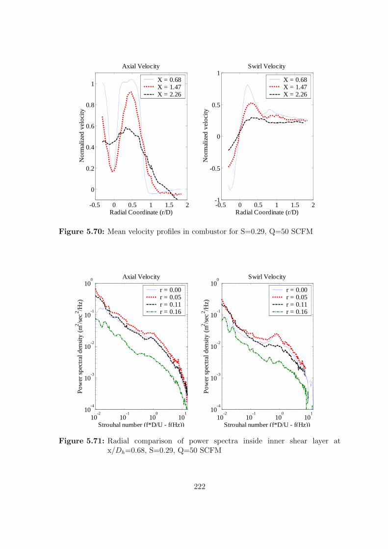
-0.5 0 0.5 1 1.5 2

0

0.2

0.4

0.6

0.8

1

Axial Velocity


No

rmal

ized

vel

oci

tyX = 0.68X = 1.47X = 2.26

-0.5 0 0.5 1 1.5 2-1

-0.5

0

0.5

1Swirl Velocity

Radial Coordinate (r/D)N

orm

aliz

ed v

elo

city

X = 0.68X = 1.47X = 2.26

Figure 5.70: Mean velocity profiles in combustor for S=0.29, Q=50 SCFM

10-2

10-1

100

101

10-4

10-3

10-2

10-1

100 Axial Velocity


Po

wer

sp

ectr

al d

ensi

ty (

m2 /sec

2 /Hz)

r = 0.00r = 0.05r = 0.11r = 0.16

10-2

10-1

100

101

10-4

10-3

10-2

10-1

100 Swirl Velocity


Po

wer

sp

ectr

al d

ensi

ty (

m2 /sec

2 /Hz)

r = 0.00r = 0.05r = 0.11r = 0.16

Figure 5.71: Radial comparison of power spectra inside inner shear layer atx/Dh=0.68, S=0.29, Q=50 SCFM

222

10-2

10-1

100

101

10-4

10-3

10-2

10-1

100 Axial Velocity


Po

wer

sp

ectr

al d

ensi

ty (

m2 /sec

2 /Hz)

r = 0.00r = 0.16r = 0.32r = 0.47

10-2

10-1

100

101

10-4

10-3

10-2

10-1

100 Swirl Velocity


ow

er s

pec

tral

den

sity

(m2 /s

ec2 /H

z)

r = 0.00r = 0.16r = 0.32r = 0.47


peak is observed for both flow rates and the peak is visible in both swirl and axial

velocity fluctuations. The strength of the fluctuations decreases towards the edge of

the wake where the spectral peak is barely visible. The visibility of the peak in the

axial velocity fluctuations is better for the higher flow rate.

Figure 5.74 and 5.75 show a radial comparison of power spectra at x/Dh=2.26 at

S=0.30. Figure 5.74 shows the results for 50 SCFM and Figure 5.75 shows the results

for 100 SCFM. Both figures show that the broadband spectral peak has increased

significantly in width and again shifted lower in frequency, although the shift here is

less than the downward shift between x/Dh=0.68 and x/Dh=1.47. The development

of the spectral energy is consistent with the view introduced above in Section 5.2.2,

based on convective instability considerations. Relatively high frequency amplifica-

tion occurs initially in the flow. Only the lower frequency portion of the energy is

further amplified downstream. Amplification rates decrease in the downstream direc-

tion resulting in a relatively smeared spectral picture. In Section 5.3.1, the spectral

peak was seen to attain its peak magnitude at the last axial station measured. The

223

10-2

10-1

100

10-4

10-3

10-2

10-1

100

101 Axial Velocity


Po

wer

sp

ectr

al d

ensi

ty (

m2 /sec

2 /Hz)

r = 0.00r = 0.16r = 0.32r = 0.47

10-2

10-1

100

10-4

10-3

10-2

10-1

100

101 Swirl Velocity


ow

er s

pec

tral

den

sity

(m2 /s

ec2 /H

z)

r = 0.00r = 0.16r = 0.32r = 0.47


reason for this is the very slow development of the flow field. The speed of develop-

ment here is above that of the jet and as a consequence the spectral peak reaches its

highest visibility relatively early in the flow and becomes smeared downstream. Also

consistent with this picture is the power spectrum observed for the S=0 case in the

annulus geometry (Section 5.2.2). In this case, the flow develops extremely quickly

and no spectral energy concentrations are visible at any axial location.

The other feature of the S=0.30 flow field worthy of more detailed discussion is

the structure of the low frequency energy observed in the flow field. Figures 5.76

and 5.77 show time histories of the velocity near the outer edge of the inner shear

layer. Neither the time scale nor the velocity scale have been normalized for these

plots. The figures show that there is a repeatable pattern for both flow rates. The

pattern period is about 0.75 sec for 100 SCFM and about 2 sec for 50 SCFM. The

frequency thus does not exactly scale with flow rate. The periodicity is observed in

both axial and swirl velocities. The pattern itself however differs greatly between

axial and swirl velocity. At the start of the pattern, the axial velocity decreases

224

10-2

10-1

100

101

10-4

10-3

10-2

10-1

100

101 Axial Velocity


Po

wer

sp

ectr

al d

ensi

ty (

m2 /sec

2 /Hz)

r = 0.00r = 0.16r = 0.32r = 0.47

10-2

10-1

100

101

10-4

10-3

10-2

10-1

100

101 Swirl Velocity


ow

er s

pec

tral

den

sity

(m2 /s

ec2 /H

z)

r = 0.00r = 0.16r = 0.32r = 0.47


10-2

10-1

100

10-4

10-3

10-2

10-1

100 Axial Velocity


Po

wer

sp

ectr

al d

ensi

ty (

m2 /sec

2 /Hz)

r = 0.00r = 0.21r = 0.32r = 0.53

10-2

10-1

100

10-4

10-3

10-2

10-1

100 Swirl Velocity


Po

wer

sp

ectr

al d

ensi

ty (

m2 /sec

2 /Hz)

r = 0.00r = 0.21r = 0.32r = 0.53


225

0 1 2 3-5

0

5

10Axial Velocity

Time (sec)

Vel

oci

ty (

m/s

ec)

0 1 2 3-2

0

2

4

6

8Swirl Velocity

Time (sec)

Vel

oci

ty (

m/s

ec)

Figure 5.76: Intermittence at x/Dh=1.47, r/Dh=0.34, S=0.29, Q=50 SCFM

0 0.5 1 1.5 2-10

0

10

20Axial Velocity

Time (sec)

Vel

oci

ty (

m/s

ec)

0 0.5 1 1.5 2-5

0

5

10

15Swirl Velocity

Time (sec)

Vel

oci

ty (

m/s

ec)


sharply to negative velocities, indicating reverse flow. At the same time, the swirl

velocity begins to exhibit large oscillations about zero. After a time relatively short

compared to the period of the intermittence, axial velocity increases again sharply

and the swirl velocity ceases to exhibit large magnitude oscillations.

Figure 5.78 shows the structure of the intermittence in the middle of the low

velocity portion of the intermittence for r/Dh=0.42 and x/Dh=1.47 (100 SCFM). Very

large sinusoidal oscillations can be clearly identified, especially in the axial velocity.

The frequency of these oscillations corresponds to the spectral peak observed in the

power spectra at around St=0.4. In between the low velocity portions of the cycle, the

226

0.05 0.1 0.15-5

0

5

10

15Axial Velocity

Time (sec)

Vel

oci

ty (

m/s

ec)

0.05 0.1 0.15-2

0

2

4

6

8

10Swirl Velocity

Time (sec)V

elo

city

(m

/sec

)


data rate of the LDV is slowed considerably, but these coherent oscillations cannot be

distinguished in the high velocity portion of the intermittence. The high coherence of

oscillations observed in Figure 5.78 is not typical. At other radial locations the sample

time histories show only limited evidence of the coherent sinusoidal oscillations.

The form of the intermittence is a sensitive function of the radial location.

Figure 5.79 shows sample time histories of velocity for the 50 SCFM flow rate at

r/Dh=0.16, x/Dh=1.47. Figure 5.80 shows sample time histories of velocity for the

100 SCFM flow rate at r/Dh=0.68, x/Dh=1.47. The intermittence in these figures

looks nearly sinusoidal with periods still matching those seen above. It is interesting

to note that for Figure 5.80, the swirl velocity does not exhibit any signs of intermit-

tence.

The various time histories of velocity shown above can be attributed to periodic

radial movement of the flow exiting from the nozzle. The movement is such that the

actual flow structure stays intact. The radial movement of the flow causes a point

measurement of velocity to exhibit the intermittence observed above. For points near

the edge of the wake (Figures 5.76 and 5.77), the velocity will appear near constant as

227

0 1 2-5

0

5

Axial Velocity

Time (sec)

Vel

oci

ty (

m/s

ec)

0 1 2-4

-2

0

2

4

6

Swirl Velocity

Time (sec)

Vel

oci

ty (

m/s

ec)


0 0.5 1-5

0

5

10

15

20Axial Velocity

Time (sec)

Vel

oci

ty (

m/s

ec)

0 0.5 1-5

0

5

10

15Swirl Velocity

Time (sec)

Vel

oci

ty (

m/s

ec)


228

the flow moves radially inward because the mean velocity profile is flat in this region.

As the flow moves radially outward however, the velocity decreases rapidly, causing a

dip in the time history of axial velocity. The swirl velocity associated with the wake

part of the flow is much more turbulent and hence the swirl velocity exhibits high

amplitude fluctuations when the axial velocity has dipped down.

Also consistent with this picture is the fact that the sinusoidal velocity oscillations

are observed in the wake portion of the jet movement cycle. The sinusoidal velocity

fluctuations are associated with the inner shear layer instability and are especially

visible in the wake. Away from the edge of the shear layer, the pattern becomes more

sinusoidal as the mean velocity profile becomes more linear. The r/Dh=0.68 point is

located in the middle of the outer shear layer and therefore exhibits nearly sinusoidal

oscillations in axial velocity. The swirl velocity time history shows no clear evidence

of jet movement since the mean velocity here is nearly flat. The point r/Dh=0.16

is located in the middle of the inner shear layer and therefore also exhibits nearly

sinusoidal oscillation. At r/Dh=0.16, oscillation is also observed in the swirl velocity

time history because the point is located in the middle of the vortex core of the mean

swirl velocity profile.

Figure 5.79 shows the time histories of velocity for r/Dh=0.16, x/Dh=0.68 at

50 SCFM. The point is chosen near the edge of the inner shear layer, similar to location

r/Dh=0.34 at x/Dh=1.48. Once more, intermittence can be observed in the flow field.

However, the magnitude of the intermittence is much lower than observed further

downstream. The lower magnitude of the intermittence is noteworthy especially in

view of the fact that the velocity profiles are steeper at x/Dh=0.68 than x/Dh=1.48.

For the same amount of movement, a larger intermittence would be expected at

x/Dh=0.68. The fact that the intermittence is weaker at x/Dh=0.68 points to the

fact that the jet movement decreases upstream. A likely anchor point for the jet

movement is the dump location into the downstream section where the flow leaves

the center–body.

Intermittence is also observed downstream of x/Dh=1.48, but the magnitude and

coherence of the patterns decreases significantly. The motion of the jet is less notice-

229

0 0.5 1 1.50

2

4

6

8

10

Axial Velocity

Time (sec)

Vel

oci

ty (

m/s

ec)

0 0.5 1 1.5

0

2

4

6

8

Swirl Velocity

Time (sec)

Vel

oci

ty (

m/s

ec)


able downstream due to the decreased velocity gradients in the flow field. Clearly,

the jet movement plays a pivotal role in the rapid mixing required to cause the ve-

locity gradients to decrease so quickly. In Section 5.2.2 it was noted that the S=0.30

case flow field recovers more quickly than the S=0.60 velocity field. The cause of the

accelerated flow development is the very efficient mixing executed by the movement

of jet exiting into the dump. Jet movement is apparently more efficient at achieving

large scale mixing than the large instability observed in the flow field at S=0.60.

Low frequency energy has also been noted under many other conditions flow

conditions, but the large amplitude observed in the present flow field is unique to the

intermediate swirl strength condition. Figure 5.82 shows the time histories of velocity

in the inner shear layer at the same radial location as Figure 5.79 (r/Dh=0.16) but for

the zero swirl condition. No trace of periodic intermittence can be observed, although

the turbulent fluctuations are very high.

The cause of the movement described above is difficult to analyze. The role

of swirl in the flow field cannot be understated however. In order to help point in

the direction of the cause of the movement, Figure 5.83 shows the velocity profiles

for four swirl levels at x/Dh=0.68, Q=50 SCFM. The dependence of the minimum

mean axial velocity on the swirl level is of particular interest. Only the S=0.35 case

exhibits clear flow reversal at the centerline. The next lowest velocity is obtained for

S=0, the case without swirl. For this case the annular jet develops into an ordinary

230

0 1 2

0

2

4

6

Axial Velocity

Time (sec)

Vel

oci

ty (

m/s

ec)

0 0.5 1 1.5 2

-4

-2

0

2

4

Swirl Velocity

Time (sec)

Vel

oci

ty (

m/s

ec)

Figure 5.82: Lack of intermittence for x/Dh=0.68, r/Dh=0.16, S=0, Q=50 SCFM

jet at the last measurement location (x/Dh=4.79) as the wake profile in the center

recovers quickly and axial momentum is lost slowly to the outside region of the flow.

The next lowest mean axial velocity at the centerline is obtained from the S=0.30

case. Finally, the S=0.18 case only exhibits a very small wake at x/Dh=0.68. (The

apparent asymmetry near the centerline is caused by the straight line connection

between relatively coarsely spaced data points, not by actual asymmetry in the data)

The expected behavior would have been a smooth increase of the velocity at the

centerline with decreasing swirl level. The fact that the wake appears to diminish

in strength and then increase in strength as the swirl number decreases indicates

that two competing elements are at work in shaping the flow development. The first

element is the bluff body. The second element is swirl. Swirl is generally thought to

expand the recirculation zone behind bluff bodies. However, this is a simplistic view.

Swirl not only affects the pressure distribution in the flow but also is an excellent

mixer through the turbulence produced by the shear that always exists in a flow with

swirl.

The trend observed in Figure 5.83 can be explained in terms of the two influences

of swirl on the flow field: turbulence production and pressure distribution. As swirl

is increased from zero, the changes observed in the flow field are largely due to the

increased turbulence production obtained through the addition of swirl. As swirl is in-

creased further, turbulence production increases but the pressure distribution induced

231

-0.5 0 0.5 1 1.5 2

-0.2

0

0.2

0.4

0.6

0.8

1

1.2

Axial Velocity


No

rmal

ized

vel

oci

tyS=0.35 S = 0.29S = 0.18S = 0

-0.5 0 0.5 1 1.5 2-1

-0.5

0

0.5

1Swirl Velocity

Radial Coordinate (r/D)N

orm

aliz

ed v

elo

city

S=0.35 S = 0.29S = 0.18S = 0

Figure 5.83: Mean velocity profiles at x/Dh=0.68 for low swirl numbers with flowrate of Q=50 SCFM

by swirl is not significant enough to affect the flow field. The radial distribution of

pressure induced by swirl is negligible relative to axial pressure gradient experienced

by the flow. As swirl is increased further, the radial pressure distribution induced by

the swirling velocity field begins to affect the flow field and eventually dominates the

effect on the flow field. The radial momentum equation under the assumption of zero

radial velocity supports the initial insignificance of pressure effects and their eventual

dominance. The radial momentum equation under the specified assumption reduces

to a relationship that states that the local radial pressure gradient is proportional to

the local swirl velocity squared. This non-linear relationship between swirl velocity

and pressure gradient is consistent with the explanation of flow behavior as swirl is

increased.

In terms of Figure 5.83, the bluff body wake is initially erased more quickly by

the addition of swirl because the increased turbulence enhances mixing and therefore

redistributes momentum more rapidly (S=0.18). As swirl is increased further, the

radial pressure distribution begins to be important in flow development and the bluff

body wake expands and extends further downstream. However, turbulence production

232

remains high because the vortex core remains relatively small with high shear and

only expands slowly downstream. A further increase in swirl causes the flow field to

be dominated by the effect of the radial pressure gradient induced by swirl and a wide

central recirculation region develops. The flow diverges radially outward on entering

the downstream section and is slow to recover as turbulence production has slowed

significantly due to the large expansion of the vortex core and associated reduction

in shear.

The movement of the jet seen for the S=0.29 case could thus be interpreted as the

result of a flow field trying to react to two processes at the same time. A motion cycle

could be described as follows. The flow enters with a tight vortex core and the efficient

turbulence production causes rapid mixing of axial and azimuthal momentum. The

dissipation of azimuthal momentum is rapid enough to generate a significant adverse

pressure gradient on the centerline. The flow reverses on the centerline, expanding

the vortex core upstream and deflecting the incoming jet radially outward. The now

expanded vortex core does not produce enough turbulence to produce the mixing

required to continue the rapid dissipation of azimuthal momentum. The adverse

pressure gradient on the centerline is reduced and the flow field eventually reforms at

its starting point, beginning a new cycle.

The process described in the above paragraph is at this point a very poorly

supported argument but it is difficult to determine what specific types of experiments

may lead to further clarification. It is clear that the data presented is very interesting

from a flow control and mixing optimization point of view. For example, in the future,

it may be possible to mechanically enhance the jet movement with little control effort

and further increase mixing.

Finally, the mechanism for jet movement described is global to the flow field and

linear stability analysis cannot be expected to help validate the mechanism.

233

102

103

10-4

10-2

100

102

104

Frequency (Hz)

Pre

ssu

re P

ow

er D

ensi

tyx = -1.38 x = 0.78 x = 5.86 -5/3 slope

Figure 5.84: Noise spectra at various axial locations for S=0.6 and Q=50 SCFM

5.4 Acoustics and flow dynamics

The problem with discussing pressure measurements in a highly turbulent flow

such as that studied here is the separation of propagating acoustic noise and local hy-

drodynamic noise. For the more complicated environment of an operating gas turbine

combustor, Strahle et al. (1977) attempted to separate flow noise, entropy wave in-

duced noise and direct combustion noise. Multiple point simultaneous measurements

in the combustor near the flame, near the combustor exit and beyond the exit were

able to shed some light on the relative importance of the contributions.

A more qualitative way to distinguish hydrodynamic noise from acoustic noise is

in looking at the frequency content of the noise. Figure 5.84 shows the power spectra

of pressures measured at various axial locations. The nozzle pressure spectrum lies

significantly above that in the downstream section of the combustor. This is expected

based on an approximate balance of acoustic energy between the nozzle and the

combustor section. The area reduction causes the pressure levels inside the nozzle to

be higher than those in the combustor. The microphone located relatively close to

the sudden (x/Dn=0.25) expansion exhibits entirely different behavior. The spectrum

strongly resembles that found in the velocity spectra outside the outer shear layer.

234

A -5/3 slope is indicated on the figure to help make the point that the noise

measured in this area of the flow field is closely related to the velocity fluctuations.

The seemingly unorganized oscillations in energy observed in the nozzle and the

downstream location are due to the influence of acoustic modes which occur regularly

with increasing frequency. The signature of these acoustic modes is much weaker for

the location just beyond the dump. The weaker signature of the acoustic pressure

at this location is surprising considering the measurement location is relatively near

the area expansion which acoustically will look like a pressure antinode. One of the

possible reasons the acoustic peaks are suppressed in this area may be the distortion

of the acoustic field caused by the presence of a highly sheared flow.

The strongest peak in the spectrum is observed near the dominant acoustic mode

of the downstream combustor section, around 106 Hz. The wavelength for this mode

is 3.14 m. The combustor test section length is 0.8 m long, meaning that the mode

can be associated with the quarter wavelength of the combustor test section. To

support this claim, Figure 5.85 shows a plot of the operating deflection shapes at

four frequencies in the combustor. The operating deflection shapes were generated

by exciting the combustor with white noise output from a small speaker mounted in

a threaded hole at the top of the combustor. The shape at 100 Hz clearly indicates a

near quarter wavelength distribution. The reason the amplitude of this mode is lower

here than for example the pressure at 200 Hz has to do with the location of driving

which is suboptimal for the 100 Hz mode and near optimal for the 200 Hz mode.

The other feature seen in Figure 5.84 are the peaks located around 45 and 52 Hz.

The 52 Hz peak is only observed in the nozzle and downstream section indicating that

this energy is likely acoustic in nature. The 45 Hz peak is strongest at the location

just beyond the sudden expansion. It is also visible in the nozzle section. The 45 Hz

peak matches the frequency of the instability observed in this flow field exactly and

therefore is likely due to hydrodynamic noise generated by the instability.

Section 5.3.2 hypothesized that because the swirl RMS velocity is non-zero at

the centerline, the mode of instability must have a nonzero azimuthal wavenumber.

Furthermore, higher azimuthal modes also require that oscillations go to zero at

235

2 4 6 8 100

1

2

3

4

Normalized axial distance

No

rmal

ized

wav

e am

plit

ud

e

100 Hz200 Hz300 Hz400 Hz

Figure 5.85: Operating deflection shapes of combustor pressures at four frequencies

the centerline (see Section 6.2). The only possibility is that the mode is associated

with the first azimuthal mode. The problem that remains is to determine the sense

of propagation of the instability with respect to the predominant swirl direction.

Propagation in the opposite direction of swirl indicates an azimuthal wavenumber of

-1. Propagation with the direction of swirl indicates an azimuthal wavenumber of 1.

Without simultaneous two point measurements, and without the ability to phase

lock azimuthal instabilities to a form of excitation the direction of propagation is

difficult to identify. However, the hydrodynamic noise generated by the instability

can be used to help in the identification. Two of the eight microphones used in the

limited acoustic measurements performed were located near the sudden expansion,

spaced at 90 degrees around the perimeter. Figure 5.86 shows the coherence and

transfer function phase between the two microphones. The coherence between the

two microphones at the frequency of instability is 0.7, which is relatively high consid-

ering the energy at this peak is caused by velocity fluctuations. The phase between

the two microphones is difficult to identify but at the instability frequency, the phase

is clearly positive. The positive phase means that the velocity oscillation is moving

with the direction of the mean swirl and thus indicates that the instability has az-

imuthal wavenumber 1. This finding is consistent with the study of Michalke (1999)

which finds that ring jet type velocity profiles with reverse flow on the centerline are

absolutely unstable with azimuthal wavenumber equal to +1. The absolute stabil-

236

20 40 60 80 100 1200

0.2

0.4

0.6

0.8

1Coherence Plot

Frequency (Hz)

Ord

inar

y C

oh

eren

ce

20 40 60 80 100 1200

20

40

60

80

100Phase delay

Frequency (Hz)P

has

e (d

egre

es)

Figure 5.86: Coherence and phase between two circumferentially spaced micro-phones for S=0.6, Q=50 SCFM

ity characteristics of the flow fields measured here are examined in Section 6.7 of

Chapter 6.

In order to investigate whether or not the instability is an acoustic source in the

flow field, the power contained in the pressure fluctuations around 106 Hz(± 6 Hz) is

plotted against flow rate. The resulting plot is shown in Figure 5.87. The plot shows

that the pressure oscillation power is a rapidly increasing function of flow rate. At

the last flow rate, the instability frequency overlaps with the quarter wave mode of

the combustor. However, no increase in power is seen above that expected for the

increase in flow rate. The inability of the instability to force the 106 Hz mode must

not be attributed to the instability characteristics alone. Clearly the fact that the

instability is azimuthal makes it a relatively inefficient driver. However, nearly as

important is that the 106 Hz mode has a pressure antinode near the instability so

that acoustic velocities are close to zero (at least in the outer parts of the flow field)

and the acoustic mode is not able to be driven efficiently.

237

20 40 60 80 100 120 14010

0

105

Flow Rate (SCFM)

Pre

ssu

re P

ow

er (

Pa

2 )

x = -1.38x = 0.78 x = 3.71 x = 5.86

Figure 5.87: Pressure oscillation power around 100 Hz as a function of flow rate

238

chapter 5 experimental results - dynamics

Documents