chapter 5 first principles potentials for al-(ti, zr)-(ni ... · (thijssen, 1999). subsequently,...

5-1

Chapter 5

First principles potentials for Al-(Ti, Zr)-(Ni, Cu) system

5.1 Introduction

The prediction of materials properties using only first principles has been actively

pursued in computational materials science (Goddard III, 2000). The first principle

method is defined as the method that requires no empirical input and quantum mechanics

(QM) is used as its foundation. QM provides the wave function, which is a solution to

Schrodinger’s equation. From the wave function, all physical properties can be derived.

However, in most cases, the Shrodinger equation cannot be solved analytically. Notable

exceptions are the free particle, harmonic oscillator, and hydrogen atom systems

(Thijssen, 1999). Subsequently, many theories have been developed, such as the Hartree-

Fock theory and density functional theory (DFT) (Thijssen, 1999; Koch, 2001). In

particular, DFT has been shown to be relatively accurate compared to experiments in

calculations of atoms and molecules (Hohenberg and Kohn, 1964; Kohn and Sham,

1965). Despite these successes, the practical applications for DFT have been limited by

time and length scales of QM. To overcome this challenge, a hierarchy of methodologies

has been proposed (Fig. 5-1) (Goddard III, 2000). In this paradigm, the important

physical properties are derived from each step and then subsequently used to obtain

effective parameters for the next step. Based on this approach, we perform first principle

calculations of Al, Ti, Ni, Cu, Zr, and their alloys. The necessary physical properties are

derived from QM and then used as an input to obtain the parameters for molecular

dynamics (MD) simulations. Then, MD simulations are carried out to study the

5-2

thermodynamic properties of the alloys systems. In particular, the glass forming ability

(GFA) is studied to aid the new metallic glass forming alloy development. Using the

packing fraction as an indicator for GFA, MD results show that GFA increases around

Al40Ti10Ni50 and Al20Ti10Ni70 composition in AlTiNi system.

5.2 Quantum mechanics calculations

First, the norm-conserving pseudopotentials are generated for Al, Ti, Ni, Cu, and

Zr using the fhi98PP program (Fuchs and Scheffler, 1999) as shown in Fig. 5-2. The

norm-conserving pseudopotential approach provides an effective and reliable means for

performing DFT calculations (Bockstedte et al., 1997). The important features of this

approach are as follows.

• the core states are assumed to be chemically inert

• the potential does not diverge in the core region

• the wavefunction satisfies the norm-conservation condition

Subsequently, the Gaussian basis sets for the norm-conserving pseudopotentials

are developed. Mathematically and numerically, the Gaussian basis formalism is one of

the most efficient to implement for DFT calculations (Schultz, 2000). Using the

pseudopotentials and Gaussian basis sets as inputs, the QM calculations are carried out

using SeqQuest program (Schultz, 2000). The theoretical basis of SeqQuest is DFT with

the local density approximation (LDA) or generalized gradient approximation (GGA).

LDA assumes the constant electron gas density, which is a fairly good approximation for

simple metals such as sodium. GGA accounts the non-homogeneity of the true electron

density by including the gradients of the charge density in calculations. LDA is known to

5-3

underestimate bond lengths or lattice parameters in crystals, while GGA overcorrects the

shortcomings of LDA (Thijssen, 1999). In this thesis, we have used GGA to calculate the

properties of simple metal and transition metals in the framework of DFT.

The energy as a function of atomic volume of the system is obtained using QM.

The obtained relationship between energy and volume is called the equation of state

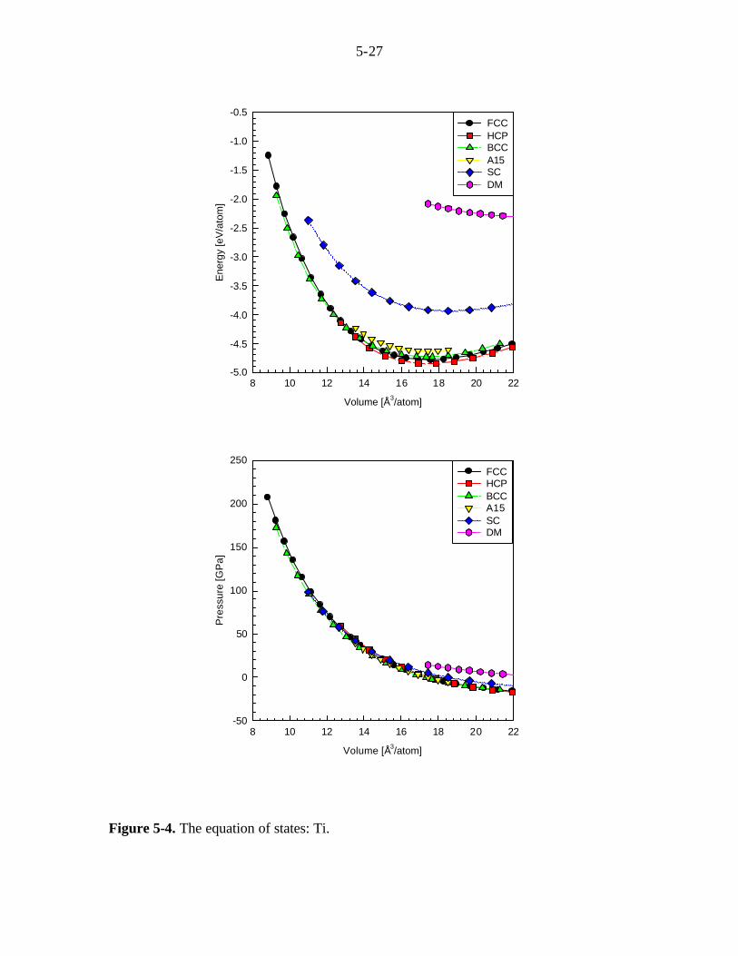
(EOS). We have calculated the EOS of 6 different crystalline phases for Al, Ti, Ni, Cu,

Zr: FCC, HCP, BCC, A15, simple cubic (SC), and diamond (DM). The result for Al is

shown in Fig. 5-3 and the equilibrium data of each phase are summarized in Table 5-1(a).

The equilibrium properties are derived from the QM results using a universal energy

function (Rose et al., 1984). The EOS and equilibrium properties for Ti (Fig. 5-4 and

Table 5-2(a)), Ni (Fig. 5-5 and Table 5-3(a)), Cu (Fig. 5-6 and Table 5-4(a)), and Zr (Fig.

5-7 and Table 5-5(a)) are shown in the same manner. The QM results and experimental

data show good agreement (Table 5-6).

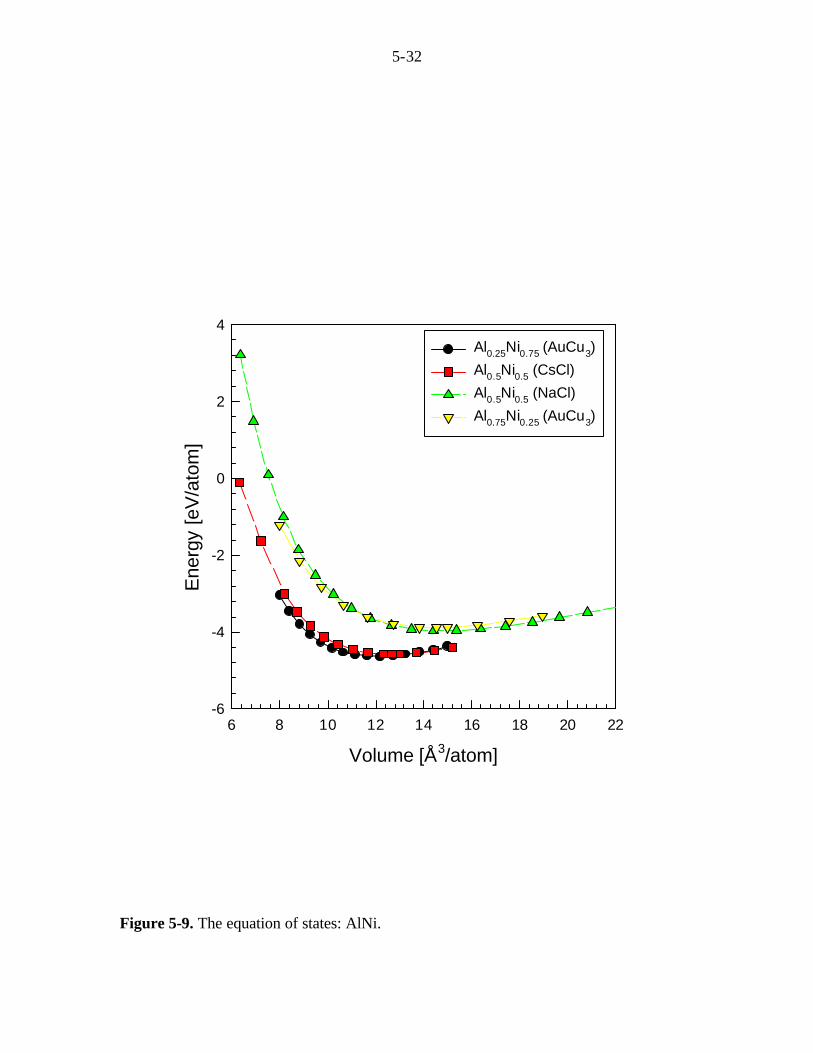
The EOS of alloy phases, such as AlxTi1-x, AlxNi1-x, and TixNi1-x, are also

obtained. The alloys structures employed in this study are AuCu3 for x=0.25 and x=0.75.

For x=0.50, CsCl and NaCl structures are used. The EOS and equilibrium data for

AlxTi1-x, AlxNi1-x, and TixNi1-x are shown in Fig. 5-8, Table 5-7(a), Fig. 5-9, Table 5-8(a),

Fig. 5-10, and Table 5-9(a), respectively. The QM calculations of alloy phases show

good agreement with the available experimental data, such as the lattice constant and the

heat of formation (∆H) (Hultgren, 1973; Villars, 1991).

5-4

5.3 The force-field parameters for pure metals

As introduced in Chapter 1, the Sutton-Chen potential describes the energy U of

atom i as (Sutton and Chen, 1990)

mN

ij ij

ijiii

nN

ij ij

ijiji r

cr

U ∑∑≠≠

−

=

αε

αε

21

. (5-1)

In a pure system, the Eq. 5-1 can be simplified as

m

N

ij ij

nN

ij iji r

cr

U ∑∑≠≠

−

=

αε

αε

21

. (5-2)

Here, ijr is the distance between atom i and j. ε sets the overall energy scale, c is a

dimensionless parameter scaling the attractive term and α is a length parameter.

Since Eq. 5-2 contains a lattice sum such as Sn= ∑≠

N

ij

n

ijrα , it is convenient to

introduce quantities dij such that rij = α0dij, where α0 is the lattice constant of an FCC

crystal. In this work, we restrict the lattice sums to rij=2α0 so that we can include up to

the 8th nearest neighbors (N=140) interactions of an FCC crystal in calculating the

potential function. Thus, dij=22

, 1, ,26

2 , 5.2 , 3 , 214

, 2.

Using dij, Sn can be written as

∑ ∑∑≠ ≠≠

=

=

=

N

ij

N

ij

n

ij

nn

ij

nN

ij ijn ddr

S1

00 αα

ααα

. (5-3)

If we set α equal to α0, Sn is simplified to

∑≠

=

N

ij

n

ijn d

S 1 . (5-4)

5-5

Then the Eq. 5-2 can be rewritten as

mni ScSU εε

−=2

. (5-5)

Since parameter α is determined as α0 for the convenience of the lattice sum,

other force field parameters such as ε, c, m, and n in Eq. 5-5 should be determined

subsequently to satisfy the material properties that we are interested in. To do so, let’s

first consider three fundamental equilibrium material properties such as cohesive energy

Ecoh, atomic volume Ω, and bulk modulus B, which are expressed as following equations

mncohri ScSEU εε

α−=−=

= 20, (5-5)

02

112

13

13

0020

20

0

=

+−−=

∂∂

−=Ω∂

∂−=

=

mnatom

r

iatomi

Sm

cnSN

rUNU

P

αε

αε

α

αα , (5-6)

+−+=

∂∂

=Ω∂

∂Ω=

=

mnatom

r

iatomi

SmmcSnnN

rENU

B

122

1)1(12

19

19

20

200

2

2

02

0

αε

αε

α

αα . (5-7)

Here, P is pressure and Νatom is an integer number such that atomN

30α

=Ω . Then, the Eq. 5-

5~5-7 can be simplified to

m

n

Sm

nSc = , (5-8)

n

coh

SE

mnm

−=

22

ε , (5-9)

5-6

cohEB

nmΩ

=18

. (5-10)

Therefore, if we choose ε, c, m, and n that satisfies Eq. 5-8~5-10, the potential function

Eq. 5-2 automatically reproduces given Ecoh, Ω, and B accurately. However, we have

only 3 equations for 4 parameters so far. Thus, we need additional material properties to

determine the FF parameters.

Previously, Sutton and Chen used elastic constants Cij of materials as additional

material properties to choose the best FF parameter set (Sutton and Chen, 1990). First,

they reduced the number of FF parameter candidate sets by restricting n and m only to

integer numbers that closely satisfy Eq. 5-10. As a result, the potential function fails to

describe B exactly. Then, ε, c are determined using Eq. 5-8 and 5-9. Using the obtained

FF parameter sets, Cij are calculated and compared to the experimental values. The best

FF parameter set is chosen as the one that gives the closest agreement with the

experimental Cij values.

Instead of using Cij, we use the EOS data obtained from QM to determine the best

FF parameter set. The procedure is as follows. First, α is set to the lattice constant of

FCC phase obtained from QM. Then Ecoh_FCC, ΩFCC, and BFCC, which are also obtained

from QM, are used to define relationships among ε, c, m, and n (Eq. 5-8~5-10). Here, we

allow non- integer m and n to have more accurate description of B. Finally, to determine

the best FF parameter set, we use the following QM results.

• The energy-volume curve of FCC phase

• The pressure-volume curve of FCC phase

• The Ecoh of HCP, BCC, A15, SC, DM phases

5-7

• The Ω of HCP, BCC, A15, SC, DM phases

This is accomplished by using the cost function:

∑ ∑∑∑= =

∆+∆+∆+∆=5

1

5

1

)()(k k

Pk

FFk

Uk

FFk

Pi

Vi

FFFCC

Ui

Vi

FFFCC wPwUwVPwVUC

ii

, (5-11)

where ∆UFCCFF(Vi)=UFCC

FF(Vi)-UFCCFF(ΩFCC)=UFCC

FF(Vi)+Ecoh_FCC,

∆PFCCFF(Vi)=PFCC

FF(Vi)-PFCCFF(ΩFCC)= PFCC

FF(Vi),

∆UkFF=Uk

FF(Ωk)-UFCCFF(ΩFCC)= Uk

FF(Ωk)+Ecoh_FCC,

∆PkFF=Pk

FF(Ωk)-PFCCFF(ΩFCC)= Pk

FF(Ωk),

)(/(1 iQMFCC

Pi VUw ∆= , P

iUi ww 100= ,

QMk

Pk Uw ∆= /1 , P

kUk ww 100= ,

0.83843Ω≤Vi≤Ω and k=HCP, BCC, A15, SC, DM.

The superscript FF means the results obtained from FF and QM means the results

obtained from QM. The each term in Eq. 5-11 represents the contributions from QM

results, which are described above in order, in the optimization process of FF parameters.

wiP , wi

U , wkP , and wk

U are weighting functions in the cost function, which are inversely

proportional to the energy difference with the stable FCC phase. In this way, we give

more importance to the low energy phase. Also we set the weighting function ratio

between U and P as 100, because the U and P scales about O(102) in units that we use in

this study (Fig. 5-3~5-7).

Following the procedure described above, force field parameters are optimized to

fit the SC potential based on QM results. The obtained force field parameters are shown

in Table 5-1(b)~5-5(b) for Al, Ti, Ni, Cu, and Zr, respectively. The comparisons between

the FF results and the QM results for each phases are shown in Table 5-1(c)~5-5(c). As

5-8

we expect, the FF describes the lower energy phases more accurately than the higher

energy phases.

5.4 The force-field parameters for alloys

In a binary A-B alloy system, there are A-A, B-B and A-B interactions. A-A and

B-B interactions can be described by using the force-field parameters obtained from pure

A system and pure B system. To accurately describe an A-B interaction, the force field

parameter set (αAB, εAB, cAB, mAB and nAB) for A-B interaction is also needed. Previously,

this was determined by the following expressions, which is called the mixing rule

(Rafiitabar and Sutton, 1991):

BBAAAB ααα = , (5-12)

BBAAAB εεε = , (5-13)

( )2

BBAAAB

mmm

+= , (5-14)

( )2

BBAAAB

nnn

+= , (5-15)

where αAA, εAA, mAA and nAA are respectively α, ε, m and n of the pure A system.

Similarly, αBB, εBB, mBB and nBB are α, ε, m and n of the pure B system. Note that there is

no mixing rule for c because c is assumed to be dependent only on the type of the atom at

which the local energy is evaluated (Sutton and Chen, 1990).

To accurately describe the A-B interaction, we allow that c and ε in the second

term of Eq. 5-1 depends also on the type of interaction. Then, the modified the SC

potential for alloy system can be obtained as:

5-9

m

N

ij ij

ijijij

nN

ij ij

ijiji r

cr

U ∑∑≠≠

−

=

αε

αε 22

21

(5-16)

Consider now AxB1-x binary alloy system. The energy of atom A in site i is

written as:

ABAB

AAAA

ABABAAAA

m

ij

N

ijAj

mAB

ABAB

m

ij

N

ijAj

mAA

AAAA

n

ij

N

ijAj

nABAB

n

ij

N

ijAj

nAAAA

A

dLc

dLc

dLdLU

−

+

−

−

+

=

∑∑

∑∑

≠≠

≠≠

1)1(

1

1)1(

21

2

2222 δα

εδα

ε

δαε

δαε

, (5-17)

and the energy of atom B in site i is written as:

ABAB

BBBB

ABABBBBB

mN

ij ijAj

mAB

ABAB

mN

ij ijAj

mBB

BBBB

nN

ij ijAj

nABAB

n

ij

N

ijAj

nBBBB

B

dLc

dLc

dLdLU

∑∑

∑∑

≠≠

≠≠

+

−

−

+

−

=

11)1(

12

1)1(

2

2222 δα

εδα

ε

δαε

δαε

, (5-18)

where δΑj is 1 if site j is occupied by an A atom or else 0. Then, the total atomic energy

of the AxB1-x binary alloy system is

BA UxxUU )1( −+= (5-19)

Subsequently, the pressure of the AxB1-x binary alloy system is

ABAB

BA

AB

atom

AB

atom Ux

Ux

NUNP

ααααααααα

==

∂∂

−+∂

∂−=

∂∂

−= )1(1

31

3 22 (5-20)

Here, aAB is the lattice constant of the AxB1-x unit cell.

Using the QM calculation results for alloy phases (Table 5-7(a)~5-9(a) and Fig. 5-

8~5-10) and the Eq. 5-19~5-20, the FF parameters for A-B interactions are obtained. The

procedure is as follows. First, the cost function is defined as:

5-10

∑ ∑ −+−=k k

QMk

FFk

QMk

FFk PPUUC 100 , (5-21)

where k=A3B1(AuCu3 structure), AB(NaCl structure), AB(CsCl structure), AB3(AuCu3

structure). Then, the FF parameter set that minimizes the cost function is found. In this

optimization process, the mixing rule is used as an initial guess. Since there is no mixing

rule for cAB, we use BBAAAB ccc = as an initial guess. The next FF parameter set is

defined by changing the previous FF parameters by –δ, 0, and +δ. Ideally, δ should be

chosen considering the overall scale of each parameter. However, we use the uniform

δ=10-5 for all FF parameters in this work. By changing each FF parameters by –δ, 0, and

+δ, 35 FF parameter sets are generated. Among these, the FF parameter set that

minimizes the cost function is selected for the next step. This procedure continues until

the FF parameter set converges. The obtained parameters are summarized in Table 5-

7(b)~5-9(b). The comparisons are made between the force field results and the QM

results, shown in Table 5-7(c)~5-9(c).

5.5 The extension to ternary systems

Using the developed FF parameter set (Table 5-1(b)~5-3(b) and 5-7(b)~5-9(b)),

the MD simulations are done on binary, ternary, and higher order systems. The direct

comparison between the QM calculations and the force-field results should be made to

validate this extension to higher order systems.

In this work, the system of interest is the Al-Ti-Ni ternary system. The aluminum

based intermetallics, such as Al-Ti and Al-Ni, are known to have high strength, high

thermal stability, and high oxidation resistance. Therefore, our objective is to understand

5-11

and predict the phase behavior of Al-Ti-Ni system to guide the better alloy development,

particularly, metallic glasses.

Starting from the random FCC solid solution, we have melted and quenched the

AlxTiyNi(1-x-y) samples using TtN dynamics (Ray and Rahman, 1984, 1985). Due to the

fast cooling rate (4×1012 K/s), glasses are formed in a very broad regime of the ternary

phase diagram. As the initial estimation of the glass forming ability, we have used the

packing efficiency as our indicator. The packing efficiency is defined as:

total

atom

VV

=φ (5-22)

Here, Vatom is the volume of atoms in the system and Vtotal is the total volume of the

system. For example, FCC system with hard sphere approximation gives φ~0.74 and φ

can increase if the soft sphere approximation is used (Haile, 1997). Also, φ is related to

the free volume of the system by

)1( φ−= totalfree VV , (5-23)

thus, φ can be used in connection with the free volume theory (Cohen and Grest, 1979,

1981) to estimate the glass transition behavior. Or intuitively, if the nature of system is

similar, the less free volume results the high viscosity. Therefore, the system with less

free volume have higher barrier for crystal nucleation, thus, can achieve higher degrees of

supercooling, which increases the GFA.

The calculated packing efficiency in the series of AlxTiyNi(1-x-y) system during the

quenching process is shown in Fig. 5-11. The packing efficiency changes smoothly as a

function of concentrations. We predict that the region with the high packing efficiency

5-12

such Al40Ti10Ni50 and Al20Ti10Ni70 as will show a good glass forming ability, however the

comparable experimental results are not available yet.

5.6 Conclusions

The purpose of this work is to extend the first principle calculations to metallic

alloy system, with an emphasis on obtaining first-principle-based inter-atomic potentials.

We perform accurate QM calculations in the framework of DFT with GGA to develop FF

parameters. Then, the developed FF parameters are employed in MD calculations to

study the thermodynamic properties of AlTiNi metallic alloy system. In particular, the

study is focused on predicting the glass forming ability (GFA) to aid the new metallic

glass forming alloy development. Using the packing fraction as an indicator for GFA, we

predict that GFA increases near Al40Ti10Ni50 and Al20Ti10Ni70 composition in AlTiNi

system.

5-13

References

Bockstedte, M., Kley, A., Neugebauer, J., and Scheffler, M. (1997). Density-functional

theory calculations for poly-atomic systems: electronic structure, static and elastic

properties and ab initio molecular dynamics. Comput. Phys. Commun. 107, 187-222.

Cohen, M.H., and Grest, G.S. (1979). Liquid-Glass Transition, a Free-Volume Approach.

Physical Review B 20, 1077-1098.

Cohen, M.H., and Grest, G.S. (1981). A New Free-Volume Theory of the Glass-

Transition. Annals of the New York Academy of Sciences 371, 199-209.

Fuchs, M., and Scheffler, M. (1999). Ab initio pseudopotentials for electronic structure

calculations of poly-atomic systems using density-functional theory. Comput. Phys.

Commun. 119, 67-98.

Goddard III, W.A. (2000). Materials and process simulation center (MSC).

Goddard, W.A. (2000). Materials and process simulation center (MSC).

Haile, J.M. (1997). Molecular dynamics simulation. A Wiley-Interscience Publication.

Hohenberg, P., and Kohn, W. (1964). Inhomogeneous Electron Gas. Phys. Rev. B 136,

B864-&.

Hultgren, R., Desai, P. D., Hawkins, D. T., Gleiser, M., Kelly, K. K. (1973). Selected

values of the thermodynamic properties of binary alloys. American society for metals.

Koch, W.a.H., M. C. (2001). A chemist's guide to density functional theory. Wiley-VCH.

Kohn, W., and Sham, L.J. (1965). Self-Consistent Equations Including Exchange and

Correlation Effects. Physical Review 140, 1133-&.

Rafiitabar, H., and Sutton, A.P. (1991). Long-Range Finnis-Sinclair Potentials for Fcc

Metallic Alloys. Philosophical Magazine Letters 63, 217-224.

5-14

Ray, J.R., and Rahman, A. (1984). Statistical Ensembles and Molecular-Dynamics

Studies of Anisotropic Solids. Journal of Chemical Physics 80, 4423-4428.

Ray, J.R., and Rahman, A. (1985). Statistical Ensembles and Molecular-Dynamics

Studies of Anisotropic Solids .2. Journal of Chemical Physics 82, 4243-4247.

Rose, J.H., Smith, J.R., Guinea, F., and Ferrante, J. (1984). Universal Features of the

Equation of State of Metals. Phys. Rev. B 29, 2963-2969.

Schultz, P.A. (2000). GaN tutorial for SeqQuest: Bulk systems, Hexagonal GaN.

Sutton, A.P., and Chen, J. (1990). Long-Range Finnis Sinclair Potentials. Philos. Mag.

Lett. 61, 139-146.

Thijssen, J.M. (1999). Computational Physics. Cambridge university press.

Villars, P., Calvert, L. D. (1991). Pearson's handbook of crystallographic data for

intermetallic phases. ASTM International.

5-15

Table 5-1(a). The physical properties obtained from QM calculations of Al.

Structure Ecoh [eV/atom] Ω [Å3/atom] B [GPa]

FCC 3.39 16.609 75.1

HCP 3.38 16.923 63.5

BCC 3.30 17.215 71.7

A15 3.29 17.069 73.6

SC 2.95 19.951 61.2

DM 2.40 26.024 44.1

Table 5-1(b). The Sutton-Chen force-field parameters of Al.

a [Å] e [meV] c m n

Al 4.05009 0.23053 204.11519 3.70326 11.16800

Table 5-1(c). Comparison between Sutton-Chen force-field and QM results of Al.

Phase E_ff

[eV/atom]

E_qm

[eV/atom]

∆E [%] Ω_ff [Å3] Ω_qm [Å3] ∆Ω [%]

FCC -3.39 -3.39 0.00 16.609 16.609 0.000

HCP -3.38 -3.38 0.00 16.628 16.923 1.743

BCC -3.35 -3.30 1.52 16.853 17.215 2.103

A15 -3.30 -3.29 0.30 17.398 17.069 1.927

SC -2.95 -2.95 0.00 20.393 19.951 2.215

DM -2.47 -2.40 2.92 29.297 26.024 12.577

5-16

Table 5-2(a). The physical properties obtained from QM calculations of Ti.


FCC 4.79 17.580 105.7

HCP 4.85 17.481 113.0

BCC 4.73 17.337 100.9

A15 4.64 17.434 100.4

SC 3.94 18.523 76.4

DM 2.31 23.511 34.6

Table 5-2(b). Sutton-Chen force-field parameters of Ti.


Ti 4.12758 0.86607 79.61690 4.54777 9.58993

Table 5-2(c). Comparison between Sutton-Chen force-field and QM results of Ti.

Phase E_ff

[eV/atom]

E_qm

[eV/atom]

∆E [%] Ω_ff [Å3] Ω_qm [Å3] ∆Ω [%]

FCC -4.79 -4.79 0.00 17.580 17.580 0.000

HCP -4.77 -4.85 1.65 17.606 17.481 0.715

BCC -4.74 -4.73 0.21 17.778 17.337 2.544

A15 -4.31 -4.64 7.11 18.253 17.434 4.698

SC -4.31 -3.94 9.39 21.009 18.523 13.421

DM -3.60 -2.31 55.844 29.694 23.511 26.298

5-17

Table 5-3(a). The physical properties obtained from QM calculations of Ni.


FCC 4.44 11.773 197.1

HCP 4.41 11.648 197.8

BCC 4.40 11.853 194.3

A15 4.32 12.070 183.4

SC 3.79 13.669 146.5

DM 3.13 17.973 93.8

Table 5-3(b). Sutton-Chen force-field parameters of Ni.


Ni 3.61118 0.54417 109.60592 5.38318 10.90573

Table 5-3(c). Comparison between Sutton-Chen force-field and QM results of Ni.

Phase E_ff

[eV/atom]

E_qm

[eV/atom]

∆E [%] Ω_ff [Å3] Ω_qm [Å3] ∆Ω [%]

FCC -4.44 -4.44 0.00 11.773 11.773 0.000

HCP -4.43 -4.41 0.45 11.791 11.648 1.228

BCC -4.39 -4.40 0.23 11.943 11.853 0.759

A15 -4.29 -4.32 0.69 12.336 12.070 2.204

SC -3.92 -3.79 3.43 14.363 13.669 5.077

DM -3.25 -3.13 3.83 20.640 17.973 14.839

5-18

Table 5-4(a). The physical properties obtained from QM calculations of Cu.


FCC 3.49 12.939 132.6

HCP 3.44 13.259 124.6

BCC 3.48 13.012 131.1

A15 3.38 13.324 117.9

SC 3.03 14.999 99.2

DM 2.45 20.836 48.9

Table 5-4(b). Sutton-Chen force-field parameters of Cu.

a [Å] e [meV] C m n

Cu 3.72669 0.53580 89.23846 5.31863 10.38524

Table 5-4(c). Comparison between Sutton-Chen force-field and QM results of Cu.

Phase E_ff

[eV/atom]

E_qm

[eV/atom]

∆E [%] Ω_ff [Å3] Ω_qm [Å3] ∆Ω [%]

FCC -3.49 -3.49 0.00 12.939 12.939 0.000

HCP -3.49 -3.44 1.45 12.949 13.259 2.338

BCC -3.45 -3.48 0.86 13.110 13.012 0.753

A15 -3.39 -3.38 0.30 13.511 13.324 1.403

SC -3.10 -3.03 2.31 15.665 14.999 4.440

DM -2.59 -2.45 5.71 22.370 20.836 7.362

5-19

Table 5-5(a). The physical properties obtained from QM calculations of Zr.


FCC 6.21 23.563 91.6

HCP 6.25 23.220 91.1

BCC 6.17 23.297 86.9

A15 6.10 23.334 86.7

SC 5.29 24.654 69.8

DM 3.56 32.008 32.7

Table 5-5(b). Sutton-Chen force-field parameters of Zr.

a [Å] e [meV] C m n

Zr 4.53680 1.27078 71.67903 4.17771 9.09421

Table 5-5(c). Comparison between Sutton-Chen force-field and QM results of Zr.

Phase E_ff

[eV/atom]

E_qm

[eV/atom]

∆E [%] Ω_ff [Å3] Ω_qm [Å3] ∆Ω [%]

FCC -6.21 -6.21 0.00 23.563 23.563 0.000

HCP -6.19 -6.25 0.96 23.364 23.220 0.620

BCC -6.16 -6.17 0.16 23.581 23.297 1.219

A15 -6.08 -6.10 0.33 24.157 23.334 3.527

SC -5.63 -5.29 6.43 27.654 24.654 12.168

DM -4.73 -3.56 32.87 38.767 32.008 21.117

5-20

Table 5-6. Comparison of the physical properties obtained from QM calculations and

experiment.

Lattice constant [Å] Bulk modulus [GPa]

QM Experiment Error [%] QM Experiment Error [%]

Al 4.05 4.03 0.50 75.1 79.4 5.4

Ti 2.94

c/a=1.59

2.94

c/a=1.59

0.00

0.00

113.0 110.0 2.7

Ni 3.61 3.52 2.56 197.1 187.6 5.1

Cu 3.73 3.60 3.61 132.6 142.0 6.6

Zr 3.21

c/a=1.63

3.23

c/a=1.59

0.62

2.52

91.1 97.2 6.3

5-21

Table 5-7(a). The QM results for Al-Ti.

Al [%] Structure Ecoh [eV/atom] Ω [Å3/atom] B [GPa]

0 FCC 4.79 17.580 105.7

25 AuCu3 4.75 16.913 108.9

CsCl 4.37 16.004 109.6 50

NaCl 3.87 18.523 82.4

75 AuCu3 4.12 15. 629 105.5

100 FCC 3.39 16.609 75.1

Table 5-7(b). Force-field parameters for Sutton Chen force-field.


Al-Ti 4.08865 0.52534 127.36737 3.23756 9.39464

Table 5-7(c). SC FF results for Al-Ti.

Al [%] Structure E_ff

[eV/atom]

E_qm

[eV/atom]

∆E [%] Ω_ff

[Å3]

Ω_qm

[Å3]

∆Ω [%]

0 FCC -4.79 -4.79 0.00 17.580 17.580 0.000

25 AuCu3 -4.75 -4.75 0.00 16.955 16.913 0.248

CsCl -4.47 -4.37 2.29 16.286 16.004 1.762 50

NaCl -4.13 -3.87 6.72 18.978 18.523 2.456

75 AuCu3 -4.09 -4.12 0.73 16.336 15. 629 4.524

100 FCC -3.39 -3.39 0.00 16.609 16.609 0.00

5-22

Table 5-8(a). The QM results for Al-Ni.

Al [%] Structure Ecoh [eV/atom] Ω [Å3/atom] B [GPa]

0 FCC -4.44 11.773 197.1

25 AuCu3 -4.64 12.170 176.3

CsCl -4.58 12.648 153.8 50

NaCl -3.96 14.424 117.6

75 AuCu3 -3.88 14.549 111.9

100 FCC -3.39 16.609 75.1



Al-Ni 3.82434 0.42001 149.55544 4.49896 10.15049

Table 5-8(c). SC FF results for Al-Ni.

Al [%] Structure E_ff

[eV/atom]

E_qm

[eV/atom]

∆E [%] Ω_ff

[Å3]

Ω_qm

[Å3]

∆Ω [%]

0 FCC -4.44 -4.44 0.00 11.773 11.773 0.000

25 AuCu3 -4.63 -4.64 0.22 11.997 12.170 1.422

CsCl -4.56 -4.58 0.44 12.648 12.648 0.000 50

NaCl -4.13 -3.96 4.29 14.926 14.424 3.480

75 AuCu3 -4.00 -3.88 3.09 14.418 14.549 0.900

100 FCC -3.39 -3.39 0.00 16.609 16.609 0.000

5-23

Table 5-9(a). The QM results for Ti-Ni.

Ti [%] Structure Ecoh [eV/atom] Ω [Å3/atom] B [GPa]

0 FCC -4.44 11.773 197.1

25 AuCu3 -5.10 12.446 190.9

CsCl -5.10 14.080 158.8 50

NaCl -4.71 15.439 130.3

75 AuCu3 -4.89 15.626 125.1

100 FCC 4.79 17.580 105.7



Ti-Ni 3.86076 0.75380 93.59448 4.93429 9.66190

Table 5-8(c). SC FF results for Ti-Ni.

Ti [%] Structure E_ff

[eV/atom]

E_qm

[eV/atom]

∆E [%] Ω_ff

[Å3]

Ω_qm

[Å3]

∆Ω [%]

0 FCC -4.44 -4.44 0.00 11.773 11.773 0.000

25 AuCu3 -4.91 -5.10 3.73 12.446 12.446 0.000

CsCl -5.10 -5.10 0.00 13.580 14.080 3.551 50

NaCl -4.71 -4.71 0.00 15.804 15.439 2.364

75 AuCu3 -4.93 -4.89 0.82 15.597 15.626 0.186

100 FCC -4.79 -4.79 0.00 17.580 17.580 0.000

5-24

Figure 5-1. Multiscale computational hierarchy for materials simulations (Goddard,

2000).

5-25

Figure

Figure 5-2. Pseudo (solid line) versus all-electron (dotted line) wave functions for Al,

Ti, Ni, Cu, and Zr.

Al Ti

Zr

Ni Cu

s

pd

s

pd

s

pd

s

p

d

s

p

d

5-26

Volume [Å3/atom]

10 12 14 16 18 20 22

Pre

ssur

e [G

Pa]

-50

0

50

100

150

200FCCHCPBCCA15SCDM

Volume [Å3/atom]

10 12 14 16 18 20 22

Ene

rgy

[eV

/ato

m]

-3.5

-3.0

-2.5

-2.0

-1.5

-1.0

-0.5FCCHCPBCCA15SCDM

Figure 5-3. The equation of states: Al.

5-27

Volume [Å3/atom]

8 10 12 14 16 18 20 22

Ene

rgy

[eV

/ato

m]

-5.0

-4.5

-4.0

-3.5

-3.0

-2.5

-2.0

-1.5

-1.0


Volume [Å3/atom]

8 10 12 14 16 18 20 22

Pre

ssur

e [G

Pa]

-50

0

50

100

150

200

250FCCHCPBCCA15SCDM

Figure 5-4. The equation of states: Ti.

5-28

Volume [Å3/atom]

6 8 10 12 14 16 18 20 22

Pre

ssur

e [G

Pa]

-100

0

100

200

300

400

500

600

700FCCHCPBCCA15SCDM

Volume [Å3/atom]

6 8 10 12 14 16 18 20 22

Ene

rgy

[eV

/ato

m]

-5

-4

-3

-2

-1

0

1

2FCCHCPBCCA15SCDM

Figure 5-5. The equation of states: Ni.

5-29

Volume [Å3/atom]

6 8 10 12 14 16 18 20 22

Ene

rgy

[eV

/ato

m]

-4

-3

-2

-1

0

1

2

3

4FCCHCPBCCA15SCDM

Volume [Å3/atom]

6 8 10 12 14 16 18 20 22

Pre

ssur

e [G

Pa]

-100

0

100

200

300

400

500

600

700

800FCCHCPBCCA15SCDM

Figure 5-6. The equation of states: Cu.

5-30

Volume [Å3/atom]

14 16 18 20 22 24 26 28 30

Ene

rgy

[eV

/ato

m]

-6.5

-6.0

-5.5

-5.0

-4.5

-4.0

-3.5


Volume [Å3/atom]

14 16 18 20 22 24 26 28 30

Pre

ssur

e [G

Pa]

-50

0

50

100

150FCCHCPBCCA15SCDM

Figure 5-7. The equation of states: Zr.

5-31

Figure 5-8. The equation of states: AlTi.

Volume [Å3/atom]

8 10 12 14 16 18 20 22 24

Ene

rgy

[eV

/ato

m]

-5

-4

-3

-2

-1Al0.25Ti0.75 (AuCu3)

Al0.5Ti0.5 (CsCl)

Al0.5Ti0.5 (NaCl)

Al0.75Ti0.25 (AuCu3)

5-32

Figure 5-9. The equation of states: AlNi.

Volume [Å3/atom]

6 8 10 12 14 16 18 20 22

Ene

rgy

[eV

/ato

m]

-6

-4

-2

0

2

4Al0.25Ni0.75 (AuCu3)

Al0.5Ni0.5 (CsCl)

Al0.5Ni0.5 (NaCl)

Al0.75Ni0.25 (AuCu3)

5-33

Figure 5-10. The equation of states: TiNi.

Volume [Å3/atom]

6 8 10 12 14 16 18 20 22

Ene

rgy

[eV

/ato

m]

-6

-5

-4

-3

-2

-1

0

1

2

Ti0.25Ni0.75 (AuCu3)Ti0.5Ni0.5 (CsCl)

Ti0.5Ni0.5 (NaCl)

Ti0.75Ni0.25 (AuCu3)

5-34

Figure 5-11. The packing fraction of AlTiNi system at T=300K.

0 10 20 30 40 50 60 70 80 90 1000

10

20

30

40

50

60

70

80

Al

Ni

Ti

chapter 5 first principles potentials for al-(ti, zr)-(ni ... · (thijssen, 1999). subsequently,...

Documents