chapter 5: frequency domain analysis of feedback systems
TRANSCRIPT

Nonlinear Control K. N. Toosi University of Technology, Faculty of Electrical Engineering,
Prof. Hamid D. Taghirad Department of Systems and Control, Advanced Robotics and Automated Systems October 21, 2020
Chapter 5: Frequency Domain Analysis of Feedback Systems
In this chapter we review absolute stability of a linear feedback system with a nonlinear block through circle and Popov criterion. Then by quasi-linear approximation of nonlinear feedback systems into a linear and a nonlinear block, existence, stability and frequency and amplitude of limit cycles are analyzed, by using describing function analysis.
Nonlinear Control

Nonlinear Control K. N. Toosi University of Technology, Faculty of Electrical Engineering,
Prof. Hamid D. Taghirad Department of Systems and Control, Advanced Robotics and Automated Systems October 21, 2020
WelcomeTo Your Prospect Skills
On Nonlinear System Analysis and
Nonlinear Controller Design . . .

Nonlinear Control K. N. Toosi University of Technology, Faculty of Electrical Engineering,
Prof. Hamid D. Taghirad Department of Systems and Control, Advanced Robotics and Automated Systems October 21, 2020
About ARAS
ARAS Research group originated in 1997 and is proud of its 22+ years of brilliant background, and its contributions to
the advancement of academic education and research in the field of Dynamical System Analysis and Control in the
robotics application.ARAS are well represented by the industrial engineers, researchers, and scientific figures graduated
from this group, and numerous industrial and R&D projects being conducted in this group. The main asset of our
research group is its human resources devoted all their time and effort to the advancement of science and technology.
One of our main objectives is to use these potentials to extend our educational and industrial collaborations at both
national and international levels. In order to accomplish that, our mission is to enhance the breadth and enrich the
quality of our education and research in a dynamic environment.
Get more global exposure Self confidence is the first key

Nonlinear Control K. N. Toosi University of Technology, Faculty of Electrical Engineering,
Prof. Hamid D. Taghirad Department of Systems and Control, Advanced Robotics and Automated Systems October 21, 2020
Contents
In this chapter we review absolute stability of a linear feedback system with a nonlinear block. Circle and Popov criterion in single variable, andmultivariable systems are described in detail. Then by quasi-linear approximation of nonlinear feedback systems into a linear and a nonlinear block, existence, stability and frequency and amplitude of limit cycles are analyzed, by using describing function analysis.
4
Absolute StabilityIntroduction, definitions, sector nonlinearity, Lure’s problem, Multivariable and single variable circle and Popov criteria.1
Describing Function MethodIllustrating example, assumptions and definitions, computing describing functions for common nonlinearities.2
Describing Function MethodReview of Nyquist criterion, Existence and stability of limit cycles, examples.3
Nonlinear Control K. N. Toosi University of Technology, Faculty of Electrical Engineering,
Prof. Hamid D. Taghirad Department of Systems and Control, Advanced Robotics and Automated Systems October 21, 2020
Frequency Domain Analysis of Feedback Systems5
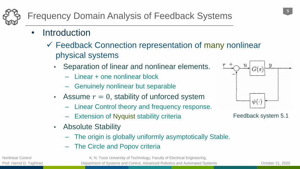
• Introduction
Feedback Connection representation of many nonlinear
physical systems
• Separation of linear and nonlinear elements.
– Linear + one nonlinear block
– Genuinely nonlinear but separable
• Assume 𝑟 = 0, stability of unforced system
– Linear Control theory and frequency response.
– Extension of Nyquist stability criteria
• Absolute Stability
– The origin is globally uniformly asymptotically Stable.
– The Circle and Popov criteria
Feedback system 5.1

Nonlinear Control K. N. Toosi University of Technology, Faculty of Electrical Engineering,
Prof. Hamid D. Taghirad Department of Systems and Control, Advanced Robotics and Automated Systems October 21, 2020
Frequency Domain Analysis of Feedback Systems6
• Absolute Stability
Consider the feedback connected system by closed-loop non-autonomous system
ሶ𝑥 = 𝐴𝑥 + 𝐵𝑢 (7.1)
𝑦 = 𝐶𝑥 + 𝐷𝑢 (7.2)
𝑢 = −𝜓(𝑡, 𝑦) (7.3)
• where (𝐴, 𝐵) is controllable, (𝐴, 𝐶) is observable,
• And 𝜓 is a memoryless, possibly time varying nonlinearity
– Piecewise continuous in 𝑡 and locally Lipschitz in 𝑦
• The transfer matrix of the system:
𝐺 𝑠 = 𝐶 𝑠𝐼 − 𝐴 −1𝐵 + 𝐷 (7.4)
• For all nonlinearities, origin is the eq. point.
• Lure’s problem: Study the stability for sector type nonlinearity.

Nonlinear Control K. N. Toosi University of Technology, Faculty of Electrical Engineering,
Prof. Hamid D. Taghirad Department of Systems and Control, Advanced Robotics and Automated Systems October 21, 2020
Absolute Stability7
• Definitions

Nonlinear Control K. N. Toosi University of Technology, Faculty of Electrical Engineering,
Prof. Hamid D. Taghirad Department of Systems and Control, Advanced Robotics and Automated Systems October 21, 2020
Absolute Stability8
• Definitions
Absolute Stability
• The stability is examined using two Ly. Functions
– Weighted norm Lyapunov function:
– Lure type Lyapunov function:
Nonlinear Control K. N. Toosi University of Technology, Faculty of Electrical Engineering,
Prof. Hamid D. Taghirad Department of Systems and Control, Advanced Robotics and Automated Systems October 21, 2020
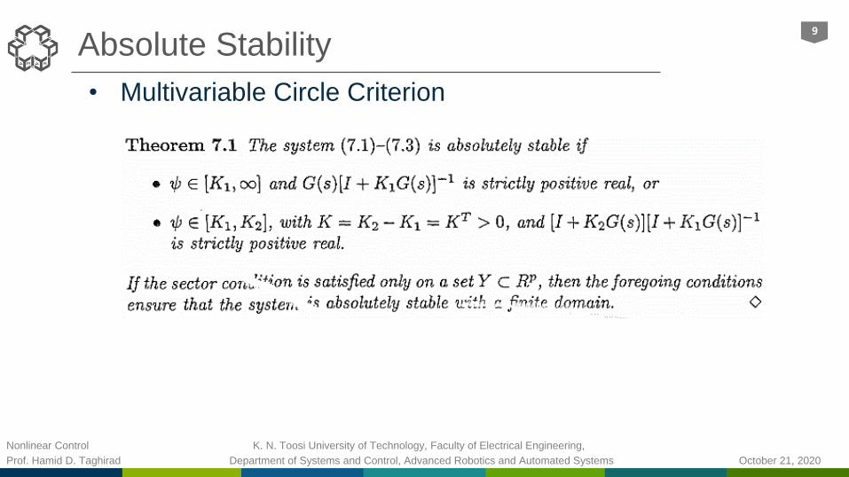
Absolute Stability9
• Multivariable Circle Criterion

Nonlinear Control K. N. Toosi University of Technology, Faculty of Electrical Engineering,
Prof. Hamid D. Taghirad Department of Systems and Control, Advanced Robotics and Automated Systems October 21, 2020
Absolute Stability10
• Circle Criterion:

Nonlinear Control K. N. Toosi University of Technology, Faculty of Electrical Engineering,
Prof. Hamid D. Taghirad Department of Systems and Control, Advanced Robotics and Automated Systems October 21, 2020
Absolute Stability11
• Circle Criterion:
Graphical Representation
• Disk 𝐷(𝛼 , 𝛽) is shown graphically
• Extension of Nyquist criteria by replacement of −1/𝑘 to the disk 𝐷(𝛼 , 𝛽).

Nonlinear Control K. N. Toosi University of Technology, Faculty of Electrical Engineering,
Prof. Hamid D. Taghirad Department of Systems and Control, Advanced Robotics and Automated Systems October 21, 2020
Absolute Stability12
• Circle Criterion:
Example 1: Consider the system
• Sector Nonlinearity [𝛼, 𝛽]
– Case (a): 𝛼 < 0 < 𝛽
– For absolute stability the Nyquist must lie inside circle:
– 1st choice:
𝐷(𝛼 , 𝛽) = [−1/4 ,+1/4] = [−0.25,+0.25]
• This is not the largest sector.
– 2nd choice: dotted circle:
– D(α ,β) = [-1/4.4 , +1/1.4]
= [-0.227, +0.714]
• Better than the 1st choice.
4-1.4

Nonlinear Control K. N. Toosi University of Technology, Faculty of Electrical Engineering,
Prof. Hamid D. Taghirad Department of Systems and Control, Advanced Robotics and Automated Systems October 21, 2020
Absolute Stability13
• Circle Criterion:
Example 1: (Cont.)
• Sector Nonlinearity [𝛼, 𝛽]
– Case (b): 0 = 𝛼 < 𝛽
– For absolute stability the Nyquist must lie to the right of line Re(s) -
0.875:
– 𝐷(𝛼 , 𝛽) = [0 ,+1/0.875]
= [0 , 1.117]
– This is not the largest sector.
-0.875

Nonlinear Control K. N. Toosi University of Technology, Faculty of Electrical Engineering,
Prof. Hamid D. Taghirad Department of Systems and Control, Advanced Robotics and Automated Systems October 21, 2020
Absolute Stability14
• Circle Criterion: Example 2: Consider the system
• Linear system + saturation
• Saturation lies in the sector [0 , 1]:
• According to Ex 1 case b, the system is absolutely stable.
Nonlinear Control K. N. Toosi University of Technology, Faculty of Electrical Engineering,
Prof. Hamid D. Taghirad Department of Systems and Control, Advanced Robotics and Automated Systems October 21, 2020
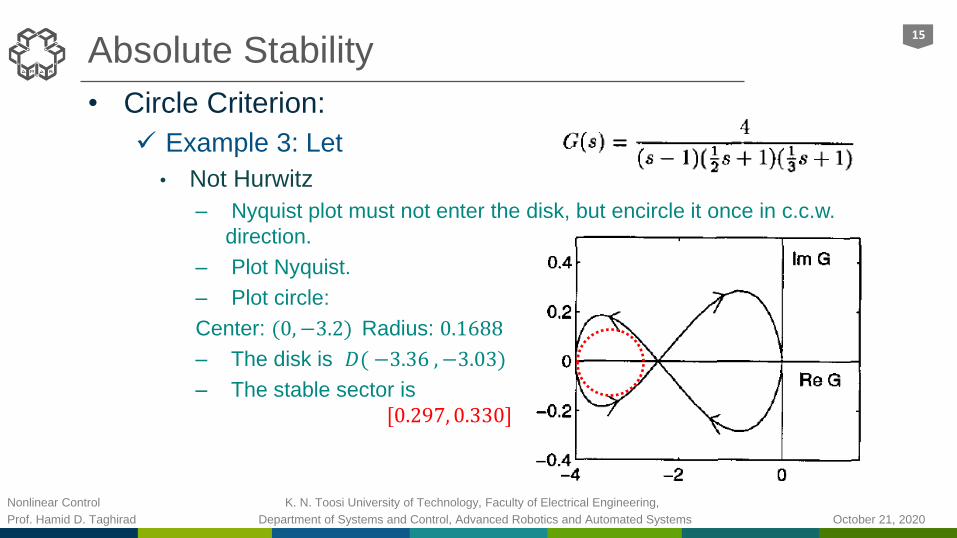
Absolute Stability15
• Circle Criterion:
Example 3: Let
• Not Hurwitz
– Nyquist plot must not enter the disk, but encircle it once in c.c.w.
direction.
– Plot Nyquist.
– Plot circle:
Center: (0,−3.2) Radius: 0.1688
– The disk is 𝐷( −3.36 ,−3.03)
– The stable sector is
[0.297, 0.330]

Nonlinear Control K. N. Toosi University of Technology, Faculty of Electrical Engineering,
Prof. Hamid D. Taghirad Department of Systems and Control, Advanced Robotics and Automated Systems October 21, 2020
Absolute Stability16
• Circle Criterion:
Example 4: Let
• Nonlinearity is saturation belonging to sector [0, 1]
– Not Hurwitz, Nyquist plot must not enter the
disk, but encircle it once in c.c.w. direction.
– Plot Nyquist, and the circle:
Center ∶ (0, −1),Radius ∶ 0.45
– The disk is 𝐷(−0.55,−1.45)
– The stable sector is [0.690, 1.818]
– The system is not globally asymptotically
stable, and it is only absolutely stable in a
finite domain.

Nonlinear Control K. N. Toosi University of Technology, Faculty of Electrical Engineering,
Prof. Hamid D. Taghirad Department of Systems and Control, Advanced Robotics and Automated Systems October 21, 2020
Absolute Stability17
• Popov Criteria:
Consider the feedback connected system by closed-loop non-autonomous system
ሶ𝑥 = 𝐴𝑥 + 𝐵𝑢 (7.13)
𝑦 = 𝐶𝑥 (7.14)
𝑢𝑖 = −𝜓𝑖 𝑦𝑖 , 1 ≤ 𝑖 ≤ 𝑝 (7.15)
• where (𝐴, 𝐵) is controllable, (𝐴, 𝐶) is observable,
• And 𝜓𝑖 is a memoryless nonlinearity belonging to sector [0, 𝑘𝑖]
• The transfer matrix of the system is strictly proper:
𝐺 𝑠 = 𝐶 𝑠𝐼 − 𝐴 −1𝐵
• With the Lure-type Lyapunov function absolute stability of the system is proved.

Nonlinear Control K. N. Toosi University of Technology, Faculty of Electrical Engineering,
Prof. Hamid D. Taghirad Department of Systems and Control, Advanced Robotics and Automated Systems October 21, 2020
Absolute Stability18
• Multivariable Popov Criteria:
• For 𝑀 + 𝐼 + 𝑠Γ 𝐺 𝑠 be strictly positive real 𝐺 𝑠 must be Hurwitz.
For scalar case the following theorem may be stated.

Nonlinear Control K. N. Toosi University of Technology, Faculty of Electrical Engineering,
Prof. Hamid D. Taghirad Department of Systems and Control, Advanced Robotics and Automated Systems October 21, 2020
Absolute Stability19
• Popov Criteria:
• Applicable only for SISO and stable systems.
• Only Sufficient Condition.
• Graphical representation of condition (7.19)
Theorem 7.4: Consider scalar nonlinearity 𝜙 and the feedback system (5.1) that satisfies the conditions:
• The matrix A is Hurwitz and the pair (A,B) is controllable.• The nonlinearity 𝜓 belongs to the sector [0, 𝑘]• There exists a positive number 𝛾 such that
Then the origin is globally asymptotically stable.

Nonlinear Control K. N. Toosi University of Technology, Faculty of Electrical Engineering,
Prof. Hamid D. Taghirad Department of Systems and Control, Advanced Robotics and Automated Systems October 21, 2020
Absolute Stability20
Popov Criteria:
Example: Consider the system
• Let 𝜓 = ℎ 𝑦 − 𝛼𝑦, 𝛼 > 0 to make the system matrix Hurwitz.
– Assume the sector nonlinearity ℎ ∈ 𝛼, 𝛽 , 𝛽 > 𝛼 > 0
– Then 𝜓 ∈ 0, 𝑘 , k = 𝛽 − 𝛼. Then, the Popov condition is
– For all positive values of 𝛼 and 𝑘 this is satisfied by 𝛾 > 1.

Nonlinear Control K. N. Toosi University of Technology, Faculty of Electrical Engineering,
Prof. Hamid D. Taghirad Department of Systems and Control, Advanced Robotics and Automated Systems October 21, 2020
Absolute Stability21
Popov Criteria:
Example: (Cont.)
– Even for 𝑘 = ∞, the popov condition is satisfied for all 𝜔
– Hence, the system is absolutely stable for all ℎ in the sector 𝛼,∞ ,
where 𝛼 can be arbitrary small.
– The Popov plot is shown for 𝛼 = 1.

Nonlinear Control K. N. Toosi University of Technology, Faculty of Electrical Engineering,
Prof. Hamid D. Taghirad Department of Systems and Control, Advanced Robotics and Automated Systems October 21, 2020
Contents
In this chapter we review absolute stability of a linear feedback system with a nonlinear block. Circle and Popov criterion in single variable, andmultivariable systems are described in detail. Then by quasi-linear approximation of nonlinear feedback systems into a linear and a nonlinear block, existence, stability and frequency and amplitude of limit cycles are analyzed, by using describing function analysis.
22
Absolute StabilityIntroduction, definitions, sector nonlinearity, Lure’s problem, Multivariable and single variable circle and Popov criteria.1
Describing Function MethodIllustrating example, assumptions and definitions, computing describing functions for common nonlinearities.2
Describing Function MethodReview of Nyquist criterion, Existence and stability of limit cycles, examples.3

Nonlinear Control K. N. Toosi University of Technology, Faculty of Electrical Engineering,
Prof. Hamid D. Taghirad Department of Systems and Control, Advanced Robotics and Automated Systems October 21, 2020
Frequency Domain Analysis of Feedback Systems23
• Describing Function Method
Illustrating Example: Van der Pol
• System Dynamics: ሷ𝑥 + 𝛼 𝑥2 − 1 ሶ𝑥 + 𝑥 = 0
• Assume, a disk type limit cycle 𝑥 𝑡 = 𝐴𝑠𝑖𝑛(𝜔𝑡)
– With amplitude 𝐴 and frequency 𝜔.
Separate the linear and nonlinear elements, and Integrate it into
feedback system (5.2)
ሷ𝑥 − 𝛼 ሶ𝑥 + 𝑥 = 𝛼(−𝑥2 ሶ𝑥)
– Consider the nonlinear term 𝑤 𝑥 = −𝑥2 ሶ𝑥 in the feedback.
𝐺(𝑠)𝑤(⋅)𝑥(𝑡)𝑤(𝑡)−𝑥(𝑡)𝑟 = 0
−+
Nonlinearity Linear SystemFeedback System 5.2

Nonlinear Control K. N. Toosi University of Technology, Faculty of Electrical Engineering,
Prof. Hamid D. Taghirad Department of Systems and Control, Advanced Robotics and Automated Systems October 21, 2020
Describing Function Method24
Illustrating Example: Van der Pol (Cont.)
• Then the linear system is
𝐺 𝑠 =𝑥
𝑢=
𝛼
𝑠2−𝛼 𝑠+1
• Approximate the nonlinear element
– For a limit cycle 𝑥 𝑡 ≈ 𝐴 sin(𝜔𝑡) ⇒ ሶ𝑥 = 𝐴𝜔 cos 𝜔𝑡
𝑤 = −𝑥2 ሶ𝑥 = −𝐴2 sin2(𝜔𝑡) 𝐴𝜔 cos 𝜔𝑡
=−1
2𝐴3𝜔 1 − cos 2𝜔𝑡 cos 𝜔𝑡 =
−1
4𝐴3𝜔 cos(𝜔𝑡) − cos(3𝜔𝑡)
• Approximate the output
𝑤 ≈−𝐴3
4𝜔 cos 𝜔𝑡 =
𝐴2
4
𝑑
𝑑𝑡−𝐴 sin 𝜔𝑡 =
𝐴2
4(−𝑠𝑥)
• Input/Output Quasi-Linear approximation
𝑤
𝑥≈𝐴2
4−𝑠
– Amplitude dependent

Nonlinear Control K. N. Toosi University of Technology, Faculty of Electrical Engineering,
Prof. Hamid D. Taghirad Department of Systems and Control, Advanced Robotics and Automated Systems October 21, 2020
Describing Function Method25
Quasi-linear block diagram
• The frequency response estimate:
𝑤 = 𝑁 𝐴,𝜔 −𝑥 ⇒ 𝑁 𝐴,𝜔 =𝐴2
4𝑗𝜔
• Existence of limit cycle: ∃ 𝑥 𝑡 ≈ 𝐴 sin 𝜔𝑡 , ∋
𝑥 𝑡 ≈ 𝐴 sin 𝜔𝑡 = 𝐺 𝑗𝜔 𝑁(𝐴, 𝜔)(−𝑥) ⇒ 1 + 𝐺 𝑗𝜔 𝑁 𝐴,𝜔 𝑥
– For a nontrivial limit cycle: 𝑥 𝑡 ≠ 0 → 1 + 𝐺 𝑗𝜔 𝑁 𝐴,𝜔 = 0
– Compare Nyquist criteria: 1 + 𝐺 𝑗𝜔 ⋅ 𝑘 = 0
𝛼
𝑠2 − 𝛼𝑠 + 1
𝑥(𝑡)𝑤(𝑡)−𝑥(𝑡)𝑟 = 0
−+
𝐴2
4𝑝
Quasi-linear Approximation 𝐺(𝑠)

Nonlinear Control K. N. Toosi University of Technology, Faculty of Electrical Engineering,
Prof. Hamid D. Taghirad Department of Systems and Control, Advanced Robotics and Automated Systems October 21, 2020
Describing Function Method26
Illustrating Example: Van der Pol (Cont.)
• Graphical Solution
– Intersect 𝐺(𝑗𝜔) and −1/𝑁(𝐴,𝜔)
• Analytical Solution (for 𝑝 = 𝑗𝜔)
2( )
1G j
j
2 2
1 4 4
( , )
j
N A A j A
2
4, 1 2
jj A
A
𝜔 = 1
𝐺(𝑗𝜔)
−1/𝑁(𝐴,𝜔)
1,2p
2
2 2 2
4 0 2
11 1/ 64 ( 4)
A A
A

Nonlinear Control K. N. Toosi University of Technology, Faculty of Electrical Engineering,
Prof. Hamid D. Taghirad Department of Systems and Control, Advanced Robotics and Automated Systems October 21, 2020
Describing Function Method
Illustrating Example: Van der Pol (Cont.)
• Graphical Solution
The approx. limit cycle
parameters does not
depend on 𝛼
𝜔 = 1
−1/𝑁(𝐴, 𝜔)
𝐺(𝑗𝜔), 𝛼 = 2
𝐺(𝑗𝜔), 𝛼 = 1
𝐺(𝑗𝜔), 𝛼 = 4
Nonlinear Control K. N. Toosi University of Technology, Faculty of Electrical Engineering,
Prof. Hamid D. Taghirad Department of Systems and Control, Advanced Robotics and Automated Systems October 21, 2020
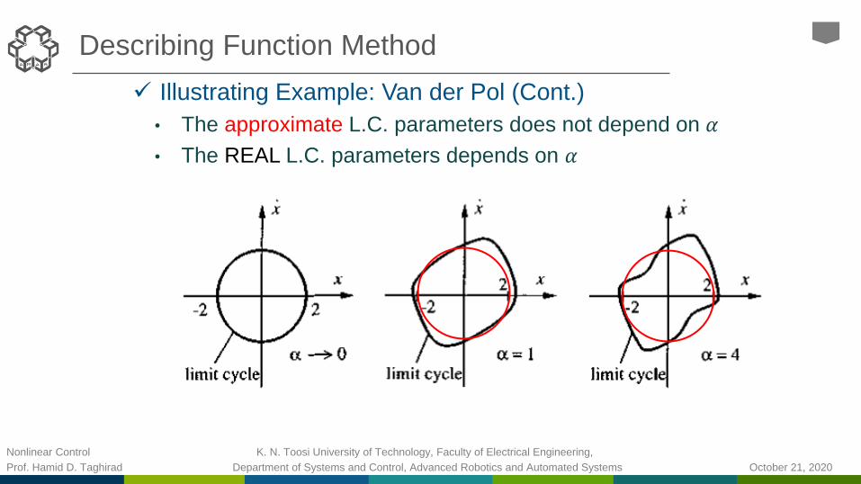
Describing Function Method
Illustrating Example: Van der Pol (Cont.)
• The approximate L.C. parameters does not depend on 𝛼
• The REAL L.C. parameters depends on 𝛼
Nonlinear Control K. N. Toosi University of Technology, Faculty of Electrical Engineering,
Prof. Hamid D. Taghirad Department of Systems and Control, Advanced Robotics and Automated Systems October 21, 2020
Describing Function Method29
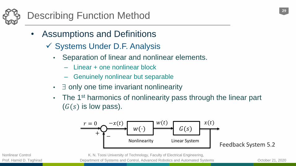
• Assumptions and Definitions
Systems Under D.F. Analysis
• Separation of linear and nonlinear elements.
– Linear + one nonlinear block
– Genuinely nonlinear but separable
• only one time invariant nonlinearity
• The 1st harmonics of nonlinearity pass through the linear part
(𝐺(𝑠) is low pass).
𝐺(𝑠)𝑤(⋅)𝑥(𝑡)𝑤(𝑡)−𝑥(𝑡)𝑟 = 0
−+
Nonlinearity Linear SystemFeedback System 5.2

Nonlinear Control K. N. Toosi University of Technology, Faculty of Electrical Engineering,
Prof. Hamid D. Taghirad Department of Systems and Control, Advanced Robotics and Automated Systems October 21, 2020
Describing Function Method30
• Assumptions and Definitions
Nonlinear function
• For a Limit cycle the output is periodic.
• Use Fourier Series to represent the output.
• For odd nonlinearities 𝑎0 = 0.
• By 3rd assumption consider just the first harmonics.

Nonlinear Control K. N. Toosi University of Technology, Faculty of Electrical Engineering,
Prof. Hamid D. Taghirad Department of Systems and Control, Advanced Robotics and Automated Systems October 21, 2020
Describing Function Method31
• Assumptions and Definitions
Nonlinear function (cont.)
– In which
– In complex representation
• Describing Function
– Extension of input/output transfer function:

Nonlinear Control K. N. Toosi University of Technology, Faculty of Electrical Engineering,
Prof. Hamid D. Taghirad Department of Systems and Control, Advanced Robotics and Automated Systems October 21, 2020
Describing Function Method32
• Computing Describing Functions
Common nonlinearities
• Hardening Spring
– Fourier series for input: :
– Nonlinearity is odd: 𝑎0 = 𝑎1 = 0, and
– Therefore,
– Describing Function is:
– Note: D.F. is real and does not depend on 𝜔
Nonlinear Control K. N. Toosi University of Technology, Faculty of Electrical Engineering,
Prof. Hamid D. Taghirad Department of Systems and Control, Advanced Robotics and Automated Systems October 21, 2020
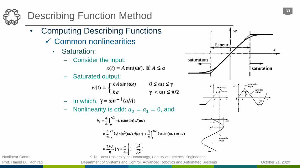
Describing Function Method33
• Computing Describing Functions
Common nonlinearities
• Saturation:
– Consider the input:
– Saturated output:
– In which,
– Nonlinearity is odd: 𝑎0 = 𝑎1 = 0, and
Nonlinear Control K. N. Toosi University of Technology, Faculty of Electrical Engineering,
Prof. Hamid D. Taghirad Department of Systems and Control, Advanced Robotics and Automated Systems October 21, 2020
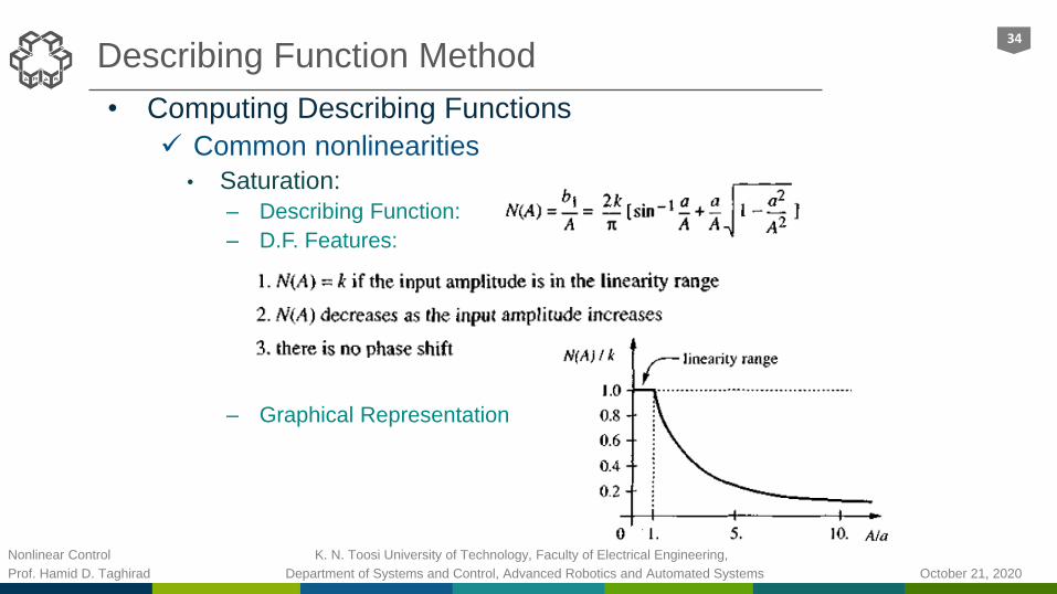
Describing Function Method34
• Computing Describing Functions
Common nonlinearities
• Saturation:
– Describing Function:
– D.F. Features:
– Graphical Representation

Nonlinear Control K. N. Toosi University of Technology, Faculty of Electrical Engineering,
Prof. Hamid D. Taghirad Department of Systems and Control, Advanced Robotics and Automated Systems October 21, 2020
Describing Function Method35
• Computing Describing Functions
Common nonlinearities
• Relay: Special case of saturation
– Direct determination:
– Describing Function:
Nonlinear Control K. N. Toosi University of Technology, Faculty of Electrical Engineering,
Prof. Hamid D. Taghirad Department of Systems and Control, Advanced Robotics and Automated Systems October 21, 2020
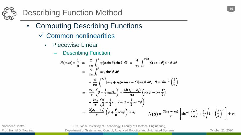
Describing Function Method36
• Computing Describing Functions
Common nonlinearities
• Piecewise Linear
– Describing Function
1( , )b
N aa
( )N a

Nonlinear Control K. N. Toosi University of Technology, Faculty of Electrical Engineering,
Prof. Hamid D. Taghirad Department of Systems and Control, Advanced Robotics and Automated Systems October 21, 2020
Describing Function Method37
• Computing Describing Functions
Common nonlinearities
• Piecewise Linear
– Describing Function: Graphical Representation
• Saturation
– Special case of piecewise linear with

Nonlinear Control K. N. Toosi University of Technology, Faculty of Electrical Engineering,
Prof. Hamid D. Taghirad Department of Systems and Control, Advanced Robotics and Automated Systems October 21, 2020
Describing Function Method38
• Computing Describing Functions
Common nonlinearities
• Dead-Zone
– Nonlinear function
– In which,
– Nonlinearity is odd: 𝑎0 = 𝑎1 = 0, and

Nonlinear Control K. N. Toosi University of Technology, Faculty of Electrical Engineering,
Prof. Hamid D. Taghirad Department of Systems and Control, Advanced Robotics and Automated Systems October 21, 2020
Describing Function Method39
• Computing Describing Functions
Common nonlinearities
• Dead-Zone
– Describing Function
– Real, A dependent
– Not depending on 𝜔
– No phase shift
– Graphical
Representation

Nonlinear Control K. N. Toosi University of Technology, Faculty of Electrical Engineering,
Prof. Hamid D. Taghirad Department of Systems and Control, Advanced Robotics and Automated Systems October 21, 2020
Describing Function Method40
• Computing Describing Functions
Common nonlinearities
• Backlash
Nonlinear Control K. N. Toosi University of Technology, Faculty of Electrical Engineering,
Prof. Hamid D. Taghirad Department of Systems and Control, Advanced Robotics and Automated Systems October 21, 2020
Describing Function Method41
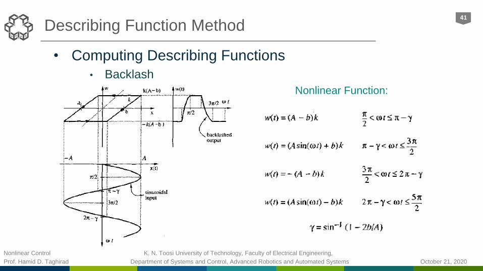
• Computing Describing Functions
• Backlash
Nonlinear Function:
In which

Nonlinear Control K. N. Toosi University of Technology, Faculty of Electrical Engineering,
Prof. Hamid D. Taghirad Department of Systems and Control, Advanced Robotics and Automated Systems October 21, 2020
Describing Function Method42
• Computing Describing Functions
• Backlash
– Describing Function:
– Therefore,
– D.F. Graphical Representation

Nonlinear Control K. N. Toosi University of Technology, Faculty of Electrical Engineering,
Prof. Hamid D. Taghirad Department of Systems and Control, Advanced Robotics and Automated Systems October 21, 2020
Contents
In this chapter we review absolute stability of a linear feedback system with a nonlinear block. Circle and Popov criterion in single variable, andmultivariable systems are described in detail. Then by quasi-linear approximation of nonlinear feedback systems into a linear and a nonlinear block, existence, stability and frequency and amplitude of limit cycles are analyzed, by using describing function analysis.
43
Absolute StabilityIntroduction, definitions, sector nonlinearity, Lure’s problem, Multivariable and single variable circle and Popov criteria.1
Describing Function MethodIllustrating example, assumptions and definitions, computing describing functions for common nonlinearities.2
Describing Function AnalysisReview of Nyquist criterion, Existence and stability of limit cycles, examples.3

Nonlinear Control K. N. Toosi University of Technology, Faculty of Electrical Engineering,
Prof. Hamid D. Taghirad Department of Systems and Control, Advanced Robotics and Automated Systems October 21, 2020
Describing Function Method44
• Review of Nyquist Criterion
Feedback system
• Loop gain 𝐿(𝑠) = 𝐶(𝑠)𝑃(𝑠)
– Characteristic Equation 1 + 𝐿(𝑠) = 0 or 𝐿(𝑠) = −1
– Draw the Nyquist plot of 𝐿(𝑗𝜔) for − < 𝜔 < +
– Count the number of c.w. encirclement of the Nyquist plot around point (−1,0). 𝑁
– Compute the number of unstable poles of the loop gain 𝐿(𝑠). 𝑃
– The number of unstable roots of the characteristic equation (or the number of unstable poles of the closed-loop transfer function) is denoted by 𝑍 and is found from: 𝑍 = 𝑁 + 𝑃
𝑃(𝑠)𝐶(𝑠)+ -

Nonlinear Control K. N. Toosi University of Technology, Faculty of Electrical Engineering,
Prof. Hamid D. Taghirad Department of Systems and Control, Advanced Robotics and Automated Systems October 21, 2020
Describing Function Analysis45
• Review of Nyquist Criterion
Feedback system
• Loop gain 𝐿(𝑠) = 𝐶(𝑠)𝑃(𝑠)
– Characteristic Equation 1 + 𝑘 𝐿(𝑠) = 0 or 𝐿(𝑠) = −1 / 𝑘
– Draw the Nyquist plot of 𝐿(𝑗𝜔) for − < 𝜔 < +
– Count the number of c.w. encirclement of the Nyquist plot around
point (−1 / 𝑘 , 0). 𝑁
– Compute the number of unstable poles of the loop gain 𝐿(𝑠). 𝑃
– The number of unstable roots of the characteristic equation (or the number of unstable poles of the closed-loop transfer function) is denoted by 𝑍 and is found from: 𝑍 = 𝑁 + 𝑃
𝐿(𝑠)𝑘+
-

Nonlinear Control K. N. Toosi University of Technology, Faculty of Electrical Engineering,
Prof. Hamid D. Taghirad Department of Systems and Control, Advanced Robotics and Automated Systems October 21, 2020
Describing Function Analysis46
• Existence of Limit Cycle
Feedback System𝑥 = −𝑦
𝑤 = 𝑁 𝐴,𝜔 𝑥𝑦 = 𝐺 𝑗𝜔 𝑤
⇒ 𝑦 = 𝐺 𝑗𝜔 𝑁 𝐴,𝜔 (−𝑦)
• Characteristics Equation: (for 𝑦 0 )
𝐺 𝑗𝜔 𝑁 𝐴,𝜔 + 1 = 0 OR 𝐺 𝑗𝜔 = −1
𝑁 𝐴,𝜔
• Solve it Graphically
• Amplitude dependent describing function
– Intersect 𝐺(𝑗𝜔) and −1/𝑁(𝐴)
– If intersection occurs L.C. exists
– Amplitude of L.C. 𝐴 (on −1/𝑁(𝐴))
– Frequency of L.C. 𝜔 (on 𝐺(𝑗𝜔))

Nonlinear Control K. N. Toosi University of Technology, Faculty of Electrical Engineering,
Prof. Hamid D. Taghirad Department of Systems and Control, Advanced Robotics and Automated Systems October 21, 2020
Describing Function Analysis47
• Existence of Limit Cycle
Graphical Solution
• General Describing Function (𝑁(𝐴,𝜔))
– Plot 𝐺(𝑗𝜔)
– Plot a set of −1/𝑁(𝐴,𝜔) for different constant frequencies.
– Analyze the intersection points
– If an intersection point in which
The frequencies match L.C. exists
– Amplitude of L.C. 𝐴 (on -1/𝑁(𝐴,𝜔))
– Frequency of L.C. the matched 𝜔
(on 𝐺(𝑗𝜔) and on -1/𝑁(𝐴,𝜔))

Nonlinear Control K. N. Toosi University of Technology, Faculty of Electrical Engineering,
Prof. Hamid D. Taghirad Department of Systems and Control, Advanced Robotics and Automated Systems October 21, 2020
Describing Function Analysis48
• Stability of Limit Cycle
Feedback System
• Characteristics Equation: (for 𝑦 0 )
𝐺 𝑗𝜔 𝑁 𝐴,𝜔 + 1 = 0 OR 𝐺 𝑗𝜔 = −1
𝑁 𝐴,𝜔
Compare it with Nyquist criteria:
𝐿 𝑠 𝑘 + 1 = 0 or 𝐿(𝑠) = −1 / 𝑘
• Extended Nyquist Criteria
– Replace the point −1/𝑘 by −1/𝑁(𝐴,𝜔) and count encirclements
– Apply the same Nyquist criteria to determine stability
– Note: stability decay of amplitude
– Instability increase of amplitude
Nonlinear Control K. N. Toosi University of Technology, Faculty of Electrical Engineering,
Prof. Hamid D. Taghirad Department of Systems and Control, Advanced Robotics and Automated Systems October 21, 2020
Unstable Region
Describing Function Analysis49
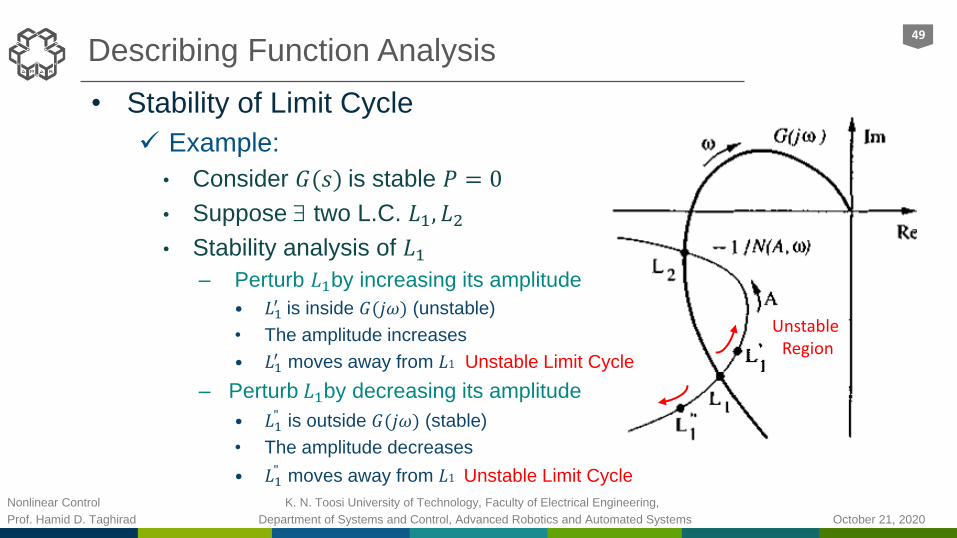
• Stability of Limit Cycle
Example:
• Consider 𝐺(𝑠) is stable 𝑃 = 0
• Suppose two L.C. 𝐿1, 𝐿2• Stability analysis of 𝐿1
– Perturb 𝐿1by increasing its amplitude
• 𝐿1′ is inside 𝐺(𝑗𝜔) (unstable)
• The amplitude increases
• 𝐿1′ moves away from 𝐿1 Unstable Limit Cycle
– Perturb 𝐿1by decreasing its amplitude
• 𝐿1" is outside 𝐺(𝑗𝜔) (stable)
• The amplitude decreases
• 𝐿1" moves away from 𝐿1 Unstable Limit Cycle
Nonlinear Control K. N. Toosi University of Technology, Faculty of Electrical Engineering,
Prof. Hamid D. Taghirad Department of Systems and Control, Advanced Robotics and Automated Systems October 21, 2020
Describing Function Analysis50
'
2L
"
2L
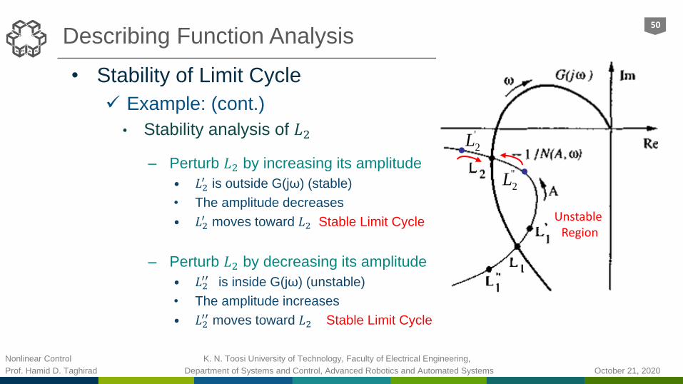
• Stability of Limit Cycle
Example: (cont.)
• Stability analysis of 𝐿2
– Perturb 𝐿2 by increasing its amplitude
• 𝐿2′ is outside G(jω) (stable)
• The amplitude decreases
• 𝐿2′ moves toward 𝐿2 Stable Limit Cycle
– Perturb 𝐿2 by decreasing its amplitude
• 𝐿2′′ is inside G(jω) (unstable)
• The amplitude increases
• 𝐿2′′ moves toward 𝐿2 Stable Limit Cycle
Unstable Region

Nonlinear Control K. N. Toosi University of Technology, Faculty of Electrical Engineering,
Prof. Hamid D. Taghirad Department of Systems and Control, Advanced Robotics and Automated Systems October 21, 2020
• Example 1:
Consider 𝐺 𝑠 =1
𝑠(𝑠+1)(𝑠+2)with unit
• Nyquist Plot
𝐺 𝑗𝜔 = −3𝜔 − 𝑗(2 − 𝜔2)
9𝜔3 + 𝜔 2 − 𝜔2 2
– @ point A
ℑ 𝐺 𝑗𝜔 = 0 → 2 − 𝜔2 = 0 → 𝜔 = 2
𝐴 = 𝐺 𝑗 2 = −3 2
18 2 + 0= −
1
6
(a) For unit saturation (𝑘 = 1)
– 𝑁(𝐴) < 1 No Crossing, No Limit Cycle
Describing Function Analysis51
a) Saturation
b) Relay
−1/𝑁(𝐴)
𝐺(𝑗𝜔)

Nonlinear Control K. N. Toosi University of Technology, Faculty of Electrical Engineering,
Prof. Hamid D. Taghirad Department of Systems and Control, Advanced Robotics and Automated Systems October 21, 2020
• Example 1: (Cont.)
(b) For unit Relay (M=1)
– − < −1/𝑁(𝐴) < 0 Crossing @ point A
– Amplitude:−1
𝑁 𝐴= −
1
6→
𝑁 𝐴 =4
𝜋𝐴= 6 → 𝐴 =
2
3𝜋
– Frequency: 𝜔 = 2 and Limit Cycle is stable.
Describing Function Analysis52
−1/𝑁(𝐴)
𝐺(𝑗𝜔)
Unstable Region
𝐴
𝐿′
Nonlinear Control K. N. Toosi University of Technology, Faculty of Electrical Engineering,
Prof. Hamid D. Taghirad Department of Systems and Control, Advanced Robotics and Automated Systems October 21, 2020
Describing Function Analysis53
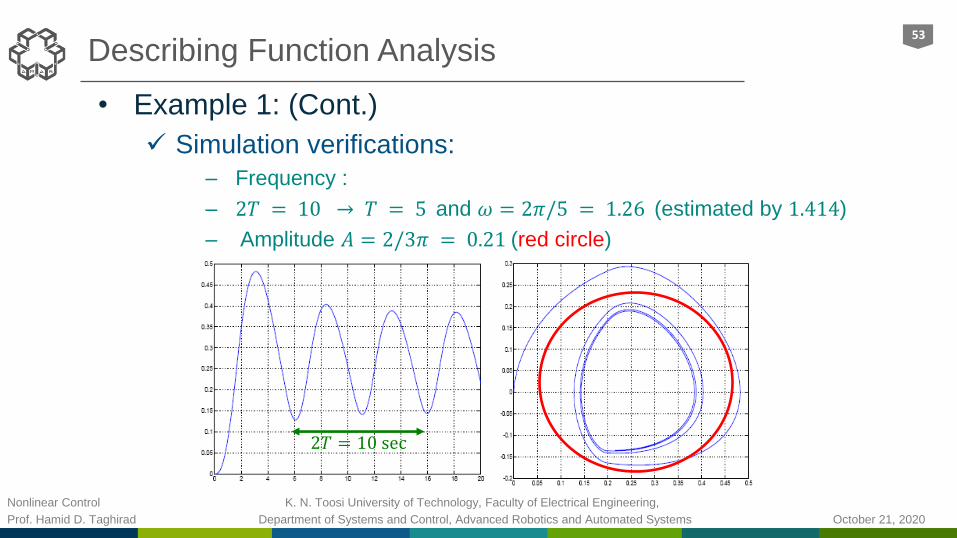
• Example 1: (Cont.)
Simulation verifications:
– Frequency :
– 2𝑇 = 10 → 𝑇 = 5 and 𝜔 = 2𝜋/5 = 1.26 (estimated by 1.414)
– Amplitude 𝐴 = 2/3𝜋 = 0.21 (red circle)
2𝑇 = 10 sec

Nonlinear Control K. N. Toosi University of Technology, Faculty of Electrical Engineering,
Prof. Hamid D. Taghirad Department of Systems and Control, Advanced Robotics and Automated Systems October 21, 2020
Describing Function Analysis54
• Example 2:
Consider 𝐺 𝑠 =−𝑠
𝑠2+0.8𝑠+8with
• Nyquist Plot
– @ point A
(a) For unit saturation (𝑘 = 1)
– −1
𝑁 𝐴= −1.25 → 𝑁 𝐴 = 0.8
– 𝐴 1.455 @ 𝜔 = 2.83 Stable Limit Cycle
a) Saturation, 1, 1
b) Dead-zone, 1, 0.5
k a
k
2 2
2 2 2
0.8 (8 )( )
0.64 (8 )
jG j
2( ( )) 0 (8 ) 0 2 2G j
( 2) 1.25A G j
−1/𝑁(𝐴)
𝐺(𝑗𝜔)
−1 Unstable Region
Nonlinear Control K. N. Toosi University of Technology, Faculty of Electrical Engineering,
Prof. Hamid D. Taghirad Department of Systems and Control, Advanced Robotics and Automated Systems October 21, 2020
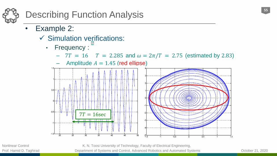
Describing Function Analysis55
• Example 2:
Simulation verifications:
• Frequency :
– 7𝑇 = 16 𝑇 = 2.285 and 𝜔 = 2𝜋/𝑇 = 2.75 (estimated by 2.83)
– Amplitude 𝐴 = 1.45 (red ellipse)
7𝑇 = 16sec

Nonlinear Control K. N. Toosi University of Technology, Faculty of Electrical Engineering,
Prof. Hamid D. Taghirad Department of Systems and Control, Advanced Robotics and Automated Systems October 21, 2020
56
Describing Function Analysis
• Example 2: (Cont.)
• (b) For Dead-zone 𝛿 = 1, 𝑘 = 0.5
• 0 < 𝑁 𝐴 < 0.5 𝑁 𝐴 0.8
• No Crossing No Limit Cycle
−2−1/𝑁(𝐴)
𝐺(𝑗𝜔)

Nonlinear Control K. N. Toosi University of Technology, Faculty of Electrical Engineering,
Prof. Hamid D. Taghirad Department of Systems and Control, Advanced Robotics and Automated Systems October 21, 2020
57
Describing Function Analysis
• Example 3:
Consider Raleigh’s Equation ሷ𝑥 + 𝑥 = 𝜖( ሶ𝑥 −1
3ሶ𝑥3)
• Separation ሷ𝑥 − 𝜖 ሶ𝑥 + 𝑥 = −𝜖(1
3ሶ𝑥3)
– Consider 𝑦 = ሶ𝑥 and 𝜙 𝑦 =1
3𝑦3
– 𝑠2 − 𝜖𝑠 + 1 𝑥 = −𝜖𝜙 𝑦 = −𝜖𝜙 𝑠𝑥 = −𝜖𝑠𝜙 𝑥
– Hence,
• Linear element: 𝐺 𝑠 =𝑥
𝜙=
𝜖𝑠
𝑠2−𝜖𝑠+1
• Nonlinear function: 𝜙 𝑦 =1
3𝑦3
𝐺(𝑠)𝜙(⋅)𝑥(𝑡)𝜙(𝑡)−𝑥(𝑡)𝑟 = 0
−+
Nonlinearity Linear System

Nonlinear Control K. N. Toosi University of Technology, Faculty of Electrical Engineering,
Prof. Hamid D. Taghirad Department of Systems and Control, Advanced Robotics and Automated Systems October 21, 2020
58
Describing Function Analysis
• Example 3:
Raleigh’s Equation (Cont.)
• Describing Function 𝜙 𝑦 =1
3𝑦3
• 𝑁 𝐴 =𝑏1
𝐴=
2
3𝜋A0𝜋𝐴 sin 𝜃 3 sin 𝜃 𝑑𝜃 =
1
4𝐴2
• Nyquist Plot
𝐺 𝑠 =𝜖𝑠
𝑠2 − 𝜖𝑠 + 1→ 𝐺 𝑗𝜔 =
𝜖𝑗𝜔 1 − 𝜔2 + 𝜖𝑗𝜔
1 − 𝜔2 2 + 𝜖2𝜔2
– @ point A
ℑ 𝐺 𝑗𝜔 = 0 → 1 − 𝜔2 = 0 → 𝜔 = 1
– 𝐴 = 𝐺 𝑗1 = −𝜖2
𝜖2= −1
– Regardless of 𝜖
𝐴

Nonlinear Control K. N. Toosi University of Technology, Faculty of Electrical Engineering,
Prof. Hamid D. Taghirad Department of Systems and Control, Advanced Robotics and Automated Systems October 21, 2020
59
Describing Function Analysis
• Example 3:
Raleigh’s Equation (Cont.)
• Intersect −1 / 𝑁(𝐴) with −1
• 𝑁 𝐴 =1
4𝐴2 = 1 → 𝐴 = 2
• A Limit cycle with
– Amplitude = 2
– Frequency = 1
• Stability analysis
– G(s) is unstable 𝑃 = 2
– For stable region 𝑁 = −2
– direction of −1/𝑁(𝑎)
• The limit cycle is STABLE
-40
-30
-20
-10
0
Magnitu
de (
dB
)
10-1
100
101
-270
-225
-180
-135
-90
Phase (
deg)
Bode Diagram
Frequency (rad/sec)
−1/𝑁(𝐴)
−1
N=-2: Stable Region

Nonlinear Control K. N. Toosi University of Technology, Faculty of Electrical Engineering,
Prof. Hamid D. Taghirad Department of Systems and Control, Advanced Robotics and Automated Systems October 21, 2020
60
Describing Function Analysis
• Example 3: Raleigh’s Equation (Cont.)
Simulation verifications:• Frequency :
– 2𝑇 = 13.34 𝜔 = 2𝜋/6.67 = 0.95 (estimated by 1)
– Amplitude 𝐴 = 2/3𝜋 = 0.21 (red circle)
𝟐𝑻 = 𝟏𝟑. 𝟑𝟒 𝒔𝒆𝒄

Nonlinear Control K. N. Toosi University of Technology, Faculty of Electrical Engineering,
Prof. Hamid D. Taghirad Department of Systems and Control, Advanced Robotics and Automated Systems October 21, 2020
Chapter 5: Frequency Domain Analysis of Feedback Systems
To read more and see the course videos visit our course website:
http://aras.kntu.ac.ir/arascourses/nonlinear-control/
Thank You
Nonlinear Control

Nonlinear Control K. N. Toosi University of Technology, Faculty of Electrical Engineering,
Prof. Hamid D. Taghirad Department of Systems and Control, Advanced Robotics and Automated Systems October 21, 2020
Hamid D. Taghirad has received his B.Sc. degree in mechanical engineering
from Sharif University of Technology, Tehran, Iran, in 1989, his M.Sc. in mechanical
engineering in 1993, and his Ph.D. in electrical engineering in 1997, both
from McGill University, Montreal, Canada. He is currently the University Vice-
Chancellor for Global strategies and International Affairs, Professor and the Director
of the Advanced Robotics and Automated System (ARAS), Department of Systems
and Control, Faculty of Electrical Engineering, K. N. Toosi University of Technology,
Tehran, Iran. He is a senior member of IEEE, and Editorial board of International
Journal of Robotics: Theory and Application, and International Journal of Advanced
Robotic Systems. His research interest is robust and nonlinear control applied to
robotic systems. His publications include five books, and more than 250 papers in
international Journals and conference proceedings.
About Hamid D. Taghirad
Hamid D. TaghiradProfessor