chapter 5 improving on time, in full...
TRANSCRIPT
70
CHAPTER 5
IMPROVING ON TIME, IN FULL DELIVERY
5.1 INTRODUCTION
The orders which are not yet shipped or invoiced to customer are
called backlog orders. The various reasons for accumulation of stock, i.e.
causes for slow moving inventory have been identified in the previous
chapter. This chapter focuses on finding ways to reduce the backlog orders
and/ or the slow moving inventory. The inventory meant here is the Board of
various sizes for different customers. The industry procures material as per
the customer sales order projection. Due to various reasons, the industry can’t
achieve more than 95% On Time In Full (OTIF) and hence the customer’s
production gets disturbed a lot. Hence, this chapter focuses on different ways
by which the OTIF can be improved in the printing and packaging industry by
means of various tools and methods like traceability, data warehouse, ANN
and Runge-Kutta method.
5.2 TRACKING AND IMPROVING THE ORDER FULFILMENT
PROCESS
5.2.1 Study of the Present System in the Industry
The entire supply chain management of the company has been
analyzed and found some constraints where some actions can be done to
improve the OTIF. In the existing system in industry in processing sale order,
customer sends the purchase order through mail, courier and fax to the
marketing department. The marketing department raises the sale order and
gives the customer requirement to every department and Product Introduction

71
Customer-
Purchase
order
Material-purchase order
request
Board division-
manufacturing
Sales
order
confirm/
print plan
ok
Slow moving
inventory
plan
Dispatch
Production department–production request
Marketing-raises thesales order
No
Yes
Mut
Process (PIP) Generates the Bill of Material (BOM) and as per that order the
materials department procures the material from the supplier and sends it to
company manufacturing division to manufacture as per the customer
specification. After the confirmation from the Customer, production
department checks for the print plan in the available Board and completes its
production and sends the material for dispatch. This is illustrated in
Figure 5.1.
Figure 5. 1 Order fulfillment processing flow chart

72
In this process, it is observed that there is a long time gap between
purchase order (PO) date and sale order (SO) date which leads to increase in
lead time. Ten orders has been taken to calculate its average time gap between
SO date and PO date. An average of five days is the time gap as shown in
Table 5.1, which is very high; so it is suggested to the company to reduce the
time gap between PO date and SO date.
5.2.2 Recommendation for improving order processing
It is recommended that sale order should be raised within 24 hrs of
receipt of purchase order. This can be done by the marketing team. The
marketing team should have regular contact with the customer so that they
can get the purchase order and raise the sale order immediately.
Table 5.1 Time gap between PO and SO
Sl.No. Purchase order date Sale order dateDifference (PO-SO)
days
1. 5-Jan-09 12-Jan-09 7
2. 2-Jan-09 8-Jan-09 6
3. 27-Jan-09 30-Jan-09 3
4. 2-Feb-09 6-Feb-09 4
5. 4-Feb-09 9-Feb-09 5
6. 10-Feb-09 15-Feb-09 5
7. 3-Dec-08 8-Dec-08 5
8. 12-Dec-08 16-Dec-08 4
9. 26-Dec-08 31-Dec-08 5
10. 31-Dec-08 6-Jan-09 6
Average 5 days

73
After implementing the above suggestion, the lead time was reduced
from 20 days to 16 days causing gradual increase in OTIF delivery.
5.3 TRACEABILITY FOR WAREHOUSE INVENTORY
Traceability is the ability to follow or study out in detail a step-by-
step history of certain activity or a process. The change in global economy has
significantly redefined the way enterprises are operated. In warehouse,
accurate monitoring and measurement of resources can be derived only from
timely and quality information, which many lack currently.
Hence, in this research an RFID based warehouse management
system is designed and proposed for the printing and packaging industry.
Planning and control of warehouse facilities system is more complex. RFID
resource management makes it easy to detect the material in the warehouse
and timely delivery to the production area by using real time data of RFID
tags to solve the picking up of correct material and information and location
of the material.
5.3.1 Current Status of the warehouse
Normally in present situation, it is increasingly difficult in locating
the material, even though they have an entry and a record. The data of
material and the amount that has been lost, for an industry of considerable
reputation in Chennai, due to inadequate traceability, during the past six
months (Sep 2007 to period ending Feb 2008) is shown in Table 5.2 and also
in bar chart Figure 5.2.
74
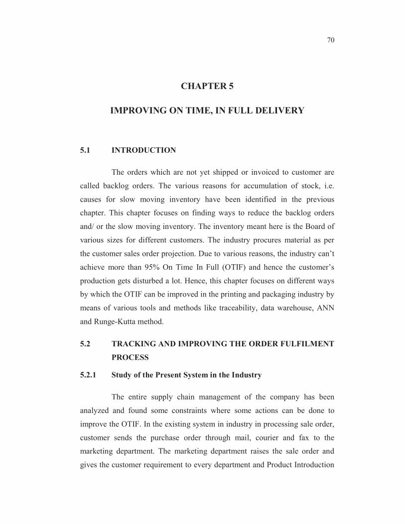
Table 5.2 The Data for non - traceable items in Warehouse
S.NoNot traceable
Items
Material
quantity
(Tons)
Material
cost (Rs)
Warehouse
cost (Rs)
Total cost
(Rs)
1 Film 47 705,000 16,309 721,309
2 Board 43 806,500 18,309 824,809
3 Inks 0.5 200,000 6,600 206,600
4 Glues 0.8 60,000 3,000 63,000
Total 1,771,500 44,218 1,815,718
Figure 5.2 Material cost for non-traceable items
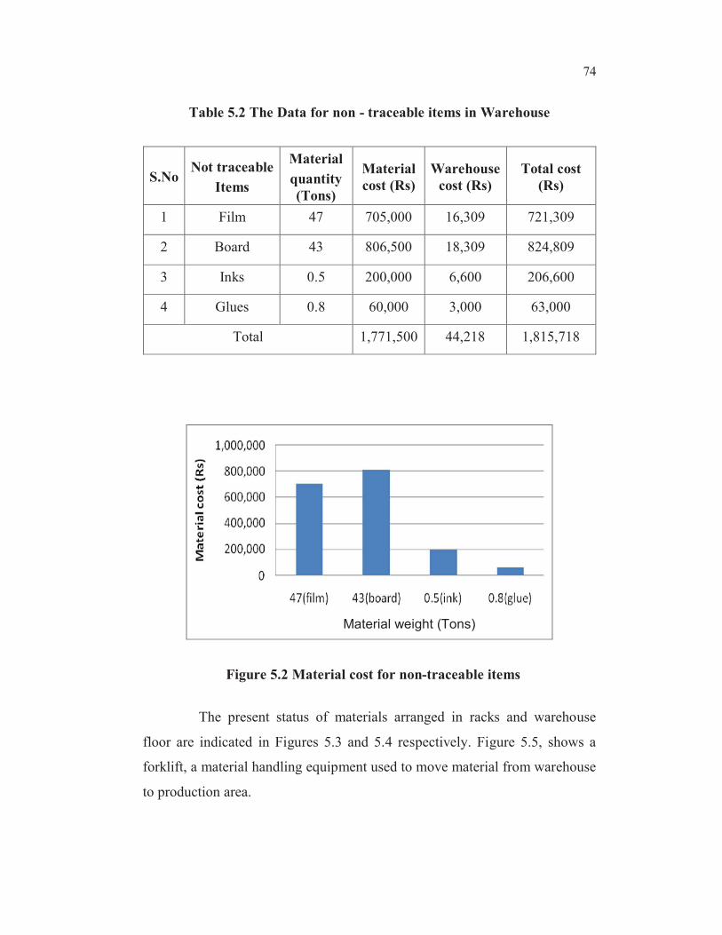
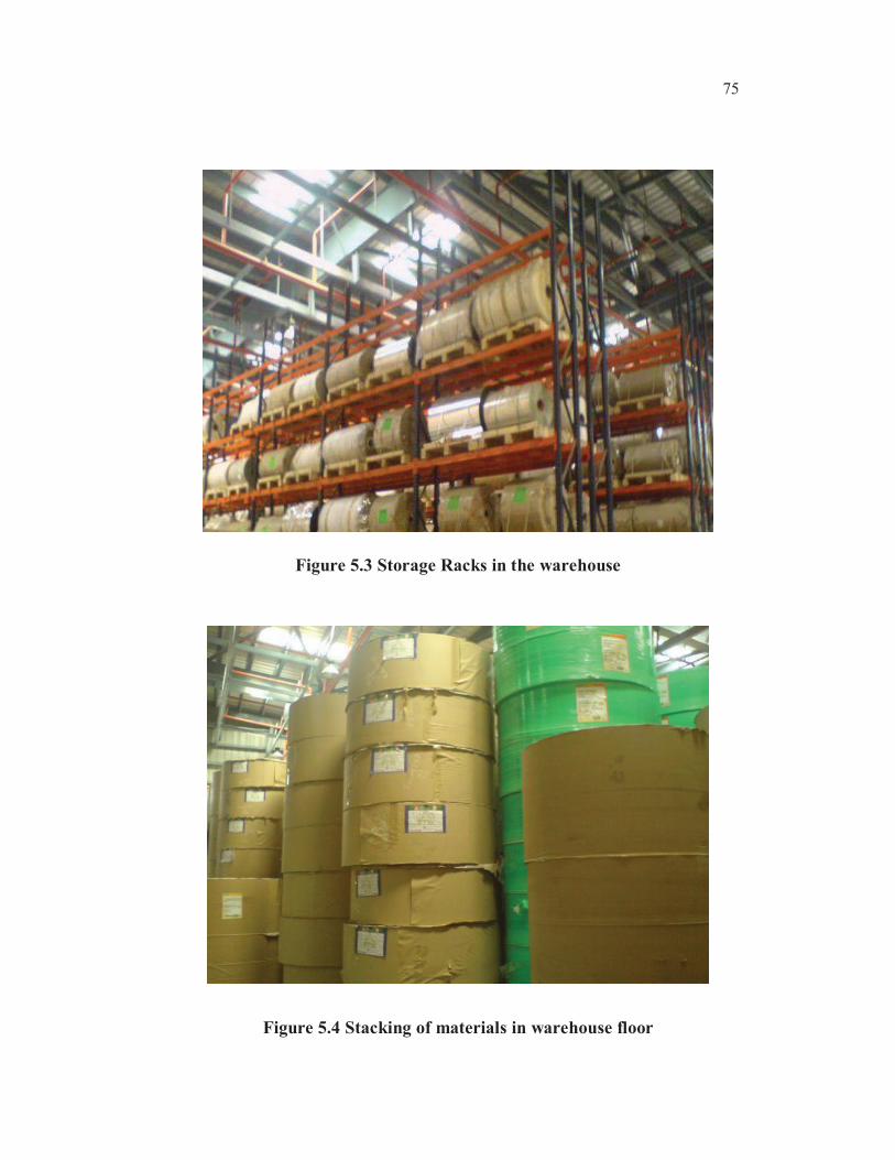
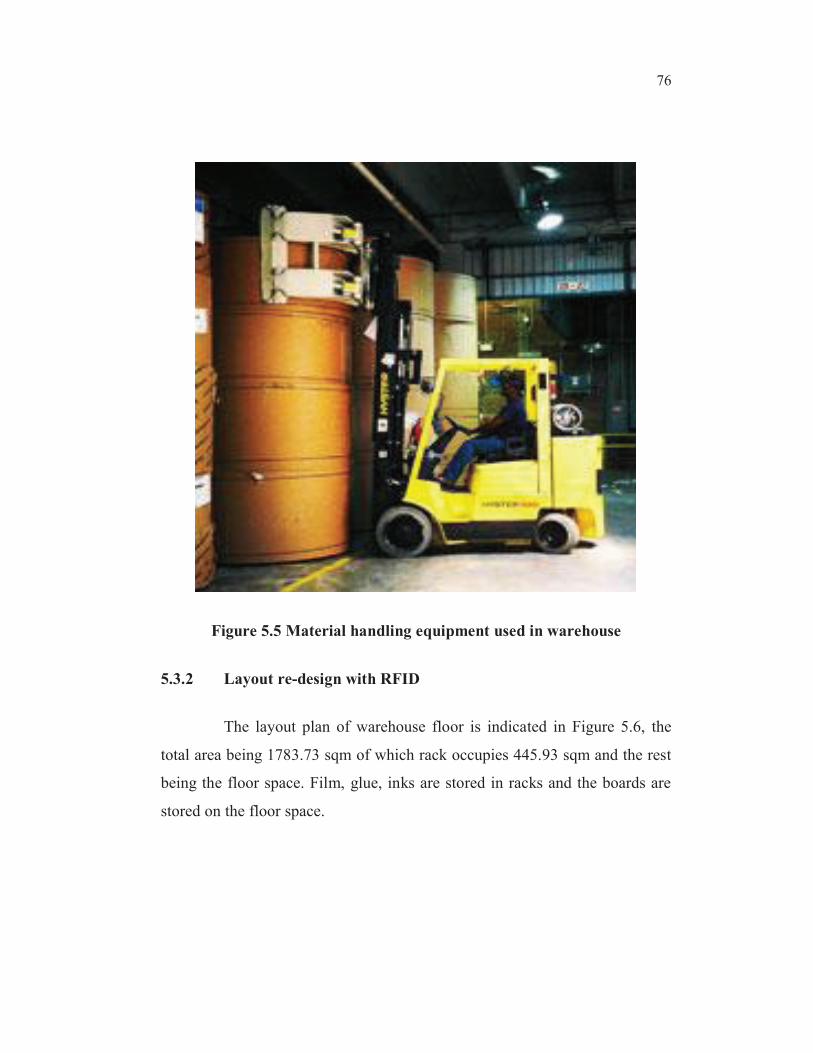
The present status of materials arranged in racks and warehouse
floor are indicated in Figures 5.3 and 5.4 respectively. Figure 5.5, shows a
forklift, a material handling equipment used to move material from warehouse
to production area.
Material weight (Tons)
75
Figure 5.3 Storage Racks in the warehouse
Figure 5.4 Stacking of materials in warehouse floor
76
Figure 5.5 Material handling equipment used in warehouse
5.3.2 Layout re-design with RFID
The layout plan of warehouse floor is indicated in Figure 5.6, the
total area being 1783.73 sqm of which rack occupies 445.93 sqm and the rest
being the floor space. Film, glue, inks are stored in racks and the boards are
stored on the floor space.

77
Figure 5.6 Layout of warehouse
Radio frequency identification (RFID) technology has been widely
used in many areas of supply chain such as manufacturing, distribution of
physical goods, inventory management etc. Although RFID is primarily an
automatic identification and data collection technique, it has made a
significant contribution to resource management in warehouse. The RFID
architecture shown in Figure 5.7 depicts the warehouse design for RFID
technology.
Storage racks
Storage racks
Storage racks
Storage racks
Paper reels
Paper reels
Paper reels
Paper reels
Floor area

78
Figure 5.7 System architecture of RFID
79
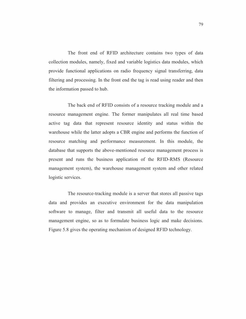
The front end of RFID architecture contains two types of data
collection modules, namely, fixed and variable logistics data modules, which
provide functional applications on radio frequency signal transferring, data
filtering and processing. In the front end the tag is read using reader and then
the information passed to hub.
The back end of RFID consists of a resource tracking module and a
resource management engine. The former manipulates all real time based
active tag data that represent resource identity and status within the
warehouse while the latter adopts a CBR engine and performs the function of
resource matching and performance measurement. In this module, the
database that supports the above-mentioned resource management process is
present and runs the business application of the RFID-RMS (Resource
management system), the warehouse management system and other related
logistic services.
The resource-tracking module is a server that stores all passive tags
data and provides an executive environment for the data manipulation
software to manage, filter and transmit all useful data to the resource
management engine, so as to formulate business logic and make decisions.
Figure 5.8 gives the operating mechanism of designed RFID technology.

80
Figure 5.8 Operating mechanism of RFID
81
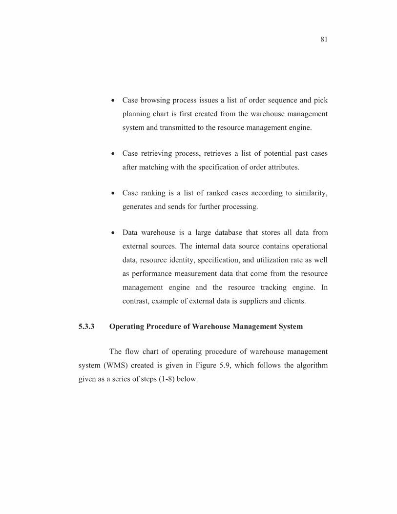
Case browsing process issues a list of order sequence and pick
planning chart is first created from the warehouse management
system and transmitted to the resource management engine.
Case retrieving process, retrieves a list of potential past cases
after matching with the specification of order attributes.
Case ranking is a list of ranked cases according to similarity,
generates and sends for further processing.
Data warehouse is a large database that stores all data from
external sources. The internal data source contains operational
data, resource identity, specification, and utilization rate as well
as performance measurement data that come from the resource
management engine and the resource tracking engine. In
contrast, example of external data is suppliers and clients.
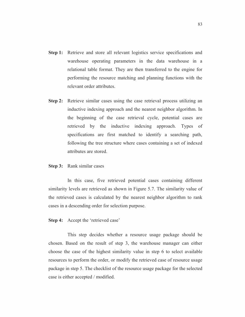
5.3.3 Operating Procedure of Warehouse Management System
The flow chart of operating procedure of warehouse management
system (WMS) created is given in Figure 5.9, which follows the algorithm
given as a series of steps (1-8) below.

82
Step 1 Retrieve relevant
pick order attribute
Step 2 Retrieve and
compare similar cases
Step 3 Rank similar
cases
Step 6 Select available
equipment
Step 4
Accept
Yes/No
Step 7 Delivery order to
loading bay
Step 8 Retain the case
Step 5
Modify
resource
package
Warehouse
management
system
Resource
management
engine
Data
warehouse
Case based
repository
Resource
tracking
module
Real time
equipment
location
Equipment
specification
Pick
order of
monitor
List of resource
package
Updated pick
order
No
Yes
Productlocation
dimensionweightFIFO
delivery
location
Figure 5.9 Operating procedures of WMS
83
Step 1: Retrieve and store all relevant logistics service specifications and
warehouse operating parameters in the data warehouse in a
relational table format. They are then transferred to the engine for
performing the resource matching and planning functions with the
relevant order attributes.
Step 2: Retrieve similar cases using the case retrieval process utilizing an
inductive indexing approach and the nearest neighbor algorithm. In
the beginning of the case retrieval cycle, potential cases are
retrieved by the inductive indexing approach. Types of
specifications are first matched to identify a searching path,
following the tree structure where cases containing a set of indexed
attributes are stored.
Step 3: Rank similar cases
In this case, five retrieved potential cases containing different
similarity levels are retrieved as shown in Figure 5.7. The similarity value of
the retrieved cases is calculated by the nearest neighbor algorithm to rank
cases in a descending order for selection purpose.
Step 4: Accept the ‘retrieved case’
This step decides whether a resource usage package should be
chosen. Based on the result of step 3, the warehouse manager can either
choose the case of the highest similarity value in step 6 to select available
resources to perform the order, or modify the retrieved case of resource usage
package in step 5. The checklist of the resource usage package for the selected
case is either accepted / modified.

84
Step 6: Select available equipment to perform the order according to the
result of selecting checklist of resource usage package in Step 4,
with the two types of preferable material handling equipment:
electrically powered pallet truck and forklift with slip sheet.
Step 7: Pick order at storage zone. Once the driver reaches the right picking
location and picks up the pallet needed for the production, the RFID
tag reader on the forklift will automatically read the RFID tag on the
pallet when the pallet comes within the reading range of the RFID
reader. The tag data is transmitted to the forklift’s computer to
verify the identity and quantity of the picked item. If the ordered
pallet contains the right product in the right quantity, the computer
of the forklift will transmit the order information to the warehouse
management system so that the inventory and storage zone status
will automatically be updated.
Step 8 : When the shipped order passes the loading bay, the reader on the
forklift will automatically read the RFID tag located at the side of
the dock door. In doing so, the real time order status will be updated
and recorded in the warehouse management system.
5.3.4 Results of Layout Redesign to Incorporate RFID in Warehouse
Management
The layout has been modified to incorporate RFID in the Warehouse
management system. An intelligent system incorporating CBR technique with
automatic data identification has been proposed. The architecture of the RFID
and the operating procedure of warehouse management system has been
designed and developed.
85
5.4 ARTIFICIAL NEURAL NETWORKS
A neural network is a software (or hardware) simulation of a
biological brain (sometimes called Artificial Neural Network or “ANN”). The
purpose of a neural network is to learn to recognize patterns in the data. Once
the neural network has been trained on samples of the data, it can make
predictions by detecting similar patterns in future data. Software that learns is
truly “Artificial Intelligence”). An inventory item having a slower rate of
consumption than the average consumption in the inventory is called slow
moving inventory item. It reduces the profit because capital is locked in the
inventory. The traditional forecasting approach in the study of inventory
systems is to give more importance to items whose demands are either large
or very difficult to forecast. Since less importance is given to inventory items
with small demand the study and analysis of slow moving inventory items
gains significance.
5.4.1 ANN model development
The brain is a collection of about 10 billion interconnected neurons.
Each neuron is a cell that uses biochemical reactions to receive process and
transmit information. A neurons dendrite tree is connected to a thousand
neighbouring neurons. When any one of the neurons is fired, a positive or
negative charge is received by one of the dendrites. The aggregate input is
then passed on to the soma (cell body). If the aggregate input is greater than
the axon hillocks threshold value, then the neuron fires, and the output signal
is transmitted down the axon. Neural networks were first introduced by
McCulloch and Pitts (1943). Neural networks are non linear mapping systems
that consist of simple processors, which are called neurons, linked by
weighted connections (Robert Schalkoff 2000).
It is vital to adopt a systematic approach in the development of
ANN models, taking into account factors such as data pre-processing, the
86
determination of adequate model inputs and a suitable network architecture,
parameter estimation (optimisation) and model validation (Maier and Dandy
1998). In addition, careful selection of a number of internal model parameters
is required. The following steps describe the methodology in developing the
artificial neural networks (ANN) model in Matlab software using “NNet
toolbox”.
The following steps describe the methodology in developing the
ANN model.
Step 1: Create network and input values of hidden neurons and desired
output
Step 2: Initialize the weights and the bias term
Step 3: Simulating the Network
Step 4: Training the Network
Step 5: Simulate using MATLAB
Step 6: Model Validation
5.4.2 ANN parameters
The simulation parameters are described below; two input nodes
indicate board sizes and seasonal months. Output node is weight of slow
moving boards and three numbers of hidden layers has used with Levenberg-
Marquardt back propagation algorithm. Twenty learning patterns are used for
training and predicting the ten patterns.
5.4.2.1 Back propagation
The term back propagation is used to imply a backward pass of error
to each internal node within the network. A back propagation consists of at
least three layers of units namely input layer and one intermediate hidden
layer and an output layer. Inputs are applied at the input layer as (pi) and
87
outputs are obtained at the last layer. A multilayer perception trained with
back propagation algorithm may be viewed as a practical way of performing a
non linear input-output of a general structure.
5.4.2.2 Training the network
Creating the network is the first step in the development of the
ANN. The function ‘newff’ creates a feed forward network. The training
function used was ‘trainlm’ given in Equation (5.1)
net = newff (p,t,3,{},'trainlm'); (5.1)
This command creates the network object and initializes the weights
and biases of the network; therefore network is ready for training. The
number of input parameter in the work was two, namely size of the board and
month. Hence they were the first input nodes and the number of output nodes
is one, namely, quantity of slow moving materials in tones. The number of
hidden nodes depends on the accuracy of the model. Here one hidden layer is
used with three neurons. The network is trained with twenty data. Training is
the learning process by which input and output data are repeatedly presented
to the network. This process is used to determine the best set of weights for
the network, which allows the ANN to classify the input vectors with a
satisfactory level of accuracy.
5.4.2.3 Simulating the network
The function ‘sim’ simulates the network. ‘sim’ takes the network
input ‘p’ and the network objects ‘net’ and returns the network output ‘a’ as
given in Equation (5.2)
a = sim (net, p) (5.2)
88
5.4.2.4 Validating the model
After the network was trained, the holdout data (consisting of 10
data) were entered into the system, and trained ANN was used to test the
selection accuracy of the network for 10 data. This is where the predictive
accuracy of the machine learning techniques is measured. The validation of
ANN model was done by testing the prediction accuracy of the model with
the actual values that were not used to train the model.
5.4.2.5 Evaluating the performance index
In order to compare the performance of each of the forecasting
methods various measures of accuracy are utilised. One measure commonly
used in inventory control is the mean absolute deviation (MAD) and mean
average percentage error (MAPE). A desirable feature of MAD and MAPE is
that it is less affected by outliers than other measures, which Wright et al
(1986) noted as being of particular importance in practical forecasting
situations where outliers are a frequent occurrence.
In order to evaluate the accuracy and performance of the network,
this work adapts Mean Absolute Percentage Error (MAPE) to evaluate the
performance in each model and is given in Equation (5.3).
MAPE=1/an
i 1
(Fi – Ai / Ai ) (5.3)
where ‘Fi’ is the expected value for the period ‘i’, ‘Ai’ is the actual value for
the period ‘i’ and ‘a’ is the number of periods. The smaller the values of
MAPE, the better the forecasting models. Having smaller values means that
the calculating results are closer to the historic data generation of slow
moving items. ANN prediction results are discussed in details in chapter 7.
89
5.5 RUNGE-KUTTA METHOD
Existing mathematical models fit well for slow moving items on
yearly basis only (James and Krupp 1977, Richard and Richard 1992). For
weekly and monthly bases a new model based on modified Runge-Kutta
method is proposed for identifying the slow moving items on weekly and
monthly bases in addition to yearly basis. The conventional Runge-Kutta
method is tedious and time consuming and hence a modification is imposed
and used for identifying the slow moving items in stock (Richard and Richard
1984).
5.5.1 Illustration of Runge-Kutta Method
The following inputs are needed for the Runge-Kutta method.
(i) Board size
(ii) Period (month of survey)
(iii) Actual board weight in Tons (stored in the variable ‘x’)
(iv) Predicted board weight in Tons (stored in the variable ‘y’)
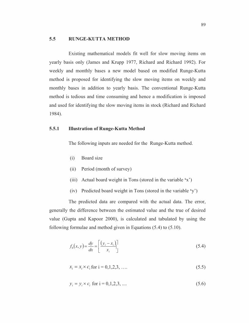
The predicted data are compared with the actual data. The error,
generally the difference between the estimated value and the true of desired
value (Gupta and Kapoor 2000), is calculated and tabulated by using the
following formulae and method given in Equations (5.4) to (5.10).
i
ii
x
xy
dx
dyyxf ,0 (5.4)
iii cxx for i = 0,1,2,3, …. (5.5)
iii cyy for i = 0,1,2,3, .... (5.6)
90
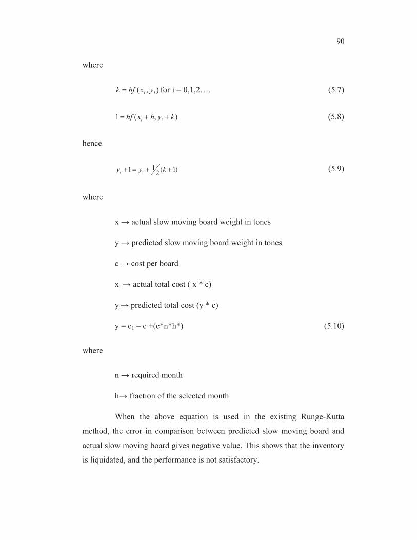
where
),( ii yxhfk for i = 0,1,2…. (5.7)
),(1 kyhxhf ii (5.8)
hence
)1(2
11 kyy ii (5.9)
where
x actual slow moving board weight in tones
y predicted slow moving board weight in tones
c cost per board
xi actual total cost ( x * c)
yi predicted total cost (y * c)
y = c1 – c +(c*n*h*) (5.10)
where
n required month
fraction of the selected month
When the above equation is used in the existing Runge-Kutta
method, the error in comparison between predicted slow moving board and
actual slow moving board gives negative value. This shows that the inventory
is liquidated, and the performance is not satisfactory.
91
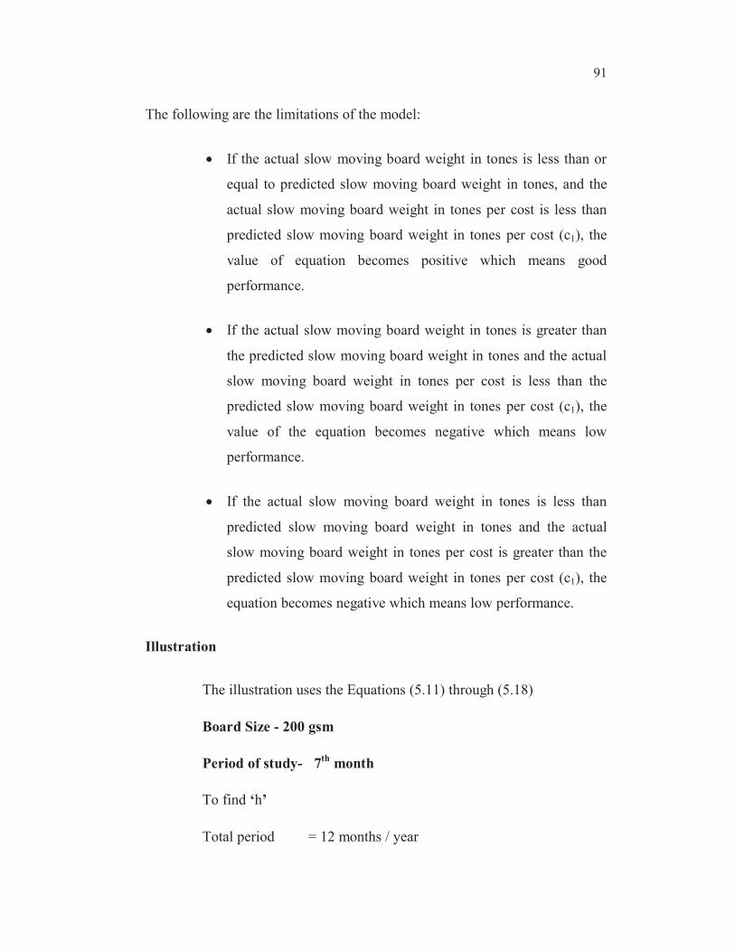
The following are the limitations of the model:
If the actual slow moving board weight in tones is less than or
equal to predicted slow moving board weight in tones, and the
actual slow moving board weight in tones per cost is less than
predicted slow moving board weight in tones per cost (c1), the
value of equation becomes positive which means good
performance.
If the actual slow moving board weight in tones is greater than
the predicted slow moving board weight in tones and the actual
slow moving board weight in tones per cost is less than the
predicted slow moving board weight in tones per cost (c1), the
value of the equation becomes negative which means low
performance.
If the actual slow moving board weight in tones is less than
predicted slow moving board weight in tones and the actual
slow moving board weight in tones per cost is greater than the
predicted slow moving board weight in tones per cost (c1), the
equation becomes negative which means low performance.
Illustration
The illustration uses the Equations (5.11) through (5.18)
Board Size - 200 gsm
Period of study- 7th
month
To find ‘h’
Total period = 12 months / year

92
One month = 1h = 1/12 of a year
h = 1/12
h = 0.083
For 7th
month = 7h = 7 x 0.083 = 0.581
In the existing Pareto Analysis the slope of the equation is given by
the function f (x,y)
f(x,y) = [dy/ dx] = [ (y-x) / x ] (5.11)
Where y = Predicted slow moving board weight in tones
and x = Actual slow moving board weight in tones
y(xo) = yo (5.12)
xo = 0.58, yo= 0.018,
Also y1 = yo +1/2 (k+l) (5.13)
Where k = h f (xo, yo) = h [ (yo - xo)/ xo ] (5.14)
k = 0.083 [(0.018-0.58) / 0.58]
k = - 0.080
Also l = h f (xo+h yo+k) (5.15)
l = 0.083 f (0.58 +0.083,0.018 + (-0.080) )
l = 0.083 f (0.663, -0.062)
= 0.083 [(yo - xo)/ xo]
l = 0.083 [(-0.062 -0.663) / 0.663]
l = -0.090

93
Substituting in (5.13)
y1 = yo +1/2 (k+l)
= 0.018 +1/2 (-0.080-0.90)
y1 = -0.067
y(xo) = yo
y(0.663) = -0.067
(y1 for 7th
month becomes the value of yo for the 8th
month)
Board size = 200gsm
Period of study = 8th
month
y(xo+h) = yo (5.16)
y(0.58+0.083) = -0.067
y (0.663) = -0.067
now xo = 0.663 and yo = -0.067
and k = 0.083 f(0.663, -0.067)
k = 0.083 [(-0.067-0.663) / 0.663]
0.730k 0.083 0.091
0.663
also l = 0.083 f(0.743, - 0.0158)
1006.0743.0
743.00158.0083.01

94
Substituting in (5.16)
y1 = -0.1628
i.e y(xo) = yo
y(0.743) = -0.1628
(y1 for the 8th month becomes the value of y0 for the 9
th month)
Now
y(0.663) = -0.067
y(0.743) = -0.1628
Hence it is proved that in the conventional Runge-Kutta method, for
board size of 200 gsm, the slow moving inventory items yield negative
equations, in all those months which is considered as low performance level.
Now it is possible to generalize the Runge-Kutta method using the
following formulae given in Equations (5.17) through (5.20), which can be
used for finding the slow moving inventory behaviour of other board sizes of
215 gsm, 240 gsm, 300 gsm, and 400 gsm.
i
iii
x
xyy for all i = 0,1,2,3,….. (5.17)
where k= h f (xi ,yi) for all i = 0,1,2,3,….. (5.18)
l = h f (xi +h, yi + k) for all i = 0,1,2,3,….. (5.19)
and
yi +1 = yi +1/2 (k+l) for all i = 0,1,2,3,….. (5.20)
95
5.6 SUMMARY
The existing models are very less efficient while dealing with real
life industrial data sets, whereas this proposed model is tested and proved
efficient with real life industrial data sets. It requires only the functional
values at some selected points on the sub intervals which are a major
advantage of this model. Further this model is flexible and capable to analyze
large number of items. It employs the simple screening rule to identify the
slow moving inventory items. The analysis of this system is simple and more
realistic. Since this system is associated with cost parameter, keeping of
inventory item for long period may not be treated as having the effect of slow
moving item. In this model ordering policy and distribution are associated
with cost and hence less frequency of ordering period of item may not be
considered as slow moving item. The main limitation of this model is its
dependence on historical data.