5 - 1

Chapter 5. RF Systems

M. Champion, W. Chou, J. Griffin, K. Koba, J. MacLachlan, A. Moretti,M. Popovic, Z. Qian, J. Reid, J. Steimel, D. Wildman

5.1. Introduction

In this section two completely separate Proton Driver rf systems are described. Becauseof space limitations in the lattice it will not be possible to install and/or operate the twosystems concurrently. For Stage 1 operation, a 37 - 53 MHz rf system will be installed.Development for this application of a large aperture (5"), increased voltage modificationof an existing Fermilab Booster rf cavity is described in Sec. 5.2.2. As an alternative,efforts have begun on modification of the TRIUMF/SSC style orthogonally biased ferriterf cavity, cf. Sec. 5.2.3.

For Stage 2 operation the 53 MHz system will be removed, and a lower frequency,harmonic number 18, rf system will be installed. For this system, development of an rfcavity using a new nanocrystalline soft magnetic material, Finemet, is described in Sec.5.3.2. The lower frequency cavities may use some ferrite tuner components obtainedfrom the removed 53 MHz cavities for tuning during acceleration.

The rf parameters for the two stages are summarized in Table 5.1.

Table 5.1. Summary of RF Parameters

Stage 1 rf parameters (Section 5.2) Stage 2 rf parameters (Section 5.3)Harmonic number 126, with 119 occupied

buckets.Extraction longitudinal emittance, (95%),

0.1 eV-s per bunch.Rf frequency range: 37.8 - 53 MHz.Maximum ring voltage: 1.2 MV.Average rf power to beam (66.6 ms period)

~ 835 kWPeak rf power to beam capability ~2 MW.

Harmonic number 18, with all bucketsoccupied.

Extraction longitudinal emittance, (95%),0.4 -0.5 eV-s per bunch.

Rf frequency range: 5.4 - 7.6 MHz.Maximum ring voltage: 1.4 MVAverage rf power to beam (66.6 ms period)

~1.2 MW.Peak rf power to beam capability ~ 2.9

MW.Extracted bunch length ~ 1 ns rms

(neutrino source operation).

Section 5.2, (Stage 1), describes an rf system which is consistent with use of theProton Driver as an injector for the Main Injector ring in "normal" operation. In thismode the ring will operate from injection energy 400 MeV to extraction energy 12 GeVwith intensity ~3 × 1013 protons per cycle. The guide fields will be sinusoidal at 15 Hz,with a 12.5% second harmonic component, phased so as to optimize certain rf voltageand bucket area parameters.

5 - 2

Section, 5.3, (Stage 2), describes an rf system to be used in neutrino source service,but also capable of injecting widely spaced intense bunches into matched Main Injectorbuckets. In this mode the extraction energy will be 16 GeV with beam intensity 3 × 1013

protons per cycle. Guide field parameters will be similar to those described above.

In each case the rf accelerating voltage, Vsinϕs, is defined uniquely by the ringcircumference and the rate of rise of the magnetic guide field, dB/dt. The additional rfvoltage necessary to obtain the design intensities, longitudinal emittances, and bunchconfigurations proposed for each of the Proton Driver stages have been elucidatedthrough extensive simulations of rf capture, acceleration, and bunch manipulation prior toextraction, using the code ESME. In each case the effect of installation of space chargecompensating inductance (see Section 5.1.1) has been included in the calculations. Also,the higher harmonic effects of frequency variation of the parameters of the introducedinductance have been simulated. Descriptions of these simulations and their results forStage 1 and Stage 2 acceleration are presented in 5.2.1, 5.2.2, 5.3.1, and 5.3.2. Forinjection into the Main Injector, the rf voltage and bucket area will be adjusted duringacceleration such that extracted bunches will be matched to stationary buckets in theMain Injector. In neutrino source application, the rf voltage will be manipulated prior toextraction so that the extracted bunch length will be ≤ 1 ns rms.

5.1.1 Beam Loading.

With intensity 3 × 1013 protons per cycle, design techniques for compensation of variousforms of beam loading must be incorporated. This is especially true in Stage 2, where, ath = 18, the charge per bunch will be 1.67 × 1012 protons per bunch (0.27 µC). Theamplitude and phase of the net rf voltage will be affected by cavity excitation byfundamental and lower harmonic Fourier components of the beam current. These beamloading errors are to be corrected by a global feedback system in which unwanted beamphase motion, detected by broad-band beam pick-ups, will be compensated for bycorrection signals delivered to each rf station. Global feedback systems are described in5.2.4, 5.2.6, 5.3.3, and 5.3.5.

Below transition the charges in each bunch interact with the vacuum chamberconducting wall in such a way as to reduce the rf focusing force and bucket area [1]. Ithas been pointed out, by A. Sessler and V. Vaccaro [2], that this "potential welldistortion" may be minimized by the intentional introduction of inductance into thevacuum chamber.

The effect of installed inductance has been studied in the KEK Proton Synchrotron.Because the potential well distortion moves with the charge distribution, the coherentsynchrotron dipole phase oscillation frequency is not affected. Predicted changes inincoherent phase oscillation frequency, representing changes in the bucket area, wereobserved by measurement of the synchrotron quadrupole frequency as a function of beamintensity with fixed rf voltage [3,4].

5 - 3

In a Fermilab-Los Alamos collaboration experiment, inductances sufficient to cancela large fraction of the space-charge potential well distortion were installed in the LosAlamos Proton Storage Ring (PSR). The PSR beam intensity has been limited by theonset of a transverse ep instability caused by electrons trapped in the proton beampotential well. An h = 1 rf bunching system is operated to create a gap in the proton beamto allow trapped electrons to escape. With increasing beam intensity the effectiveness ofthe rf system is compromised by beam induced potential well distortion, and smallnumbers of protons escape the rf generated potential well and drift into the gap. Initialresults of the experiment indicated that the inductors increased the effectiveness of the rfbunching system such that significantly larger beam intensities could be attained [5,6].

Because of the geometry of the introduced ferrite rings and the real and imaginaryproperties of the ferrite permeability at high frequency, the installed inductors caused anunacceptable self-bunching (microwave-like) instability. This problem was solved byheating the ferrite in such a way that the Q and the shunt impedance of the offendingresonance were reduced so that no instability occurs at the PSR design intensity. Anadded benefit of the heating is that the real permeability of the ferrite is increased to alevel such that the installed inductors almost exactly cancel the beam-induced distortion.No additional inductance was required to reach the design intensity.

The Proton Driver design group will take advantage of the added inductance tominimize the requirement for installed rf capability in the 53 MHz Stage 1 design. It mayalso be useful to utilize installed inductance to enhance the performance in Stage 2following injection capture and during bunch manipulation to create narrow bunches.

5.1.2 Direct Space Charge Compensation

As the 0.27 µC charges in each bunch (Stage 2) pass through the gap capacitance C ofeach rf cavity, a decelerating voltage approaching q/C may be developed, so that thecharges in the bunch do not all see the same accelerating voltage. If, for instance, theeffective gap capacitance were 100 pF, the voltage developed may reach 2.7 kV, asignificant fraction of the design gap voltage. The developed voltage may be reduced byincreasing the effective gap capacitance (effectively lowering the cavity Rs/Q). Atsignificantly higher beam intensity (a future possibility), the effect may be counteredthrough the addition of a second power amplifier tube with its anode connected directlyto the down-stream side of the gap capacitance. This additional tube may be pulsed in afeed-forward configuration so that it delivers an electron charge to the gap capacitorapproximately equal to the beam bunch charge during the bunch passage, thusminimizing the pass through charging effect of the beam.

5.1.3 Single Frequency High Gradient Burst Mode RF Cavity

Research and development for a very high gradient fixed low frequency rf cavity,(~ 600 kV per meter), is in progress here and at KEK Japan. Such a cavity could beinstalled to add to the rf voltage during bunch rotation for the development of narrowbunches at extraction.

5 - 4

5.2. Stage 1 (53 MHz) RF

5.2.1 RF Voltage, ϕϕϕϕs, Bucket Area, Simulations

In Phase I the Proton Driver is used with the Main Injector and possibly a neutrinofactory; the defining property is a beam intensity of 3.0 × 1013 protons/pulse. In Stage 1the Proton Driver serves only to replace the present Booster for injection into the MainInjector and possibly for low energy neutrino production. It will employ refurbishedBooster rf cavities, modified to give a 5 inch aperture. The design parameters used todefine the rf requirements for Phase I, Stage 1 are collected in Table 5.2.

Table 5.2. Stage 1 Proton Driver rf Parameters

Einj injection kinetic energy 400 MeVBeam intensity 3 × 1013 p/cycleCycle repetition 15 Hz

Eex extraction kinetic energy 12 GeVReq circumference/2π 113.21 mVrf maximum rf voltage 1.2 MVVacc accelerating voltage at dp/dt max 1.09 MVh harmonic number 126

number of populated buckets (at extraction) 119εl longitudinal emittance at extraction 0.1 eV-s

bunch intensity 2.5 × 1011

∆Einj energy spread at injection ±0.5 MeVα0 momentum compaction -1.306 × 10-3

α1 coefficient of (∆p)2 in path length 8.252 × 10-2

b vacuum chamber radius 6.35 cma mean beam radius at injection 4.44 cm

The combination of performance demands with the mandated use of the 400 MeVLinac injector and modified Booster cavities calls for some unconventional measures.The specified intensity and emittance put the Proton Driver into the class of highbrightness synchrotrons. The space charge impedance corresponding to the perfectlyconducting wall force is Z||/n ≈ -340i Ω at injection energy. To control the space chargedefocusing, a tunable inductive insert is proposed, which will cancel this impedancethroughout most of the cycle. The insert looks very attractive in the modeling; it makesthe difference between 96.8 % and 99.99% for the particle transmission efficiency of thecomplete cycle. The idea is not new [2]; it has been tried in two different machines(Section 5.1.1). However, the studies have not been carried out over a wide range ofbeam energy or momentum spread and more beam studies are needed.

The next subsection gives curves for the time dependence of parameters, whichchange during the acceleration cycle; it is followed by a subsection with details of the

5 - 5

scenario, beam physics, and description of the optimization process, considerationssubstantially reducing the scope for arbitrary choice of the parameter curves.

5.2.1.1. Parameter Programs – Stage 1 RF Curves

The magnet ramp is driven by a 15 Hz resonant power supply plus an independent secondharmonic supply that is adjusted in phase and amplitude to minimize the required peak rfvoltage. The fixed parameters are those in Table 5.2. The design optimization has beencarried out primarily by multi-particle tracking simulation; the results include the timecurves, a demonstration of potential for low loss operation, and a demonstration that thespecification for longitudinal emittance at extraction is reasonable. Because the rf voltagelimit is so stringent, loss limitation naturally relates closely to longitudinal emittancepreservation.

The curves in Figs. 5.1 - 5.5 present the momentum p, its time derivative dp/dt, thepeak rf voltage Vrf, the synchronous phase φs, and the h = 1 reactance of the inductiveinsert. In this last case, three optimum levels with optimum break times are shown. Alsoshown is a continuous dotted curve, calculated to just cancel the space charge force. Theissues related to the optimum for this curve are examined in the following subsection.

Figure 5.1. Beam Momentum, MeV/c

Figure 5.2. Rate of change of momentum, dp/dt vs. time, Stage 1

5 - 6

Figure 5.3. Stage 1 rf voltage in MV

Figure 5.4. Synchronous phase angle, φs, during Stage 1 acceleration

Figure 5.5. Reactance of the inserted inductor at rotation frequency (h = 1) as a functionof time during acceleration

5 - 7

The curves in Figs. 5.6 - 5.8 present useful derived quantities, viz., synchrotron tuneνs, bucket area SB, and the rms longitudinal emittance per bunch εl.

Figure 5.6. Small amplitude synchrotron tune, units of Frot

Figure 5.7. Stage 1 rf bucket area, eV-s

Figure 5.8. Stage 1, rms longitudinal emittance, eV-s

5 - 8

5.2.1.2. Capture and Acceleration – Stage 1 Scenario and Modeling

A macro-particle tracking model has been used for the entire cycle from multi-turninjection through matching to Main Injector buckets. The injected protons are assumed tobe a continuous coasting beam lasting up to 90 µs, timed symmetrically about dB/dt=0.Other timings have been tried as well, but for an injection period this short nothing betterhas been found. For nominal Linac intensity, 70 µs is sufficient to give the required3 × 1013 protons, but efficiency remains good over a longer injection time. A goodapproximation is to represent continuous injection by injections every other turn. Thebeam charge is raised in concert with the macro-particle injection; the perfectlyconducting wall term and the inductive insert are the only sources of the collectivepotential included in these simulations.

The rf voltage is raised linearly during injection from 0 to 65 kV. Because of the largeslip factor η for this machine, the particles near ±180o of rf phase are all captured in thissimple maneuver. Certainly some are quite close to the separatrix and subject to later lossbecause of space charge and limited rf voltage, but these losses are essentially eliminatedby use of the inductive insert. They could also be largely eliminated with a substantiallyhigher rf voltage capability. After 226 µs, the voltage curve is changed to provide abucket area that grows slowly to 0.064 eV-s at 4.96 ms. At this time the voltage hasreached the design limit of 1.2 MV and it is held at that value until η has droppedsufficiently, at about 30 ms, to allow a reduction while continuing to increase the bucketarea. dB/dt reaches zero at 37.93 ms. The voltage required for acceleration at maximumdp/dt is 1.09 MV, so there is little rf focusing. The synchronous phase reaches 64o.Although dp/dt continues to increase, the magnet ramp has been tailored so that thebucket area does not decrease; in fact it rises slightly in the middle of the flat part of thevoltage curve. Nonetheless, in the absence of the inductive insert there are losses atmaximum dp/dt (about 0.025 s into the cycle). This indicates that the specified maximumrf voltage is marginal and the inductive insert could be very important.

There are three ways in which these modeling efforts have fed back to changesomewhat the initial design ideas. One way is that the optimum magnet ramp has beendetermined as a minimum Vrf ramp rather than a minimum dB/dt ramp. Another changeis the discovery of the apparent effectiveness of an inductive insert and its importance forlow beam loss with h = 126 rf. Finally, it was noticed that the slip factor is so high atinjection that the captured beam displays significant energy-phase correlation (bunch tilt).Precious bucket area is wasted; beam is lost because the momentum spread is increasedby the tilt. Dividing the rf into 2 parts on opposite sides of the ring made a substantialimprovement in the tilt and resulting loss. Dividing the rf into 3 equally spaced groupswould make a small additional improvement. The planned configuration of the injection,extraction, and collimation systems may be inconsistent with the 3-way division.

Table 5.3 shows the injection-to-extraction transmission efficiency and emittance atextraction for different departures from the optimum modeling result. The top entry is thebest result obtained, and each entry following gives the transmission when one conditionis changed without attempting to re-optimize the other parameters. Possibly some of the

5 - 9

apparently lost efficiency could be recovered in such a re-optimization, but the intentionis only to suggest the importance of various conditions to the optimum obtained. Thelower final emittance for the more closely grouped cavities reflects directly the removalof halo by having the bunch tilted in the early part of cycle. The 95% emittance atextraction is 0.08 eV-s for the optimum case.

Table 5.3. RMS emittance at extraction and fractional beam loss during a complete cyclefor optimum parameters and cases each differing from the optimum in a single property

Optimum case 0.0201 eV-s 0.01%All rf clumped 0.0154 eV-s 0.21%rf in two sets 0.0181 eV-s 0.07%no inductive insert 0.0247 eV-s 3.19%

Clearly the inductive insert is a significant element in this scenario; a limited amountof rf focusing is supplemented with a self-excited focusing voltage. The character of theinductance curve suggests that there is room for refinement here. It is natural to considertuning the inductance to just cancel the space charge impedance at all times, and indeedthis could be a satisfactory mode. However, it is not a straightforward matter because apure inductance will not cause instability even if it over-compensates, and extra focusingshould be helpful. There are at least three sources of real impedance which coulddecelerate self-excited bunches out of the 53 MHz bunch at some higher frequency, i.e.the inductor could cause self-trapping instability. The impedances which should be takeninto account at a minimum in constructing a good model are the resistive wall, thebroadband beam pipe impedance from miscellaneous sources (the usual Z|| /n), and theresistive component of inductor impedance. Permeability and loss factor curves for aTranstek Yttrium garnet ferrite have been used. The real impedance of the inductor isapproximated by a 45 MHz Q = 50 resonance with Rshunt = 13 kΩ; Z|| /n = 5 Ω is includedin the impedance tables that represent the inductance of the insert.

The resistive wall term is expected to be important only for the multi-bunch effects.The stability issues have not been adequately treated in the modeling, which is aimed atthe problems of bucket distortion and bucket area loss. The charge distribution issmoothed to take out high frequency fluctuations, which are principally numerical noise.Once a realistic longitudinal impedance has been specified, it will be appropriate to tracka portion of the cycle with enough macro-particles to represent the beam current Fourierspectrum up to 1 GHz or so.

The inductive insert is an important area for development in modeling and in machinestudies as well. The Fermilab Booster is a suitable machine for investigating theeffectiveness of an inductive insert, and it has also a reasonable prospect for obtaining anoperational benefit.

5 - 10

5.2.2 Fermilab Booster Cavity Upgrade

A proposal [7,8] to modify the existing Booster rf cavity was made in January, 2000. Inthis proposal, two goals were set forth: (1) to enlarge the cavity beam pipe aperture from2.25 to 5 inches; (2) to increase the cavity voltage by 20%, from 55 kV to 66 kV. Themotivation for this effort is twofold. For the existing Booster, aperture enlargement willresult in less activation of the rf cavities and power amplifiers, thereby permitting accessto the cavities for regular maintenance during future high duty factor operation.Increased cavity voltage will allow for operation with fewer than 100% of installedcavities, thereby reducing downtime due to unscheduled maintenance. For the ProtonDriver, aperture enlargement is necessary to accommodate the higher beam intensity withacceptable beam loss. The increased cavity voltage is required to increase the beamenergy from 8 to 12 GeV without increasing the acceleration cycle time.

5.2.2.1. Overview of existing Booster rf cavities.

The Booster depends on 18 rf cavities for acceleration, each cavity providingapproximately 55 kV over a frequency of 37 to 53 MHz. Hence, a ring voltage of 990 kVis achieved. (A voltage increase of 20% would raise the ring voltage to 1188 kV.) The rfcavity is a center-fed coaxial double-gap structure with an electrical length of136 degrees, gap-to-gap, as illustrated in Figure 5.9. The 150 kW power amplifier ismounted directly to the cavity and is coupled to the center conductor via a 1200 pF anodedc blocking capacitor. The cavity frequency is controlled by three ferrite-loaded variableinductors attached at the center of the cavity in parallel. The ferrite bias windings areseries connected and driven by a 2500 A programmable bias supply. Near theaccelerating gaps at each end of the cavity are 12 inch o.d. conical coaxial aluminawindows separating the beam vacuum from the air-filled center section of the cavity.The gap spacing is 0.9 inches and the beam aperture is 2.25 inches. The cavity anode togap voltage step-up ratio varies from 1.2 to 1.6 over the tunable frequency range.Figure 5.10 is a photograph of the cavity.

Figure 5.9. Detail of Booster cavity gap geometry

5 - 11

Figure 5.10. Booster cavity withferrite tuner in foreground

5.2.2.2. Prototype large apertureBooster rf cavity; apertureenlargement and tuning.

A damaged Booster rf cavity has beenthe basis of the prototype work to date.Both ceramic windows, one of whichwas already broken, were removed toallow for extraction of the cavitycenter conductor. The centerconductor was cut off along the taperon both sides of the center hub andnew 5.5 inch outside diameter endswere attached along with variablespacing gap electrodes. The 5.5 inchdiameter was chosen to allow for aninside diameter of 5 inches includingthe required vacuum beam tube and ahigh permeability cylinder intended toshield the beam from tuner magneticfields. The end plates of the cavity

were modified to match the 5 inch aperture. Gap spacing up to 3 inches can be achievedwith the prototype cavity. Alumina washers were purchased to approximate thecapacitive loading that will be present in a new vacuum window design.

As a first step, two standard Booster cavity ferrite tuners were mounted on themodified cavity prototype and measurements were performed with a special cut-awaypower amplifier that allows access to the amplifier tube anode via the screen basket. Theimpedance at the anode of the tube can be measured by inserting the probe of a vectorvoltmeter into the screen basket between the anode and screen. The ferrite tuner biascurrent is set and the frequency of the vector voltmeter is adjusted until a phase angle ofzero, (real load), is indicated. Following this procedure, curves of anode impedanceversus resonant frequency may be measured for various configurations.

Three tuner configurations were explored: two Booster tuners, three Booster tuners,and two Booster tuners with one Main Injector tuner. The resulting anode impedanceversus cavity frequency is shown in Figure 5.11. For comparison, the data for a standardBooster cavity is included. Clearly the lower inductance of the Main Injector tuner isnecessary to make up for the increased capacitance resulting from the cavity apertureincrease. Two different gap spacings were investigated: 0.9 inch and 2 inch. Asexpected, the larger gap spacing results in a slightly higher upper frequency limit due to

5 - 12

the decrease in gap capacitance. These data do not extend to higher frequencies becausethe first measurements were performed using only a 1000 A bias supply.

Booster Cavity Anode Impedance vs. Frequency

0

2

4

6

8

10

20 25 30 35 40 45 50

MHz

kž

Standard booster cavity2 BR tuners, 0.9" gap3 BR tuners, .9" gap3 BR tuners, 2" gap2 BR & 1 MI tuners, 2" gap2 BR & 1 MI tuners, 0.9" gap

Figure 5.11. Curves of prototype cavity anode impedance versus resonant frequency forvarious tuner and gap configurations

Based on the foregoing results, the prototype cavity, configured with two Boostertuners and one Main Injector tuner, was moved to the MI–60 test station, where first testswith a 2500 A bias supply were recently performed. Bias currents from 0 to 2500 Aprovided a frequency tuning range from 29.8 to 53.4 MHz with a gap spacing of 0.9inches. For comparison, a standard Booster cavity has a maximum frequency of53.3 MHz. These data are shown in Figure 5.12.

Booster Cavity Anode Impedance vs. Frequency

0

2

4

6

8

10

12

25 30 35 40 45 50 55

MHz

kž 5" prototypeStandard Booster Cavity

Figure 5.12. Curves of anode impedance versus resonant frequency comparingthe prototype and standard Booster cavities

5 - 13

5.2.2.3 Cavity shunt impedance, Q, and Rs/Q

The impedance shown is the impedance presented to the power amplifier by the cavitywith no beam loading. These impedances, coupled with the tube anode rf swing, can beused to calculate the dissipation in the cavity. However, they do not represent the trueshunt impedance of the cavity as seen by the beam. The beam effective shunt impedanceis obtained by multiplying the measured anode impedance by 4 × S2sin2∆, where S is thevoltage step-up from hub to gap and ∆ is the hub to gap electrical length.

The prototype Rs varies from ~ 11 kΩ to 56 kΩ between 30 and 50 MHz. The Q ofthe prototype cavity has recently been measured to vary from ~230 to 900 over the samefrequency range. From these data it can be inferred that the effective R/Q ranges from~50 to ~60, reaching a maximum value ~69 at 45 MHz.

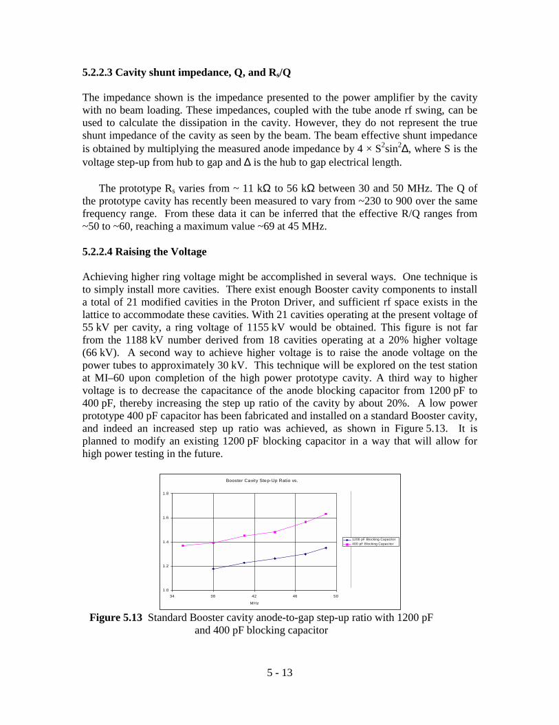
5.2.2.4 Raising the Voltage

Achieving higher ring voltage might be accomplished in several ways. One technique isto simply install more cavities. There exist enough Booster cavity components to installa total of 21 modified cavities in the Proton Driver, and sufficient rf space exists in thelattice to accommodate these cavities. With 21 cavities operating at the present voltage of55 kV per cavity, a ring voltage of 1155 kV would be obtained. This figure is not farfrom the 1188 kV number derived from 18 cavities operating at a 20% higher voltage(66 kV). A second way to achieve higher voltage is to raise the anode voltage on thepower tubes to approximately 30 kV. This technique will be explored on the test stationat MI–60 upon completion of the high power prototype cavity. A third way to highervoltage is to decrease the capacitance of the anode blocking capacitor from 1200 pF to400 pF, thereby increasing the step up ratio of the cavity by about 20%. A low powerprototype 400 pF capacitor has been fabricated and installed on a standard Booster cavity,and indeed an increased step up ratio was achieved, as shown in Figure 5.13. It isplanned to modify an existing 1200 pF blocking capacitor in a way that will allow forhigh power testing in the future.

Booster Cavity Step-Up Ratio vs.F

1.0

1.2

1.4

1.6

1.8

34 38 42 46 50

MHz

1200 pF Blocking Capacitor400 pF Blocking Capacitor

Figure 5.13 Standard Booster cavity anode-to-gap step-up ratio with 1200 pFand 400 pF blocking capacitor

5 - 14

One potential problem with increasing the voltage per cavity is the voltagebreakdown limit of the existing ferrite tuners. The stem connection is the first place tobreak down when operating at high voltages. High power rf tests with the prototypecavity will confirm the maximum operating voltage as determined by this tunerlimitation. This limitation might be overcome by increasing the length of the tuner stem,thereby inserting a series inductance over which some rf voltage will be dropped. Thiswould require a somewhat different tuning inductance with which to achieve the desiredfrequency range of 37 to 53 MHz.

5.2.3 TRIUMF RF Cavities

An alternative to rebuilding the present Fermilab Booster rf cavities is to construct twelvenew orthogonally biased rf cavities similar to the Los Alamos/SSC/TRIUMF design [9].This type of cavity offers three clear advantages. First, higher peak accelerating voltageof 100 kV/cavity (the TRIUMF cavity has been run for several two hour intervals at 50Hz at 62.5 kV on the gap) will require only two thirds the number of cavities in the ring.Secondly, the accelerating gradient of 94 kV/m is three times the 29 kV/m anticipated inthe modified Booster cavity. This reduces the total length of the rf straight sections by afactor of three. Thirdly, the use of orthogonally biased garnets instead of the present Ni-Zn ferrites reduces the rf losses in this cavity design by at least a factor of two.

The TRIUMF prototype cavity,shown in Figure 15.14 is now atFermilab. It has a 6 inch aperture and istunable from 36 to 53.4 MHz. Tuning isprovided by six, 60 cm OD × 30 cm ID,Trans-Tech G810 aluminum dopedyttrium garnet rings. These rings areorthogonally biased by a toroidal C-magnet excited by bias current from 500to 1050 amps. The TRIUMF cavity Qranges from 240 to 2000 and the shuntimpedance increases from 12.4 kΩ to88 kΩ as the resonant frequency israised. The cavity final amplifier ispowered by an Eimac Y567B tetrode,identical to those used in the presentBooster, Main Injector, and Tevatron rfsystems.

Figure 5.14. TRIUMF PrototypeCavity

An additional six months ofdevelopment work would be useful in

evaluating the TRIUMF cavity. One item that needs further investigation is the cavity’s

5 - 15

non-linear frequency response at high rf magnetic fluxes. This effect, also observed insome ferrites, is characterized by a shift in the cavity’s resonant frequency to a lowerfrequency as the gap voltage approaches its maximum value. This frequency shifting willadd an extra complication to dynamically tuning the cavity during acceleration.However, it is anticipated that a fast feedback loop around each rf station should be ableto keep the cavity tuned to the correct frequency.

5.2.4 Steady State Beam Loading, Robinson Detuning.

Robinson’s inequalities for maintaining longitudinal stability in the presence of beamloading are shown below. The first inequality states that the cavities must be tuned suchthat the fundamental frequency lies just below the resonant frequency of the cavity(below transition). The ferrite tuning loops automatically maintain this condition.

The second inequality states that the cavities must deliver more power to the beamthan the beam delivers to the cavity. Assuming that each cavity can deliver about 30kVto a gap with a shunt impedance of about 15 kΩ, the ratio of the beam current withrespect to the in phase current of the cavity is about 1. This is still considered stable, butit is very close to becoming unstable.

The transient voltage caused by the six-bucket extraction kicker gap in the beam isless than 0.1% of the total accelerating voltage. Since transient compensation will not benecessary, only fundamental compensation is required. The same system used in theMain Injector for fundamental feedback can be modified for use in the Booster. It canprovide an increase in the beam current threshold by about a factor of 14 (assuming aboutthe same group delay from cavity drive to the gap). This will allow the RF voltage to bedecreased to about 85 kV before beam loading becomes significant.

5.2.5 Stage 1 (37 - 53 MHz) RF Cavities, Power Supplies, Total Power, Water

Table 5.4 summarizes equipment and installation requirements.

Table 5.4. Equipment and installation requirements

37 - 53 MHz RF Cavities 20 Existing Booster Cavities Modified for 5 inch ApertureHigh Level RF 20 High Level Booster Stations Required.

Use 18 existing Ferrite Bias SuppliesUse 18 existing IRM station control & data acquisition systems

New Equipment; (20) - 200 kW Power Amplifiers.(20) - 30 kV Series Tube Modulators(20) - 6 kW Solid State Wide band Drivers.(2) - Additional Ferrite Bias Supplies (0-2500A).(2) – 35 kV Anode Power Supplies.

0 sin 2 Ψ z< 2 Ycos Ψ B< YI B

Re I T

5 - 16

Existing Booster cavities will be modified to increase their aperture from 2-1/4 inch to 5inch and gain approximately 20% in accelerating voltage over their nominal operatingvoltage. A large aperture prototype cavity is presently under construction. The cavitymodifications are described in detail in Section 5.2.2.

Remaining components required to complete a high level station fall into two groups,one is new equipment and the other is reuse of existing equipment. Twenty rf stations areplanned to meet the required 1.2 MV of peak accelerating voltage (66 kV/cavity).

A prototype 200 kW rf power amplifier is currently undergoing preliminary testing onthe Booster test station at MI-60. This amplifier is a modified Main Injector amplifierwith a broadband cathode drive circuit for operation over the frequency range from 37MHz to 53.1 MHz. It utilizes the Eimac (CPI) Y567B power tetrode presently used inthe Booster and Main Injector power amplifiers. This rf amplifier is grounded grid for rfbut programmed dc grid bias for optimizing tube performance during the rf envelope.The amplifier will be driven by a 6 kW solid state MOSFET amplifier located in theequipment gallery.

The 6 kW wideband Solid State Driver Amplifier design is based on the MainInjector’s 4 kW amplifier but with two additional 1 kW rf modules. This is a provendesign with very high reliability. The 1 kW rf modules are produced by a commercialvendor.

The 30 kV Series Tube Modulator is basically a Main Injector modulator withminimal modifications. It utilizes the same Eimac (CPI) Y567B power tetrode and has aproven reliable track record. Construction drawings exist and fabrication would bestraightforward.

Additional ferrite bias supplies would be exact copies of existing ferrite bias suppliespresently used in the Booster. They have a proven 25-year design and are highly reliable.Construction drawings exist and fabrication would be straightforward.

Two new 35 kV 2.5 MW anode power supplies would be built. Each anode supplywould supply 10 rf stations. These will be very similar to the Main Injector’s anodesupplies. New 13.8 kV electronic switch-gear, fused disconnect, 2 MW rectifiertransformer, along with associated DC components are needed. They would beconfigured with an indoor DC enclosure containing the main rectifier stack, interphasereactor, capacitor bank, crowbar circuit, and high voltage disconnect switches.

Two additional IRM stations for digital I/O and analog monitoring are required.These are standard units and are widely used around the laboratory so additional units areavailable.

At least one and possibly two relay racks will be required per station. They willcontain the station’s remote controls and low level rf station control modules. Additional

5 - 17

station control modules will have to be built since presently we are running 18 rf stationsin the Booster.

To summarize, the existing equipment that will be reused consists of 18 each offerrite bias supplies, IRM station control for digital I/O and analog monitors and control,and rf station control modules.

Overhead cable trays of standard 18 inch wide by 5 inch deep (pre-galvanized) willcarry signal cables only. All rf signal cabling in trays will be HELIAX type cable. Trayswill be supported approximately every 5 feet.

Since the rf system will be installed in a new building, all of the supporting utilitiesfor the high power rf systems will be installed as part of the building construction. TheLCW piping, 480/208/120 Volt AC power distribution, and cable trays will be an integralpart of the construction.

Table 5.5 summarizes electrical power requirements (AC power duty factor = 50%)and Table 5.6 is a summary of cooling requirements.

Table 5.5. Summary of Electrical Power Requirements

480 Volt 3-phase Per station 20 StationsFerrite Bias Supply 105 kW 2100 kWSeries Tube Modulator: 20 kW 400 kWSolid State Driver Amp 12 kW 240 kWRF Pump room 350 kW

120/208 voltsRelay racks 3 kW 60 kWIon pump PS 1 kW 20 kWMiscellaneous 2 kW 40 kW

13.8kVAnode Supply # 1 2000 kWAnode Supply # 2 2000 kW

Total Power 7210 kW

Table 5.6. Summary of LCW Cooling Requirements (duty factor = 50%)

95 Degree LCW Per station 20 StationsFerrite Bias Supply 17 gpm 340 gpmSeries Tube Modulator: 35 gpm 700 gpmSolid State Driver Amp 12 gpm 240 gpmRF Cavity 35 gpm 700 gpm200 kW Power Amplifier 35 gpm 700 gpmAnode Supply # 1 35 gpmAnode Supply # 2 35 gpm

5 - 18

Total Flow 2750 gpm

The rf LCW system is a separate closed system that operates at 95 degree F with amaximum supply manifold pressure of 105 psi and a maximum return pressure of 25 psi(∆P = 80 psi). Conductivity must be greater than 10 MΩ cm. The heat load to the watersystem is approximately 5 MW.

5.2.6 Low Level RF and Global Feedback System

The purpose of the LLRF system is to develop an rf reference with the proper phaserelative to the beam to maintain longitudinal stability and radial position in the presenceof a varying guide field. The signals are delivered with proper phase to each rf stationthrough a fan-out system. The LLRF system must also control the beam synchronousphase for the purpose of synchronous transfer between different accelerators and providea beam-synchronous signal for related operations such as beam transfer, instabilitydamping and instrumentation.

The frequency range of operation for the Proton Driver LLRF system is well withinthe abilities of digital signal processors (DSP) and direct digital synthesizers (DDS). Adigital design makes the system very flexible. Filter parameters, gain, frequency ofoperation, and state machines can be modified with software parameters. This LLRFsystem should be able to control both the h = 126 and the h = 18 accelerators withminimal modification.

Figures 5.15 and 5.16 show the block diagrams of the phase and frequency controlhardware and software.

The DSP acts as the central control processor in the system and provides the digitalsynthesizers with their frequency values. DDS1 provides the actual rf used to acceleratethe beam. This output includes the synchronous phase angle required for acceleration.The signal is split, and each output drives half of the cavities. Each output also has itsown phase shifter for counterphasing operations at injection. The DSP contains a user-defined time program that controls the values of the counterphase phase shifters.

PhaseDetector

DDS1

DSP

DDS2

ϕ

ϕ

ϕ

DAC

DAC

ADC

To “A” Cavities Fanout

To “B” Cavities Fanout

For Synchronization

Wall Current Mon.

RPOS & Synch Data

User InputDAC Paraphase

Control

Figure 5.15. Phase and frequency control hardware

5 - 19

FrequencyProgram

+ +

DelayedVCO

Phase Shift

ParaphaseProgram

Group “A” Phase Shifter

Group “B” Phase Shifter

DDS2 Input

DDS2 Phase Shifter

DDS1 Input

RPOS Output Synchronization Output

PhaseFeedbackFilter

Phase DetectorOutput

Figure 5.16. Phase and frequency control DSP function hardware and DSP function

DDS2 provides the beam synchronous rf signal. It does not contain the synchronousphase angle, so, with the proper time delay, it should always remain in quadrature withthe beam signal. One of the key parameters in designing a stable LLRF feedback systemis the fanout delay. The fanout delay is the time it takes for the signal from the DDS toreach each cavity gap. This delay will be about 2 µs for the Booster. It is important thatthe reference DDS be delayed by the exact fanout delay (plus the current monitor’s cabletransit time) in order to duplicate effectively the phase error as seen by the beam in thecavity. This reference delay can be generated by a long spool of cable or by an externalphase shifter with a value proportional to the frequency value. The phase error is fedback into the DSP and used to adjust both the DDS1 and DDS2 frequencies to minimizethe error. The DSP also contains a time table of frequency values to preempt thechanging frequency and reduce phase and frequency errors.

BPM ADC

RadialOffset

Program

RadialGain

Program

- XRPOSFeedbackFilter

DSP

Figure 5.17. RPOS control

Figure 5.17 shows the radial position (RPOS) hardware and software functions. Theposition signal from a beam position monitor is sampled, and the DSP compares thevalue to a time-table of desired radial position values. Errors in position are filtered andsummed into the DDS frequency values. The gain of the loop is controlled by anothertime table ramp. As the beam energy increases, the effect of frequency changes on radialposition begins to increase. Also, the required bandwidth of operation begins to decrease

5 - 20

because of the lower synchrotron frequency. These situations make a time-varyingRPOS loop gain at higher energies desirable.

Figures 5.18 and 5.19 show the block diagrams of the external synchronizationcontrol.

FrequencyOffset

Program

+From DDS2 Input DDS3 Input

ExtractionPhaseOffset

+

From ADC

÷hReset

DDS2PulseDelay

MI Beam Synch Booster Beam Synch

Figure 5.18. Synchronization control hardware

MI RF

PhaseDetector

DSPADC

DDS3

DAC

ϕ

DDS2

MI Beam Synch Marker

To MI LLRF

Booster Beam Synch Marker

Booster Injection Pulse

Figure 5.19. Synchronization DSP function

Maintaining phase lock to the Main Injector is the responsibility of thesynchronization control. To bring the Booster beam in alignment with the proper MainInjector bucket, the synchronization control must cog the Booster beam by changing itsfrequency with respect to the Main Injector. The radial position of the Booster beam isnot a free parameter in this process, and the RPOS loop must be disabled whileattempting to phase lock to the Main Injector. The Booster lattice is designed to have avery small slip factor at extraction, which means that small changes in frequency willproduce large changes in radial position. In order to keep the radial position offset to areasonable level, phase lock to the Main Injector must start a considerable amount of timebefore extraction time. A 180° phase adjustment would require about 4 ms of coggingtime. Cogging half the ring to line up the extraction kicker gap would require almost theentire Booster cycle.

To accommodate for the potentially long cogging periods, another DDS is used totrack the Main Injector oscillator. This DDS uses the same error signal to drive its

5 - 21

frequency value that the beam synchronous DDS uses. The only difference between thedrive of DDS3 and DDS2 is a frequency offset program that should be equal to thedifference between the frequency program and the Main Injector frequency. The phaseerror produced by comparing this oscillator to the Main Injector oscillator is filtered anddrives the fanout DDS frequency. This will produce a radial offset in the beam that willeventually bring the beam into a kind of phase lock with the Main Injector. Although theactual RPOS system is disabled during this time, it will still be possible to program aradial offset through the frequency offset program. A fixed error in this program willproduce a radial offset in the beam when the synchronization loop is active. The desiredradial offset can be calculated offline and loaded into the frequency offset program.

The other purpose of the synchronization control is to produce a beam synchronouspulse for generating and tracking the extraction kicker gap. Generating the pulse is quitesimple; it’s just a digital counter that is clocked by the rf frequency and counts up to theharmonic number. Determining when to reset the count for different injections into theBooster is rather tricky. The reset should be a function of the Main Injector beam synchmarker. If a predictable relationship exists between the Main Injector markers at Boosterinjection and extraction, then the Booster beam synch marker could be generated by theMain Injector marker and reduce the total amount of cogging necessary to align theextraction gap. The predictability of the relationship is dependent on the accumulatedRPOS error in the two machines, plus the stability of the magnetic fields. Large enoughrandom errors in either system could eliminate the advantage to resetting the Boosterbeam synch marker with the Main Injector marker.

It is assumed the Main Injector will produce the extraction pulse when the phaserelationship between the Booster and Main Injector rf is correct and the markers lined upappropriately. The extraction phase offset is shown as a DSP parameter controlling aphase shifter upstream of the Main Injector LLRF system. This parameter can be locatedand operated by the Main Injector LLRF system if necessary. The injection trigger iscompletely generated by the Bmin signal from the test magnet. This signal may gothrough the DSP or drive the Linac chopper directly. Either way, the trigger time jitterrelative to the real Bmin must be minimized to maintain a stable magnetic field ramp forthe external phase lock system to operate without large radial offsets.

Go(s)

e-τDs ωps

+ +

+ωps

+

+ Gs(s)

Bϕ(s)

Gf(s)

+ Br(s)

Gpp(s)e-τDsωps

Roff(s)

∆ωoff(s)

∆ωprog(s)

+

-

ϕmi(s)

Figure 5.20. LLRF transfer functions

5 - 22

Figure 5.20 is the block diagram of the entire closed loop system. The transfer functionequations of the phase loop and the RPOS loop are given below.

B ψ s( )ω s

2

ω s2 .01 s ω s. s2

B R s( ) s B ψ s( ).

G o s( ) g11 s τ dif.

1 s τ o1..

G pp s( ) σs σ

G f s( )g fo

1 s τ ri.

The maximum synchrotron frequency dictates the bandwidth of operation. In thiscase, it is about 32 kHz. This is very close to the half bandwidth of the 53 MHz cavities.An extra zero is included in the phase feedback filter in order to compensate this pole atabout 40 kHz. This increases the phase margin significantly.

The transfer functions are also used to determine the errors in phase and radialposition for step changes in frequency and radial position. The cascaded integrators inthe RPOS loop keep the DC error at zero. The loops will still have errors for ramp inputssuch as the magnetic field ramp. This ramp error can be minimized with a goodfrequency program. At the point of the fastest instantaneous radial offset ramp, the radialoffset can be held to better than 0.1 mm by an accurate frequency program that updates ata rate close to the synchrotron frequency.

Although no detailed calculations are shown, the synchronization loop can bedesigned to look and operate just like the RPOS loop. It is very important, however, thatthe offset frequency table be very accurate (with update rates at about the synchrotronfrequency) to avoid large fixed radial offsets.

5.3. Stage 2, 7.5 MHz RF System

In Stage 2 the Proton Driver is to be used to produce muons for a neutrino factory storagering. The extraction energy is raised to 16 GeV and the rf system is replaced with anh = 18 system to provide the desired bunch spacing. A factor of four larger extractedlongitudinal emittance is allowed for each of the 18 bunches compared to that for the 119bunches of Stage 1, so the design brightness is raised by 65%. However, the larger inter-bunch gap permits chopping the Linac beam, allowing synchronous injection. The Linacbeam spans 252o of an approximately stationary bucket.

A major difference between operation as an injector for the Main Injector and Stage 2operation is the requirement for ~ 1 ns rms bunch length at extraction. This requirementcan be met by keeping the voltage at 1.4 MV even as dB/dt drops toward the end of the

5 - 23

acceleration cycle. Even narrower bunches can be obtained by a quarter period bunchrotation in a mismatched bucket. The momentum spread becomes wide enough that thecontributions of the second and third order dependence of path length on momentumdifference from the synchronous momentum are important. These contributions areincluded in the macro-particle model. The rms bunch length with no rotation (describedabove), is 1.55 ns. With bunch rotation the rms bunch length may be reduced to 0.64 ns.The final 95% emittances are 0.39 eV-s and 0.43 eV-s respectively.

The rf parameters of the Proton Driver for Stage 2 are collected in Table 5.7.

Table 5.7. Stage 2 Proton Driver rf Parameters

Einj injection kinetic energy 400 MeVBeam intensity 3 x 1013 p/cycleCycle repetition 15 Hz

Eext extraction kinetic energy 16 GeVReq circumference/2π 113.21 MVrf maximum rf voltage 1.4 MVVacc accelerating voltage at dp/dt max 1.33 MVh harmonic number 18

Bunch intensity 1.7 × 1012

Momentum acceptance 2.5 %εl longitudinal emittance at extraction 0.4 eV-s

rms bunch length at extraction ≤3 eV-s∆Einj energy spread at injection ±0.5 MeVα0 momentum compaction –1.306 × 10-3

α1 coefficient of (∆p)2 in path length 8.252 × 10-2

α2 coefficient of (∆p)3 in path length –0.4456b vacuum chamber radius 6.35 cma mean beam radius at injection 4.44 cm

5.3.1 Parameter Programs – Stage 2 RF Curves

The magnet ramp is driven by a 15 Hz resonant supply plus an independent secondharmonic supply that is adjusted in phase and amplitude to minimize the maximum valueof dp/dt. Because there is chopping and more adequate rf focusing in Stage 2, there is noneed for an inductive insert. Thus, the model results given for Stage 2 require less in theway of cautionary disclaimers. With the model parameters used there is no loss duringthe cycle. However, the longitudinal emittance has been simulated with only the perfectlyconducting wall impedance included.

The curves in Figs. 5.21 - 5.24 present the momentum p, its time derivative dp/dt, thepeak rf voltage Vrf, and the synchronous phase φs when the bunch rotation is used.

5 - 24

Figure 5.21. Stage 2, Beam momentum

Figure 5.22. Stage 2, Rate of change of momentum, dp/dt, MeV/c/sec

Figure 5.23. Stage 2, rf voltage

5 - 25

Figure 5.24. Stage 2, Synchronous phase angle φs during acceleration in degrees

The curves in Figs. 5.25 – 5.27 present useful derived quantities, viz., synchrotrontune νs, bucket area SB, and rms longitudinal emittance per bunch εl. When rotation is notused, the rf voltage curve is the same through 26 ms; however it remains at 1.4 MV forthe rest of the cycle.

Figure 5.25. Stage 2, small amplitude synchrotron tune in units of Frot

Figure 5.26. Stage 2, rf bucket area in eV-s

5 - 26

Figure 5.27. Stage 2, rms longitudinal emittance per bunch, eV-s

5.3.1.1 Capture and Acceleration – Stage 2 Scenario and Modeling

The 252o chop which becomes possible with the 7.5 MHz rf system means that beam isinjected into nearly stationary buckets. Therefore, losses are a much less severe problem,not only at injection, but also throughout the acceleration cycle. The voltage and magnetramp curves are similar to those found for Stage 1, but the buckets are less full and thereis no need for fine tuning of the curves to control losses.

For the narrowest bunches, mismatched bucket bunch rotation is intended. However,merely keeping the voltage at its maximum permissible 1.4 MV until the end of the cyclealready gives an rms bunch length of < 2 ns, somewhat better than had been anticipatedin the initial design. For injection into the Main Injector the final voltage can be set at anyconvenient value between 1.4 MV and ~100 kV. Fig. 5.28 shows the azimuthalprojection in degrees at extraction for Vrf = 1.4 MV, where each degree of azimuthcorresponds to 6.6 ns of bunch length. The rms length is 1.55 ns.

Figure 5.28. Stage 2, azimuthal charge histogram of macroparticle number in 0.02o bins,at extraction without bunch rotation. Each degree represents ~ 6.6 ns.

5 - 27

5.3.1.2 Bunch Rotation – < 1 ns rms Bunch Length

Figure 5.29 shows the azimuthal projection of a bunch at extraction when rotated tominimum rms bunch length in a bucket produced by the maximum 1.4 MV. The rotationstarts at 37.6 ms when the synchronous phase is φs = 71o and Vrf is 124 kV. The rotatedbunch has rms length 0.64 ns.

Figure 5.29. Azimuthal charge histogram of macroparticle number in 0.02o bins atextraction with bunch rotation. One degree at h = 1 represents 6.6 ns.

5.3.2 Finemet Low Frequency rf Cavities

Stage 2 of the Proton Driver requires a large rf system operating at 15 Hz with a 60%duty cycle over the frequency range of 5.4 to 7.6 MHz. The system must be capable ofproducing a total peak accelerating ring voltage of 1.4 MV while delivering 3 MW ofpeak power to the beam. These conditions can be met with 100 rf cavities, eachgenerating a peak accelerating voltage of 15 kV. Traditionally, rf systems operating inthis frequency range have relied on nickel-zinc ferrite loaded rf cavities. However, theavailable tunnel space for the rf system dictates an accelerating gradient of at least 30 - 40kV/m which is the upper limit for ferrite cavities at these frequencies.

5 - 28

Finemet [10], a nanocrystalline soft magnetic material, manufactured by HitachiMetals and previously used at KEK, Japan, is a possible replacement for the nickel-zincferrites. Finemet has a Curie temperature of ≈ 500°C and is available in large diameter (1meter) tape wound cores. The best available Ni-Zn ferrites can operate at a maximum rfmagnetic flux, Brf, between 100 and 200 Gauss. Finemet has the useful property that,unlike ferrites, it can maintain all of its normal magnetic characteristics at Brf levels anorder of magnitude larger (1000 - 2000 Gauss). Theoretically, this should enable an rfcavity containing Finemet cores to achieve a voltage gradient at least ten times higherthan a comparable ferrite loaded cavity of the same dimensions. In practice this isprobably not possible for cw operation, since the cores are very lossy at thesefrequencies, Q < 1. Under these extreme cw conditions, the Finemet cores wouldprobably not have sufficient cooling to remain below the Curie temperature. To reducethese core losses, the Finemet cores are covered with epoxy and then cut in half to givean adjustable air gap between the two halves. Cut Finemet cores are ideally suited foruse in the range of higher gradients just beyond those attainable with the Ni-Zn ferrites.

How will a Finemet cavity behave at high beam intensities under heavy beamloading? A known rf dynamics theorem is that in order to avoid Robinson typeinstabilities, without using rf feedback, the amount of power delivered to the beam mustbe equal to or less than the amount of power dissipated in the rf cavity. A lossy Finemetcavity with a shunt impedance of Rs ≈ 500 Ω provides an easy way to satisfy this stabilitycriterion. The transient beam loading response is proportional to the ratio Rs/Q of the rfcavity. For a Finemet cavity with cut cores, Rs is relatively constant as a function of coreseparation while Q undergoes large changes as the core separation is adjusted. Thismeans that once the cavity shunt impedance is fixed, the ratio Rs/Q can be lowered tosuppress the transient beam loading response by simply increasing the separationbetween core halves to increase Q.

Early in the Proton Driver Study, it was decided to build an rf cavity using Finemetcores that could be powered by a 200 kW rf amplifier; provisions were included foradding a second power amplifier at a later date whose express purpose was to providetransient beam loading compensation. At that time in the study it was envisioned that thecavity would be used in a 3 - 16 GeV machine whose frequency sweep was only 500kHz. For this reason the prototype cavity was designed and built to have a Q ≈ 10 so thatno dynamic tuning would be required during the acceleration cycle. During the past year,a staged approach to the construction of the Proton Driver has been developed. This ledto the elimination of the original 400 MeV – 3 GeV Pre-Booster from the Stage 2 design.

Injection into the new ring at 400 MeV requires the present 5.4 - 7.6 MHz tuningrange. In the next section the Q = 10 prototype cavity will be described, followed by twoproposals on how to extend the cavity’s tuning range.

As part of the US-Japan HEP collaboration, a prototype Finemet cavity has been builtand tested at Fermilab. Fig.5.30 is a photograph of this Finemet cavity installed in theMain Injector tunnel.

5 - 29

Figure 5.30. Finemet rf cavity with attached power amplifier

The cavity is a single gap, quarter-wave coaxial structure less than 0.5 m long. Itconsists of five 95 cm OD × 26 cm ID × 2.54 cm thick Finemet cores cut in half andseparated by 3 cm. The cores are encased in epoxy and cooled by 2.54 cm thick water-cooled copper heat sinks which are the same size as the cores (KEK is experimentingwith cooling Finemet cores directly with Fluorinert FC-77). The interface between thecores and heat sinks is made using Kapton 300 CR film coated with a thermallyconductive compound (Wakefield 120). The stack of cores and heat sinks is compressedtogether using six 1-in. fiberglass rods. The anode of the final power tetrode iscapacitively coupled to the gap with a 1200 pf dc blocking capacitor. The cavity is tunedto 7.5 MHz with no additional gap capacitance. The completed cavity has Q = 11 and Rs= 550 Ω.

The cavity is powered by a 200 kW final amplifier which uses an Eimac Y567Btetrode. The cathode of the final tetrode is driven from the combined outputs of twoAmplifier Research 3500A100 solid-state amplifiers. The prototype cavity has achieveda peak gap voltage of 17 kV for short pulses, 13.8 kV at 15 Hz with a 60 % duty cycle,and 10 kV cw. At average powers in excess of 100 kW damage has been observed afterseveral minutes of operation on two of the corners of two of the split cores, due to theincreased eddy current heating. In an attempt to alleviate this problem, rounded profileswere water-jet cut on the corners of a single core. This core has survived in the cavitywithout sustaining any damage. We expect that proper shaping of all of the cut corecorners will eliminate this thermal heating problem and allow the cavity to achievecontinuous 15 Hz operation at 15 kV with a 60% duty cycle.

Two proposals have been made as to how to obtain the required 5.4 - 7.6 MHz tuningrange using a Finemet cavity. One proposal is to lower the cavity Q from 11 to 3 bydecreasing the gap between the split core halves to 3 mm. Contrary to what might be

5 - 30

expected, lowering the cavity Q will only slightly decrease the cavity shunt impedance.However, this will increase the cavity inductance and require changing the design from asingle gap cavity to a double gap cavity. The second proposal would add an externaltuner (a recycled Fermilab Booster tuner) in parallel with the prototype Finemet cavity.Three of these external tuners could be run in series using one of the present Boosterferrite bias supplies. The first proposal offers the simplicity of a broadband system, butplaces greater demands on the power amplifier. The second proposal adds thecomplexity of a tuner and external bias tuning loop but gives a lower cavity Rs/Q, whichwill be beneficial for transient beam loading compensation. Both schemes and acombination of the two are currently under study.

5.3.3 Beam Loading and Robinson Stability

Robinson’s inequalities show that fundamental beam loading is not a problem for theh = 18 system. Assuming 15 kV per cavity and Rsh ~ 500 Ω, the ratio between beamcurrent and cavity current is about 0.066. This is well below the intensity criterion andwill allow the total voltage to be lowered to 92 kV before fundamental beam loadingbecomes a factor. Transient beam loading is not a factor because all the buckets are fullthroughout the cycle.

One significant problem in the h = 18 system is the potential well distortion. Thebunches are specified to be very narrow (1 ns) relative to the bucket size. Such a largeamount of charge in a small amount of time will overwhelm the voltage gradientproduced by the cavities and cause bunch spreading. One possible remedy for thisproblem is to install a multi-harmonic beam loading compensation system. This systemwould provide feedback at every rf harmonic to reduce the potential well distortion. It isimportant to note that for such a system to work properly the peak current delivery of thepower amplifier tube must be comparable to the peak bunch current anticipated in theaccelerating gap during narrow bunch passage. If the tube current capability isinadequate, the broad-band feed-back system will just drive the amplifier to saturation,resulting in inadequate compensation. A 1 ns rms bunch with total charge 0.27 µC willhave peak current ~ 120 A. This is barely within the peak current capability of theY567B tetrodes that are proposed for the system.

5.3.4 Stage 2 (5.4-7.6 MHz) Cavities, Power Supplies, LCW Water, Mains Power

In Table 5.8 are summarized equipment requirements for Stage 2. A prototype rf amplifierhas been tested on the prototype Finemet cavity. This amplifier is a modified Main Injectoramplifier with a broadband cathode drive circuit for operation over 5.4 MHz to 7.6 MHz. Itutilizes the Eimac (CPI) Y567B power tetrode that is presently used in the Booster and MainInjector power amplifiers. This rf amplifier is grounded grid for rf but programmed dc gridbias for optimizing tube performance during the rf envelope. The amplifier will be driven bya 8 kW solid state MOSFET amplifier located in the equipment gallery.

5 - 31

Table 5.8. Equipment requirements for Stage 2

Finemet RF Cavities 100 cavities @ 15 kV /Cavity; prototype currently undertest. One ferrite tuner per cavity may be needed (Seesection 5.3.2 for Cavity Details

High Level RF 100 High Level stations. If cavity tuners are required thenferrite bias supplies will be needed.100 IRM station control & data acquisition systems

New Equipment (100) - 200 kW Power Amplifiers.(100) - 20 kV Series Tube Modulators(100) - 8 kW Solid State Drivers.(15) - Additional bias supplies for ferrite tuners .(10) - 20 kV Anode Power Supplies.

The 8 kW wideband Solid State Driver Amplifier consists of running twocommercially available 3.5 kW solid state amplifiers in parallel. An alternative would beto build a version of the Main Injector’s solid state amplifier with eight 1 kW modulesoperating at 5.4 to 7.6 MHz.

The 20 kV Series Tube Modulator is basically a Main Injector modulator withminimal modifications. It utilizes the same Eimac (CPI) Y567B power tetrode and has aproven reliable track record. Construction drawings exist and fabrication would bestraightforward. All testing of the prototype cavity and power amplifier was done with aslightly modified Main Injector modulator.

The additional ferrite bias supplies would be exact copies of existing ferrite biassupplies that are presently used in Booster. They have a proven 25-year design and arehighly reliable. Construction drawings exist and fabrication would be straightforward.One supply would supply bias for multiple cavities. Depending on the final cavitydesign, ferrite bias supplies may not be needed.

Ten new 20 kV 2.5 MW anode power supplies would be built. Each anode supplywould supply 10 rf stations. These will be very similar to the Main Injector’s anodesupplies. New 13.8 kV electronic switch gear, fused disconnect, 2 MW rectifiertransformer, along with associated DC components are needed. They would beconfigured with an indoor DC enclosure containing the main rectifier stack, interphasereactor, capacitor bank, crowbar circuit, and high voltage disconnect switches.

Thirty two additional IRM station control chassis are needed. These are standardunits and are widely used around the laboratory, so additional units could be purchasedeasily. One IRM would be required for every two stations (total 50 IRM’s).

At least one and possibly two relay racks will be required per station. They willcontain the station’s remote controls and low level rf station control modules.

5 - 32

Existing equipment that will be reused are 18 each of Ferrite bias supplies, and IRMstation control for digital I/O & Analog monitors and control.

Overhead cable trays of standard 18 inch wide by 5 inch deep (pre-galvanized) willcarry only signal cables. All rf signal cabling in trays will be HELIAX type cable. Trayswill be supported approximately every 5 feet.

Tables 5.9 and 5.10 itemize the electrical power and LCW cooling requirements.Since the rf system will be installed in a new building, all of the supporting utilities forthe high power rf systems will be installed as part of the building construction. The LCWpiping, 480/208/120 Volt AC power distribution, and cable trays will be an integral partof the construction. The AC power duty factor = 50%.

Table 5.9. Summary of Electrical Power Requirements

480 Volt 3-phase Per station 100 StationsFerrite Bias Supply/3stations

35 kW 3465 kW

Series Tube Modulator: 20 kW 2000 kWSolid State Driver Amp 12 kW 1200 kWRF Pump room 1000 kW

120/208 voltsRelay racks 1.5 kW 150 kWIon pump PS 0.5 kW 50 kWMiscellaneous 1 kW 100 kW

13.8 kV10 - Anode Supplies 200 kW 20,000 kW

Total Power 27,965 kW

Table 5.10. Summary of Cooling Requirements

95 Degree LCW Per station 100 StationsFerrite Bias Supply 17 gpm 561 gpmSeries Tube Modulator: 35 gpm 3500 gpmSolid State Driver Amp 15 gpm 1500 gpmRF Cavity 20 gpm 2000 gpm200 kW Power Amplifier 35 gpm 3500 gpmAnode Supplies 35 gpm 350 gpm

Total Flow 11,411 gpm

The LCW cooling is based on a duty factor = 50%. The rf LCW system is a separateclosed system that operates at 95° F with a maximum supply manifold pressure of 105 psiand a maximum return pressure of 25 psi (∆P = 80 psi). Conductivity must be greaterthan 10 Ω cm. Heat load to the water system is approximately 28 MW.

5 - 33

5.4. R & D Plans and Proposals

5.4.1 Future Work, Booster Cavity Modification

At present the prototype cavity is installed at the MI–60 test station and is ready for highpower testing. The modifications and measurements performed to date indicate theaperture enlargement goal is achievable. Upon completion of successful high powertests, the next step will be to convert the prototype cavity into a tunnel-ready model thatwill be high power tested at MI–60 prior to being installed in the Booster for beam tests.This step will require that all design details be addressed, including new ceramicwindows, beam tubes with magnetic shielding, a rebuilt Main Injector tuner withappropriately modified inner conductors and bus bars, and myriad other details. Thehigher order modes of this cavity will have to be measured and compared with theexisting Booster cavity. It may be necessary to develop new higher order mode couplersto damp these modes.

It is further proposed that this completed large aperture prototype become onecomponent of a complete rf station, including a new solid state driver, power amplifier,and dc supply modulator. It is anticipated that this complete program can be completedon a two year time scale if sufficient funds and staff are made available.

5.4.2 LLRF and Beam Loading Compensation R & D

The new LLRF system should be constructed and tested on the current Booster before itis decommissioned. The current Booster already has the ability to produce an extractionkicker notch in the beam, but it does not have the ability to cog the notch for injectioninto a specific Main Injector bucket. Design should begin early on the new system tobenefit the neutrino experiments. Tracking the extraction gap is the major non-trivialdesign aspect of the new Booster LLRF system. Once this is designed, built and tested,the remainder of the system construction should be straightforward.

Beam loading compensation R & D is already underway. The system that will beused for the h = 126 Booster has been commissioned in the Main Injector. Once thedistributed amplifiers in the current Booster are upgraded with solid-state amplifiers,work can begin on commissioning a fundamental beam loading compensation system thatwill also work with the h = 126 Booster.

A multi-harmonic beam loading compensation module is also currently underconstruction. This module will be tested in the Main Injector for the purpose of transientbeam loading compensation. The module will also be tested on the 7.5 MHz cavity thathas been installed in the Main Injector. Once the cavity, power amplifiers, and beamloading modules are complete and installed, low energy and low voltage accelerationstudies will be scheduled to test the systems ability to compensate the potential welldistortion.

5 - 34

5.4.3. TRIUMF rf cavity study

In experiments at TRIUMF, SSC, and Los Alamos it has been observed that thepermeability of the Yt-Garnet ferrite in the TRIUMF cavity is affected by changes in theferrite H field due to the rf current generated by the cavity. In the Yt-Garnet case thecavity may be dynamically de-tuned by fields induced in the cavity by high beam current.It may be possible to stabilize the cavity frequency against this effect by a high gainfeedback loop around the cavity. Before it is decided to augment the Proton Driver h =126 ring voltage with TRIUMF style cavities, several months of R & D study of thisproblem and possible solutions would be invaluable.

5.4.4. Inductive insert study in the existing Fermilab Booster

At high beam intensity there continues to be substantial and unexplained beam loss atinjection and during early phase of acceleration. There is reason to expect thatintroduction of space charge compensating inductors may be helpful in alleviating thisloss. A detailed study of the properties of available ferrite over a frequency rangespanning perhaps five Booster rf harmonics would lend strength to the argument for theusefulness of such an installation. Continued ESME simulation studies should proceed inconcert with and using results of the ferrite properties study. The results of such a studymay contribute to the understanding of the use of inductive compensation in a rampingsynchrotron, as well as contributing to improved operation of the existing Booster.

References

[1] S. Hansen et al, "Effects of Space Charge and Reactive Wall Impedance onBunched Beams," IEEE Trans. Nucl. Sci., NS-22 No.3, (1975).

[2] A.M. Sessler and V.G. Vaccaro, "Passive Compensation of Longitudinal SpaceCharge Effects in Circular Accelerators - The Helical Insert," CERN 68-1, ISRDiv. (1968).

[3] K. Koba et al, "Longitudinal Tuner Using High Permeability Material," R.S.I. 70-7,(1999).

[4] K. Koba, "Longitudinal Tuner Using a New Material, Finemet," AIP Conf. Proc.496, (1999).

[5] M.A. Plum et al, "Experimental Study of Passive Compensation of Space Charge atthe LANL Proton Storage Ring," Physical Review Special Topics - Acceleratorsand Beams, Vol.2, 064201 (1999).

[6] J.E. Griffin et al, same title as in [5], Fermilab FN-661 (1997).[7] W. Chou et al, "A Joint Proposal for Booster Cavity Modification," Fermilab, Jan.

12, 2000.[8] J. E. Griffin, "Proposal to Rebuild Damaged Booster RF Cavity with Significant

improvement in Aperture, Gap Voltage, and Power Delivery Capability," Draft,Nov. 1999.

[9] R.L. Poirier, "Perpendicular Biased ferrite-Tuned Cavities", Proc. 1993 PAC, 753,(1993).

[10] http://www.hitachi-metals.hbi.ne.jp/topics/prod/npo3.htm.