chapter 514 two proportions - ncss
TRANSCRIPT

NCSS Statistical Software NCSS.com
514-1 © NCSS, LLC. All Rights Reserved.
Chapter 514
Two Proportions Introduction This program computes both asymptotic and exact confidence intervals and hypothesis tests for the difference, ratio, and odds ratio of two proportions.
Comparing Two Proportions In recent decades, a number of notation systems have been used to present the results of a study for comparing two proportions. For the purposes of the technical details of this chapter, we will use the following notation:
Event Non-Event Total Group 1 x11 x12 n1
Group 2 x21 x22 n2
Totals m1 m2 𝑁𝑁
In this table, the label Event is used, but might instead be Success, Attribute of Interest, Positive Response, Disease, Yes, or something else.
The binomial proportions 1P and 2P are estimated from the data using the formulae
𝑝𝑝1 = 𝑥𝑥11𝑛𝑛1
and 𝑝𝑝2 = 𝑥𝑥21𝑛𝑛2
Three common comparison parameters of two proportions are the proportion difference, proportion (risk) ratio, and the odds ratio:
Parameter Notation
Difference 21 PP −=δ
Risk Ratio 21 / PP=φ
Odds Ratio ( )( )22
11
1/1/
PPPP
−−
=ψ
Although these three parameters are (non-linear) functions of each other, the choice of which is to be used should not be taken lightly. The associated tests and confidence intervals of each of these parameters can vary widely in power and coverage probability.
NCSS Statistical Software NCSS.com Two Proportions
514-2 © NCSS, LLC. All Rights Reserved.
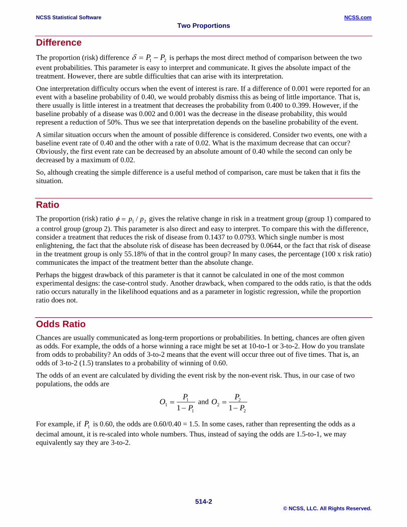
Difference The proportion (risk) difference 21 PP −=δ is perhaps the most direct method of comparison between the two event probabilities. This parameter is easy to interpret and communicate. It gives the absolute impact of the treatment. However, there are subtle difficulties that can arise with its interpretation.
One interpretation difficulty occurs when the event of interest is rare. If a difference of 0.001 were reported for an event with a baseline probability of 0.40, we would probably dismiss this as being of little importance. That is, there usually is little interest in a treatment that decreases the probability from 0.400 to 0.399. However, if the baseline probably of a disease was 0.002 and 0.001 was the decrease in the disease probability, this would represent a reduction of 50%. Thus we see that interpretation depends on the baseline probability of the event.
A similar situation occurs when the amount of possible difference is considered. Consider two events, one with a baseline event rate of 0.40 and the other with a rate of 0.02. What is the maximum decrease that can occur? Obviously, the first event rate can be decreased by an absolute amount of 0.40 while the second can only be decreased by a maximum of 0.02.
So, although creating the simple difference is a useful method of comparison, care must be taken that it fits the situation.
Ratio The proportion (risk) ratio 21 / pp=φ gives the relative change in risk in a treatment group (group 1) compared to a control group (group 2). This parameter is also direct and easy to interpret. To compare this with the difference, consider a treatment that reduces the risk of disease from 0.1437 to 0.0793. Which single number is most enlightening, the fact that the absolute risk of disease has been decreased by 0.0644, or the fact that risk of disease in the treatment group is only 55.18% of that in the control group? In many cases, the percentage (100 x risk ratio) communicates the impact of the treatment better than the absolute change.
Perhaps the biggest drawback of this parameter is that it cannot be calculated in one of the most common experimental designs: the case-control study. Another drawback, when compared to the odds ratio, is that the odds ratio occurs naturally in the likelihood equations and as a parameter in logistic regression, while the proportion ratio does not.
Odds Ratio Chances are usually communicated as long-term proportions or probabilities. In betting, chances are often given as odds. For example, the odds of a horse winning a race might be set at 10-to-1 or 3-to-2. How do you translate from odds to probability? An odds of 3-to-2 means that the event will occur three out of five times. That is, an odds of 3-to-2 (1.5) translates to a probability of winning of 0.60.
The odds of an event are calculated by dividing the event risk by the non-event risk. Thus, in our case of two populations, the odds are
1
11 1 P
PO−
= and 2
22 1 P
PO−
=
For example, if 1P is 0.60, the odds are 0.60/0.40 = 1.5. In some cases, rather than representing the odds as a decimal amount, it is re-scaled into whole numbers. Thus, instead of saying the odds are 1.5-to-1, we may equivalently say they are 3-to-2.

NCSS Statistical Software NCSS.com Two Proportions
514-3 © NCSS, LLC. All Rights Reserved.
In this context, the comparison of proportions may be done by comparing the odds through the ratio of the odds. The odds ratio of two events is
2
2
1
1
2
1
1
1
PP
PP
OO
−
−=
=ψ
Until one is accustomed to working with odds, the odds ratio is usually more difficult to interpret than the proportion (risk) ratio, but it is still the parameter of choice for many researchers. Reasons for this include the fact that the odds ratio can be accurately estimated from case-control studies, while the risk ratio cannot. Also, the odds ratio is the basis of logistic regression (used to study the influence of risk factors). Furthermore, the odds ratio is the natural parameter in the conditional likelihood of the two-group, binomial-response design. Finally, when the baseline event-rates are rare, the odds ratio provides a close approximation to the risk ratio since, in this case, 21 11 PP −≈− , so that
φψ =≈
−
−=
2
1
2
2
1
1
1
1PP
PP
PP
One benefit of the log of the odds ratio is its desirable statistical properties, such as its continuous range from negative infinity to positive infinity.
Confidence Intervals Both large sample and exact confidence intervals may be computed for the difference, the ratio, and the odds ratio.
Confidence Intervals for the Difference Several methods are available for computing a confidence interval of the difference between two proportions
21 PP −=δ . Newcombe (1998) conducted a comparative evaluation of eleven confidence interval methods. He recommended that the modified Wilson score method be used instead of the Pearson Chi-Square or the Yate’s Corrected Chi-Square. Beal (1987) found that the Score methods performed very well. The lower L and upper U limits of these intervals are computed as follows. Note that, unless otherwise stated, z z= α / 2 is the appropriate percentile from the standard normal distribution.
Cells with Zero Counts Extreme cases in which some cells are zero require special approaches with some of the tests given below. We have found that a simple solution that works well is to change the zeros to a small positive number such as 0.01. This produces the same results as other techniques of which we are aware.
NCSS Statistical Software NCSS.com Two Proportions
514-4 © NCSS, LLC. All Rights Reserved.
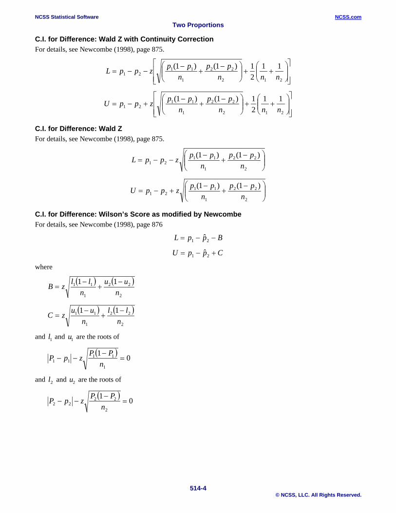
C.I. for Difference: Wald Z with Continuity Correction For details, see Newcombe (1998), page 875.
++
−+
−−−=
212
22
1
1121
1121)1()1(
nnnpp
nppzppL
++
−+
−+−=
212
22
1
1121
1121)1()1(
nnnpp
nppzppU
C.I. for Difference: Wald Z For details, see Newcombe (1998), page 875.
−+
−−−=
2
22
1
1121
)1()1(n
ppn
ppzppL
−+
−+−=
2
22
1
1121
)1()1(n
ppn
ppzppU
C.I. for Difference: Wilson’s Score as modified by Newcombe For details, see Newcombe (1998), page 876
BppL −−= 21 ˆ
CppU +−= 21 ˆ
where
( ) ( )2
22
1
11 11n
uun
llzB −+
−=
( ) ( )2
22
1
11 11n
lln
uuzC −+
−=
and l1 and u1 are the roots of
( ) 01
1
1111 =
−−−
nPPzpP
and l2 and u2 are the roots of
( ) 01
2
2222 =
−−−
nPPzpP
NCSS Statistical Software NCSS.com Two Proportions
514-5 © NCSS, LLC. All Rights Reserved.
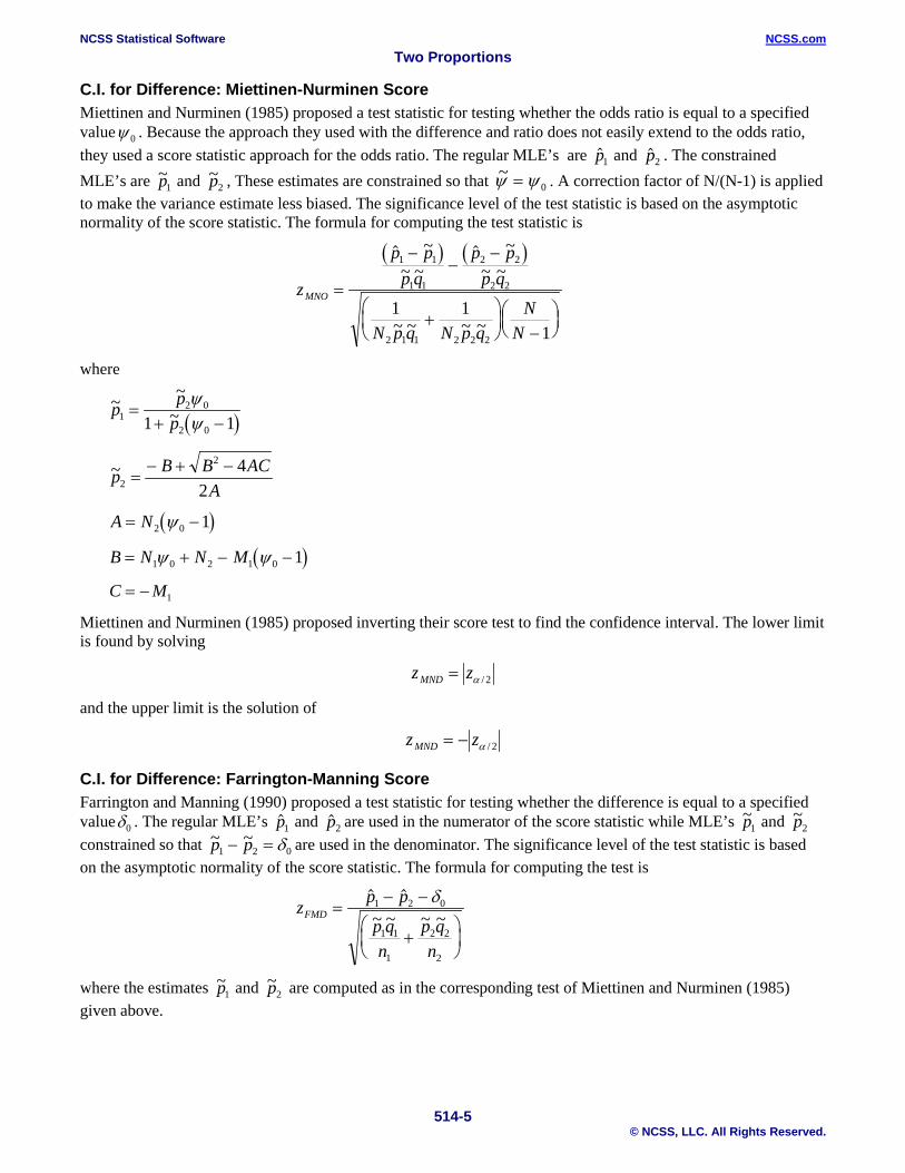
C.I. for Difference: Miettinen-Nurminen Score Miettinen and Nurminen (1985) proposed a test statistic for testing whether the odds ratio is equal to a specified valueψ 0 . Because the approach they used with the difference and ratio does not easily extend to the odds ratio, they used a score statistic approach for the odds ratio. The regular MLE’s are p1 and p2 . The constrained MLE’s are ~p1 and ~p2 , These estimates are constrained so that ~ψ ψ= 0 . A correction factor of N/(N-1) is applied to make the variance estimate less biased. The significance level of the test statistic is based on the asymptotic normality of the score statistic. The formula for computing the test statistic is
( ) ( )z
p pp q
p pp q
N p q N p qN
N
MNO =
−−
−
+
−
~~ ~
~~ ~
~ ~ ~ ~
1 1
1 1
2 2
2 2
2 1 1 2 2 2
1 11
where
( )~ ~
~p pp1
2 0
2 01 1=
+ −ψψ
~p B B ACA2
2 42
=− + −
( )A N= −2 0 1ψ
( )B N N M= + − −1 0 2 1 0 1ψ ψ
C M= − 1
Miettinen and Nurminen (1985) proposed inverting their score test to find the confidence interval. The lower limit is found by solving
z zMND = α / 2
and the upper limit is the solution of
z zMND = − α / 2
C.I. for Difference: Farrington-Manning Score Farrington and Manning (1990) proposed a test statistic for testing whether the difference is equal to a specified valueδ0 . The regular MLE’s p1 and p2 are used in the numerator of the score statistic while MLE’s ~p1 and ~p2 constrained so that ~ ~p p1 2 0− = δ are used in the denominator. The significance level of the test statistic is based on the asymptotic normality of the score statistic. The formula for computing the test is
z p p
p qn
p qn
FMD =− −
+
~ ~ ~ ~1 2 0
1 1
1
2 2
2
δ
where the estimates ~p1 and ~p2 are computed as in the corresponding test of Miettinen and Nurminen (1985) given above.
NCSS Statistical Software NCSS.com Two Proportions
514-6 © NCSS, LLC. All Rights Reserved.
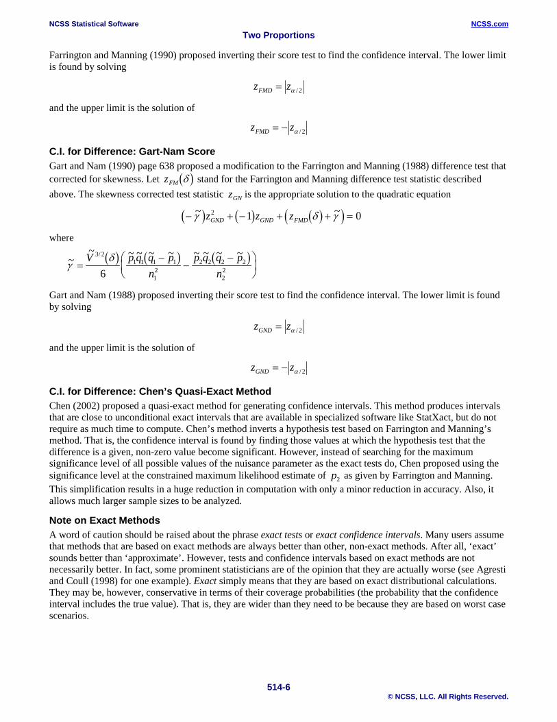
Farrington and Manning (1990) proposed inverting their score test to find the confidence interval. The lower limit is found by solving
z zFMD = α / 2
and the upper limit is the solution of
z zFMD = − α / 2
C.I. for Difference: Gart-Nam Score Gart and Nam (1990) page 638 proposed a modification to the Farrington and Manning (1988) difference test that corrected for skewness. Let ( )zFM δ stand for the Farrington and Manning difference test statistic described above. The skewness corrected test statistic zGN is the appropriate solution to the quadratic equation
( ) ( ) ( )( )− + − + + =~ ~γ δ γz z zGND GND FMD2 1 0
where
( ) ( ) ( )~~ ~ ~ ~ ~ ~ ~ ~ ~/
γδ
=−
−−
V p q q pn
p q q pn
3 21 1 1 1
12
2 2 2 2
226
Gart and Nam (1988) proposed inverting their score test to find the confidence interval. The lower limit is found by solving
z zGND = α / 2
and the upper limit is the solution of
z zGND = − α / 2
C.I. for Difference: Chen’s Quasi-Exact Method Chen (2002) proposed a quasi-exact method for generating confidence intervals. This method produces intervals that are close to unconditional exact intervals that are available in specialized software like StatXact, but do not require as much time to compute. Chen’s method inverts a hypothesis test based on Farrington and Manning’s method. That is, the confidence interval is found by finding those values at which the hypothesis test that the difference is a given, non-zero value become significant. However, instead of searching for the maximum significance level of all possible values of the nuisance parameter as the exact tests do, Chen proposed using the significance level at the constrained maximum likelihood estimate of p2 as given by Farrington and Manning. This simplification results in a huge reduction in computation with only a minor reduction in accuracy. Also, it allows much larger sample sizes to be analyzed.
Note on Exact Methods A word of caution should be raised about the phrase exact tests or exact confidence intervals. Many users assume that methods that are based on exact methods are always better than other, non-exact methods. After all, ‘exact’ sounds better than ‘approximate’. However, tests and confidence intervals based on exact methods are not necessarily better. In fact, some prominent statisticians are of the opinion that they are actually worse (see Agresti and Coull (1998) for one example). Exact simply means that they are based on exact distributional calculations. They may be, however, conservative in terms of their coverage probabilities (the probability that the confidence interval includes the true value). That is, they are wider than they need to be because they are based on worst case scenarios.
NCSS Statistical Software NCSS.com Two Proportions
514-7 © NCSS, LLC. All Rights Reserved.
Confidence Intervals for the Ratio
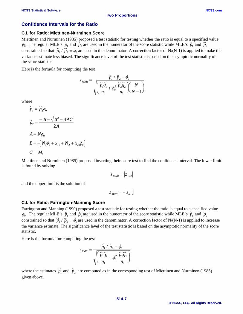
C.I. for Ratio: Miettinen-Nurminen Score Miettinen and Nurminen (1985) proposed a test statistic for testing whether the ratio is equal to a specified valueφ0 . The regular MLE’s p1 and p2 are used in the numerator of the score statistic while MLE’s ~p1 and ~p2 constrained so that ~ / ~p p1 2 0= φ are used in the denominator. A correction factor of N/(N-1) is applied to make the variance estimate less biased. The significance level of the test statistic is based on the asymptotic normality of the score statistic.
Here is the formula for computing the test
z p p
p qn
p qn
NN
MNR =−
+
−
/ ~ ~ ~ ~
1 2 0
1 1
102 2 2
2 1
φ
φ
where ~ ~p p1 2 0= φ
~p B B ACA2
2 42
=− − −
A N= φ0
[ ]B N x N x= − + + +1 0 11 2 21 0φ φ C M= 1
Miettinen and Nurminen (1985) proposed inverting their score test to find the confidence interval. The lower limit is found by solving
z zMNR = α / 2
and the upper limit is the solution of
z zMNR = − α / 2
C.I. for Ratio: Farrington-Manning Score Farrington and Manning (1990) proposed a test statistic for testing whether the ratio is equal to a specified valueφ0 . The regular MLE’s p1 and p2 are used in the numerator of the score statistic while MLE’s ~p1 and ~p2 constrained so that ~ / ~p p1 2 0= φ are used in the denominator. A correction factor of N/(N-1) is applied to increase the variance estimate. The significance level of the test statistic is based on the asymptotic normality of the score statistic.
Here is the formula for computing the test
z p p
p qn
p qn
FMR =−
+
/ ~ ~ ~ ~
1 2 0
1 1
102 2 2
2
φ
φ
where the estimates ~p1 and ~p2 are computed as in the corresponding test of Miettinen and Nurminen (1985) given above.
NCSS Statistical Software NCSS.com Two Proportions
514-8 © NCSS, LLC. All Rights Reserved.
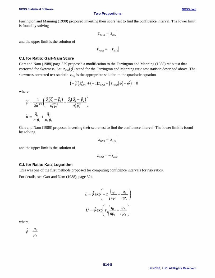
Farrington and Manning (1990) proposed inverting their score test to find the confidence interval. The lower limit is found by solving
z zFMR = α / 2
and the upper limit is the solution of
z zFMR = − α / 2
C.I. for Ratio: Gart-Nam Score Gart and Nam (1988) page 329 proposed a modification to the Farrington and Manning (1988) ratio test that corrected for skewness. Let ( )zFM φ stand for the Farrington and Manning ratio test statistic described above. The skewness corrected test statistic zGN is the appropriate solution to the quadratic equation
( ) ( ) ( )( )− + − + + =~ ~ϕ φ ϕz z zGNR GNR FMR2 1 0
where
( ) ( )~~
~ ~ ~~
~ ~ ~~/ϕ =
−−
−
16 3 2
1 1 1
12
12
2 2 2
22
22u
q q pn p
q q pn p
~ ~~
~~u q
n pq
n p= +1
1 1
2
2 2 Gart and Nam (1988) proposed inverting their score test to find the confidence interval. The lower limit is found by solving
z zGNR = α / 2
and the upper limit is the solution of
z zGNR = − α / 2
C.I. for Ratio: Katz Logarithm This was one of the first methods proposed for computing confidence intervals for risk ratios.
For details, see Gart and Nam (1988), page 324.
+−=
2
2
1
1expˆnpq
npqzL φ
+=
2
2
1
1expˆnpq
npqzU φ
where
2
1ˆpp
=φ
NCSS Statistical Software NCSS.com Two Proportions
514-9 © NCSS, LLC. All Rights Reserved.
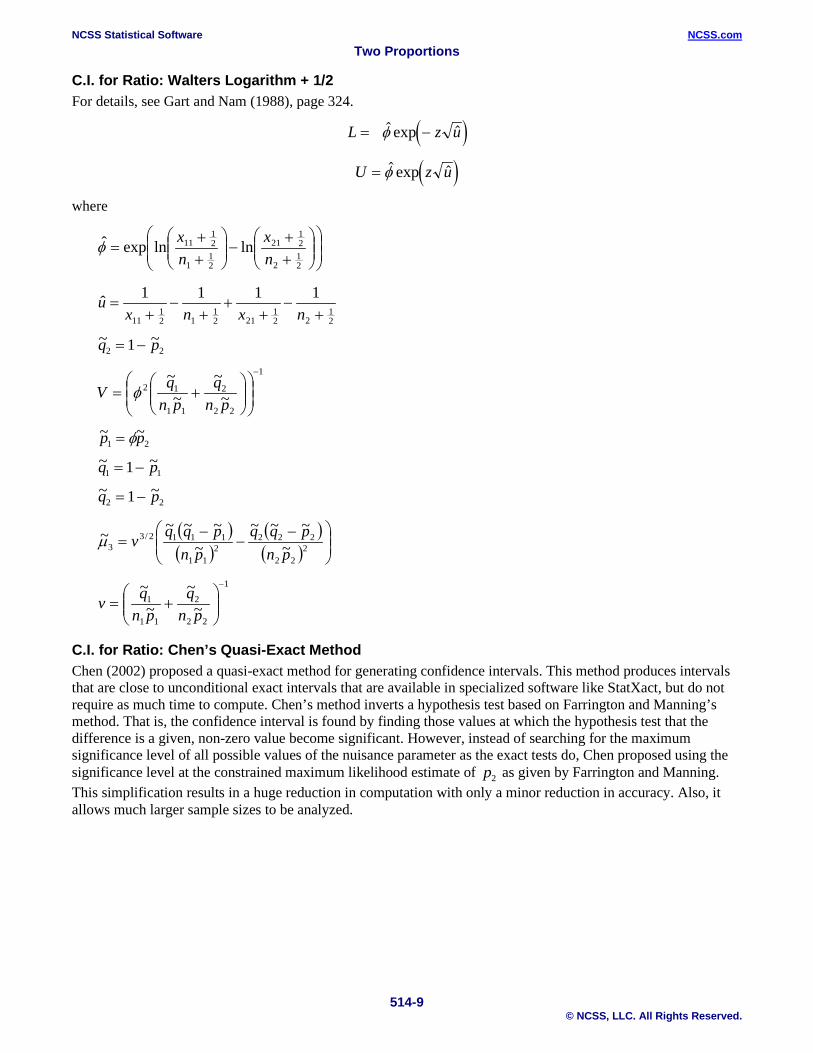
C.I. for Ratio: Walters Logarithm + 1/2 For details, see Gart and Nam (1988), page 324.
( )L z u= − exp φ
( )U z u= exp φ
where
++
−
++
=21
2
21
21
21
1
21
11 lnlnexpˆnx
nxφ
21
221
2121
121
11
1111ˆ+
−+
++
−+
=nxnx
u
~ ~q p2 21= − 1
22
2
11
12~
~~
~ −
+=
pnq
pnqV φ
~ ~p p1 2= φ ~ ~q p1 11= − ~ ~q p2 21= −
( )( )
( )( )
−−
−= 2
22
2222
11
1112/33 ~
~~~~
~~~~pn
pqqpn
pqqvµ
1
22
2
11
1~
~~
~ −
+=
pnq
pnqv
C.I. for Ratio: Chen’s Quasi-Exact Method Chen (2002) proposed a quasi-exact method for generating confidence intervals. This method produces intervals that are close to unconditional exact intervals that are available in specialized software like StatXact, but do not require as much time to compute. Chen’s method inverts a hypothesis test based on Farrington and Manning’s method. That is, the confidence interval is found by finding those values at which the hypothesis test that the difference is a given, non-zero value become significant. However, instead of searching for the maximum significance level of all possible values of the nuisance parameter as the exact tests do, Chen proposed using the significance level at the constrained maximum likelihood estimate of p2 as given by Farrington and Manning. This simplification results in a huge reduction in computation with only a minor reduction in accuracy. Also, it allows much larger sample sizes to be analyzed.
NCSS Statistical Software NCSS.com Two Proportions
514-10 © NCSS, LLC. All Rights Reserved.
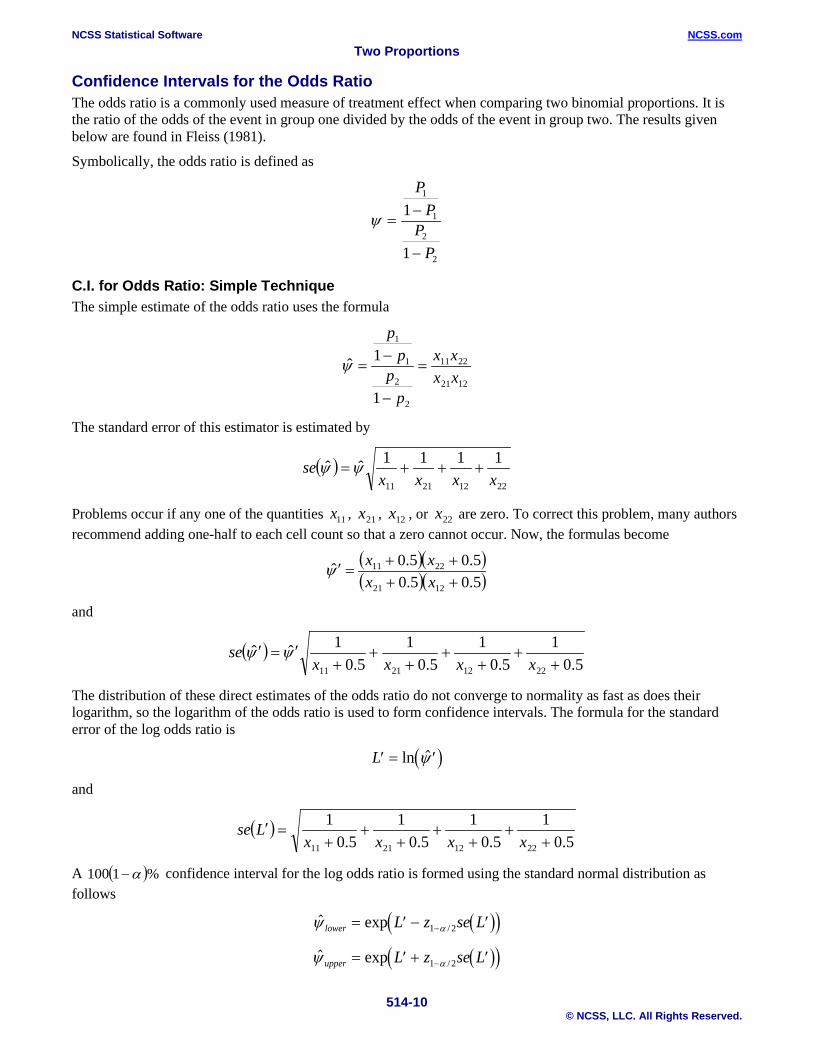
Confidence Intervals for the Odds Ratio The odds ratio is a commonly used measure of treatment effect when comparing two binomial proportions. It is the ratio of the odds of the event in group one divided by the odds of the event in group two. The results given below are found in Fleiss (1981).
Symbolically, the odds ratio is defined as
2
2
1
1
1
1
PP
PP
−
−=ψ
C.I. for Odds Ratio: Simple Technique The simple estimate of the odds ratio uses the formula
1221
2211
2
2
1
1
1
1ˆxxxx
pp
pp
=
−
−=ψ
The standard error of this estimator is estimated by
( )22122111
1111ˆˆxxxx
se +++=ψψ
Problems occur if any one of the quantities 11x , 21x , 12x , or 22x are zero. To correct this problem, many authors recommend adding one-half to each cell count so that a zero cannot occur. Now, the formulas become
( )( )( )( )5.05.0
5.05.0ˆ1221
2211
++++
=′xxxxψ
and
( )5.0
15.0
15.0
15.0
1ˆˆ22122111 +
++
++
++
′=′xxxx
se ψψ
The distribution of these direct estimates of the odds ratio do not converge to normality as fast as does their logarithm, so the logarithm of the odds ratio is used to form confidence intervals. The formula for the standard error of the log odds ratio is
( )′ = ′L ln ψ
and
( )5.0
15.0
15.0
15.0
122122111 +
++
++
++
=′xxxx
Lse
A ( )%1100 α− confidence interval for the log odds ratio is formed using the standard normal distribution as follows
( )( ) exp /ψ αlower L z se L= ′ − ′−1 2
( )( ) exp /ψ αupper L z se L= ′ + ′−1 2
NCSS Statistical Software NCSS.com Two Proportions
514-11 © NCSS, LLC. All Rights Reserved.
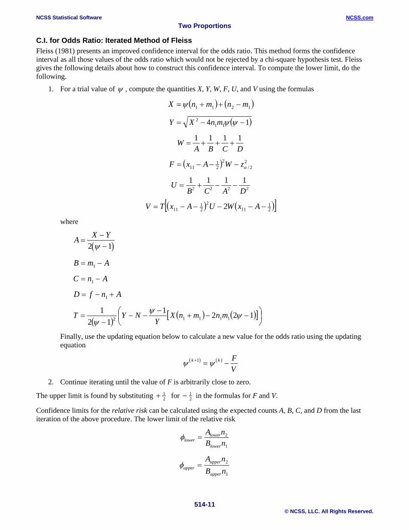
C.I. for Odds Ratio: Iterated Method of Fleiss Fleiss (1981) presents an improved confidence interval for the odds ratio. This method forms the confidence interval as all those values of the odds ratio which would not be rejected by a chi-square hypothesis test. Fleiss gives the following details about how to construct this confidence interval. To compute the lower limit, do the following.
1. For a trial value of ψ , compute the quantities X, Y, W, F, U, and V using the formulas
( ) ( )1211 mnmnX −++=ψ
( )14 112 −−= ψψmnXY
WA B C D
= + + +1 1 1 1
( ) 22/
221
11 αzWAxF −−−=
UB C A D
= + − −1 1 1 1
2 2 2 2
( ) ( )[ ]21
112
21
11 2 −−−−−= AxWUAxTV
where
( )A X Y=
−−2 1ψ
AmB −= 1
AnC −= 1
AnfD +−= 1
( )( ) ( )[ ]
−−+
−−−
−= 1221
121
11112 ψψψ
mnmnXY
NYT
Finally, use the updating equation below to calculate a new value for the odds ratio using the updating equation
( ) ( )ψ ψk k FV
+ = −1
2. Continue iterating until the value of F is arbitrarily close to zero.
The upper limit is found by substituting + 12 for − 1
2 in the formulas for F and V.
Confidence limits for the relative risk can be calculated using the expected counts A, B, C, and D from the last iteration of the above procedure. The lower limit of the relative risk
1
2
nBnA
lower
lowerlower =φ
1
2
nBnA
upper
upperupper =φ
NCSS Statistical Software NCSS.com Two Proportions
514-12 © NCSS, LLC. All Rights Reserved.
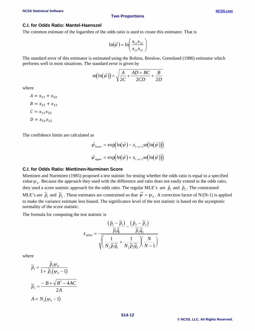
C.I. for Odds Ratio: Mantel-Haenszel The common estimate of the logarithm of the odds ratio is used to create this estimator. That is
( )
=
1221
2211lnˆlnxxxxψ
The standard error of this estimator is estimated using the Robins, Breslow, Greenland (1986) estimator which performs well in most situations. The standard error is given by
( )( )se ln ψ = ++
+AC
AD BCCD
BD2 2 2
where
𝐴𝐴 = 𝑥𝑥11 + 𝑥𝑥22
𝐵𝐵 = 𝑥𝑥21 + 𝑥𝑥12
𝐶𝐶 = 𝑥𝑥11𝑥𝑥22
𝐷𝐷 = 𝑥𝑥21𝑥𝑥12
The confidence limits are calculated as
( ) ( )( )( ) exp ln ln /ψ ψ ψαlower z se= − −1 2
( ) ( )( )( ) exp ln ln /ψ ψ ψαupper z se= + −1 2
C.I. for Odds Ratio: Miettinen-Nurminen Score Miettinen and Nurminen (1985) proposed a test statistic for testing whether the odds ratio is equal to a specified valueψ 0 . Because the approach they used with the difference and ratio does not easily extend to the odds ratio, they used a score statistic approach for the odds ratio. The regular MLE’s are p1 and p2 . The constrained MLE’s are ~p1 and ~p2 . These estimates are constrained so that ~ψ ψ= 0 . A correction factor of N/(N-1) is applied to make the variance estimate less biased. The significance level of the test statistic is based on the asymptotic normality of the score statistic.
The formula for computing the test statistic is
( ) ( )z
p pp q
p pp q
N p q N p qN
N
MNO =
−−
−
+
−
~~ ~
~~ ~
~ ~ ~ ~
1 1
1 1
2 2
2 2
2 1 1 2 2 2
1 11
where
( )~ ~
~p pp1
2 0
2 01 1=
+ −ψψ
~p B B ACA2
2 42
=− + −
( )A N= −2 0 1ψ
NCSS Statistical Software NCSS.com Two Proportions
514-13 © NCSS, LLC. All Rights Reserved.
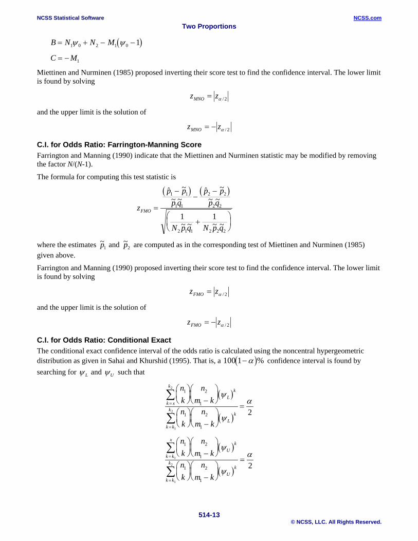
( )B N N M= + − −1 0 2 1 0 1ψ ψ
C M= − 1
Miettinen and Nurminen (1985) proposed inverting their score test to find the confidence interval. The lower limit is found by solving
2/αzzMNO =
and the upper limit is the solution of
2/αzzMNO −=
C.I. for Odds Ratio: Farrington-Manning Score Farrington and Manning (1990) indicate that the Miettinen and Nurminen statistic may be modified by removing the factor N/(N-1).
The formula for computing this test statistic is
( ) ( )z
p pp q
p pp q
N p q N p q
FMO =
−−
−
+
~~ ~
~~ ~
~ ~ ~ ~
1 1
1 1
2 2
2 2
2 1 1 2 2 2
1 1
where the estimates ~p1 and ~p2 are computed as in the corresponding test of Miettinen and Nurminen (1985) given above.
Farrington and Manning (1990) proposed inverting their score test to find the confidence interval. The lower limit is found by solving
2/αzzFMO =
and the upper limit is the solution of
2/αzzFMO −=
C.I. for Odds Ratio: Conditional Exact The conditional exact confidence interval of the odds ratio is calculated using the noncentral hypergeometric distribution as given in Sahai and Khurshid (1995). That is, a ( )100 1−α % confidence interval is found by searching for ψ L and ψU such that
( )
( )
nk
nm k
nk
nm k
Lk
k x
k
Lk
k k
k
1 2
1
1 2
1
2
1
2 2
−
−
==
=
∑
∑
ψ
ψ
α
( )
( )
nk
nm k
nk
nm k
Uk
k k
x
Uk
k k
k
1 2
1
1 2
1
1
1
2 2
−
−
==
=
∑
∑
ψ
ψ
α
NCSS Statistical Software NCSS.com Two Proportions
514-14 © NCSS, LLC. All Rights Reserved.
where
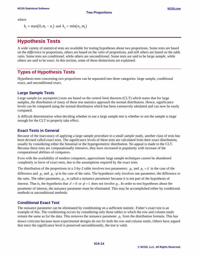
and ( )k n m2 1 1= min ,
Hypothesis Tests A wide variety of statistical tests are available for testing hypotheses about two proportions. Some tests are based on the difference in proportions, others are based on the ratio of proportions, and still others are based on the odds ratio. Some tests are conditional, while others are unconditional. Some tests are said to be large sample, while others are said to be exact. In this section, some of these distinctions are explained.
Types of Hypothesis Tests Hypothesis tests concerning two proportions can be separated into three categories: large sample, conditional exact, and unconditional exact.
Large Sample Tests Large sample (or asymptotic) tests are based on the central limit theorem (CLT) which states that for large samples, the distribution of many of these test statistics approach the normal distribution. Hence, significance levels can be computed using the normal distribution which has been extensively tabulated and can now be easily computed.
A difficult determination when deciding whether to use a large sample test is whether or not the sample is large enough for the CLT to properly take effect.
Exact Tests in General Because of the inaccuracy of applying a large sample procedure to a small sample study, another class of tests has been devised called exact tests. The significance levels of these tests are calculated from their exact distribution, usually by considering either the binomial or the hypergeometric distribution. No appeal is made to the CLT. Because these tests are computationally intensive, they have increased in popularity with increase of the computational abilities of computers.
Even with the availability of modern computers, approximate large sample techniques cannot be abandoned completely in favor of exact tests, due to the assumptions required by the exact tests.
The distribution of the proportions in a 2-by-2 table involves two parameters: 1p and δ+1p in the case of the difference and 1p and φ/1p in the case of the ratio. The hypothesis only involves one parameter, the difference or the ratio. The other parameter, 1p , is called a nuisance parameter because it is not part of the hypothesis of interest. That is, the hypothesis that 0=δ or 1=φ does not involve 1p . In order to test hypotheses about the parameter of interest, the nuisance parameter must be eliminated. This may be accomplished either by conditional methods or unconditional methods.
Conditional Exact Test The nuisance parameter can be eliminated by conditioning on a sufficient statistic. Fisher’s exact test is an example of this. The conditioning occurs by considering only those tables in which the row and column totals remain the same as for the data. This removes the nuisance parameter 1p from the distribution formula. This has drawn criticism because most experimental designs do not fix both the row and column totals. Others have argued that since the significance level is preserved unconditionally, the test is valid.
( )k m n1 1 10= −max ,
NCSS Statistical Software NCSS.com Two Proportions
514-15 © NCSS, LLC. All Rights Reserved.
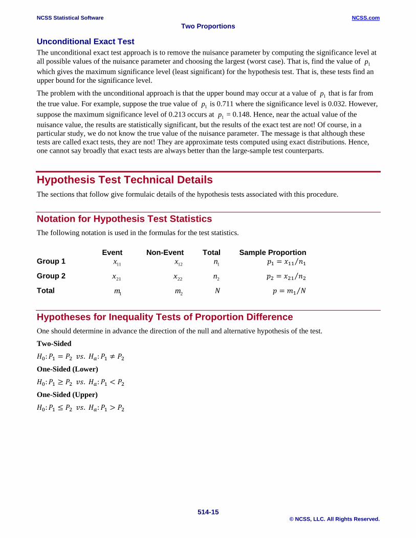
Unconditional Exact Test The unconditional exact test approach is to remove the nuisance parameter by computing the significance level at all possible values of the nuisance parameter and choosing the largest (worst case). That is, find the value of 1p which gives the maximum significance level (least significant) for the hypothesis test. That is, these tests find an upper bound for the significance level.
The problem with the unconditional approach is that the upper bound may occur at a value of 1p that is far from the true value. For example, suppose the true value of 1p is 0.711 where the significance level is 0.032. However, suppose the maximum significance level of 0.213 occurs at 1p = 0.148. Hence, near the actual value of the nuisance value, the results are statistically significant, but the results of the exact test are not! Of course, in a particular study, we do not know the true value of the nuisance parameter. The message is that although these tests are called exact tests, they are not! They are approximate tests computed using exact distributions. Hence, one cannot say broadly that exact tests are always better than the large-sample test counterparts.
Hypothesis Test Technical Details The sections that follow give formulaic details of the hypothesis tests associated with this procedure.
Notation for Hypothesis Test Statistics The following notation is used in the formulas for the test statistics.
Event Non-Event Total Sample Proportion Group 1 x11 x12 n1 𝑝𝑝1 = 𝑥𝑥11 𝑛𝑛1⁄
Group 2 x21 x22 n2 𝑝𝑝2 = 𝑥𝑥21 𝑛𝑛2⁄
Total m1 m2 𝑁𝑁 𝑝𝑝 = 𝑚𝑚1 𝑁𝑁⁄
Hypotheses for Inequality Tests of Proportion Difference One should determine in advance the direction of the null and alternative hypothesis of the test.
Two-Sided
𝐻𝐻0:𝑃𝑃1 = 𝑃𝑃2 𝑣𝑣𝑣𝑣. 𝐻𝐻𝑎𝑎:𝑃𝑃1 ≠ 𝑃𝑃2
One-Sided (Lower)
𝐻𝐻0:𝑃𝑃1 ≥ 𝑃𝑃2 𝑣𝑣𝑣𝑣. 𝐻𝐻𝑎𝑎:𝑃𝑃1 < 𝑃𝑃2
One-Sided (Upper)
𝐻𝐻0:𝑃𝑃1 ≤ 𝑃𝑃2 𝑣𝑣𝑣𝑣. 𝐻𝐻𝑎𝑎:𝑃𝑃1 > 𝑃𝑃2
NCSS Statistical Software NCSS.com Two Proportions
514-16 © NCSS, LLC. All Rights Reserved.
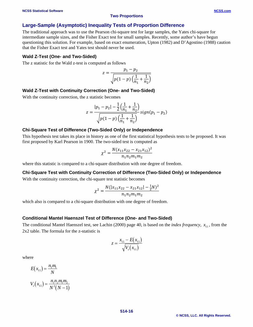
Large-Sample (Asymptotic) Inequality Tests of Proportion Difference The traditional approach was to use the Pearson chi-square test for large samples, the Yates chi-square for intermediate sample sizes, and the Fisher Exact test for small samples. Recently, some author’s have begun questioning this solution. For example, based on exact enumeration, Upton (1982) and D’Agostino (1988) caution that the Fisher Exact test and Yates test should never be used.
Wald Z-Test (One- and Two-Sided) The z statistic for the Wald z-test is computed as follows
𝑧𝑧 =𝑝𝑝1 − 𝑝𝑝2
𝑝𝑝(1 − 𝑝𝑝) 1𝑛𝑛1
+ 1𝑛𝑛2
Wald Z-Test with Continuity Correction (One- and Two-Sided) With the continuity correction, the z statistic becomes
𝑧𝑧 =|𝑝𝑝1 − 𝑝𝑝2| − 1
2 1𝑛𝑛1
+ 1𝑛𝑛2
𝑝𝑝(1 − 𝑝𝑝) 1𝑛𝑛1
+ 1𝑛𝑛2𝑣𝑣𝑠𝑠𝑠𝑠𝑛𝑛(𝑝𝑝1 − 𝑝𝑝2)
Chi-Square Test of Difference (Two-Sided Only) or Independence This hypothesis test takes its place in history as one of the first statistical hypothesis tests to be proposed. It was first proposed by Karl Pearson in 1900. The two-sided test is computed as
𝜒𝜒2 =𝑁𝑁(𝑥𝑥11𝑥𝑥22 − 𝑥𝑥21𝑥𝑥12)2
𝑛𝑛1𝑛𝑛2𝑚𝑚1𝑚𝑚2
where this statistic is compared to a chi-square distribution with one degree of freedom.
Chi-Square Test with Continuity Correction of Difference (Two-Sided Only) or Independence With the continuity correction, the chi-square test statistic becomes
𝜒𝜒2 =𝑁𝑁(|𝑥𝑥11𝑥𝑥22 − 𝑥𝑥21𝑥𝑥12|− 1
2𝑁𝑁)2
𝑛𝑛1𝑛𝑛2𝑚𝑚1𝑚𝑚2
which also is compared to a chi-square distribution with one degree of freedom.
Conditional Mantel Haenszel Test of Difference (One- and Two-Sided) The conditional Mantel Haenszel test, see Lachin (2000) page 40, is based on the index frequency, x11 , from the 2x2 table. The formula for the z-statistic is
( )( )
zx E x
V xc
=−11 11
11
where
( )E x n mN111 1=
( ) ( )V x n n m m
N Nc 111 2 1 22 1
=−
NCSS Statistical Software NCSS.com Two Proportions
514-17 © NCSS, LLC. All Rights Reserved.
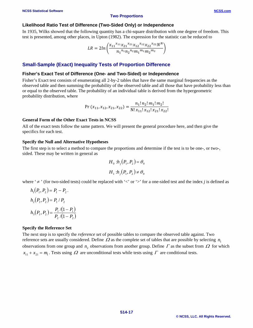
Likelihood Ratio Test of Difference (Two-Sided Only) or Independence In 1935, Wilks showed that the following quantity has a chi-square distribution with one degree of freedom. This test is presented, among other places, in Upton (1982). The expression for the statistic can be reduced to
𝐿𝐿𝐿𝐿 = 2𝑙𝑙𝑛𝑛 𝑥𝑥11𝑥𝑥11𝑥𝑥21𝑥𝑥21𝑥𝑥12𝑥𝑥12𝑥𝑥22𝑥𝑥22𝑁𝑁𝑁𝑁
𝑛𝑛1𝑛𝑛1𝑛𝑛2𝑛𝑛2𝑚𝑚1𝑚𝑚1𝑚𝑚2
𝑚𝑚2
Small-Sample (Exact) Inequality Tests of Proportion Difference
Fisher’s Exact Test of Difference (One- and Two-Sided) or Independence Fisher’s Exact test consists of enumerating all 2-by-2 tables that have the same marginal frequencies as the observed table and then summing the probability of the observed table and all those that have probability less than or equal to the observed table. The probability of an individual table is derived from the hypergeometric probability distribution, where
Pr (𝑥𝑥11,𝑥𝑥12, 𝑥𝑥21,𝑥𝑥22) =𝑛𝑛1!𝑛𝑛2!𝑚𝑚1!𝑚𝑚2!
N! 𝑥𝑥11! 𝑥𝑥12!𝑥𝑥21!𝑥𝑥22!
General Form of the Other Exact Tests in NCSS All of the exact tests follow the same pattern. We will present the general procedure here, and then give the specifics for each test.
Specify the Null and Alternative Hypotheses The first step is to select a method to compare the proportions and determine if the test is to be one-, or two-, sided. These may be written in general as
( ) 0210 ,: θ=PPhH j
( ) 0211 ,: θ≠PPhH j
where ‘≠ ’ (for two-sided tests) could be replaced with ‘<’ or ‘>’ for a one-sided test and the index j is defined as
( ) 21211 , PPPPh −= .
( ) 21212 /, PPPPh =
( ) ( )( )22
11213 1/
1/,PPPPPPh
−−
=
Specify the Reference Set The next step is to specify the reference set of possible tables to compare the observed table against. Two reference sets are usually considered. Define Ω as the complete set of tables that are possible by selecting n1 observations from one group and n2 observations from another group. Define Γ as the subset from Ω for which x x m11 21 1+ = . Tests using Ω are unconditional tests while tests using Γ are conditional tests.
NCSS Statistical Software NCSS.com Two Proportions
514-18 © NCSS, LLC. All Rights Reserved.
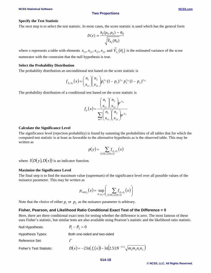
Specify the Test Statistic The next step is to select the test statistic. In most cases, the score statistic is used which has the general form
𝐷𝐷(𝑥𝑥) =ℎ𝑗𝑗(𝑝𝑝1,𝑝𝑝2) − 𝜃𝜃0
𝑉𝑉ℎ𝑗𝑗(𝜃𝜃0)
where x represents a table with elements 22211211 ,,, xxxx and ( )~Vh jθ0 is the estimated variance of the score
numerator with the constraint that the null hypothesis is true.
Select the Probability Distribution The probability distribution an unconditional test based on the score statistic is
( ) 22211211
21)1()1( 2211
21
2
11
1,
xxxxpp pppp
xn
xn
xf −−
=
The probability distribution of a conditional test based on the score statistic is
( )∑
Γ∈
=
x
x
x
xn
xn
xn
xn
xf11
11
21
2
11
1
21
2
11
1
ψ
ψ
ψ
Calculate the Significance Level The significance level (rejection probability) is found by summing the probabilities of all tables that for which the computed test statistic is at least as favorable to the alternative hypothesis as is the observed table. This may be written as
( ) ( )( ) ( )( )∑=
xDyDIpp xfyp
,, 21
where ( ) ( )( )xDyDI , is an indicator function.
Maximize the Significance Level The final step is to find the maximum value (supremum) of the significance level over all possible values of the nuisance parameter. This may be written as
( ) ( )( ) ( )( )
= ∑
<< xDyDIpp
pp xfxp
,,
10sup 21
22
sup
Note that the choice of either p1 or p2 as the nuisance parameter is arbitrary.
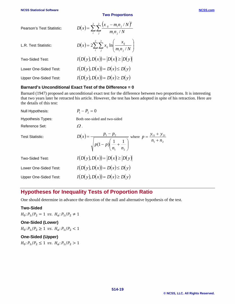
Fisher, Pearson, and Likelihood Ratio Conditional Exact Test of the Difference = 0 Here, there are three conditional exact tests for testing whether the difference is zero. The most famous of these uses Fisher’s statistic, but similar tests are also available using Pearson’s statistic and the likelihood ratio statistic.
Null Hypothesis: 021 =− PP
Hypothesis Types: Both one-sided and two-sided
Reference Set: Γ
Fisher’s Test Statistic: ( ) ( )( ) ( )21212/3
1 51.2lnln2 nnmmNxfxD −−−=
NCSS Statistical Software NCSS.com Two Proportions
514-19 © NCSS, LLC. All Rights Reserved.
Pearson’s Test Statistic: ( ) ( )∑∑
−=
2 2 2
//
i j ji
jiij
NnmNnmx
xD
L.R. Test Statistic: ( ) ∑∑
=
2 2
/ln2
i j ji
ijij Nnm
xxxD
Two-Sided Test: ( ) ( )( ) ( ) ( )yDxDxDyDI ≥=,
Lower One-Sided Test: ( ) ( )( ) ( ) ( )yDxDxDyDI ≤=,
Upper One-Sided Test: ( ) ( )( ) ( ) ( )yDxDxDyDI ≥=,
Barnard’s Unconditional Exact Test of the Difference = 0 Barnard (1947) proposed an unconditional exact test for the difference between two proportions. It is interesting that two years later he retracted his article. However, the test has been adopted in spite of his retraction. Here are the details of this test:
Null Hypothesis: 021 =− PP
Hypothesis Types: Both one-sided and two-sided
Reference Set: Ω .
Test Statistic: ( )
+−
−=
21
21
11)1(nn
pp
ppxD where 21
2111
nnyyp
++
=
Two-Sided Test: ( ) ( )( ) ( ) ( )yDxDxDyDI ≥=,
Lower One-Sided Test: ( ) ( )( ) ( ) ( )yDxDxDyDI ≤=,
Upper One-Sided Test: ( ) ( )( ) ( ) ( )yDxDxDyDI ≥=,
Hypotheses for Inequality Tests of Proportion Ratio One should determine in advance the direction of the null and alternative hypothesis of the test.
Two-Sided 𝐻𝐻0:𝑃𝑃1/𝑃𝑃2 = 1 𝑣𝑣𝑣𝑣. 𝐻𝐻𝑎𝑎:𝑃𝑃1/𝑃𝑃2 ≠ 1
One-Sided (Lower) 𝐻𝐻0:𝑃𝑃1/𝑃𝑃2 ≥ 1 𝑣𝑣𝑣𝑣. 𝐻𝐻𝑎𝑎:𝑃𝑃1/𝑃𝑃2 < 1
One-Sided (Upper) 𝐻𝐻0:𝑃𝑃1/𝑃𝑃2 ≤ 1 𝑣𝑣𝑣𝑣. 𝐻𝐻𝑎𝑎:𝑃𝑃1/𝑃𝑃2 > 1
NCSS Statistical Software NCSS.com Two Proportions
514-20 © NCSS, LLC. All Rights Reserved.
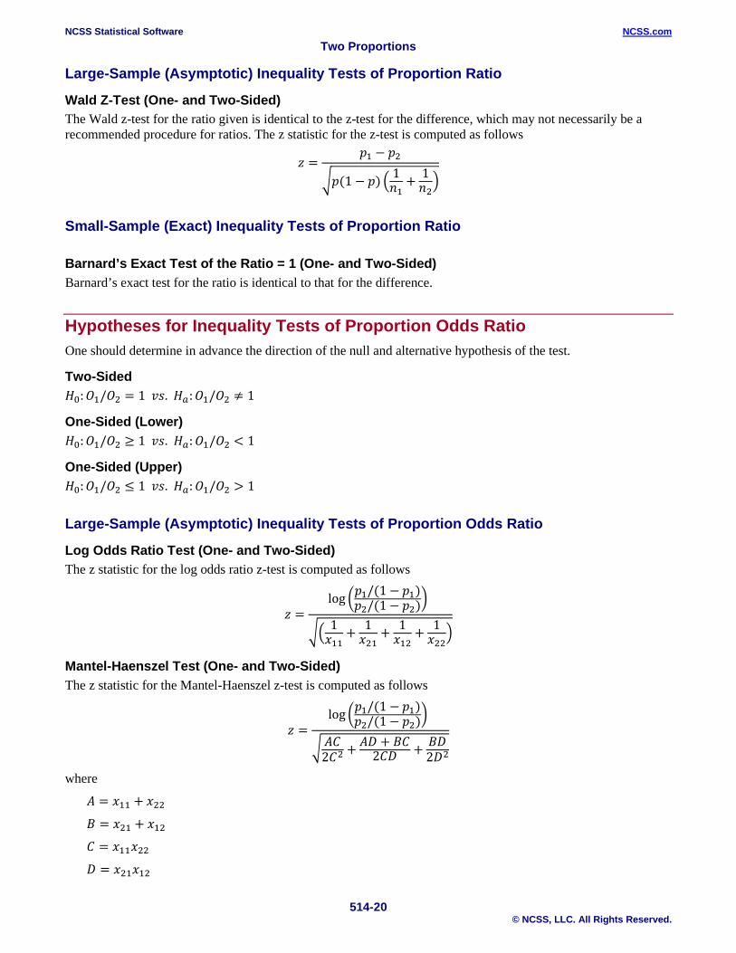
Large-Sample (Asymptotic) Inequality Tests of Proportion Ratio
Wald Z-Test (One- and Two-Sided) The Wald z-test for the ratio given is identical to the z-test for the difference, which may not necessarily be a recommended procedure for ratios. The z statistic for the z-test is computed as follows
𝑧𝑧 =𝑝𝑝1 − 𝑝𝑝2
𝑝𝑝(1 − 𝑝𝑝) 1𝑛𝑛1
+ 1𝑛𝑛2
Small-Sample (Exact) Inequality Tests of Proportion Ratio
Barnard’s Exact Test of the Ratio = 1 (One- and Two-Sided) Barnard’s exact test for the ratio is identical to that for the difference.
Hypotheses for Inequality Tests of Proportion Odds Ratio One should determine in advance the direction of the null and alternative hypothesis of the test.
Two-Sided 𝐻𝐻0:𝑂𝑂1/𝑂𝑂2 = 1 𝑣𝑣𝑣𝑣. 𝐻𝐻𝑎𝑎:𝑂𝑂1/𝑂𝑂2 ≠ 1
One-Sided (Lower) 𝐻𝐻0:𝑂𝑂1/𝑂𝑂2 ≥ 1 𝑣𝑣𝑣𝑣. 𝐻𝐻𝑎𝑎:𝑂𝑂1/𝑂𝑂2 < 1
One-Sided (Upper) 𝐻𝐻0:𝑂𝑂1/𝑂𝑂2 ≤ 1 𝑣𝑣𝑣𝑣. 𝐻𝐻𝑎𝑎:𝑂𝑂1/𝑂𝑂2 > 1
Large-Sample (Asymptotic) Inequality Tests of Proportion Odds Ratio
Log Odds Ratio Test (One- and Two-Sided) The z statistic for the log odds ratio z-test is computed as follows
𝑧𝑧 =log 𝑝𝑝1/(1 − 𝑝𝑝1)
𝑝𝑝2/(1 − 𝑝𝑝2)
1𝑥𝑥11
+ 1𝑥𝑥21
+ 1𝑥𝑥12
+ 1𝑥𝑥22
Mantel-Haenszel Test (One- and Two-Sided) The z statistic for the Mantel-Haenszel z-test is computed as follows
𝑧𝑧 =log 𝑝𝑝1/(1 − 𝑝𝑝1)
𝑝𝑝2/(1 − 𝑝𝑝2)
𝐴𝐴𝐶𝐶2𝐶𝐶2 + 𝐴𝐴𝐷𝐷 + 𝐵𝐵𝐶𝐶
2𝐶𝐶𝐷𝐷 + 𝐵𝐵𝐷𝐷2𝐷𝐷2
where
𝐴𝐴 = 𝑥𝑥11 + 𝑥𝑥22
𝐵𝐵 = 𝑥𝑥21 + 𝑥𝑥12
𝐶𝐶 = 𝑥𝑥11𝑥𝑥22
𝐷𝐷 = 𝑥𝑥21𝑥𝑥12
NCSS Statistical Software NCSS.com Two Proportions
514-21 © NCSS, LLC. All Rights Reserved.
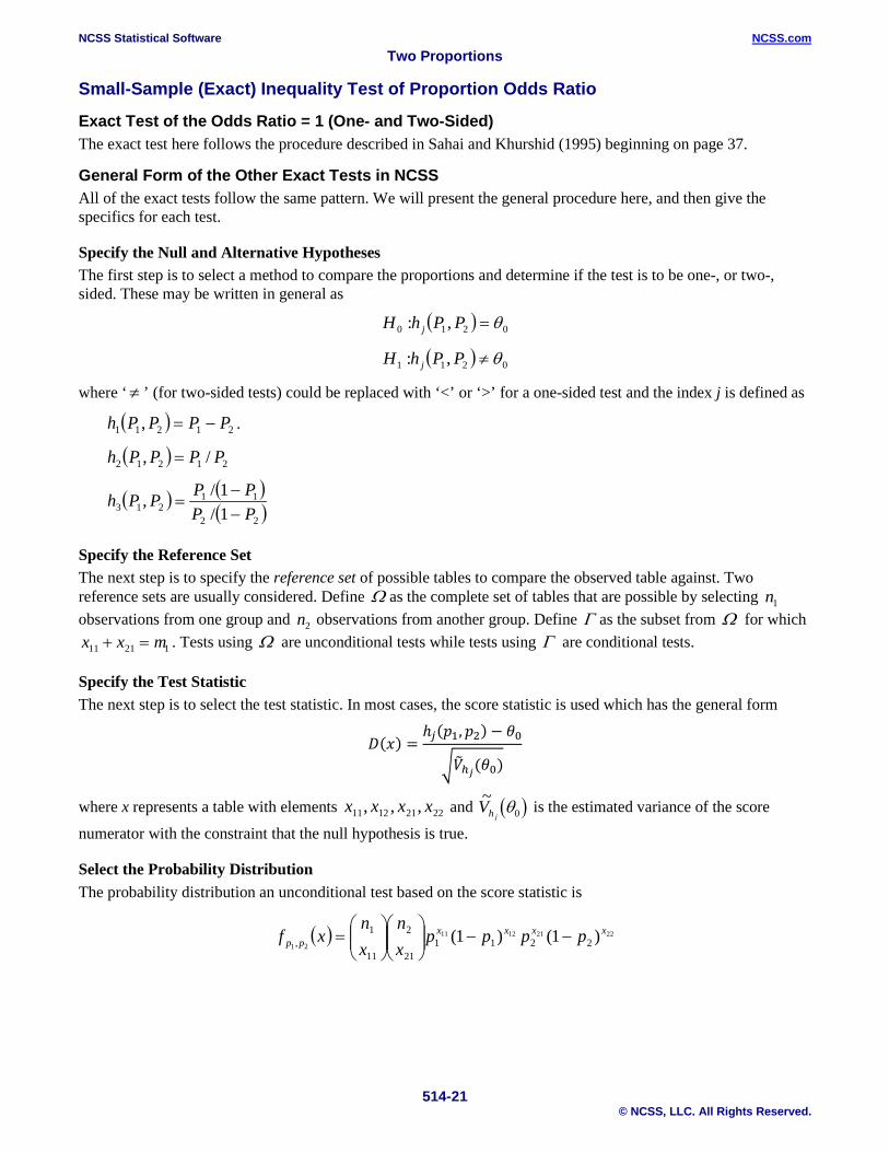
Small-Sample (Exact) Inequality Test of Proportion Odds Ratio
Exact Test of the Odds Ratio = 1 (One- and Two-Sided) The exact test here follows the procedure described in Sahai and Khurshid (1995) beginning on page 37.
General Form of the Other Exact Tests in NCSS All of the exact tests follow the same pattern. We will present the general procedure here, and then give the specifics for each test.
Specify the Null and Alternative Hypotheses The first step is to select a method to compare the proportions and determine if the test is to be one-, or two-, sided. These may be written in general as
( ) 0210 ,: θ=PPhH j
( ) 0211 ,: θ≠PPhH j
where ‘≠ ’ (for two-sided tests) could be replaced with ‘<’ or ‘>’ for a one-sided test and the index j is defined as
( ) 21211 , PPPPh −= .
( ) 21212 /, PPPPh =
( ) ( )( )22
11213 1/
1/,PPPPPPh
−−
=
Specify the Reference Set The next step is to specify the reference set of possible tables to compare the observed table against. Two reference sets are usually considered. Define Ω as the complete set of tables that are possible by selecting n1 observations from one group and n2 observations from another group. Define Γ as the subset from Ω for which x x m11 21 1+ = . Tests using Ω are unconditional tests while tests using Γ are conditional tests.
Specify the Test Statistic The next step is to select the test statistic. In most cases, the score statistic is used which has the general form
𝐷𝐷(𝑥𝑥) =ℎ𝑗𝑗(𝑝𝑝1,𝑝𝑝2) − 𝜃𝜃0
𝑉𝑉ℎ𝑗𝑗(𝜃𝜃0)
where x represents a table with elements 22211211 ,,, xxxx and ( )~Vh jθ0 is the estimated variance of the score
numerator with the constraint that the null hypothesis is true.
Select the Probability Distribution The probability distribution an unconditional test based on the score statistic is
( ) 22211211
21)1()1( 2211
21
2
11
1,
xxxxpp pppp
xn
xn
xf −−
=
NCSS Statistical Software NCSS.com Two Proportions
514-22 © NCSS, LLC. All Rights Reserved.
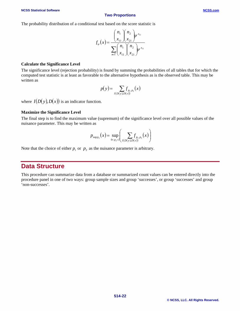
The probability distribution of a conditional test based on the score statistic is
( )∑
Γ∈
=
x
x
x
xn
xn
xn
xn
xf11
11
21
2
11
1
21
2
11
1
ψ
ψ
ψ
Calculate the Significance Level The significance level (rejection probability) is found by summing the probabilities of all tables that for which the computed test statistic is at least as favorable to the alternative hypothesis as is the observed table. This may be written as
( ) ( )( ) ( )( )∑=
xDyDIpp xfyp
,, 21
where ( ) ( )( )xDyDI , is an indicator function.
Maximize the Significance Level The final step is to find the maximum value (supremum) of the significance level over all possible values of the nuisance parameter. This may be written as
( ) ( )( ) ( )( )
= ∑
<< xDyDIpp
pp xfxp
,,
10sup 21
22
sup
Note that the choice of either p1 or p2 as the nuisance parameter is arbitrary.
Data Structure This procedure can summarize data from a database or summarized count values can be entered directly into the procedure panel in one of two ways: group sample sizes and group ‘successes’, or group ‘successes’ and group ‘non-successes’.
NCSS Statistical Software NCSS.com Two Proportions
514-23 © NCSS, LLC. All Rights Reserved.
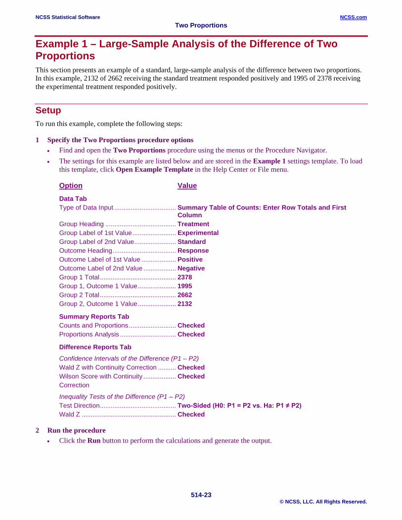
Example 1 – Large-Sample Analysis of the Difference of Two Proportions This section presents an example of a standard, large-sample analysis of the difference between two proportions. In this example, 2132 of 2662 receiving the standard treatment responded positively and 1995 of 2378 receiving the experimental treatment responded positively.
Setup To run this example, complete the following steps:
1 Specify the Two Proportions procedure options • Find and open the Two Proportions procedure using the menus or the Procedure Navigator. • The settings for this example are listed below and are stored in the Example 1 settings template. To load
this template, click Open Example Template in the Help Center or File menu.
Option Value Data Tab Type of Data Input .................................. Summary Table of Counts: Enter Row Totals and First
Column Group Heading ....................................... Treatment Group Label of 1st Value ........................ Experimental Group Label of 2nd Value ....................... Standard Outcome Heading ................................... Response Outcome Label of 1st Value ................... Positive Outcome Label of 2nd Value .................. Negative Group 1 Total .......................................... 2378 Group 1, Outcome 1 Value ..................... 1995 Group 2 Total .......................................... 2662 Group 2, Outcome 1 Value ..................... 2132
Summary Reports Tab Counts and Proportions .......................... Checked Proportions Analysis ............................... Checked
Difference Reports Tab Confidence Intervals of the Difference (P1 – P2) Wald Z with Continuity Correction .......... Checked Wilson Score with Continuity .................. Checked Correction
Inequality Tests of the Difference (P1 – P2) Test Direction .......................................... Two-Sided (H0: P1 = P2 vs. Ha: P1 ≠ P2) Wald Z .................................................... Checked
2 Run the procedure • Click the Run button to perform the calculations and generate the output.
NCSS Statistical Software NCSS.com Two Proportions
514-24 © NCSS, LLC. All Rights Reserved.
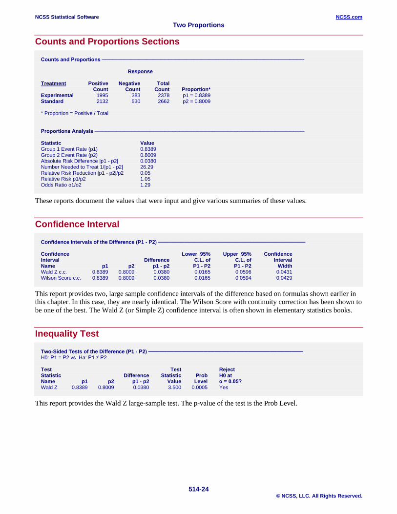
Counts and Proportions Sections
Counts and Proportions Response Treatment Positive Negative Total Count Count Count Proportion* Experimental 1995 383 2378 p1 = 0.8389 Standard 2132 530 2662 p2 = 0.8009 * Proportion = Positive / Total Proportions Analysis Statistic Value Group 1 Event Rate (p1) 0.8389 Group 2 Event Rate (p2) 0.8009 Absolute Risk Difference |p1 - p2| 0.0380 Number Needed to Treat 1/|p1 - p2| 26.29 Relative Risk Reduction |p1 - p2|/p2 0.05 Relative Risk p1/p2 1.05 Odds Ratio o1/o2 1.29
These reports document the values that were input and give various summaries of these values.
Confidence Interval
Confidence Intervals of the Difference (P1 - P2) Confidence Lower 95% Upper 95% Confidence Interval Difference C.L. of C.L. of Interval Name p1 p2 p1 - p2 P1 - P2 P1 - P2 Width Wald Z c.c. 0.8389 0.8009 0.0380 0.0165 0.0596 0.0431 Wilson Score c.c. 0.8389 0.8009 0.0380 0.0165 0.0594 0.0429
This report provides two, large sample confidence intervals of the difference based on formulas shown earlier in this chapter. In this case, they are nearly identical. The Wilson Score with continuity correction has been shown to be one of the best. The Wald Z (or Simple Z) confidence interval is often shown in elementary statistics books.
Inequality Test
Two-Sided Tests of the Difference (P1 - P2) H0: P1 = P2 vs. Ha: P1 ≠ P2 Test Test Reject Statistic Difference Statistic Prob H0 at Name p1 p2 p1 - p2 Value Level α = 0.05? Wald Z 0.8389 0.8009 0.0380 3.500 0.0005 Yes
This report provides the Wald Z large-sample test. The p-value of the test is the Prob Level.
NCSS Statistical Software NCSS.com Two Proportions
514-25 © NCSS, LLC. All Rights Reserved.
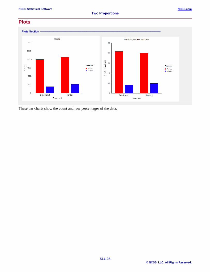
Plots
Plots Section
These bar charts show the count and row percentages of the data.