Chapter 6

Demand Estimation and Forecasting

6.1 MARKET RESEARCH APPROACHESA firm’s sales or demand can be estimated by market research approaches. These refer to consumer surveys, consumer clinics, and market experiments. Consumer surveys involve questioning a sample of consumers about how they would respond to particular changes in the price of the commodity and of related commodities, to changes in their incomes, and to changes in other determinants of demand. Consumer clinics are laboratory experiments in which participants are given a sum of money and asked to spend it in a simulated store to see how they react to changes in the commodity price, commodity packaging, displays, prices of competing commodities, and other factors affecting demand. In market experiments, the researcher changes the commodity price or other determinants of demand under experimental control (such as packaging and the amount and type of promotion) in a particular real-world store or stores and examines consumers’ responses to the changes.

Since many economic decisions (such as businesses’ plans to add to plant and equipment, and consumers intentions of purchasing houses, automobiles, washing machines, refrigerators, and so on) are made well in advance of actual expenditures, surveys and opinion polls on the buying intentions of businesses and consumers can be used to forecast a firm’s sales, or demand. These are often referred to as qualitative forecasts.

EXAMPLE 1. In 1962 University of Florida researchers conducted a market experiment in Grand Rapids, Michigan, to determine the price elasticity and cross-price elasticity of demand for three types of oranges: those from the Indian River district of Florida, those from the interior district of Florida, and those from California. Nine supermarkets participated in the experiment, which involved changing the prices of the three types of oranges each day for 31 consecutive days and recording the quantity sold of each variety. The researchers found that the price elasticity of demand for the three types of oranges was, respectively, –3.07, –3.01, and –2.76. They also found that while the cross-price elasticity of demand was larger than 1 between the two types of Florida oranges, it was less than 0.20 between each type of Florida orange and the California ones. Thus, consumers regarded the two types of Florida oranges as close substitutes, but they did not view the California oranges in that way. This information can be used to forecast the demand for each type of orange, resulting from changes in prices and in other determinants of demand.

EXAMPLE 2. Some of the best-known published surveys that can be used to forecast economic activity in general and in particular sectors of the economy are surveys of business executives’ plant and equipment expenditure plans (published in Business Week and in the Survey of Current Business), surveys of plans for inventory changes and sales expectations (conducted by the Department of Commerce, McGraw-Hill, the National Association of Purchasing Agents, and others), and surveys of consumer expenditure plans (conducted periodically by the Bureau of the Census and the Survey Research Center of the University of Michigan). For more specific forecasts of its own sales, a firm may rely on polls of its own executives and sales force or its own polls of consumer intentions.

6.2 TIME-SERIES ANALYSISOne of the most frequently used methods of forecasting a firm’s sales or demand is time-series analysis. Time-series data are data arranged chronologically by days, weeks, months, quarters, or years. Most economic time series exhibit a secular trend (long-run increases and decreases), cyclical fluctuations (the wavelike movement above and below the trend that appears every several years), seasonal variation (the fluctuations that regularly recur each year because of weather or social customs), and irregular or random influences arising from strikes, natural disasters, wars, or other unique events. While these components are shown separately for the time-series (sales) data in Fig. 6-1, they all operate at the same time in the real world.

The simplest form of time-series analysis is to forecast the past trend by fitting a straight line to the data (on the assumption that the past trend will continue in the future). The linear regression model will take the form of

St = S0 + bt (6-1)where St is the value of the time series in forecasting for period t, S0 is the estimated value of the time series (the constant of the regression) in the base period (i.e., at time period t = 0), b is the absolute amount of growth per period, and t is the time period in which the time series is to be forecasted (see Example 3).

Sometimes, an exponential trend (showing a constant percentage change rather than a constant amount of change in each period) fits the data better. The exponential trend model can be specified as

St = S0 (1 + g)t (6-2)where g is the constant percentage growth rate to be estimated. To estimate g, we transform equation (6-2) into natural logarithms and run the following regression:

ln St = ln S0 + t ln (1 + g) (6-2)Taking into consideration seasonal variation (when present) can significantly

improve the trend forecast and can be done by the ratio4o-trend method. To do so, we simply find the average ratio by which the actual value of the time series differs from the corresponding estimated trend value in each period and then multiply the

forecasted trend value by this ratio. (See Example 4.) An alternative is to use dummy variables.

Fig. 6-1

EXAMPLE 3. Fitting a trend line to the electricity sales data (consumption in millions of kilowatt-hours) running from the first quarter of 1985 (t = 1) to the last quarter of 1988 (t = 16) given in Table 6.1 we get

St = 11.90 + 0.394t R2 = 0.50(400)

Table 6.1

1986.41986.31986.21986.11985.41985.31985.21985.1Quarter

1613171214121511Quantity

1988.41988.31988.21988.11987.41987.31987.21987.1Quarter

1916201517151814Quantity

The regression results indicate that electricity sales in the last quarter of 1984 (i.e., S0) are estimated to be 11.90 million kwh and to increase at an average of 0.394 million kwh per quarter. The trend variable is statistically significant at better than the 1 percent level (from the t statistic below the estimated slope coefficient) and “explains” 50 percent of the variation in electricity consumption. Thus, based on the past trend, we can forecast electricity consumption (in million kwh) in the city to be

S17 = 11.90 + 0.394 (17) = 18.60 in the first quarter of 1989S18 = 11.90 + 0.394 (18) = 18.99 in the second quarter of 1989S19 = 11.90 + 0.394 (19) = 19.39 in the third quarter of 1989S20 = 11.90 + 0.394 (20) = 19.78 in the fourth quarter of 1989Similar results are obtained with an exponential trend (see Problem 6.6).

EXAMPLE 4. By incorporating the strong seasonal variation in the data in Table 6.1 (consumption in the second and fourth quarters of each year is consistently higher than in the first and third quarters) we can significantly improve the above forecast. To do this we first estimate, or forecast, electricity consumption in each quarter from 1985 to 1988 by substituting actual consumption into the above estimated equation. Then we find the ratio of actual to forecasted consumption in each quarter and calculate the average. This is shown in Table 6.2. Finally, we multiply the trend forecasts obtained in Example 3 by the average seasonal factors estimated in Table 6.2 (i.e., 0.887 for the first quarter, 1.165 for the second quarter, and so on) and get the following new forecasts based on both the linear trend and the

seasonal adjustment:S17 = 18.60(0.887) = 16.50 in the first quarter of 1989S18 = 18.99(1.165) = 22.12 in the second quarter of 1989 S19 = 19.39(0.097) = 17.59 in the third quarter of 1989S20 = 19.78(1.042) = 20.61 in the fourth quarter of 1989Note that with the inclusion of the seasonal adjustment, the forecasted values for electricity sales seem to closely replicate the past seasonal pattern (i.e., they are higher in the second and fourth quarters than in the first and third quarters). Similar results are obtained by using dummy variables. (See Problem 6.7.)

Table 6.2

Quarter Forecasted Actual Actual / Forecasted

1985.1 12.29 11.00 0.8951986.1 13.87 12.00 0.8651987.1 15.45 14.00 0.9061988.1 17.02 15.00 0.881

Average = 0.8871985.2 12.69 15.00 1.1821986.2 14.26 17.00 1.1921987.2 15.84 18.00 1.1361988.2 17.42 20.00 1.148

Average = 1.1651985.3 13.08 12.00 0.9171986.3 14.66 13.00 0.8871987.3 16.23 15.00 0.9241988.3 17.81 16.00 0.898

Average = 0.9071985.4 13.48 14.00 1.0391985.4 15.05 16.00 1.0631985.4 16.63 17.00 1.0221985.4 18.20 19.00 1.044

Average = 1.042

6.3 SMOOTHING TECHNIQUESSmoothing techniques can be used to forecast future values of a time series as some average of its past values when the series exhibits little trend or seasonal variation but a great deal of irregular or random variation. The simplest smoothing technique is the moving average. Here the forecasted value of a time series in a given period is equal to the average value of the series in a number of previous periods. For example, with a three-period moving average, the forecasted value of the time series for any period is given by the average value of the series in the previous three periods.

A better smoothing technique is exponential smoothing. Here the forecast for period t + 1 (i.e., Ft + 1) is a weighted average of the actual and forecasted values of the time series in period t. The value of the time series at period t (i.e., At) is assigned a weight (w) between 0 and 1 inclusive, and the forecast for period t (i.e., Ft) is then assigned the weight of 1 – w. The initial value of Ft is usually taken as the mean for the entire observed time series. The greater the value of w, the greater is the weight given to the value of the time series in period t as opposed to previous periods. The value of Ft + 1 is given by

Ft+1 = wAt + (1 – w ) Ft (6-4)To determine which moving average or weight in exponential smoothing leads to a better forecast, we calculate the root mean square error (RMSE) of each forecast and utilize the forecast with the lowest RMSE. The formula for RMSE is

(6-5)

where stands for “the sum of,” “i is the index variable,” At is the actual value of the time series in period t, Ft is the forecasted value, and n is the number of time periods or observations. The forecast difference (i.e., A – F) is squared in order to penalize larger errors proportionately more than smaller ones.

EXAMPLE 5. Table 6.3 shows the calculation of a three-quarter and a five-quarter moving average for a firm’s market share during eight quarters [columns (1) and (2)]. The forecast for the fourth quarter in column (3) is equal to the average of the values for the first three quarters in column (2). For the ninth quarter, the forecast is 19.67 with a three-quarter moving average and 20.6 with a five-quarter moving average.

The RMSEs are, respectively:

Since the three-quarter moving average forecast has the lower RMSE, we prefer it.

Table 6.3

Quarter

Firm’s Actual Market Share

(A)

Three-Quarter Moving Average

Forecast (F) A – F (A – F)2

Five-Quarter Moving Average

Forecast (F) A – F (A – F)2

( 1 ) ( 2 ) ( 3 ) ( 4 ) ( 5 ) ( 6 ) ( 7 ) ( 8 )

1 20 –– –– –– –– –– ––2 22 –– –– –– –– –– ––3 23 –– –– –– –– –– ––4 24 21.67 2.33 5.4289 –– –– ––5 20 23.00 –3.00 9.0000 –– –– ––6 23 22.33 0.67 0.4489 21.8 1.2 1.447 19 22.33 –3.33 11.0889 22.4 –3.4 11.568 17 20.67 –3.67 13.4689 21.8 –4.8 23.049 –– 19.67 –– –– 20.6 –– ––

Total –– –– –– 39.4356 –– –– 36.04

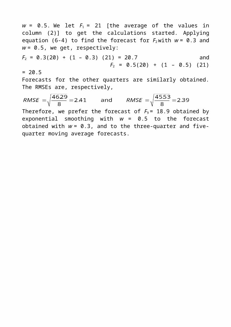
EXAMPLE 6. Table 6.4 shows the calculations used to obtain forecasts for the firm’s market share data in Table 6.3 by exponential smoothing with w = 0.3 andw = 0.5. We let F1 = 21 [the average of the values in column (2)] to get the calculations started. Applying equation (6-4) to find the forecast for F2 with w = 0.3 and w = 0.5, we get, respectively:F2 = 0.3(20) + (1 – 0.3) (21) = 20.7 and F2 = 0.5(20) + (1 – 0.5) (21) = 20.5Forecasts for the other quarters are similarly obtained. The RMSEs are, respectively,

Therefore, we prefer the forecast of F9 = 18.9 obtained by exponential smoothing with w = 0.5 to the forecast obtained with w = 0.3, and to the three-quarter and five-quarter moving average forecasts.

Table 6.4

QuarterFirm’s Actual

Market Share (A)Forecast (F)

with w = 0.3 A – F (A – F)2

Forecast (F)with w = 0.3 A – F (A – F)2

( 1 ) ( 2 ) ( 3 ) ( 4 ) ( 5 ) ( 6 ) ( 7 ) ( 8 )

1 20 21.0 –1.0 1.00 21.0 –1.0 1.002 22 20.7 1.3 1.69 20.5 1.5 2.253 23 21.1 1.9 3.61 21.3 1.7 2.894 24 21.7 2.3 5.29 22.2 1.8 3.245 20 22.4 –2.4 5.76 23.1 –3.1 9.616 23 21.7 1.3 1.69 21.6 1.4 1.967 19 22.1 –3.1 9.61 22.3 –3.3 10.898 17 21.2 –4.2 17.64 20.7 –3.7 13.699 –– 19.9 –– –– 18.9 –– ––

Total –– –– –– 46.29 –– –– 45.53

6.4 BAROMETRIC METHODSBarometric forecasting relies on changes in leading indicators (time series that anticipate or lead changes in general economic activity) to forecast turning points (peaks and troughs) in business cycles. While our interest is primarily in leading indicators, some time series move in step, or coincide, with movements in general economic activity and are therefore called coincident indicators. Still others follow, or lag behind, movements in economic activity and are called lagging indicators (see Problem 6.11). Table 6.5 presents a list of the 12 best leading indicators (out of a much longer list available), together with their mean lead ( – ) time (in months) with respect to the actual cyclical peak or trough.

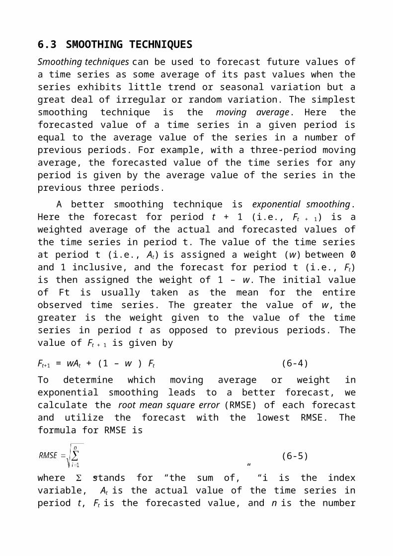
Table 6.5 Short List of 12 Leading Indicators

Indicators Lead in Months

Average work week of production workers, manufacturing –7.3Layoff rate, manufacturing –8.6New orders, consumer goods and materials, 1972 dollars –6.7Vendor performance, companies receiving slower deliveries –7.3Index of net business formation –7.4Contracts and orders, plant and equipment, 1972 dollars –5.5New building permits, private housing units –10.9Change in inventories on hand and on order, 1972 dollars –5.6Change in sensitive materials prices –8.8Stock prices, 500 common stocks –7.0Change in total liquid assets-8.5 –8.5Money supply (M2), 1972 dollars –11.8

Composite index of the 12 leading indicators –8.2

Source: U. S. Department of Commerce, Bureau of Economic Analysis, Handbook of Cyclical Indicators (Washington, D. C.: U. S. Government Printing office, May 1977), pp. 174-191.

Table 6.5 also gives the composite index, a weighted average of the 12 leading indicators, with larger weights assigned to those indicators that do a better job of forecasting. The composite index smooths out random variations and provides more reliable forecasts and fewer wrong signals than individual indicators. Another method of overcoming the difficulty arising when some of the 12 leading indicators move up and some move down is the diffusion index. This gives the percentage of the 12 leading indicators that are moving up. All these indicators are published monthly in Business Conditions Digest by the U.S. Department of Commerce. Three or four successive one-month declines in the composite index and a diffusion index of less than 50 percent are usually a prelude to a recession, (i.e., a slowing down) of economic activity.

Fig. 6-2

EXAMPLE 7. The top panel of Fig. 6-2 shows that the composite index of 12 leading indicators turned down prior to (i.e., led) the recessions of 1969-1970, 1973-1975, 1980, and 1981-1982 (the shaded regions in the figure). The bottom panel shows that the diffusion index for the leading indicators was generally below 50 percent in the months preceding recessions.

6.5 ECONOMETRIC METHODSThe most common method of estimating and forecasting firm’s sales or demand

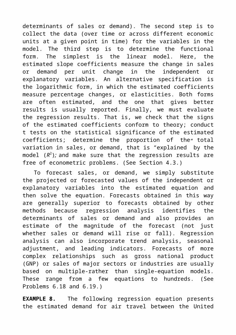
is regression analysis. The first step is to specify the model, (i.e., to identify the determinants of sales or demand). The second step is to collect the data (over time or across different economic units at a given point in time) for the variables in the model. The third step is to determine the functional form. The simplest is the linear model. Here, the estimated slope coefficients measure the change in sales or demand per unit change in the independent or explanatory variables. An alternative specification is the logarithmic form, in which the estimated coefficients measure percentage changes, or elasticities. Both forms are often estimated, and the one that

gives better results is usually reported. Finally, we must evaluate the regression results. That is, we check that the signs of the estimated coefficients conform to theory; conduct t tests on the statistical significance of the estimated coefficients; determine the proportion of the total variation in sales, or demand, that is “explained” by the model (R2); and make sure that the regression results are free of econometric problems. (See Section 4.3.)

To forecast sales, or demand, we simply substitute the projected or forecasted values of the independent or explanatory variables into the estimated equation and then solve the equation. Forecasts obtained in this way are generally superior to forecasts obtained by other methods because regression analysis identifies the determinants of sales or demand and also provides an estimate of the magnitude of the forecast (not just whether sales or demand will rise or fall). Regression analysis can also incorporate trend analysis, seasonal adjustment, and leading indicators. Forecasts of more complex relationships such as gross national product (GNP) or sales of major sectors or industries are usually based on multiple-rather than single-equation models. These range from a few equations to hundreds. (See Problems 6.18 and 6.19.)

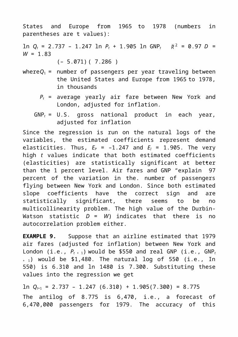
EXAMPLE 8. The following regression equation presents the estimated demand for air travel between the United States and Europe from 1965 to 1978 (numbers in parentheses are t values):

ln Qt = 2.737 – 1.247 ln Pt + 1.905 ln GNPt = 0.97 D = W = 1.83(– 5.071) ( 7.286 )

where Q1 = number of passengers per year traveling between the United States and Europe from 1965 to 1978, in thousands

Pt = average yearly air fare between New York and London, adjusted for inflation.

GNPt = U.S. gross national product in each year, adjusted for inflationSince the regression is run on the natural logs of the variables, the estimated coefficients represent demand elasticities. Thus, EP = –1.247 and EI = 1.905. The very high t values indicate that both estimated coefficients (elasticities) are statistically significant at better than the 1 percent level. Air fares and GNP “explain” 97 percent of the variation in the. number of passengers flying between New York and London. Since both estimated slope coefficients have the correct sign and are statistically significant, there seems to be no multicollinearity problem. The high value of the Durbin-Watson statistic D = W) indicates that there is no autocorrelation problem either.

EXAMPLE 9. Suppose that an airline estimated that 1979 air fares (adjusted for inflation) between New York and London (i.e., Pt + 1) would be $550 and real GNP (i.e., GNPt + 1) would be $1,480. The natural log of 550 (i.e., In 550) is 6.310 and ln 1480 is 7.300. Substituting these values into the regression we get

ln Qt+1 = 2.737 – 1.247 (6.310) + 1.905(7.300) = 8.775The antilog of 8.775 is 6,470, i.e., a forecast of 6,470,000 passengers for 1979. The accuracy of this forecast depends on the accuracy of the estimated demand coefficients and of the estimated or forecasted values of the independent or explanatory variables in the demand equation.

Glossary

Barometric forecasting The method of forecasting turning points in business cycles by the use of leading economic indicators.

Coincident indicators Time series that move in step, or coincide, with movements in the level of general economic activity.

Composite index An index formed by a weighted average of the individual indicators.

Consumer clinics Laboratory experiments in which the participants are given a sum of money and asked to spend it in a simulated store to see how they react to changes in the commodity price and other determinants of demand.

Consumer surveys The questioning of a sample of consumers about how they would respond to particular changes in the price and other determinants of the demand for a commodity.

Cyclical fluctuations The major expansions and contractions in most economic time series that recur every number of years.

Diffusion index An index that measures the percentage of the 12 leading indicators that are moving upward.

Exponential smoothing A smoothing technique in which the forecast for a period is a weighted average of the actual and forecasted values of the time series in the previous period.

Irregular or random influences The unpredictable variations in a data series resulting from wars, natural disasters, strikes, or other unforeseen events.

Lagging indicators Time series that follow, or lag behind, movements in the level of general economic activity.

Leading economic indicators Time series that tend to precede, or lead, changes in the level of general economic activity.

Market experiments Attempts by the firm to estimate the demand for a commodity by changing price and other determinants of the demand for the commodity in the actual marketplace (i.e., in some stores).

Moving average The smoothing technique in which the forecasted value of a time series in a given period is equal to the average value of the time series in a number of previous periods.

Qualitative forecasts The estimation of the future value of a variable (such as the firm’s sales) based on surveys and opinion polls of businesses’ and consumers’ buying intentions.

Root mean square error (RMSE) The measure of the weighted average error of a forecast.

Seasonal variation The regularly recurring fluctuations in economic activity that occur during each year because of weather and social customs.

Secular trend The long-run increase or decrease in a data series.

Smoothing techniques A method of naive forecasting in which future values of a time series are forecasted on the basis of some average of its past values only.

Time-series analysis The technique of forecasting future values of a time series by examining past observations of the time-series data only.

Time-series data The values of a variable arranged chronologically by days, weeks, months, quarters, or years.

Review Questions

1. Which of the following is not a marketing research approach to demand estimation?(a) Consumer clinics(b) Regression analysis(c) Market experiments(d) Consumer surveys

Ans. (b) See Section 6.1.

2. Consumer surveys refer to(a) laboratory experiments in which the participants are given a sum of money

and asked to spend it in a simulated store to see how they react to changes in the factors affecting demand.

(b) changes in the commodity price or other determinants of demand under the control of the firm, including control in a particular store or stores and examination of consumers’ responses to the changes.

(c) questioning a sample of consumers about how they would respond to particular changes in the price of the commodity and of related commodities, to changes in their incomes, and to changes in other determinants of demand.

(d) any of the above.

Ans. (c) See Section 6.1.

3. Which of the following statements is false?(a) Qualitative forecasting is based on surveys and opinion polls of the buying

intentions of businesses and consumers.(b) Surveys of plant and equipment expenditure plans of business executives

are published in Business Week and in the Survey of Current Business.(c) Firms sometimes forecast their sales by polling consumers directly.(d) None of the above.

Ans. (d) See Section 6.1 and Example 2.

4. Yearly sales data exhibit no(a) trend.(b) cyclical variation.(c) seasonal variation.(d) irregular variation.

Ans. (c) See Section 6.2.

5. Time-series analysis(a) seeks to forecast a time series based on its past values only.(b) seeks to explain the underlying causes of the variation in the data.(c) can explain the irregular variation in the data.(d) all of the above.

Ans. (a) See Section 6.2.

6. Which of the following statements is true with regard to time-series analysis?(a) The ratio-to-trend method is used to adjust the trend forecast for the

seasonal variation in the data.(b) Sometimes an exponential trend fits time-series data better than a linear

trend.(c) The seasonal variation in the data can he taken into consideration by using

dummy variables.(d) All of the above.

Ans. (d) See Section 6.2.

7. Smoothing techniques are useful methods of forecasting.(a) the trend in a time series.(b) cyclical fluctuations.(c) the seasonal variation in a time series.(d) irregular or random influences in the data.

Ans. (d) See Section 6.3.

8. Which of the following statements is false with regard to smoothing techniques?(a) The greater the number of periods used to calculate a moving average, the

smaller will be the degree of smoothing in the time series.(b) Exponential smoothing usually gives better forecasts than moving

averages.

(c) The reliability of forecasts can be compared using the root mean square error.

(d) None of the above.

Ans. (a) See Section 6.3.

9. Which of the following statements is false with regard to barometric forecasting?(a) It relies on changes in leading indicators to forecast changes in the level of

economic activity, just as changes in the mercury in a barometer are used to forecast changes in weather conditions.

(b) Turning points in business cycles are usually forecasted with the composite and diffusion indexes of leading indicators.

(c) A fall in the composite and diffusion indexes in a given month is used to predict a recession.

(d) Barometric forecasting gives no indication of the magnitude of the forecasted change in the level of economic activity.

Ans. (c) See Section 6.4.

10. In the process of estimating the demand for a commodity by regression analysis, the researcher needs to(a) determine the variables and equational form of the model.(b) collect the data on the variables of the model.(c) evaluate the regression results.(d) do all of the above.

Ans. (d) See Section 6.5.

11. Which of the following statements is false with regard to the estimation of demand by regression analysis?(a) Specifying the model means identifying the variables in the model.(b) Time-series data are required.(c) Either a linear or a log demand equation can be estimated.(d) Evaluating the regression results involves determining, among other things,

whether the estimated coefficients have the signs postulated by theory.

Ans. (b) See Section 6.5.

12. Which of the following statements is false with regard to forecasting with econometric models?(a) It is accomplished by substituting into the estimated regression equation the

estimated or forecasted values of the independent or explanatory variables and solving.

(b) It usually provides better forecasts than other forecasting methods.(c) It cannot be combined with other forecasting methods.(d) It provides not only the direction of change in the variable to be forecasted,

but also an estimate of the magnitude of the change.

Ans. (c) See Section 6.5.

Solved Problems

MARKET RESEARCH APPROACHES TO DEMAND ESTIMATION

6.1 (a) What is meant by consumer surveys? How can they be used to estimate demand? (b) What are their advantages? (c) What are their disadvantages?(a) Consumer surveys involve questioning a sample of consumers about how

they would respond to particular changes in the following: the price of the commodity and of related commodities, changes in their incomes, changes in advertising, credit incentives, and other determinants of demand. These surveys can be conducted by simply stopping people at a shopping center or by developing sophisticated questionnaires administered to a carefully constructed representative sample of consumers by trained interviewers.

(b) The major advantages of estimating demand using consumer surveys are: (1) Surveys may be the only way to obtain information about consumers’ possible responses to the introduction of a new commodity, changes in consumers’ tastes and preferences, and consumers’ expectations about future prices and business conditions. Survey results that show consumers are unaware of price differences between the firm’s product and competing products may be a good indication that demand for the firm’s product is price inelastic. (2) Consumer surveys can be made as simple or as elaborate as desired. (3) The researcher can ask specific questions pertaining to the demand for the product.

(c) The major disadvantages of consumer surveys are: (1) Consumers may be unable or unwilling to provide reliable answers. For example, do you know by how much your monthly beer consumption would change if the price of beer rose by 10 cents per bottle? if the price of sodas fell by 5 cents? if your income rose by 20 percent? or if a beer producer doubled its advertising expenditures? Even if you tried to answer these questions as accurately as possible, your reaction might be entirely different if you were actually faced with any of the above situations. Sometimes consumers provide a response that they deem more socially acceptable rather than disclose their true preferences. (2) Depending on the size of the sample and the elaborateness of the analysis, consumer surveys can also be rather expensive.

6.2 (a) What is meant by consumer clinics? How can they be used to estimate demand? (b) What is their advantage? (c) What are their disadvantages?(a) Consumer clinics are laboratory experiments in which the participants are

given a sum of money and asked to spend it in a simulated store to see how they react to changes in the commodity price, product packaging,

displays, prices of competing products, and other factors affecting demand. Participants in the experiment can be selected so as to closely represent the socioeconomic characteristics of the market of interest.

(b) By simulating how consumers behave in an actual market situation rather than simply asking them how they think they would behave, consumer clinics attempt to overcome the major disadvantage of consumer surveys.

(c) The main disadvantages of consumer clinics are: (1) Participants know that they are in an artificial situation and that they are being observed, so they are not likely to act normally. For example, suspecting that the researchers might be interested in their reaction to price changes, participants are likely to show more sensitivity to price changes than in their everyday shopping. (2) The sample of participants must necessarily be small because of the high cost of running the experiment. However, inferring market behavior from the results of an experiment based on a very small sample can be dangerous.

6.3 (a) What is meant by market experiments? Row can they be used to estimate demand? (b) What are their advantages? (c) What are their disadvantages?(a) Unlike consumer clinics, which are conducted under strict laboratory

conditions, market experiments are conducted in the actual market place. There are many different ways of performing market experiments. One method is to select several markets with similar socioeconomic characteristics. The researcher then changes the commodity price in some markets or stores, the packaging in other markets or stores, and the amount and type of promotion in still other markets or stores, and records the responses (purchases) of consumers in the different markets. Alternatively, the researcher could change, one at a time, each of the determinants of demand under its control in a particular market over a period of time. and record consumers responses.

(b) The major advantages of estimating demand by market experiments are: (1) Consumers are in a real market situation and do not know that they are being observed. (2) The experiments can be conducted on a large scale, with some controls, so as to ensure the validity of the results.

(c) The major disadvantages of using market experiments to estimate demand are: (1) In order to keep costs down, the experiment is likely to be conducted on too limited a scale and over too short a period of time, so that inferences about the entire market, over a more extended period of time, will be questionable. (2) Extraneous occurrences, such as a strike or unusually bad weather, may seriously bias the results of a market experiment. (3) Competitors could try to sabotage the experiment by also changing prices and other determinants of demand under their control, or they could monitor the experiment and gain very useful information that the firm would prefer not to disclose. (4) The firm may permanently lose

customers in the process of raising prices in the market where it is experimenting with a high price.

6.4 (a) What is meant by forecasting? Why is it so important in the management of business firms and other enterprises? (b) What are qualitative forecasts? What is their rationale and usefulness? (c) What are the most important surveys of future economic activities? (d) Why and how do firms conduct opinion polls of future economic activities?(a) Forecasting is the process of estimating a variable, such as the sales of the

firm, at some future date. Forecasting is important to business firms, government, and not-for-profit organizations as a method of reducing the risk and uncertainty inherent in most managerial decisions.

(b) Qualitative forecasts estimate variables at some future date using the results of surveys and opinion polls of business and consumer spending intentions. The rationale is that many economic decisions are made well in advance of actual expenditures. For example, businesses usually plan to add to plant and equipment long before expenditures are actually incurred. Also, surveys and opinion polls are often used to make short-term forecasts when quantitative data are not available. Polls can also be very useful in supplementing quantitative forecasts, anticipating changes in consumer tastes or business expectations about future economic conditions, and forecasting the demand for a new product.

(c) Some of the best-known surveys are the ones conducted periodically on business executives’ plant and equipment expenditure plans, plans for inventory changes, sales expectations, and on consumers’ expenditure plans. In general, the record of these surveys has been rather good in forecasting actual expenditures.

(d) While the results of published surveys of expenditure plans of businesses, consumers, and governments are useful, the firm usually needs specific forecasts of its own sales. The firm can base its sales forecasts on polls of its top executives or outside experts, polls of its sales force in the field, or polls of a sample of consumers on their intentions to purchase some particular durable good, such as a house, an automobile, or a major appliance.

TIME-SERIES ANALYSIS

6.5 Draw a figure showing the linear trend and trend forecasts obtained in Example 3. On the same figure show also the trend forecasts adjusted for the seasonal variation obtained in Example 4.

See Fig. 6-3. The forecasts based only on the extension of the linear trend are shown by the dots on the dashed portion of the estimated trend line

extended into 1989. On the other hand, the forecasts obtained by adjusting the trend forecasts to take into consideration the seasonal variation in the data are shown by the encircled points in the figure. The latter seem to closely replicate the past seasonal pattern in the data.

Fig. 6-3

6.6 (a) Fit an exponential trend to the data of Table 6.1. (b) Use the results to forecast electricity sales during each quarter of 1989. (c) Compare these forecasts with those obtained by using the estimated linear trend in Example 3(a) To run regression equation (6-3) we must first transform the data on

electricity sales given in Table 6.1 into their natural logarithms. For example, the in of 11 (the value in Table 6.1 for the first quarter of 1985) is 2.40 (obtained by simply entering the value of 11 into any full-function pocket calculator and pressing the “In” key). Running regression (6-3), we get

ln St = ln So + t ln (1 + g)= 2.4765 + 0.026t R2 = 0.50

(4.06)The fit is very similar to that found in Example 3. Since the estimated parameters are now based on the logarithms of the data, however, we

must convert them into their antilogs in order to be able to interpret them in units of the original data. The antilog of In S0 = 2.4765 is S0 = 11.90 (obtained by simply entering the value of 2.4765 into any full-function pocket calculator and pressing the “ex ” key) and the antilog of In (1 + g) = 0.026 gives (1 + g) = 1.026. Substituting these values back into the above estimated regression equation, we have

St = 11.90(1.026)t

where S0 = 11.90 million kilowatt-hours is the estimated sales of electricity in the fourth quarter of 1984 (i.e., at t = 0) and the estimated growth rate is 1.026, or 2.6 percent per quarter.

(b) To forecast sales in any future quarter, we substitute the value of t for that quarter into the last equation above and solve for St . Thus,

S17 = 11.90 (1.026 )17 = 18.41 in the first quarter of 1989 S18 = 11.90 (1.026 )18 = 18.89 in the second quarter of 1989S19 = 11.90 (1.026 )19 = 19.38 in the third quarter of 1989S20 = 11.90 (1.026 )20 = 19.88 in the forth quarter of 1989

(c) The forecasts obtained in part (b) are very similar to those obtained by using the fitted linear trend. Note that the forecasts obtained by the two methods differ by increasing amounts as the time series is forecasted further into the future. This is usually the case. In the real world, both the linear and the exponential trends are usually fitted to the data, and the one that gives the better results is then used in forecasting.

6.7 Using the data on electricity consumption given in Table 6.1 in Example 3, (a) run a linear regression with the trend variable and seasonal dummies (see Problem 4.7) as independent or explanatory variables. (b) Use the estimated regression equation to forecast electricity sales for each quarter of 1989 and (c) compare these forecasts with those obtained in Example 4.(a) We take the last quarter as the base-period quarter and define dummy

variable D1 by a time series with 1 in the first quarter of each year and 0 in the other quarters, D2 by a time series with 1 in the second quarter of each year and 0 in the other quarters, and D3 by 1 in the third quarter of each year and 0 in the other quarters. We then obtain the following results by running a regression of electricity sales on the seasonal dummy variables and the linear time trend:St = 12.75 – 2.375D1t + 1.750D2t – 2.125D3t + 0.375t R2 = 0.99

(–10.38) (8.11) (–9.94) (22.25)Note that the estimated coefficients for the dummy variables and the trend variable are all statistically significant at better than the 1 percent level and that the regression “explains” 99 percent of the variation in electricity sales as compared with only 50 percent for the regression in Example 3.

(b) Utilizing the regression results obtained in part (a), we can forecast electricity sales for each quarter of 1989 to be:

S17 = 12.75 – 2.375 + 0.375(17) = 16.75 in the first quarter of 1989S18 = 12.75 + 1.750 + 0.375(18) = 21.25 in the second quarter of 1989S19 = 12.75 – 2.125 + 0.375(19) = 17.75 in the third quarter of 1989S20 = 12.75 + 0.375(20) = 20.25 in the forth quarter of 1989

(c) These forecasted values are very similar to those obtained by the ratio-to-trend method in Example 4. Thus, in this case the two methods are good alternatives for taking into consideration the seasonal variation in the forecasts. It is important to remember, however, that these forecasts are based on the assumption that the past trend and seasonal patterns in the data will persist during 1989. If the pattern suddenly changes in a drastic manner, the forecasts are likely to be far off the mark. This is more likely the further into the future we attempt to forecast.

SMOOTHING TECHNIQUES

6.8 Using the index (with 1971 = 100) of new housing starts in a large metropolitan area in the table below, forecast the index for 1986, using a three-year and a five-year moving average. In which of the forecasts would we have more confidence?

Year 1976 1977 1978 1979 1980 1981 1982 1983 1984 1985

Index 132 127 120 75 87 125 92 134 128 140

The calculations needed to answer this problem are shown in Table 6.6. The RMSEs for the three-year and the five-year moving average forecasts are, respectively:

Since RMSE for the five-year moving average forecast is smaller than for the three-year moving average forecast, we prefer the former forecast of 123.8 to the latter forecast of 134.0 for 1986.

6.9 Using the data in column (2) of Table 6.6 and the method of exponential smoothing, with w = 0.3 and w = 0.5, forecast (to one decimal place) the index of new housing starts for the year 1986. Which of the two forecasts is better?

Table 6.6

Quarter

Index of New Housing

Starts (A)

Three-Quarter Moving Average

Forecast (F) A – F (A – F)2

Five-Quarter Moving Average

Forecast (F) A – F (A – F)2

( 1 ) ( 2 ) ( 3 ) ( 4 ) ( 5 ) ( 6 ) ( 7 ) ( 8 )

1976 132 –– –– –– –– –– ––

1977 127 –– –– –– –– –– ––

1978 120 –– –– –– –– –– ––

1979 75 126.3 –51.3 2,631.69 –– –– ––

1980 87 107.3 –20.3 412.09 –– –– ––

1981 125 94.0 31.0 961.00 108.2 16.8 282.24

1982 92 95.7 –3.3 13.69 106.8 –14.8 219.04

1983 134 101.3 32.7 1,069.29 99.8 34.2 1,169.64

1984 128 117.0 11.0 121.00 102.6 25.4 645.16

1985 140 118.0 22.0 484.00 113.2 26.8 718.24

1986 –– 134.0 –– –– 123.8 –– ––

Total –– –– –– 5,692.76 –– –– 3,034.32

The calculations needed to answer this problem are shown in Table 6.7. The forecasts in columns (3) and (6) of the table are obtained by applying equation (6-4) with w = 0.3 and w = 0.5, respectively. We let F1976 = 116.0 [the average value of column (2)] to get the calculations started in both cases. The RMSEs for the forecasts obtained with w = 0.3 and w = 0.5 are, respectively:

Since the RMSE of the forecast of F1986 = 124.1, obtained by exponential smoothing with w = 0.3, is smaller than the RMSE for the forecast of F1986 = 131.4 obtained with w = 0.5, we prefer the former to the latter forecast. The forecast obtained by exponential smoothing with w = 0.3 is also superior to the three- and five-year moving average forecasts obtained in Problem 6.8.

Table 6.7

Quarter (A)F withw = 0.3 A – F (A – F)2

F withw = 0.5 A – F (A – F)2

( 1 ) ( 2 ) ( 3 ) ( 4 ) ( 5 ) ( 6 ) ( 7 ) ( 8 )

1976 132 116.0 16.0 256.00 116.0 16.0 256.00

1977 127 120.8 6.2 38.44 124.0 3.0 9.00

1978 120 122.7 –2.7 7.29 125.5 –5.5 30.25

1979 75 121.9 –56.9 2,199.61 122.8 –47.8 2,284.84

1980 87 107.8 –20.8 432.64 98.9 –11.9 141.61

1981 125 101.6 23.4 547.56 93.0 32.0 1,024.00

1982 92 108.6 –16.6 275.56 109.0 –17.0 289.00

1983 134 103.6 30.4 924.16 100.5 33.5 1,122.25

1984 128 112.7 15.3 234.09 117.3 10.7 144.49

1985 140 117.3 22.7 515.29 122.7 17.3 299.29

1986 –– 124.1 –– –– 131.4 –– ––

Total –– –– –– 5,430.64 –– –– 5,570.73

BAROMETRIC METHODS

6.10 Draw a figure showing the positions of the leading, coincident, and lagging indicators relative to the peak and trough of a business cycle.

See Fig. 6-4. The figure shows that leading indicators precede business cycle peaks and troughs, coincident indicators move in step with business cycles, while lagging indicators follow, or lag behind, turning points in business cycles.

Fig. 6-4

6.11 Using the publication given at the bottom of Table 6.5 in Example 6, identify the short list of coincident and lagging indicators, and indicate their lead ( – ) or lag ( + ) time. Also indicate the lead or lag time for the composite indexes of the short list of coincident and lagging indicators.

See Table 6.8. For the sake of comprehensiveness and comparison, Table 6.8 also includes the short list of leading indicators given in Table 6.5. From Table 6.8, it can be seen that the composite index of coincident indicators in fact leads the peaks and troughs in business cycles by about 1.2 months. The composite index of the lagging indicators lags behind the business cycle peaks and troughs by an average of 4.8 months.

Table 6.8 Short List of Leading, Coincident, and Lagging Indicators

Indicators Lead ( – ) or Lag ( + )

Leading indicators (12 series)Average work week of production workers, manufacturing –7.3Layoff rate, manufacturing –8.6New orders, consumer goods and materials, 1972 dollars –6.7Vendor performance, companies receiving slower deliveries –7.3Index of net business formation –7.4Contracts and orders, plant and equipment, 1972 dollars –5.5New building permits, private housing units –10.9Change in inventories on hand and on order, 1972 dollars –5.6Change in sensitive materials prices –8.8Stock prices, 500 common stocks –7.0Change in total liquid assets –8.5Money supply (M2), 1972 dollars –11.8

Roughly coincident indicators (4 series)Employees on nonagricultural payrolls –0.3Personal income, 1972 dollars –0.6Industrial production –1.6Manufacturing and trade sales, 1972 dollars –2.3

Lagging indicators (6 series)Average duration of unemployment +4.9Manufacturing and trade inventories, 1972 dollars +4.0Labor cost per unit of output, manufacturing +9.0Average prime rate charged by banks +7.1Commercial and industrial loans outstanding +3.9Ratio, consumer installment debt to personal income +5.6

Composite indexesTwelve leading indicators –8.2Four roughly coincident indicators –1.2Six lagging indicators +4.8

Source: U. S. Department of Commerce, Bureau of Economic Analysis, Handbook of Cyclical Indicators (Washington, D. C.: U. S. Government Printing office, May 1977), pp. 174-191

6.12 Table 6.9 gives the monthly composite and diffusion indexes for the 12 leading indicators for 1986. (a) Did the changes in the indexes for the first part of 1986 correctly anticipate or forecast the moderate growth that in retrospect we know occurred in the latter part of the year? (b) Based on the changes in the indexes in the second half of 1986, what changes in the level of economic activity can you forecast for 1987?

Table 6.9 Monthly Composite and Diffusion Index forthe 12 Leading Indicators during 1986

Month Composite Index Diffusion Index

January 173.4 62.5February 174.9 50.0March 175.9 62.5April 178.2 75.0May 178.1 50.0June 177.7 54.2July 179.3 62.5August 179.1 41.7September 179.4 54.2October 180.6 41.7November 182.2 75.0December 186.1 77.3

Source: U. S. Department of Commerce, Bureau of Economic Analysis, Business Conditions Digest, (Washington, D. C.: U. S. Government Printing office, January 1987), pp. 60-74

(a) Since the composite index increased modestly from January to April 1986 and declined very slightly during May and June, and at the same time the diffusion index was 50 percent or more but never exceeded 75 percent, we would have forecasted moderate growth for the latter part of the year. This is in fact what occurred.

(b) With the continued modest rise (except in August 1986) in the composite index and with a diffusion index above 50 percent (except in August and October) but never above 77.3 percent, we can forecast moderate growth for the first part of 1987 as well. To be pointed out, however, is that barometric forecasting is only 80 to 90 percent accurate in forecasting turning points. It also does not provide any indication of the magnitude of the forecasted change in the level of economic activity. Thus, barometric forecasting is most useful when used in conjunction with econometric forecasting, which does give an estimate of the magnitude of the forecasted changes.

ECONOMETRIC METHODS

6.13 By using regression analysis, Houthakker and Taylor estimated the following demand equation for shoes in the United States over the period from 1929 to 1961:

Qt = 19.575 – 0.0923Pt + 0.0289Xt – 99.568Ct – 4.06Dt

(–1.7682) (9.3125) (9.8964) (3.50)

where Qt = per capita personal consumption expenditures on shoes and other footwear during year t, in 1954 prices

Pt = relative price of shoes in year t, in 1954 pricesXt = total per capita consumption expenditures during year t, in 1954

pricesCt = per capita stock of automobiles in year tDt = dummy variable to separate pre- from post-World War II years;

Dt = 0 for 1929-1941 and Dt = 1 for 1946-1961and the numbers in parentheses are t values.(a) Explain why the model was specified as indicated above. (b) In what way do variables Qt and Xt differ from the usual specification of the demand model? Why do you think that Houthakker and Taylor used this specification? (c) What do the estimated coefficients measure? (d) How can the estimated slope coefficients be used to calculate demand elasticities?(a) The researchers postulated that real per capita consumption expenditures

on shoes in a given year were a function of, or depended on, the real, or relative, prices of shoes, real total personal consumption expenditures, and the stock of automobiles. The stock of automobiles was included as an explanatory variable because, presumably, the greater is the value of Ct, the less people walk and purchase shoes. The dummy variable was included to distinguish between nonwar years and war years.

(b) The dependent variable (Qt) was expressed in real dollar terms rather than (as usual) in terms of physical units because of lack of data. For the same reasons, Xt was defined as total real per capita expenditures rather than real per capita income.

(c) The estimated coefficients measure the marginal change in the dependent variable (Qt) per unit change in the independent, or explanatory, variables.

(d) The price elasticity of demand for shoes can be calculated by multiplying –0.0923 (the estimated coefficient of Pt) by the ratio of the average value of Qt to the average value of Pt over the period of the analysis. Similarly, we can estimate the elasticity of Qt with respect to Xt by multiplying 0.0289 (the estimated coefficient of Xt) by the ratio of the average value of Qt to the average value of Xt Finally, the elasticity of Qt with respect to Ct is obtained by multiplying –99.568 (the estimated coefficient of Ct) by the ratio of the average value of Qt to the average value of Ct.

6.14 For the estimated demand equation for shoes given in Problem 6.13, evaluate (a) the regression results in terms of the signs of the estimated coefficients, (b) the statistical significance of the estimated coefficients, (c) the proportion of the variation in Qt “explained” by the model, and (d) the evidence for the presence or absence of autocorrelation.(a) All the variables have the expected sign. That is, real expenditures on

shoes are inversely related to the real price of shoes, the stock of automobiles, and the dummy variable, but directly related to total real per capita consumption expenditures. The negative value of the dummy variable indicates that, on the average, U.S. consumers walked less and spent less of their real income on shoes (a change in tastes) after World War II than before. Thus, in using regression results to estimate the real per capita expenditures on shoes for prewar years, the value of the constant would be 19.575 (the first coefficient in the estimated regression equation). However, for the postwar years, the constant to use would be 19.575 – 4.06 = 15.515.

(b) Examining the t values reported below the estimated slope coefficients, we can determine that all coefficients are statistically significant at better than the 1 percent level, except for Pt, which is significant at the 10 percent level only (the t value for n – k = 29 – 5 = 24 degrees of freedom for the probability of 0.10 in Table C.2 in Appendix C is 1.711). This may, or may not, be due to multicollinearity.

(c) The adjusted coefficient of determination ( ) indicates that the explanatory variables as a group “explain” 86 percent of the variation in Qt .

(d) Since the value of the Durbin-Watson (D – W) statistic exceeds the critical value of dU = 1.51 with n = 29 (the number of observations) and k' = 4 (the number of explanatory variables in the regression) in Table C.4 in Appendix C, we can conclude that there is no evidence of autocorrelation.

6.15 In Fig. 6-5, E1, E2, E3, and E4 represent observed price-quantity points. Explain (a) why the solid line drawn through these points does not represent the demand for the commodity and (b) how a demand curve for the commodity can be derived by regression analysis.

Fig. 6-5

(a) Observed price-quantity data points E1, E2, E3, and E4 result from the intersection of the corresponding unobserved (dashed) demand and supply curves D1 and S1, D2 and S2, D3 and S3, and D4 and S4. The solid line connecting observed points E1, E2, E3, and F4 joins points on different demand and supply curves for the commodity and therefore it does not represent the demand curve for the commodity. The inability to derive a demand curve by simply joining observed price-quantity points is called the identification problem. Over time or across different individuals or markets, the demand for the commodity shifts or differs because of changes or differences in tastes, incomes, prices of related commodities, and so on. Similarly, over time or across different producers or markets, the supply curve shifts or is different because of changes or differences in technology, factor prices, and weather conditions (for agricultural commodities). It is by the intersection (equilibrium) of these different but unknown demand and supply curves that the different observed price-quantity points are generated.

(b) To derive a demand curve for the commodity, say D2, we allow the supply to shift or to be different and use multiple regression analysis to correct for the forces that cause demand curve D2 to shift or to be different. The estimated coefficient of the price variable in the demand equation gives the relationship between the quantity demanded of the commodity and the price of the commodity, or demand curve. Other demand curves (i.e., D1, D3, and D4) result from holding constant at different levels, consumers’ income, tastes, the prices of related commodities, and the other forces that cause the demand curve to shift.

6.16 Using the estimated regression equation given in Problem 6.13 for the demand for shoes in the United States, forecast the demand for shoes for (a) 1962 and (b) 1972 if the values of the independent or explanatory variables are those given in the following table.

Year X P C

1962 1,646 20 0.4

1972 2,236 30 0.6

(a) By substituting the given values of the independent, or explanatory, variables and D = 1 (a nonwar year) for 1962 in the estimated demand equation, we get the following estimate of per capita personal consump-tion expenditures on shoes:Dt = 19.575 – 0.0923(20) + 0.0289(1,646) – 99.568(0.4) – 4.06(1)

= $21.14 at 1954 prices

(b) By substituting the given values of the independent, or explanatory, variables and D = 1 (a nonwar year) for 1972 in the estimated demand equation, we get the following estimate of per capita personal consump-tion expenditures on shoes:Dt = 19.575 – 0.0923(30) + 0.0289(2,236) – 99.568(0.6) – 4.06(1)

= $17.63 at 1954 prices

6.17 Following is an estimated regression equation for the demand for sweet potatoes in the United States for the period 1949 to l972:~

= 7,609 – 1,606Ps + 59N + 947Y + 479Pw – 271t

where = quantity of sweet potatoes sold per year in the United States per thousand hundredweight (cwt)

Ps = real dollar price of sweet potatoes per cwt received by farmersN = total U.S. population, in millionsY = real per capita personal disposable income, in thousands of

dollarsPw = real dollar price of white potatoes per cwt received by farmerst = time trend (t = 1 for 1949, t = 2 for 1950, . . . , t = 24 for 1972)

Forecast the demand for sweet potatoes for (a) 1972 and (b) 1973, using the values of the independent or explanatory variables given in the following table:

Year Ps N Y Pw

1972 4.10 208.78 3.19 2.411973 4.00 210.90 3.55 2.40

(a) By substituting the given values of the independent or explanatory variables and t = 24 for 1972 in the estimated demand equation, we get the quantity demanded (sales) of sweet potatoes in the United States in 1972, i.e.,

= 7,609 – 1,606(4.10) + 59(208.78) + 947(3.19) + 479(2.41) – 271(24)= 11.013.74 thousand cwt (11.01 million cwt)

(b) By substituting the given values of the independent or explanatory variables and I = 25 for 1973 in the estimated demand equation, we get the quantity demanded (sales) of sweet potatoes in the United States in 1973 of: = 7,609 – 1,606(4.00) + 59(210.90) + 947(3.55) + 479(2.40) – 271(25)

= 11,364.55 thousand cwt (11.36 million cwt)cwt is a standard abbreviation for agricultural commodities.

6.18 The following is a very simple three-equation model of the national economy:

Ct = a1 + b1 GNPt + ( 1 )It = a2 + b2 t–1 + ( 2 )GNPt = Ct + It + Gt ( 3 )where C = consumption expenditures

GNPt = gross national product in year tI = investment = profitsG = government expendituresu = stochastic disturbancet = current yeart – 1 = previous year

Equation (1) postulates that consumption expenditures in year t (Ct) are a linear function of GNP in the same year (i.e., GNPt). Equation (2) postulates that investment in year t (It) is a linear function of profits in the previous year(i.e., t – 1). Finally, equation (3) defines GNP in year t as the sum of consumption expenditures, investment, and government expenditures in the same year. (a) Indicate which are the variables we seek to explain or predict and which are those we must be given in order to solve the model. (b) Explain the general difference between equations (1) and (2), on the one hand, and equation (3), on the other. (c) How can the above model be used in forecasting?(a) The variables that we seek to explain or predict are C1, I,, and GNPt [i.e.,

the variables to the left of the equals signs in equations (1), (2), and (3)]. These are called endogenous variables. The variables t – 1 and Gt, however, must be given and fed into the model in order to solve it (i.e., in order to find the value of the endogenous variables). These are called exogenous variables. When endogenous variables also appear to the right of the equals signs, as in the above model, the meaning is that they both affect and are in turn affected by the other variables in the model (i.e., they are simultaneously determined).

(b) Equations (1) and (2) seek to explain the relationship between the particular endogenous variable and the other variables in the system. They are called structural (behavioral) equations. However, equation (3) is a definitional equation or an identity and is always true by definition. Note that equation (3) has no parameters or coefficients to be estimated. We will see that, given the values of the exogenous variables (t – 1 and Gt), we can solve the system and estimate the values of the endogenous variables. A change in the value of an exogenous variable will directly affect the endogenous variable in the equation in which it appears and indirectly affect the other endogenous variables in the system. For example, an

increase in t – 1 leads to a rise in It directly [equation (2)]. The induced increase in It then leads to an increase in GNPt and, through it, in Ct as well.

(c) To forecast the values of the endogenous variables for a specific period, we substitute, into the estimated model the predicted or estimated values of the exogenous variables for that period. We then solve for the endogenous variables. To do this, however, we must first express each equation in the model in terms of the exogenous variables only. These equations are called reduced-form equations. (See Problem 6.19.)

6.19 Derive the reduced-form equation for GNPt, using the model in Problem 6.18.To derive the reduced-form equation for GNPt , we begin by substituting

equation (1) into equation (3) and we get

GNPt = a1 + b1 GNPt + It + Gt ( 4 )By then substituting equation (2) into equation (4), we get

GNPt = a1 + b1 GNPt + a2 + b2 t–1 + Gt ( 5 )Collecting the GNPt terms on the left of the equals sign in equation (5) and isolating GNPt , we have

GNPt (1 – b1) = a1 + a2 + b2 t-1 + Gt ( 6 )Dividing both sides of equation (6) by 1 – b1, we finally obtain

( 7 )

Equation (7) is the reduced-form equation for GNPt because GNPt is expressed in terms of t – 1 and Gt only (the exogenous variables of the model). By inserting into equation (7) the value of t (which is known in year t + 1) and the predicted value of Gt + 1 , we obtain the forecasted value for GNPt + 1 . The reduced-form equations for Ct and It can be similarly obtained. The accuracy of these forecasts depends on the accuracy with which the coefficients of the model have been estimated and on the accuracy with which the value of G t + 1 is predicted or forecasted.