chapter 6: dynamic games - albert...

Chapter 6: Dynamic GamesFinancial Microeconomics

Albert Banal-Estañol

City University

Albert Banal-Estañol (City) Chapter 6 1 / 21

Chapter 6.1�s Plan

Motivation:

e.g. �rms usually compete for several periodsin a bargaining process there are o¤ers and countero¤ers,...

Start by representing the normal form and using the NE concept

Problem of credibility and the principle of sequential rationality

Solving by backwards induction in perfect information games

Subgame Perfect Nash Equilibrium


A Simple Entry Game

A potential entrant E decides whether to enter and if so...

Incumbent decides whether to �ght or accommodate


Normal Form and Nash Equilibrium

Represented in normal form:

EnI F if In A if InOut 0,2 0,2In -3,-1 2,1

Nash equilibria:

Is the �rst reasonable? Problem of credibility. Other examples?

Shouldn�t prediction satisfy sequential rationality(i.e. "rational behaviour at each point in time")?

Yes! Need to re�ne Nash Equilibrium concept


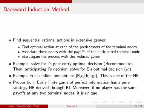
Backward Induction Method

Find sequential rational actions in extensive games:

Find optimal action at each of the predecessors of the terminal nodesAssociate these nodes with the payo¤s of the anticipated terminal nodeStart again the process with this reduced game

Example: solve for I�s post-entry optimal decision (Accommodate).Then, anticipating I�s decision, solve for E�s optimal decision (In)

Example in next slide: one obtains [R,c,(b,f,g)]. This is one of the NE.

Proposition: Every �nite game of perfect information has a purestrategy NE derived through BI. Moreover, if no player has the samepayo¤s at any two terminal nodes, it is unique


Another Example


Solving by Backwards Induction


Subgame Perfect Nash Equilibrium: Example

Extension of backwards induction to �imperfect information�games


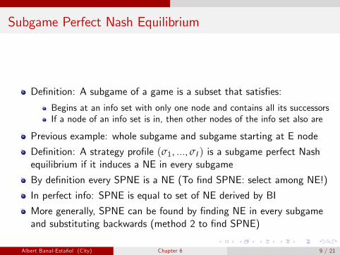
Subgame Perfect Nash Equilibrium

De�nition: A subgame of a game is a subset that satis�es:

Begins at an info set with only one node and contains all its successorsIf a node of an info set is in, then other nodes of the info set also are

Previous example: whole subgame and subgame starting at E node

De�nition: A strategy pro�le (σ1, ..., σI ) is a subgame perfect Nashequilibrium if it induces a NE in every subgame

By de�nition every SPNE is a NE (To �nd SPNE: select among NE!)

In perfect info: SPNE is equal to set of NE derived by BI

More generally, SPNE can be found by �nding NE in every subgameand substituting backwards (method 2 to �nd SPNE)


Example (continued)

Normal form:

EnI A if In F if InOut, A if In 0,2 0,2Out, F if In 0,2 0,2In, A if In 3,1 -2,-1In, F if In 1,-2 -3,-1

NE:

Do all of them induce a NE in every subgame? SPNE:

Other examples in Industrial Organisation: choosing degree ofdi¤erentiation before competing in prices


6.2.- More Games

Stackelberg competition:

Model, representation and backwards inductionOutcome and comparison with Cournot

Another model of entry:

Model, representation and SPNE


Stackelberg Competition: Model

As in the Cournot model, two �rms select quantities and...an auctioneer chooses the price according to P() where

P(q1 + q2) =�1� (q1 + q2) if q1 + q2 � 10 if q1 + q2 > 1

and each �rm�s unit costs are c (� 1)But now...

Firm 1 sets its output before Firm 2 doesFirm 2 observes Firm 1�s output, q1, before choosing q2


Stackelberg Competition: Elements

Players: Firms 1 and 2. Payo¤s:

Πi (qi , qj ) = (maxf[1� (qi + qj )] , 0g) qi � cqi

Strategy for 1: an output q1 2 [0,∞)Strategy for 2: a function q2(q1), i.e. an output [0,∞) for each q1Examples of strategies:

q1 = 0.5

q2(q1) = 3q1 for any q1


(Approximate) representation:


Stackelberg Competition: Backwards Induction (BI)

Solving by backwards induction, Firm 2�s best reply (FOC) is:

q�2 (q1) = B2(q1) =� 1�q1�c

2 if q1 � 1�c2

0 if q1 > 1�c2

Anticipating this, Firm 1 maximises (clearly q�1 � 1�c2 )

Π1(q1,B2(q1)) =�1�

�q1 +

1� q1 � c2

��q1 � cq1

Solving the FOC:

q�1 =1� c2

The NE obtained by BI is given by (q�1 , q�2 (q1))


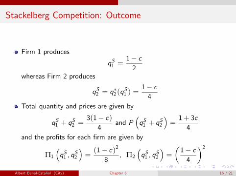
Stackelberg Competition: Outcome

Firm 1 produces

qS1 =1� c2

whereas Firm 2 produces

qS2 = q�2 (q

S1 ) =

1� c4

Total quantity and prices are given by

qS1 + qS2 =

3(1� c)4

and P�qS1 + q

S2

�=1+ 3c4

and the pro�ts for each �rm are given by

Π1

�qS1 , q

S2

�=(1� c)2

8, Π2

�qS1 , q

S2

�=

�1� c4

�2Albert Banal-Estañol (City) Chapter 6 16 / 21

Stackelberg vs Cournot

Firm 1 produces more than in Cournot

qS1 =1� c2

>1� c3

= qC1

whereas Firm 2 produces less

qS2 =1� c4

<1� c3

= qC2

Firm 1 earns more than in Cournot

ΠS1 =

(1� c)2

8>(1� c)2

9= ΠC

1

whereas Firm 2 earns less

ΠS2 =

(1� c)2

16>(1� c)2

9= ΠC

2


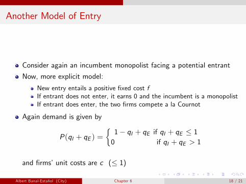
Another Model of Entry

Consider again an incumbent monopolist facing a potential entrant

Now, more explicit model:

New entry entails a positive �xed cost fIf entrant does not enter, it earns 0 and the incumbent is a monopolistIf entrant does enter, the two �rms compete a la Cournot

Again demand is given by

P(qI + qE ) =�1� qI + qE if qI + qE � 10 if qI + qE > 1

and �rms�unit costs are c (� 1)


Entry Model: Elements

Players: Firms I and E

Strategies: E : fIn or Out, qE g; I : fqI g where qE , qI 2 [0,∞)Payo¤s (if the entrant enters):

ΠI (In, qE , qI ) = (maxf1� (qE + qI ), 0g) qI � cqIΠE (In, qE , qI ) = (maxf1� (qE + qI ), 0g) qE � cqE � f

Payo¤s (if the entrant does not enter):

ΠI (Out, qI ) = (maxf1� qI , 0g) qI � cqIΠE (Out, qI ) = 0


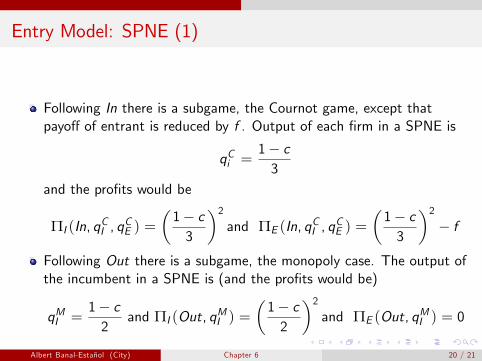
Entry Model: SPNE (1)

Following In there is a subgame, the Cournot game, except thatpayo¤ of entrant is reduced by f . Output of each �rm in a SPNE is

qCi =1� c3

and the pro�ts would be

ΠI (In, qCI , q

CE ) =

�1� c3

�2and ΠE (In, q

CI , q

CE ) =

�1� c3

�2� f

Following Out there is a subgame, the monopoly case. The output ofthe incumbent in a SPNE is (and the pro�ts would be)

qMI =1� c2

and ΠI (Out, qMI ) =

�1� c2

�2and ΠE (Out, q

MI ) = 0


Entry Model: SPNE (2)

Anticipating this, in a SPNE the potential entrant enters whenever

ΠE (In, qCI , q

CE ) =

�1� c3

�2� f � 0 = ΠE (Out, q

MI )

In sum, the outcome of the SPNE of the game depend on f and c :If f <

� 1�c3

�2: (one SPNE) In and qi = qCi =

1�c3 for i = E , I

If f >� 1�c3

�2: (one SPNE) Out and qI = qMI =

1�c2

If f =� 1�c3

�2: (two SPNE) the two previous outcomes may arise

Notice that, as before, there is a NE (not SPNE) in which theincumbent �oods the market and the potential entrant does not enter


chapter 6: dynamic games - albert...

Documents