chapter 6 the guide approach to subgroup identiﬁcation

Chapter 6The GUIDE Approach to SubgroupIdentification

Wei-Yin Loh and Peigen Zhou

Abstract GUIDE is a multi-purpose algorithm for classification and regression treeconstruction with special capabilities for identifying subgroups with differentialtreatment effects. It is unique among subgroup methods in having all thesefeatures: unbiased split variable selection, approximately unbiased estimation ofsubgroup treatment effects, treatments with two or more levels, allowance forlinear effects of prognostic variables within subgroups, and automatic handling ofmissing predictor variable values without imputation in piecewise-constant models.Predictor variables may be continuous, ordinal, nominal, or cyclical (such as angularmeasurements, hour of day, day of week, or month of year). Response variablesmay be univariate, multivariate, longitudinal, or right-censored. This article gives acurrent account of the main features of the method for subgroup identification andreviews a bootstrap method for conducting post-selection inference on the subgrouptreatment effects. A data set pooled from studies of amyotrophic lateral sclerosis isused for illustration.

Keywords Bootstrap · Classification and regression tree · Confidence interval ·Missing value · Post selection inference · Recursive partitioning · Variableselection

6.1 Introduction

GUIDE (Loh 2002, 2009) is an algorithm for fitting classification and regressiontree models to data. AID (Morgan and Sonquist 1963) was the first algorithm butCART (Breiman et al. 1984) and RPART (Therneau and Atkinson 2018) brought thebasic ideas to the mainstream. GUIDE grew out of work on an alternative approachto CART classification (Loh and Vanichsetakul 1988; Loh and Shih 1997; Kim and

W.-Y. Loh (�) · P. ZhouDepartment of Statistics, University of Wisconsin, Madison, WI, USAe-mail: [email protected]; [email protected]

© Springer Nature Switzerland AG 2020N. Ting et al. (eds.), Design and Analysis of Subgroups with BiopharmaceuticalApplications, Emerging Topics in Statistics and Biostatistics,https://doi.org/10.1007/978-3-030-40105-4_6

147

http://crossmark.crossref.org/dialog/?doi=10.1007/978-3-030-40105-4_6&domain=pdf

mailto:[email protected]

mailto:[email protected]

https://doi.org/10.1007/978-3-030-40105-4_6

148 W.-Y. Loh and P. Zhou

Loh 2001, 2003) and regression (Loh 1991b; Ahn and Loh 1994; Chaudhuri et al.1994, 1995; Chaudhuri and Loh 2002; Chan and Loh 2004). See Loh (2014) for arecent review of classification and regression trees. Unlike AID and CART that onlyfit a constant in each node of the tree, GUIDE can fit linear and generalized linearmodels. This makes GUIDE well suited for subgroup identification—the terminalnodes of the tree are the subgroups and the regression coefficients in the node modelsgive the treatment effects. It is unique among subgroup methods in having propertiessuch as unbiased selection of split variables, approximately unbiased estimationof treatment effects, ability to use treatment variables with more than two levels,optional local adjustment for linear effects of prognostic variables, and automatichandling of missing values without needing prior imputation. Predictor variablesmay be continuous, ordinal, nominal, or cyclical (such as angles, hour of day, dayof week, and month of year). Response variables may be univariate, multivariate,longitudinal, or right censored. Missing values may be coded in more than oneway; for example a missing value for age of spouse may be coded as “refuse toanswer” if the respondent did not provide an answer and as “valid nonresponse”if the respondent is single, widowed or divorced; see Loh et al. (2019b) for otherexamples.

This article gives a current account of the GUIDE method for subgroupidentification. It uses data combined from several studies of ALS (AmyotrophicLateral Sclerosis) for illustration. The data were selected because they containedall of the types of response variables that GUIDE can model and because manyof the predictor variables had missing values (denoted by “NA” here). ALS isa neurological disease that affects voluntary muscle movement. Death typicallyoccurs within 3–5 years of diagnosis. Only about a quarter of patients survive formore than 5 years after diagnosis. The data were obtained from the Pooled ResourceOpen-Access ALS Clinical Trials (PRO-ACT) Database (Atassi et al. 2014). In2011, Prize4Life, in collaboration with the Northeast ALS Consortium, and withfunding from the ALS Therapy Alliance, formed the PRO-ACT Consortium. Thedata in the PRO-ACT Database were provided by the PRO-ACT Consortiummembers. They were pooled from 23 completed ALS clinical trials and oneobservational study, and contained information on demographics, family history,and clinical and laboratory test data from more than 10700 ALS patients.

The ALS Functional Rating Scale (ALSFRS) is often used to evaluate thefunctional status of ALS patients. It is the sum of ten scores (speech, salivation,swallowing, handwriting, cutting food and handling utensils, dressing and hygiene,turning in bed and adjusting bed clothes, walking, climbing stairs, and breathing),with each score measured on a scale of 0–4, with 4 being normal. Seibold et al.(2016) used a subset of the data to study the effectiveness of riluzole, a drugapproved for treatment of ALS by the US FDA, on ALSFRS at 6 months as well assurvival time from trial enrollment. Using the MOB algorithm (Zeileis et al. 2008),they found that for patients with less than 468 days between disease onset and startof treatment, riluzole had a negative treatment effect on ALSFRS at 6 months.

A major difficulty with the PRO-ACT data is that besides riluzole, othermedications were also tested in many of the trials (Atassi et al. 2014, Table 1).

6 GUIDE Approach 149

Even worse, the additional medications were not identified in the data. To avoidconfounding the effects of riluzole and that of other medications, the analysishere is restricted to the subset of 1270 subjects who were assigned to placeboor riluzole only, without other medications. Thirty-six variables were chosen aspredictor variables; their names are given in Table 6.1 together with their minimumand maximum values and numbers of missing values. Three additional variableswere chosen as dependent variables: (1) change in ALSFRS from baseline at 6months, (2) monthly change in ALSFRS from baseline at months 1, 2, . . . , 6, and(3) survival time in days. ALSFRS scores of subjects who had died by the time thescores were to be measured were set to 0. ALSFRS variables at 0, 1, . . . , 6 monthsare denoted by ALSFRS0, ALSFRS1, . . . , ALSFRS6, respectively.

6.2 Univariate Uncensored Response

Figure 6.1 shows a basic GUIDE tree for predicting change in ALSFRS after6 months (ALSFRS6 minus ALSFRS0), where a linear model (6.1) with treatmentas the only predictor variable is fitted in each node. A node of the tree representsa partition of the data, with the root node corresponding to the whole data set. Thesample size in each partition is printed beside the node. At each node, a variable X

is selected to split the data there into two child nodes. The split, in the form X ∈ A,is printed on the left of the node. The set A is chosen to minimize the sum of thesquared residuals in the left and right child nodes. Observations in the node are sentto the left child node if and only if the condition is satisfied. Node labels start with1 for the root node; for a node with label k, its left and right child nodes are labeled2k and 2k + 1, respectively.

The root node in Fig. 6.1 is split on Diagnosis_Delta, which is the numberof days from clinical diagnosis to the first time the subject was tested in a trial. The239 subjects with missing values in Diagnosis_Delta go to terminal node 2 andthe others go to intermediate node 3. It is unknown why the subjects have missingvalues in Diagnosis_Delta. One possibility is the variable was not measuredin some of the trials, but this cannot be verified because trial ID was not included inthe data. Nevertheless, as the barplot for node 2 in Fig. 6.1 shows, subjects in thissubgroup deteriorate much more on average with riluzole than without. Subjects innode 3 are split on Hematocrit. Those with Hematocrit missing or ≤ 37.95(abbreviated in the tree diagrams by the symbol “≤∗” with the asterisk standing for“is missing”) go to node 6 where they are split on BP_Diastolic and then onPotassium.

6.2.1 Node Models

Let X = (X1, X2, . . . , XK) denote a K-dimensional vector of covariates, Y aunivariate response variable, and Z a treatment variable taking values 0, 1, . . . ,G,


Table 6.1 Predictor variables, minimum and maximum values, numbers of categorical levels, andnumbers of missing values for modeling the difference ALSFRS6-ALSFRS0

Name Definition Min Max Miss

Demographics_Delta Demographic measurement day −35.00 32.00 19

Age Subject age at start of trial 18.00 82.00

Sex Subject gender (female, male)

Race Subject race (5 categories) 3

ALS_History_Delta Day ALS history reported 0.00 3.00 43

Symptom Major symptom (10 categories) 1085

Onset_Delta Day of disease onset, from first test −1900.00 −84.00 47

Diagnosis_Delta Day of diagnosis, from first test −1666.00 0.00 239

Site_of_Onset Site of disease onset (3 categories)

Albumin Albumin in blood (g/L) 31.67 53.00 332

ALT_SGPT Alanine amino transferase (U/L) 6.00 181.00 259

AST_SGOT Aspartate amino transferase (U/L) 7.50 116.00 258

Basophil_Count Amount in white blood cell (×109/L) 0.00 5.56 341

Basophils Percent in white blood cell count 0.00 3.00 365

Blood_Urea_Nitrogen Ureas (mmol/L) 0.95 17.34 218

Calcium Calcium in metabolic panel (mmol/L) 1.55 3.00 333

Creatinine Creatinine from kidney test 25.00 159.10 216

Eosinophils Percent in white blood cell count 0.00 15.00 365

Glucose Glucose in blood (mmol/L) 0.07 18.56 325

Hematocrit Percent red blood cells 0.00 56.00 326

Hemoglobin Hemoglobin in blood (g/L) 94.50 181.00 326

Lymphocytes Percent lymphocyte in blood 8.70 50.00 365

Monocytes Percent in white blood cell count 0.00 21.40 365

Platelets Platelets in blood (×109/L) 0.20 552.00 332

Potassium Potassium in electrolytes (mmol/L) 3.30 5.50 258

Sodium Sodium in electrolytes (mmol/L) 125.00 150.00 257

Urine_Ph Acidity of urine 5.00 9.00 355

SVC(Slow_vital_Capacity)

Volume of air exhaled slowly (L) 1.00 7.00 737

Slow_vital_Capacity_Delta

Day of SVC assessment 0.00 14.00 737

BP_Diastolic Diastolic blood pressure (mmHg) 52.00 125.00 217

BP_Systolic Systolic blood pressure (mmHg) 90.00 200.00 217

Height Subject height (in) 131.00 205.00 225

Pulse Beats per minute 42.00 120.00 218

Weight Subject weight (kg) 38.33 138.20 178

ALSFRS0 ALSFRS at baseline 10.00 40.00

ALSFRS_Delta0 Day of ALSFRS0 measurement −7.00 154.00

Variables with names containing “_Delta” are days from trial onset to the date that an assessmenttook place, with negative values for occurrences before trial onset


Diagnosis_Delta= NA 1

239 2

(-18.6, -8.8)

Hematocrit≤∗37.95 3

BP_Diastolic≤∗55.50 6

179 12

(-4.7, 3.6)

Potassium≤∗3.37 13

75 26

(-26.8, 2.2)

27

(-9.4, 3.3)

170

7

(-1.5, 9.1)

607

Placebo Riluzole

Node 2

Mea

n ch

ange

in A

LSF

RS

−25

−20

−15

−10

−5

0

Placebo Riluzole

Node 7

−25

−20

−15

−10

−5

0

Placebo Riluzole

Node 12

−25

−20

−15

−10

−5

0

Placebo Riluzole

Node 26

Mea

n ch

ange

in A

LSF

RS

−25

−20

−15

−10

−5

0

Placebo Riluzole

Node 27

−25

−20

−15

−10

−5

0

Fig. 6.1 GUIDE tree for change in ALSFRS (ALSFRS6-ALSFRS0) using 1270 observations andnode model (6.1). At each split, an observation goes to the left branch if and only if the condition issatisfied. The symbol “≤∗” stands for “≤ or missing.” Sample sizes (in italics) are printed besidenodes. Bootstrap-calibrated 90% simultaneous intervals of treatment effect are given below nodes.Calibrated alpha is 1.3 × 10−5. Treatment effect is statistically significant in green node. Barplotsshow means of change in ALSFRS for placebo and riluzole subjects in the terminal nodes


with 0 being the reference (or placebo) level. Let t denote a node of the tree. Aregression tree model is constructed by recursively partitioning a training sampleinto subsets that are represented by the nodes of a tree. A large majority ofregression tree methods for subgroup identification employ stopping rules basedon Bonferroni-corrected p-values (Lipkovich et al. 2011; Seibold et al. 2016; Suet al. 2009). Other methods (Dusseldorp and Meulman 2004; Foster et al. 2011),including GUIDE, first grow an overly large tree and then use cross-validation toprune it to a smaller size. We only describe the GUIDE node fitting and splittingsteps here because the pruning step is the same as that of CART.

For least-squares regression, GUIDE fits a linear model Y = f (X, Z) + ε tothe data in each node of a tree; ε is an independent zero-mean random variable withvariance that is constant within each node but may vary between nodes. Four choicesof f (x, z) are available, depending on the number of X variables to be included. Letβz (z = 1, 2, . . . ,G) denote the effect of treatment level z (versus level 0). Thechoices are:

f (x, z) = η + βz (Treatment only) (6.1)

f (x, z) = η + βz +p∑

j=1

γjxjk∗ (Polynomial of degree p) (6.2)

f (x, z) = η + βz +K∑

k

γkxk (Multiple linear) (6.3)

f (x, z) = η + βz +∑

k∈Sγkxk (Stepwise linear) (6.4)

In (6.2), p is a user-specified positive integer and k∗ is the value of k such thatXk minimizes the sum of squared residuals in the node (k∗ may vary from node tonode). In (6.4), the set S is the set of indices of the variables Xk that are selectedby forward and backward stepwise regression in the node. Thus the model for a treewith terminal nodes t1, t2, . . . , tτ may be written as

Y =

⎧⎪⎨

⎪⎩

f1(X, Z) + ε1, X ∈ t1...

fτ (X, Z) + ετ , X ∈ tτ

(6.5)

where f1, f2, . . . , fτ take one of the functional forms (6.1)–(6.4) and ε1, . . . , ετare independent random variables with mean zero and variances σ 2

1 , . . . , σ2τ . This is

different from the model

Y =τ∑

j=1

fj (X, Z) I (X ∈ tj ) + ε (6.6)


which assumes that the error variance is the same in all nodes. The least-squaresestimates of the regression coefficients are the same in models (6.5) and (6.6), butnot their standard error estimates. In (6.2)–(6.4), missing values in the X variablesare imputed by their node means.

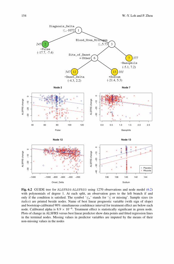
Figure 6.1 was constructed using model (6.1) and Fig. 6.2 was constructed usingmodel (6.2) with p = 1. The name of the best linear prognostic variable Xk∗ isgiven beneath each terminal node. The root node splits on “Diagnosis_Delta≤ − 1072 or missing.” Of the 245 subjects in this subgroup, 239 are missingDiagnosis_Delta. The best linear prognostic variable in node 2 is Pulse.Plots of the data and regression lines for placebo and riluzole subjects in each nodeare shown in the lower half of Fig. 6.2. Mean imputation of Sodium is clearlyshown by the vertical line of points in the plot of node 13.

6.2.2 Split Variable Selection

To find a variable to split a node t , a test of treatment-covariate interaction isperformed for each Xk on the data in t . (This is the default “Gi” method.) Let ntdenote the number of observations in t . The following steps are carried out for eachvariable Xj , j = 1, 2, . . . , K .

1. If Xj is a categorical variable, define V = Xj and let h denote its number oflevels (including a level for NA, if any).

2. If Xj is ordinal and takes only one value (including NA) in the node, do not use itto split the node. Otherwise, let m denote the number of distinct values (includingNA) of Xj in t . Transform it to a discrete variable V with h values as follows.

(a) If m ≤ 4 or if m = 5 and Xj has missing values, define h = m. Otherwise,define h = 3 if nt < 30(G + 1) and h = 4 otherwise.

(i) If Xj has missing values in t , define rk = k/(h−1), k = 1, 2, . . . , h−2.(ii) If Xj has no missing values in t , define rk = k/h, k = 1, 2, . . . , h − 1.

(b) Define q0 = −∞ and let qk (k > 0) be the sample rk-quantile of Xj in t .

(i) If Xj has missing values in t , define

V =h−2∑

k=1

kI (qk−1 < Xj ≤ qk)+(h−1)I (Xj > qh−2)+hI (Xj = NA).

(ii) If Xj has no missing values in t , define

V =h−1∑

k=1

kI (qk−1 < Xj ≤ qk) + hI (Xj > qh−1).


Diagnosis_Delta

≤∗-1072 1

245 2-Pulse

(-17.7, -7.4)

Blood_Urea_Nitrogen

≤∗5.73 3

Site_of_Onset= Other 6

547 12-Onset_Delta(-4.3, 2.2)

13 101+Sodium(-21.4, 5.3)

7 377-Basophils

(-5.1, 7.2)

40 60 80 100 120

−30

−20

−10

0

Pulse

ALS

FR

S c

hang

e

Node 2

0.0 0.5 1.0 1.5 2.0 2.5

−30

−20

−10

0

Basophils

ALS

FR

S c

hang

e

Node 7

−1400 −1000 −800 −600 −400 −200

−30

−20

−10

0

Onset_Delta

ALS

FR

S c

hang

e

Node 12

136 138 140 142 144

−40

−30

−20

−10

0

Sodium

ALS

FR

S c

hang

e

PlaceboRiluzole

Node 13

Fig. 6.2 GUIDE tree for ALSFRS6-ALSFRS0 using 1270 observations and node model (6.2)with polynomials of degree 1. At each split, an observation goes to the left branch if andonly if the condition is satisfied. The symbol ‘≤∗’ stands for ‘≤ or missing’. Sample sizes (initalics) are printed beside nodes. Name of best linear prognostic variable (with sign of slope)and bootstrap-calibrated 90% simultaneous confidence interval for treatment effect are below eachnode. Calibrated alpha is 8.9 × 10−6. Treatment effect is statistically significant in green node.Plots of change in ALSFRS versus best linear predictor show data points and fitted regression linesin the terminal nodes. Missing values in predictor variables are imputed by the means of theirnon-missing values in the nodes


3. Test the additive model E(Y |Z,V ) = η +∑z βzI (Z = z) +∑v γvI (V = v),with β0 = γ1 = 0, against the full model E(Y |Z,V ) = ∑

z

∑v ωvzI (V =

v, Z = z) and obtain the p-value pj .

Split node t on the Xj with the smallest value of pj .

6.2.3 Split Set Selection

After X is selected, a search is carried out for the best split “X ∈ A”, where A

depends on whether X is ordinal or categorical.

6.2.3.1 Ordinal Variable

If X is ordinal, three types of splits are evaluated.

1. X = NA: an observation goes to the left node if and only if its value is missing.2. X = NA or X ≤ c: an observation goes to the left node if and only if its value is

missing or if it is less than or equal to c.3. X ≤ c: an observation goes to the left node if and only if its value is not missing

and it is less than or equal to c.

Candidate values of c are the midpoints between consecutive order statistics of Xin t . If X has m order statistics, the maximum number of possible splits is (m − 1)or {1 + 2(m − 1)}, depending on the absence or presence of missing X values in t .Permissible splits are those that yield two child nodes with each having two or moreobservations per treatment. The selected split is the one that minimizes the sum ofthe deviances (or sum of squared residuals in the case of least-squares regression)in the two child nodes.

This method of dealing with missing values is unique to GUIDE. CART usesa hierarchical system of “surrogate splits” on alternative X variables to sendobservations with missing values to the child nodes. Because the surrogate splitsdepend on the (missing and non-missing) values of the alternative X variables,observations with missing values do not necessarily go to the same child node.Therefore it is impossible to predict the path of an observation by looking at the treewithout knowing the values of its predictor variables. Besides, CART’s surrogatessplits are biased towards X variables with few missing values (Kim and Loh 2001).Other subgroup methods are typically inapplicable to data with missing values(Dusseldorp and Meulman 2004; Su et al. 2009; Foster et al. 2011; Seibold et al.2016).

Sometimes, missing-value imputation is illogical, e.g., a prostate-specific antigentest result for a female subject or the age of first cigarette for a subject who neversmoked. Other times, imputation erases useful information. For example, if missingvalues were imputed before application of GUIDE, the large difference in treatmenteffect between subjects with and without missing values in Diagnosis_Deltain Fig. 6.1 would be undetected.


6.2.3.2 Categorical Variable

If X is a categorical variable, the split has the form X ∈ A, where A is a non-trivialsubset of the values (including NA) of X in t . A complete search of all possiblevalues of A can be computationally expensive if the number, m, of distinct values(including NA) of X in t is large, because there are potentially (2m−1 −1) splits (lessif some splits yield child nodes with fewer than two observations per treatment).Therefore GUIDE carries out a complete search only if m ≤ 11. If m > 11, itperforms an approximate search by means of linear discriminant analysis , basedon an idea from Loh and Vanichsetakul (1988), Loh and Shih (1997), and Loh(2009).

1. Let yz denote the sample mean of the Y values in t that belong to treatment Z = z

(z = 0, 1, . . . ,G).2. Define the class variable

C ={

2z − 1, if Z = z and Y > yz

2z, if Z = z and Y ≤ yz.

3. Let {a1, a2, . . . , am} denote the categorical values of X in t . Transform X to anm-dimensional 0–1 dummy vector D = (D1,D2, . . . , Dm), where Di = I (X =ai), i = 1, 2, . . . , m.

4. Apply linear discriminant analysis to the data (D, C) in t to find the discriminantvariables Bj = ∑m

i=1 bijDi , j = 1, 2, . . .. These variables are also calledcanonical variates (Gnanadesikan 1997).

5. For each j , find the split Bj ≤ cj that minimizes the sum of the squared residualsof the least-squares models fitted in the child nodes induced by the split.

6. Let j∗ be the value of j for which Bj ≤ cj has a smallest sum of squaredresiduals.

7. Split the node with Bj∗ ≤ cj∗ . Because Bj∗ =∑mi=1 bij∗Di =∑m

i=1 bij∗I (X =ai), the split is equivalent to X ∈ A with A = {ai : bij∗ ≤ cj∗}.

6.3 Bootstrap Confidence Intervals

The barplots in the lower half of Fig. 6.1 show that the subgroups defined by nodes 2and 26 have the largest treatment effects. Similarly, the graphs in the lower halfof Fig. 6.2 suggest that node 2 has the largest treatment effect. Are the effectsstatistically significant? This question cannot be answered by means of traditionalmethods because the subgroups were not specified independently of the data. It is aquestion of post-selection inference.

Given node t and z, let β(t, z) be the estimated treatment effect for Z = z in t , letσβ(t, z) denote its usual estimated standard error, and let νt be the residual degreesof freedom. Further, let tν,α denote the (1 − α)-quantile of the t-distribution with ν

degrees of freedom and let τ denote the number of terminal nodes of the tree. Let


Table 6.2 90% simultaneousintervals for subgrouptreatment effects in Figs. 6.1and 6.2

Model Node B(0.10, t, z) J (αF

, t, z)

Figure 6.1 2 (−16.0,−11.4) (−18.7,−8.7)

αF

= 1.3 × 10−5 7 (1.3, 6.3) (−1.6, 9.2)

12 (−2.5, 1.4) (−4.7, 3.6)

26 (−18.7,−5.8) (−26.2, 1.7)

27 (−6.0,−0.1) (−9.4, 3.3)

Figure 6.2 2 (−15.1,−10.0) (−17.7,−7.4)

αF

= 8.9 × 10−6 7 (−2.1, 4.1) (−5.1, 7.2)

12 (−2.7, 0.6) (−4.3, 2.2)

13 (−14.5,−1.6) (−21.4, 5.3)

B(α, t, z) = β(t, z) ± tνt ,α/(2τ) σβ(t, z) (6.7)

be the Bonferroni-corrected 100(1 − α)% simultaneous t-interval for the treatmenteffect of Z = z in node t . The middle column of Table 6.2 gives the values ofB(0.10, t, z) for the trees in Figs. 6.1 and 6.2. Despite the Bonferroni correction,the standard errors σβ(t, z) are biased low because they do not account for theuncertainty due to split selection. As a result, the intervals B(α, t, z) tend to betoo short and their simultaneous coverage probability is less than (1 − α).

There are two obvious ways to lengthen the interval widths to improve theircoverage probabilities. One is to correct the standard error estimates, but this isformidable due to the complexity of the tree algorithm. Another way is to reducethe nominal value of α in (6.7). For example, to obtain 90% simultaneous coverage,we could use B(α, t, z) with a nominal α < 0.10. To find the right nominal valueof α, we first need to define the estimand of β(t, z), which is the true treatmenteffect in t . Let F denote the training data and F the population from which theyare drawn. By definition, β(t, z) (z = 1, . . . ,G) are the values of the treatmenteffect coefficients that minimize

∑i∈t (yi − f (xi , zi))2, where the sum is over the

observations in node t . Their estimands, denoted by are βF (t, z), are the values ofthe treatment effect coefficients that minimize E{(Y −f (X, Z))2I (X ∈ t)}. Clearly,βF (t, z) is a random variable, because it depends on t , which in turn depends on F .If F is known and t is given, however, βF (t, z) can be computed, by simulationfrom F if necessary.

Let J (α, t, z) = β(t, z) ± tνt ,α/2 σβ(t, z) denote the nominal 100(1 − α)% t-interval, let T be the set of terminal nodes, and let γF (α) = P [∩

t∈T {βF (t, z) ∈J (α, t, z)}] denote the simultaneous coverage probability. Clearly, γF (α) ↑ 1 asα ↓ 0. Given a desired simultaneous coverage probability γ ∗, let αF be thesolution of the equation γF (αF ) = γ ∗. Then the intervals J (αF , t, z) have exactsimultaneous coverage γ ∗. We call αF the “calibrated α.” Note that there is no needto work with the Bonferroni-corrected interval (6.7) because γF (α) is, by definition,a simultaneous coverage probability.

Of course, the value of αF is not computable if F is unknown. In that case, anatural solution is bootstrap calibration, a method proposed in Loh (1987, 1991a)for the simpler problem of estimating a population mean. It was extended to


Algorithm 1: Bootstrap calibration of confidence intervals for treatment effectsData: Given K > 0 and α ∈ (0, 1), α1 < α2 < . . . < αK = α; tree T with nodes

t1, t2, . . . , tL constructed from D = {(Xi , Yi , Zi), i = 1, 2, . . . , n}; and model M(one of (6.1), . . . , or (6.4)) based on T with estimated treatment effects βtz,z = 1, 2, . . . ,G; t = t1, t2, . . . , tL.

Result: (1 − α) simultaneous t-intervals for {βtz}.begin

γk ← 0 for k = 1, 2, . . . , K;for b ← 1 to B do

bootstrap data D∗b = {(X∗

i , Y∗i , Z

∗i ), i = 1, 2, . . . , n} from D ;

construct from D∗b tree Tb with nodes t∗b1, t

∗b2, . . . , t

∗bLb

;fit model M based on Tb to D observations to get ‘‘true’’ effects β(t∗bl , z);z = 1, . . . ,G; l = 1, . . . , Lb;

fit model M based on Tb to D∗b observations to get estimates β(t∗bl , z), residual

degrees of freedom νbl and standard errors σβ (t∗bl , z); z = 1, . . . ,G; l = 1, . . . , Lb;for z ← 1 to G do

for l ← 1 to Lb dofor k ← 1 to K do

Jklz ← (1 − αk) t-interval β(t∗bl , z) ± tνbl ,αk/2σβ (t∗bl , z);

if β(t∗bl , z) ∈ Jklz thencklz ← 1 ; /* interval contains true beta */

elsecklz ← 0 ; /* interval does not contain truebeta */

endend

endendfor k ← 1 to K do

if minlz cklz = 1 thenγk ← γk + 1

endend

endγk ← γk/B for k = 1, 2, . . . , K;q ← smallest k such that γk < 1 − α;g ← (γq−1 − 1 + α)/(γq−1 − γq);α′ ← (1 − g)αq−1 + gαq ;construct (1 − α′) simultaneous t-intervals for βtz for t = t1, t2, . . . , tL; z = 1, . . . ,G

end

estimation of subgroup treatment effects in Loh et al. (2016, 2019c). The idea isto replace F with F in the calculations. Specifically, use simulation from F to findthe solution α

Fof the equation γ

F(α

F) = γ ∗. The resulting intervals J (α

F, t, z)

are called “bootstrap-calibrated” 100γ ∗% simultaneous intervals. Algorithm 1 givesthe instructions in pseudo-code, using a grid search to find α

F. The numerical

results here (including those in the last column of Table 6.2) were obtained witha grid of 200 nominal values of α and 1000 bootstrap iterations. Simultaneous


90% bootstrap-calibrated intervals of treatment effect are given beneath the terminalnodes of the trees in Figs. 6.1 and 6.2. Their respective bootstrap-calibrated alphavalues are α

F= 1.3 × 10−5 and 8.9 × 10−6. In the tree diagrams, nodes with

statistically significant treatment effects are in green color.

6.4 Multivariate Uncensored Responses

GUIDE can construct a least-squares regression tree for data with longitudinal ormultivariate response variables as well. Given d response variables Y1, Y2, . . . , Yd ,it fits the treatment-only model E(Yj |Z) = ηj + ∑G

z=1 βjzI (Z = z), j =1, . . . , d, separately to each variable in each node. To find the variable to splita node, the test for treatment-covariate interaction in Sect. 6.2.2 is performed d

times for each Xi (once for each Yj ) to obtain the p-value pi1, pi2, . . . , pid . Letχ2ν,α denote the (1 − α)-quantile of the chi-squared distribution with ν degrees

of freedom. The variable Xi for which∑d

j=1 χ21,pij

is maximum is selected tosplit the node. To allow for correlations in the response variables, GUIDE canoptionally apply the treatment-covariate interaction tests to the principal component(PC) or linear discriminant (LD) variates computed from the Yj values in the node.Specifically, if principal component transformation is desired, the (Y1, Y2, . . . , Yd)

data vectors in the node are transformed to their PCs (Y ′1, Y

′2, . . . , Y

′d) first; then

the treatment-covariate interactions tests are applied to the (Y ′1, Y

′2, . . . , Y

′d) data

vectors. Similarly, if LD is desired, the (Y1, Y2, . . . , Yd) data vectors in the node aretransformed to their linear discriminant variates, using the treatment levels as classlabels. The PC and LD transformations are carried out locally at each node. Afterthe split variable Xi is selected, its split point (if Xi is ordinal) or split set (if Xi

is categorical) is the value that yields the smallest total sum of squared residuals(where the total is over the d models E(Yj |Z) = ηj +∑z βjzI (Z = z)) in the leftand right child nodes. See Loh and Zheng (2013) and Loh et al. (2016) for moredetails.

Using change from baseline of ALSFRS1, ALSFRS2, . . . , ALSFRS6 as longi-tudinal response variables, only the PC option yielded a nontrivial tree, as shown inFig. 6.3. Subjects who died after 6 months and had missing values in any responsevariable were omitted, leaving a training sample of 627 observations. The treehas only one split, the same as the split at the root node of Fig. 6.2. The plotsbelow the tree diagram show bootstrap-calibrated 90% simultaneous intervals forthe treatment effect for each response variable in each terminal node. The longerlengths of the intervals in the left node are due to its much smaller sample size.Because every interval contains 0, there is no subgroup with statistically significanttreatment effect.


Diagnosis_Delta

≤∗-1072 1

2

33

3

594

1 2 3 4 5 6

−20

−10

010

20

Month from trial onset

Cal

ibra

ted

90%

sim

ulta

neou

s in

terv

als

for

trea

tmen

t effe

ct

−

−

−

−

−

−

−

−

−

−

−

−

Diagnosis_Delta ≤ − 1072 or NA

1 2 3 4 5 6

−20

−10

010

20

Month from trial onset

Cal

ibra

ted

90%

sim

ulta

neou

s in

terv

als

for

trea

tmen

t effe

ct−− −

−−−

−

−−

−

−

−

Diagnosis_Delta > − 1072

Fig. 6.3 GUIDE tree for change from baseline of longitudinal responses ALSFRS1, ALSFRS2,. . . , ALSFRS6, using 627 observations and PCA at each node. At each split, an observation goes tothe left branch if and only if the condition is satisfied. The symbol ‘≤∗’ stands for ‘≤ or missing’.Sample size (in italics) printed below nodes. Bootstrap-calibrated 90% simultaneous intervals fortreatment effect of each response variable in each node plotted below tree. Calibrated alpha is 0.011

6.5 Time-to-Event Response

Let (U1,X1), (U2,X2), . . . , (Un,Xn) be the survival times and predictor variablevalues of n subjects. Let V1, V2, . . . , Vn be independent and identically distributedobservations from a censoring distribution and let δi = I (Ui < Vi) be theevent indicator. The observed data vector of subject i is (Yi, δi ,Xi ), where Yi =min(Ui, Vi). Let λ(y, x, z) denote the hazard function at time y and covariates xand z. The proportional hazards model stipulates that λ(y, x, z) = λ0(y) exp(η),where λ0(y) is a baseline hazard function independent of (x, z), and η is a functionof x and z. Many methods fit a proportional hazards model to the data in each nodeseparately (Negassa et al. 2005; Su et al. 2009; Lipkovich et al. 2011; Lipkovich andDmitrienko 2014; Seibold et al. 2016), giving the tree model

λ(y, x, z) =τ∑

j=1

λj0(y) exp(ηj + βjz)I (x ∈ tj ); βj0 = 0; j = 1, 2, . . . , τ.


Because the baseline hazard λj0(y) varies from node to node, the model does nothave proportional hazards overall. Therefore estimates of regression coefficientscannot be compared between nodes and relative risks are not independent of y.

GUIDE (Loh et al. 2015) fits one of the following three truly proportional hazardsmodels instead.

λ(y, x, z) = λ0(y) exp

⎡

⎣τ∑

j=1

{ηj + βjz}I (x ∈ tj )

⎤

⎦ (6.8)


⎡

⎣τ∑

j=1

{

ηj + βjz +p∑

i=1

γjixik∗

}

I (x ∈ tj )

⎤

⎦ (6.9)


⎡

⎣τ∑

j=1

{

ηj + βjz +K∑

k

δjkxk

}

I (x ∈ tj )

⎤

⎦ (6.10)

where βj0 = 0 (j = 1, . . . , τ ) and the ηj satisfy a constraint such as∑

j ηj = 0to prevent over-parameterization. Model fitting is carried out by means of a well-known connection between proportional hazards regression and Poisson regression(Aitkin and Clayton 1980; Laird and Olivier 1981). Let Λ0(y) = ∫ y

−∞ λ0(u) du

denote the baseline cumulative hazard function. The regression coefficients in (6.8),(6.9), or (6.10) are estimated by iteratively fitting a GUIDE Poisson regressiontree (Chaudhuri et al. 1995; Loh 2006), using the event indicators δi as Poissonresponses, logΛ0(yi) as offset variable, and the Poisson models

logE(δ|Z) = logΛ0(y) + ξj +∑

z

βjzI (Z = z),

logE(δ|Z,Xk∗) = logΛ0(y) + ξj +∑

z

βjzI (Z = z) +p∑

i=1

γjiXik∗ ,

logE(δ|Z,X1, X2, . . . , Xk) = logΛ0(y) + ξj +∑

z

βjzI (Z = z) +K∑

k

δjkXk,

respectively, in each node tj . At the first iteration, Λ0(yi) is estimated by the Nelson-Aalen method (Aalen 1978; Breslow 1972). Then the estimated relative risks of theobservations from the tree model are used to update Λ0(yi) for the next iteration;see, e.g., Lawless (1982, p. 361).

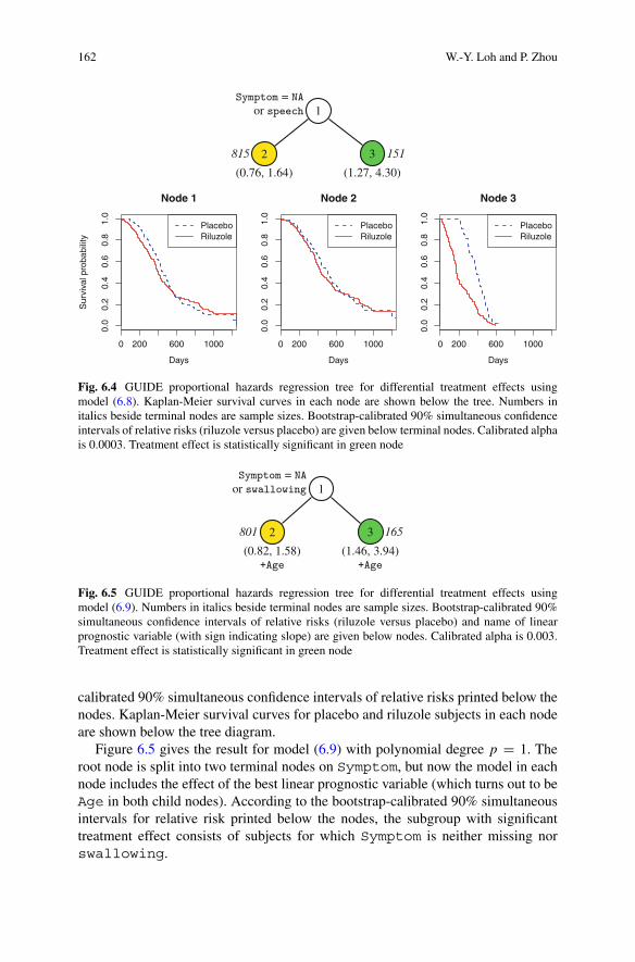
Figure 6.4 gives the result of fitting model (6.8) from the 966 subjects withnon-missing censored or observed survival time in the ALS data. The tree splitson Symptom to give two terminal nodes. The left node consists of 815 subjectswith Symptom either missing or is speech. The other 151 subjects go to the rightnode, which has a statistically significant treatment effect based on the bootstrap-


Symptom = NAor speech 1

815 2

(0.76, 1.64)

3

(1.27, 4.30)

151

0 200 600 1000

0.0

0.2

0.4

0.6

0.8

1.0

Days

Sur

viva

l pro

babi

lity

Node 1

PlaceboRiluzole

0 200 600 1000

0.0

0.2

0.4

0.6

0.8

1.0

Days

Node 2

PlaceboRiluzole

0 200 600 1000

0.0

0.2

0.4

0.6

0.8

1.0

Days

Node 3

PlaceboRiluzole

Fig. 6.4 GUIDE proportional hazards regression tree for differential treatment effects usingmodel (6.8). Kaplan-Meier survival curves in each node are shown below the tree. Numbers initalics beside terminal nodes are sample sizes. Bootstrap-calibrated 90% simultaneous confidenceintervals of relative risks (riluzole versus placebo) are given below terminal nodes. Calibrated alphais 0.0003. Treatment effect is statistically significant in green node

Symptom = NAor swallowing 1

801 2

(0.82, 1.58)+Age

3 165

(1.46, 3.94)+Age

Fig. 6.5 GUIDE proportional hazards regression tree for differential treatment effects usingmodel (6.9). Numbers in italics beside terminal nodes are sample sizes. Bootstrap-calibrated 90%simultaneous confidence intervals of relative risks (riluzole versus placebo) and name of linearprognostic variable (with sign indicating slope) are given below nodes. Calibrated alpha is 0.003.Treatment effect is statistically significant in green node

calibrated 90% simultaneous confidence intervals of relative risks printed below thenodes. Kaplan-Meier survival curves for placebo and riluzole subjects in each nodeare shown below the tree diagram.

Figure 6.5 gives the result for model (6.9) with polynomial degree p = 1. Theroot node is split into two terminal nodes on Symptom, but now the model in eachnode includes the effect of the best linear prognostic variable (which turns out to beAge in both child nodes). According to the bootstrap-calibrated 90% simultaneousintervals for relative risk printed below the nodes, the subgroup with significanttreatment effect consists of subjects for which Symptom is neither missing norswallowing.


6.6 Concluding Remarks

We have explained and demonstrated the main features of the GUIDE method forsubgroup identification and discussed a bootstrap method of confidence intervalconstruction for subgroup treatment effects. The bootstrap method is quite generaland is applicable to algorithms other than GUIDE. Because it expands the traditionalt-intervals to account for uncertainty due to split selection, it is more efficient ifthe estimated subgroup treatment effects are unbiased. The method may still beapplicable if the estimates are biased, but the calibrated intervals would be wideras a result. Biased estimates of subgroup treatment effects are common amongalgorithms that search for splits to maximize the difference in treatment effects inthe child nodes. A comparison of methods on this and other criteria is reported in aforthcoming article (Loh et al. 2019a).

Although GUIDE does not impute missing values for split selection, it doesimpute them in the predictor variables with their node sample means when fittingmodels (6.2)–(6.4) in the nodes. Therefore these models, e.g., Figs. 6.2 and 6.5,assume that missing values in the X variables are missing at random (MAR). Butthe MAR assumption is not needed for model (6.1), such as Figs. 6.1, 6.3, and 6.4.

There are two newer GUIDE features that are not discussed here. One is cyclic orperiodic predictor variables, such as angle of impact in an automobile crash, day ofweek of hospital admission, and time of day of medication administration. If GUIDEsplits a node on such a variable, the split takes the form of a finite interval of valuesa < X ≤ b instead of a half-line X ≤ c. Another feature is accommodation ofmultiple missing-value codes. For example, the result of a lab test may be “missing”for various reasons. It may not have been ordered by the physician because it wasrisky for the patient, it may be inappropriate (e.g., a mammogram for a male or aprostate-specific antigen test for a female), the patient may have declined the testdue to cost, or the result of the test was accidentally or erroneously not reported.If the “missing” values are all recorded as NA, a split would take the form “X ≤ c

or X = NA” or “X ≤ c and X �= NA”. But if the reasons for missingness areknown, GUIDE would use the information to produce more specific splits of theform “X ≤ c or X ∈ S”, where S is a subset of missing-value codes. Illustrativeexamples of these two features are given in the GUIDE manual (Loh 2018).

Acknowledgements The authors thank Tao Shen, Yu-Shan Shih and Shijie Tang for their helpfulcomments. Data used in the preparation of this article were obtained from the Pooled ResourceOpen-Access ALS Clinical Trials (PRO-ACT) Database. As such, the following organizations andindividuals within the PRO-ACT Consortium contributed to the design and implementation of thePRO-ACT Database and/or provided data, but did not participate in the analysis of the data or thewriting of this report: Neurological Clinical Research Institute, MGH Northeast ALS ConsortiumNovartis Prize4Life Israel Regeneron Pharmaceuticals, Inc., and Sanofi Teva PharmaceuticalIndustries, Ltd.


References

Aalen O (1978) Nonparametric inference for a family of counting processes. Ann Stat 6:701–726Ahn H, Loh W-Y (1994) Tree-structured proportional hazards regression modeling. Biometrics

50:471–485Aitkin M, Clayton D (1980) The fitting of exponential, Weibull and extreme value distributions to

complex censored survival data using GLIM. Appl Stat 29:156–163Atassi N, Berry J, Shui A, Zach N, Sherman A, Sinani E, Walker J, Katsovskiy I, Schoenfeld

D, Cudkowicz M, Leitner M (2014) The PRO-ACT database: Design, initial analyses, andpredictive features. Neurology 83(19):1719–1725

Breiman L, Friedman JH, Olshen RA, Stone CJ (1984) Classification and regression trees.Wadsworth, Belmont

Breslow N (1972) Contribution to the discussion of regression models and life tables by D. R. Cox.J R Stat Soc Ser B 34:216–217

Chan K-Y, Loh W-Y (2004) LOTUS: An algorithm for building accurate and comprehensiblelogistic regression trees. J. Comput. Graph. Stat. 13:826–852

Chaudhuri P, Loh W-Y (2002) Nonparametric estimation of conditional quantiles using quantileregression trees. Bernoulli 8:561–576

Chaudhuri P, Huang M-C, Loh W-Y, Yao R (1994) Piecewise-polynomial regression trees. Stat Sin4:143–167

Chaudhuri P, Lo W, Loh W, Yang C (1995) Generalized regression trees. Stat Sin 5:641–666Dusseldorp E, Meulman JJ (2004) The regression trunk approach to discover treatment covariate

interaction. Psychometrika 69:355–374Foster JC, Taylor JMG, Ruberg SJ (2011) Subgroup identification from randomized clinical trial

data. Stat Med 30:2867–2880Gnanadesikan R (1997) Methods for statistical data analysis of multivariate observations, 2nd edn.

Wiley, New YorkKim H, Loh W-Y (2001) Classification trees with unbiased multiway splits. J Am Stat Assoc

96:589–604Kim H, Loh W-Y (2003) Classification trees with bivariate linear discriminant node models. J

Comput Graph Stat 12:512–530Laird N, Olivier D (1981) Covariance analysis of censored survival data using log-linear analysis

techniques. J Am Stat Assoc 76:231–240Lawless J (1982) Statistical models and methods for lifetime data. Wiley, New YorkLipkovich I, Dmitrienko A (2014) Strategies for identifying predictive biomarkers and subgroups

with enhanced treatment effect in clinical trials using SIDES. J Biol Stand 24:130–153Lipkovich I, Dmitrienko A, Denne J, Enas G (2011) Subgroup identification based on differential

effect search — a recursive partitioning method for establishing response to treatment in patientsubpopulations. Stat Med 30:2601–2621

Loh W-Y (1987) Calibrating confidence coefficients. J Am Stat Assoc 82:155–162Loh W-Y (1991a) Bootstrap calibration for confidence interval construction and selection. Stat Sin

1:477–491Loh W-Y (1991b) Survival modeling through recursive stratification. Comput Stat Data Anal

12:295–313Loh W-Y (2002) Regression trees with unbiased variable selection and interaction detection. Stat

Sin 12:361–386Loh W-Y (2006) Regression tree models for designed experiments. In: Rojo J (ed) Second E. L.

Lehmann Symposium, vol 49. IMS lecture notes-monograph series. Institute of MathematicalStatistics, pp 210–228

Loh W-Y (2009) Improving the precision of classification trees. Ann Appl Stat 3:1710–1737Loh W-Y (2014) Fifty years of classification and regression trees (with discussion). Int Stat Rev

34:329–370Loh W-Y (2018) GUIDE user manual. University of Wisconsin, Madisons


Loh W-Y, Shih Y-S (1997) Split selection methods for classification trees. Stat Sin 7:815–840Loh W-Y, Vanichsetakul N (1988) Tree-structured classification via generalized discriminant

analysis (with discussion). J Am Stat Assoc 83:715–728Loh W-Y, Zheng W (2013) Regression trees for longitudinal and multiresponse data. Ann Appl

Stat 7:495–522Loh W-Y, He X, Man M (2015) A regression tree approach to identifying subgroups with

differential treatment effects. Stat Med 34:1818–1833Loh W-Y, Fu H, Man M, Champion V, Yu M (2016) Identification of subgroups with differential

treatment effects for longitudinal and multiresponse variables. Stat Med 35:4837–4855Loh W-Y, Cao L, Zhou P (2019a) Subgroup identification for precision medicine: a comparative

review of thirteen methods. Data Min Knowl Disc 9(5):e1326Loh W-Y, Eltinge J, Cho MJ, Li Y (2019b) Classification and regression trees and forests for

incomplete data from sample surveys. Stat Sin 29:431–453Loh W-Y, Man M, Wang S (2019c) Subgroups from regression trees with adjustment for prognostic

effects and post-selection inference. Stat Med 38:545–557Morgan JN, Sonquist JA (1963) Problems in the analysis of survey data, and a proposal. J Am Stat

Assoc 58:415–434Negassa A, Ciampi A, Abrahamowicz M, Shapiro S, Boivin J (2005) Tree-structured subgroup

analysis for censored survival data: validation of computationally inexpensive model selectioncriteria. Stat Comput 15:231–239

Seibold H, Zeileis A, Hothorn T (2016) Model-based recursive partitioning for subgroup analyses.Int J Biostat 12(1):45–63

Su X, Tsai C, Wang H, Nickerson D, Bogong L (2009) Subgroup analysis via recursivepartitioning. J Mach Learn Res 10:141–158

Therneau T, Atkinson B (2018) rpart: recursive partitioning and regression trees. R package version4.1-13

Zeileis A, Hothorn T, Hornik K (2008) Model-based recursive partitioning. J Comput Graph Stat17:492–514

chapter 6 the guide approach to subgroup identiﬁcation

Documents