chapter 7
DESCRIPTION
Chapter 7. Correlation, Bivariate Regression, and Multiple Regression. Pearson’s Product Moment Correlation. Correlation measures the association between two variables. Correlation quantifies the extent to which the mean, variation & direction of one variable are related to another variable. - PowerPoint PPT PresentationTRANSCRIPT

Chapter 7Chapter 7
Correlation, Bivariate Correlation, Bivariate Regression, and Multiple Regression, and Multiple RegressionRegression

Pearson’s Product Moment Pearson’s Product Moment CorrelationCorrelation
Correlation measures the association Correlation measures the association between two variables.between two variables.
Correlation quantifies the extent to Correlation quantifies the extent to which the mean, variation & direction which the mean, variation & direction of one variable are related to another of one variable are related to another variable.variable.
r ranges from +1 to -1.r ranges from +1 to -1. Correlation can be used for prediction.Correlation can be used for prediction. Correlation does not indicate the cause Correlation does not indicate the cause
of a relationship.of a relationship.
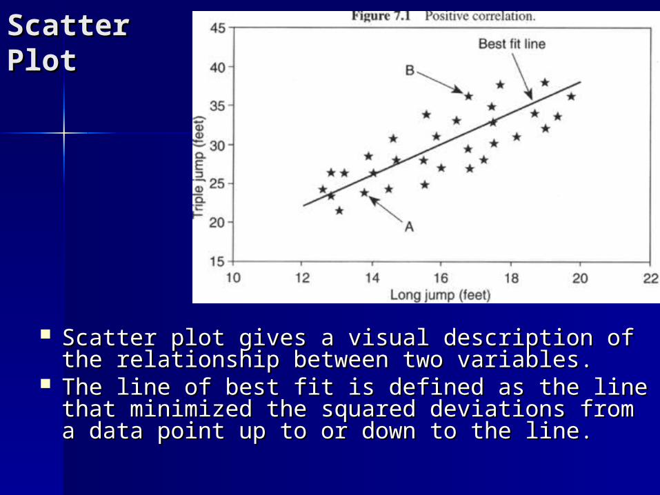
Scatter Scatter PlotPlot
Scatter plot gives a visual description of the Scatter plot gives a visual description of the relationship between two variables.relationship between two variables.
The line of best fit is defined as the line that The line of best fit is defined as the line that minimized the squared deviations from a minimized the squared deviations from a data point up to or down to the line.data point up to or down to the line.
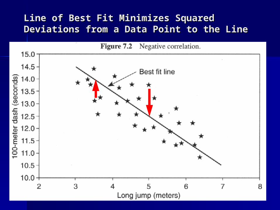
Line of Best Fit Minimizes Squared Line of Best Fit Minimizes Squared Deviations from a Data Point to the LineDeviations from a Data Point to the Line
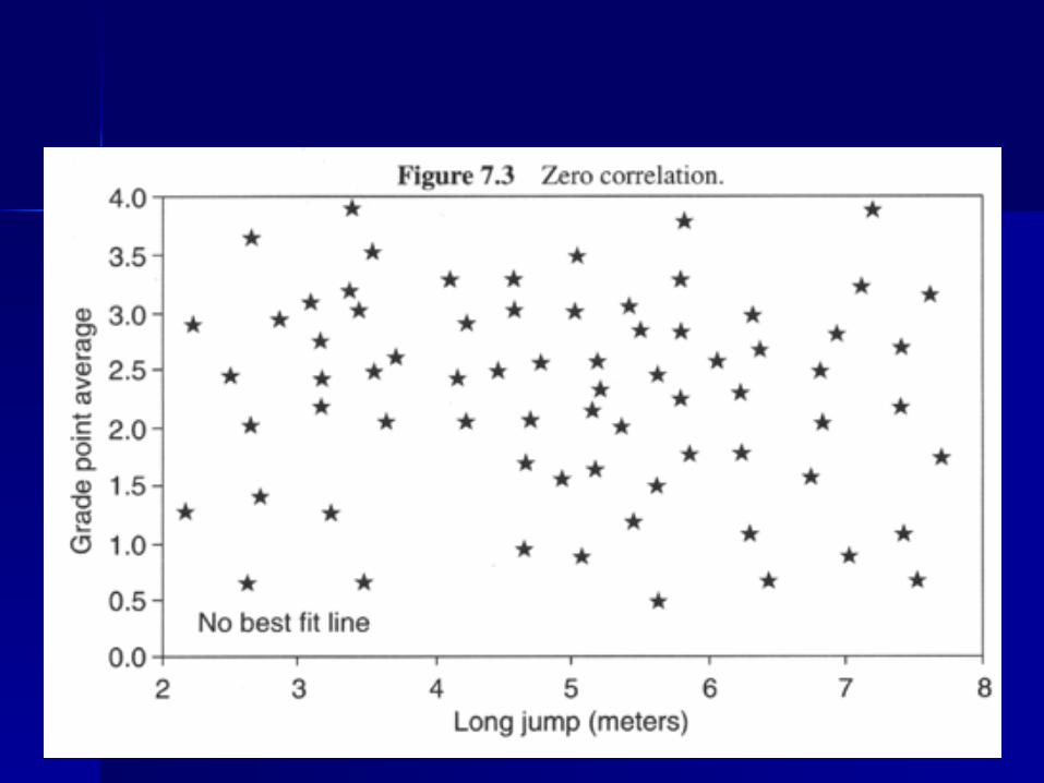

Always do a Scatter Plot to Check the Always do a Scatter Plot to Check the Shape of the RelationshipShape of the Relationship
-4
-3
-2
-1
0
1
2
0 1 2 3 4 5 6
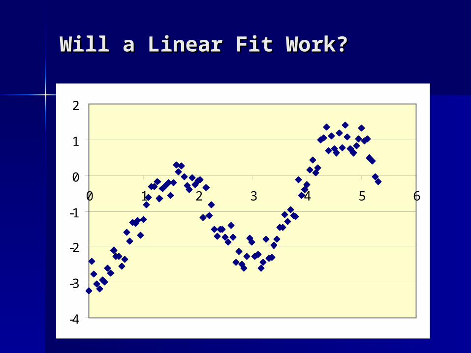
Will a Linear Fit Work?Will a Linear Fit Work?
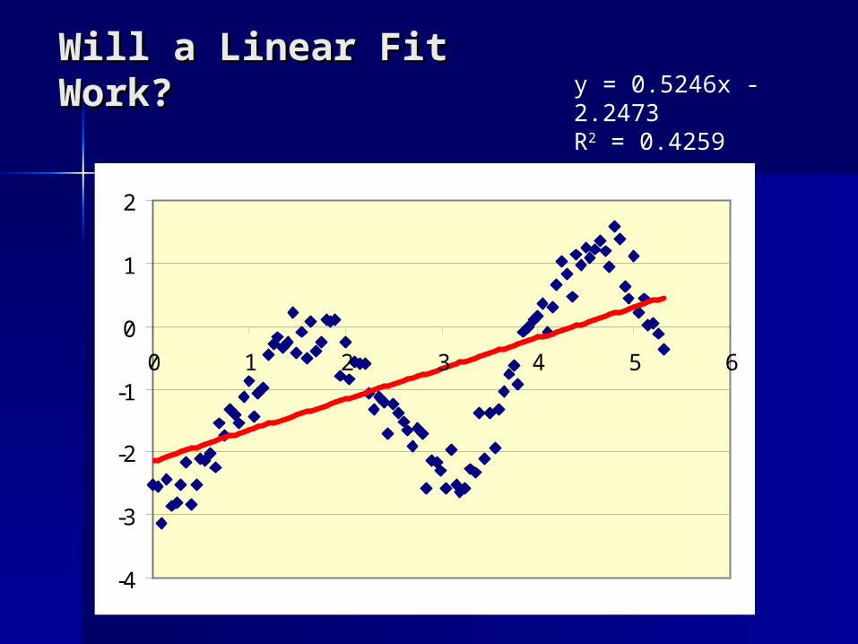
Will a Linear Fit Will a Linear Fit Work?Work? y = 0.5246x -
2.2473R2 = 0.4259
-4
-3
-2
-1
0
1
2
0 1 2 3 4 5 6

22ndnd Order Order Fit?Fit? y = 0.0844x2 + 0.1057x -
1.9492R2 = 0.4666
-4
-3
-2
-1
0
1
2
0 1 2 3 4 5 6

66thth Order Order Fit?Fit?
y = 0.0341x6 - 0.6358x5 + 4.3835x4 - 13.609x3 + 18.224x2 - 7.3526x - 2.0039R2 = 0.9337
-4
-3
-2
-1
0
1
2
0 1 2 3 4 5 6

Will Linear Fit Will Linear Fit Work?Work?
Y
-4
-3
-2
-1
0
1
2
0 50 100 150 200 250
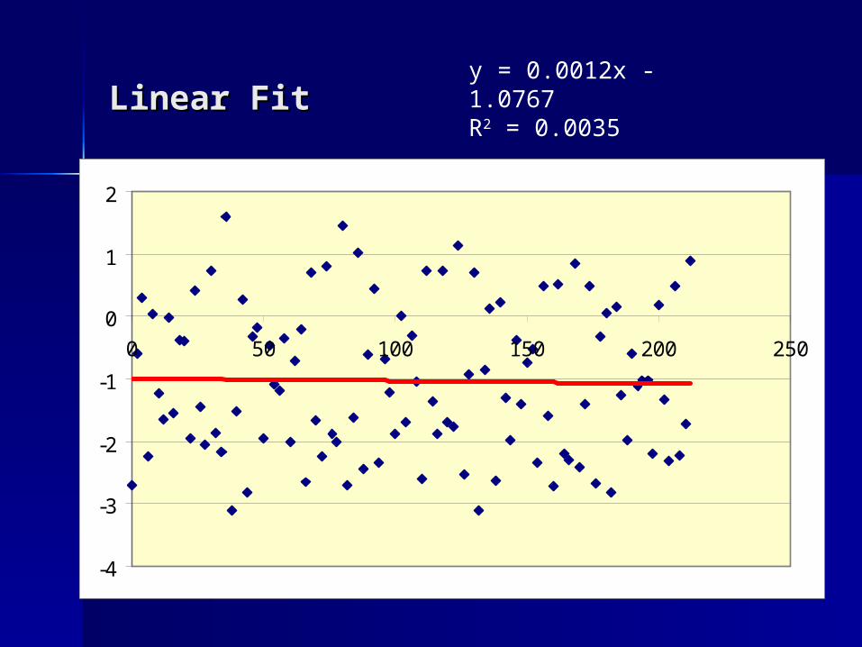
Linear FitLinear Fity = 0.0012x - 1.0767R2 = 0.0035
-4
-3
-2
-1
0
1
2
0 50 100 150 200 250


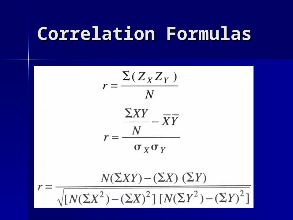
Correlation FormulasCorrelation Formulas

Evaluating the Strength of a Evaluating the Strength of a CorrelationCorrelation For predictions, absolute value of r < .7, For predictions, absolute value of r < .7,
may produce unacceptably large errors, may produce unacceptably large errors, especially if the SDs of either or both X & especially if the SDs of either or both X & Y are large.Y are large.
As a general rule As a general rule – Absolute value r greater than or equal .9 is Absolute value r greater than or equal .9 is
goodgood– Absolute value r equal to .7 - .8 is moderateAbsolute value r equal to .7 - .8 is moderate– Absolute value r equal to .5 - .7 is lowAbsolute value r equal to .5 - .7 is low– Values for r below .5 give RValues for r below .5 give R22 = .25, or 25% are = .25, or 25% are
poor, and thus not useful for predicting.poor, and thus not useful for predicting.
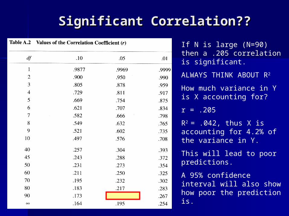
Significant Correlation??Significant Correlation??
If N is large (N=90) then a .205 correlation is significant.
ALWAYS THINK ABOUT R2
How much variance in Y is X accounting for?
r = .205
R2 = .042, thus X is accounting for 4.2% of the variance in Y.
This will lead to poor predictions.
A 95% confidence interval will also show how poor the prediction is.
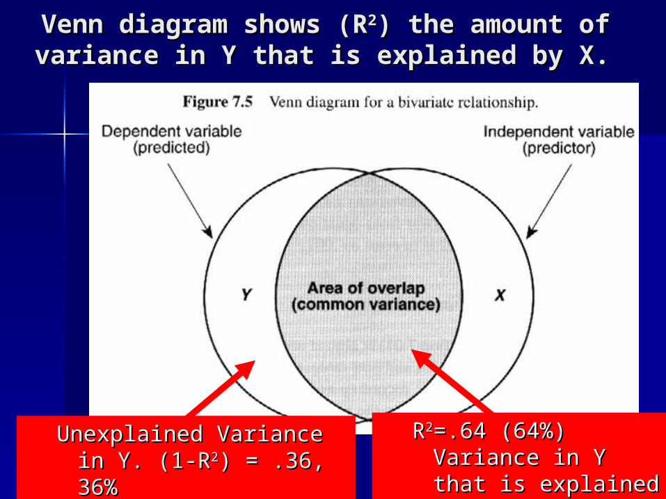
Venn diagram shows (RVenn diagram shows (R22) the amount ) the amount of variance in Y that is explained by X.of variance in Y that is explained by X.
Unexplained Variance in Unexplained Variance in Y. (1-RY. (1-R22) = .36, 36%) = .36, 36%
RR22=.64 (64%) =.64 (64%) Variance in Y that is Variance in Y that is explained by Xexplained by X

The vertical The vertical distance (up distance (up or down) or down) from a data from a data point to the point to the line of best line of best fit is a fit is a RESIDUAL.RESIDUAL.
r = .845r = .845
RR22 = .714 = .714 (71.4%)(71.4%)
Y = mX + bY = mX + b
Y = .72 X + Y = .72 X + 1313

– If r < .7 If r < .7 prediction prediction will be will be poor.poor.
– Large SDs Large SDs adversely adversely affect the affect the accuracy accuracy of the of the prediction.prediction.
Calculation of Regression Coefficients Calculation of Regression Coefficients (b, C)(b, C)

Standard Deviation of Standard Deviation of ResidualsResiduals

– The SEThe SEEE is the SD of the prediction errors is the SD of the prediction errors (residuals) when predicting Y from X. SE(residuals) when predicting Y from X. SEEE is used is used to make a confidence interval for the prediction to make a confidence interval for the prediction equation.equation.
Standard Error of Standard Error of EstimateEstimate(SE(SEEE))
SD of YSD of Y
Prediction Prediction ErrorsErrors

The SEThe SEEE is used to compute confidence is used to compute confidence intervals for prediction equation.intervals for prediction equation.

Example of a 95% confidence Example of a 95% confidence interval.interval.
– Both r and SDY are critical in accuracy of prediction.
– If SDIf SDYY is small and r is big, is small and r is big, predictions are will be small.predictions are will be small.
– If SDIf SDYY is big and r is small, is big and r is small, predictions are will be large.predictions are will be large.
– We are 95% We are 95% sure the sure the mean falls mean falls between 45.1 between 45.1 and 67.3and 67.3

Multiple RegressionMultiple Regression
Multiple regression is used to predict Multiple regression is used to predict one Y (dependent) variable from two one Y (dependent) variable from two or more X (independent) variables.or more X (independent) variables.
The advantage of multivariate or The advantage of multivariate or bivariate regression isbivariate regression is– Provides lower standard error of Provides lower standard error of
estimateestimate– Determines which variables contribute Determines which variables contribute
to the prediction and which do not.to the prediction and which do not.
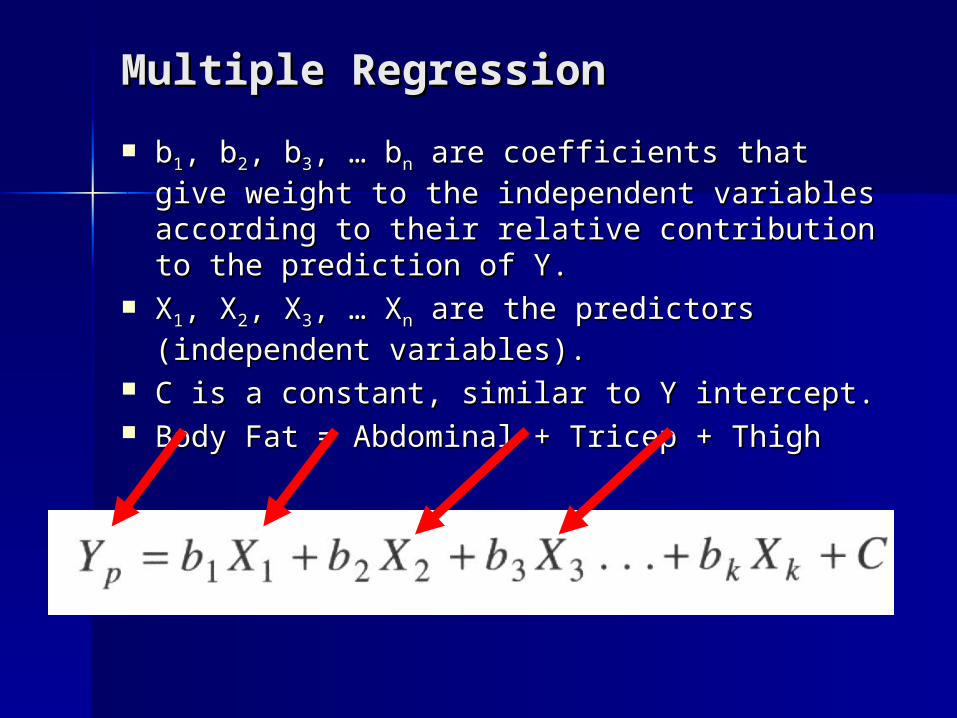
Multiple RegressionMultiple Regression
bb11, b, b22, b, b33, … b, … bnn are coefficients that give are coefficients that give weight to the independent variables weight to the independent variables according to their relative contribution to the according to their relative contribution to the prediction of Y.prediction of Y.
XX11, X, X22, X, X33, … X, … Xnn are the predictors are the predictors (independent variables).(independent variables).
C is a constant, similar to Y intercept.C is a constant, similar to Y intercept. Body Fat = Abdominal + Tricep + ThighBody Fat = Abdominal + Tricep + Thigh

List the variables and order to enter into List the variables and order to enter into the equationthe equation
1.1. XX22 has biggest has biggest area (C), it comes area (C), it comes in first.in first.
2.2. XX11 comes in next comes in next area (A) is bigger area (A) is bigger than area (E). than area (E). Both A and E are Both A and E are unique, not unique, not common to C.common to C.
3.3. XX33 comes in next, comes in next, it uniquely adds it uniquely adds area (E).area (E).
4.4. XX44 is not related is not related to Y so it is NOT to Y so it is NOT in the equation.in the equation.

Ideal Relationship Between Predictors and Ideal Relationship Between Predictors and YY
– Each variable Each variable accounts for accounts for unique unique variance in Yvariance in Y
– Very little Very little overlap of the overlap of the predictorspredictors
– Order to enter?Order to enter?
– XX11, X, X33, X, X44, X, X22, , XX55


Regression MethodsRegression Methods
Enter: forces all predictors (independent Enter: forces all predictors (independent variables) into the equation, in one step.variables) into the equation, in one step.
Forward: Each step adds a new predictor. Forward: Each step adds a new predictor. Predictors enter based upon the unique Predictors enter based upon the unique variance in Y they explain.variance in Y they explain.
Backward: Starts with full equation (all Backward: Starts with full equation (all predictors) and removes them one at a predictors) and removes them one at a time on each step, beginning with the time on each step, beginning with the predictor that adds the least.predictor that adds the least.
Stepwise: Each step adds a new Stepwise: Each step adds a new predictor. One any step a predictor can predictor. One any step a predictor can be added and another removed if it has be added and another removed if it has high partial correlations with the newly high partial correlations with the newly added predictor.added predictor.
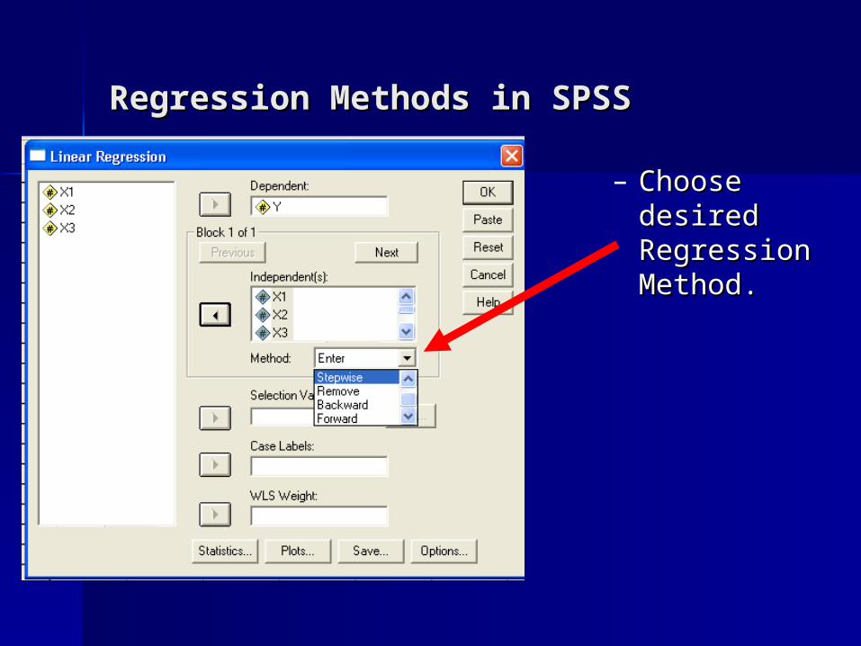
Regression Methods in SPSSRegression Methods in SPSS
– Choose Choose desired desired Regression Regression Method.Method.
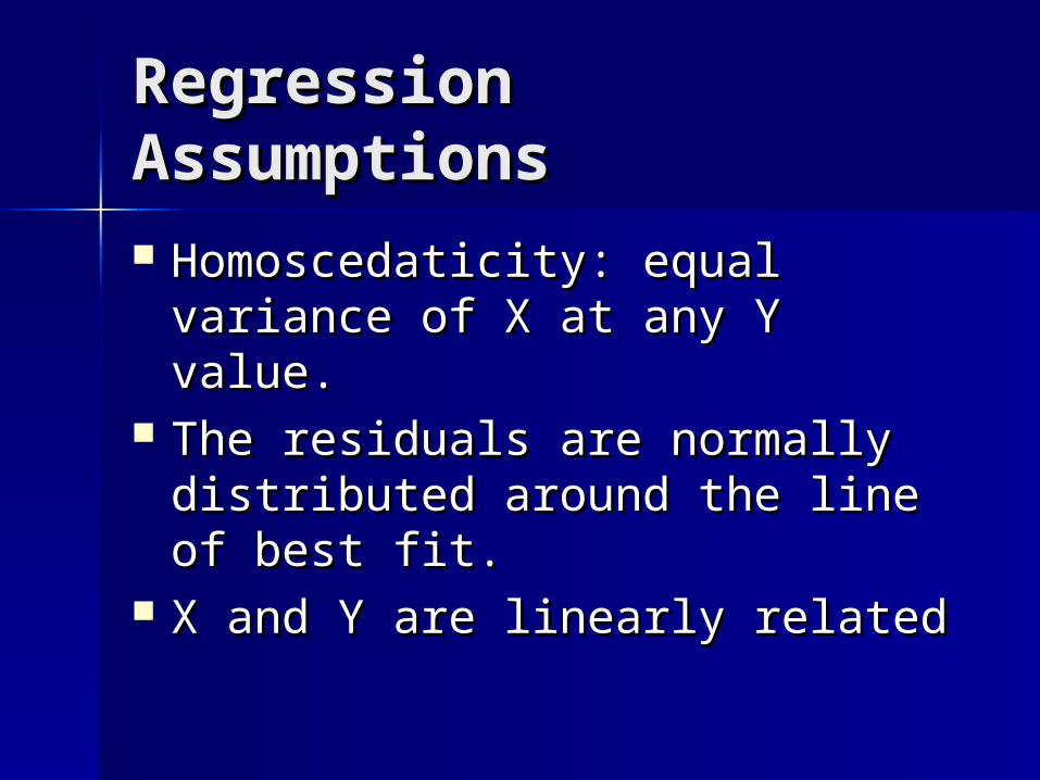
Regression Regression AssumptionsAssumptions Homoscedaticity: equal variance Homoscedaticity: equal variance
of X at any Y value.of X at any Y value. The residuals are normally The residuals are normally
distributed around the line of best distributed around the line of best fit.fit.
X and Y are linearly relatedX and Y are linearly related

Tests for Tests for NormalitNormality y
Set 1 Set 2 Set 3 Set 4
11 123 2 5
25 144 5 29
14 155 4 24
17 144 7 25
14 125 1 31
10 147 9 37
9 182 5 35
22 166 6 22
25 122 8 24
27 165 7 25
24 143 9 30
11 156 4 28
19 154 2 25
25 149 22 26
– Use SPSSUse SPSS
– DescriptivesDescriptives
–ExploreExplore

Tests for Normality Tests for Normality

Tests for Normality Tests for Normality

Tests for Normality Tests for Normality
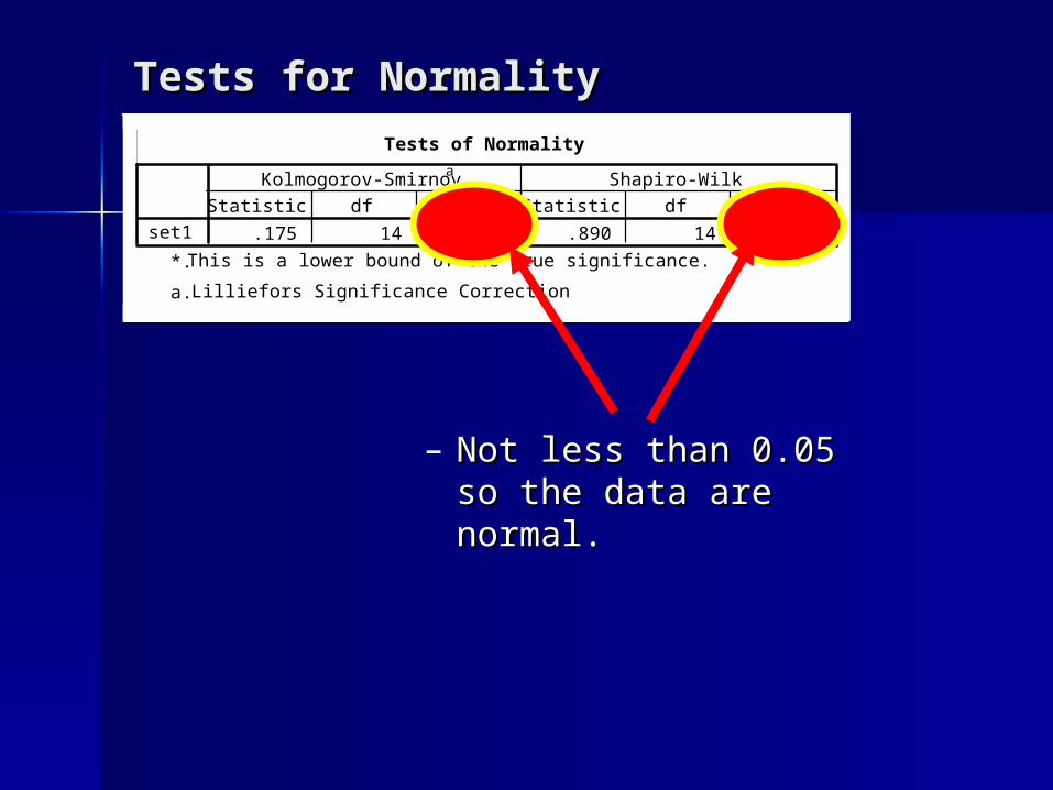
Tests for Normality Tests for Normality Tests of Normality
.175 14 .200* .890 14 .081set1Statistic df Sig. Statistic df Sig.
Kolmogorov-Smirnova
Shapiro-Wilk
This is a lower bound of the true significance.*.
Lilliefors Significance Correctiona.
– Not less than 0.05 so Not less than 0.05 so the data are normal.the data are normal.
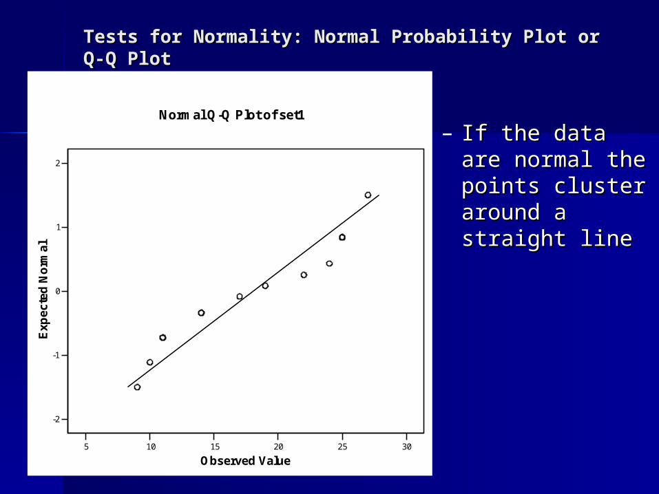
Tests for Normality: Normal Probability Plot or Q-Q Tests for Normality: Normal Probability Plot or Q-Q PlotPlot
5 10 15 20 25 30
Observed Value
-2
-1
0
1
2
Exp
ecte
d N
orm
al
Normal Q-Q Plot of set1
– If the data are If the data are normal the normal the points cluster points cluster around a straight around a straight lineline

Tests for Normality: Tests for Normality: BoxplotsBoxplots
set1
9.00
12.00
15.00
18.00
21.00
24.00
27.00
– Bar is the median, box Bar is the median, box extends from 25 – 75extends from 25 – 75thth percentile, whiskers extend to percentile, whiskers extend to largest and smallest values largest and smallest values within 1.5 box lengthswithin 1.5 box lengths
set1
0.00
20.00
40.00
60.00
80.00
100.00
16
15
– Outliers are labeled Outliers are labeled with O, Extreme with O, Extreme values are labeled with values are labeled with a stara star

Tests for Normality: Normal Probability Tests for Normality: Normal Probability Plot or Q-Q PlotPlot or Q-Q Plot
5 10 15 20 25 30
Observed Value
-2
-1
0
1
2
Exp
ecte
d N
orm
al
Normal Q-Q Plot of set1
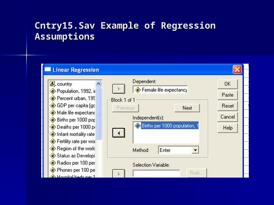
Cntry15.Sav Example of Regression Cntry15.Sav Example of Regression AssumptionsAssumptions

Cntry15.Sav Example of Regression Cntry15.Sav Example of Regression AssumptionsAssumptions
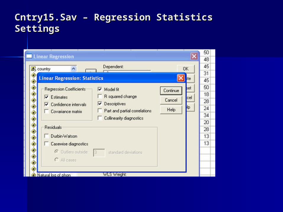
Cntry15.Sav – Regression Statistics SettingsCntry15.Sav – Regression Statistics Settings
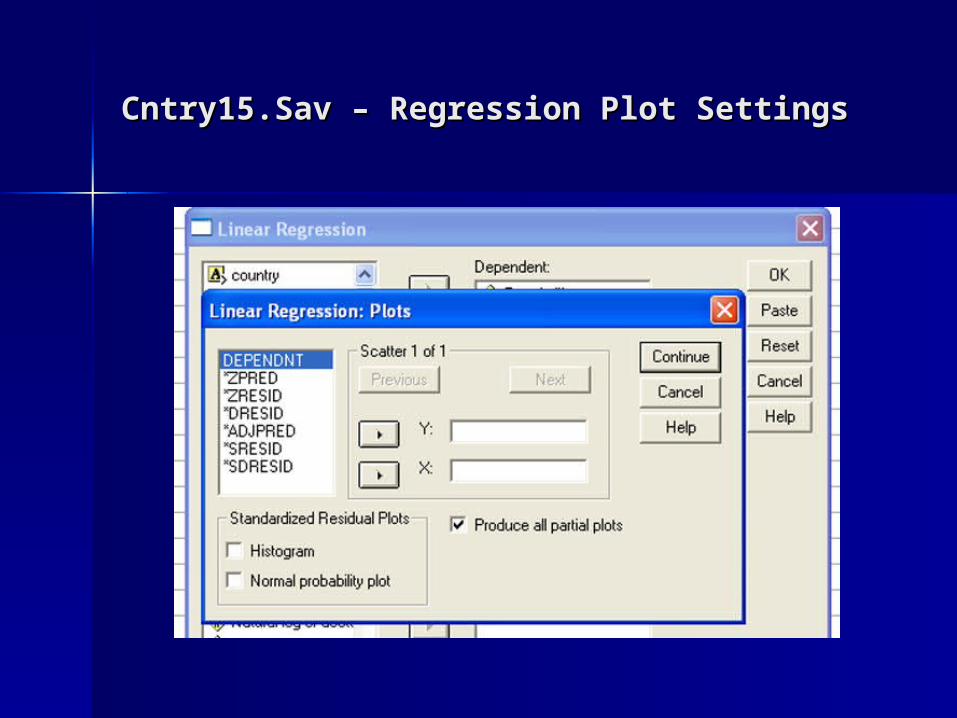
Cntry15.Sav – Regression Plot SettingsCntry15.Sav – Regression Plot Settings
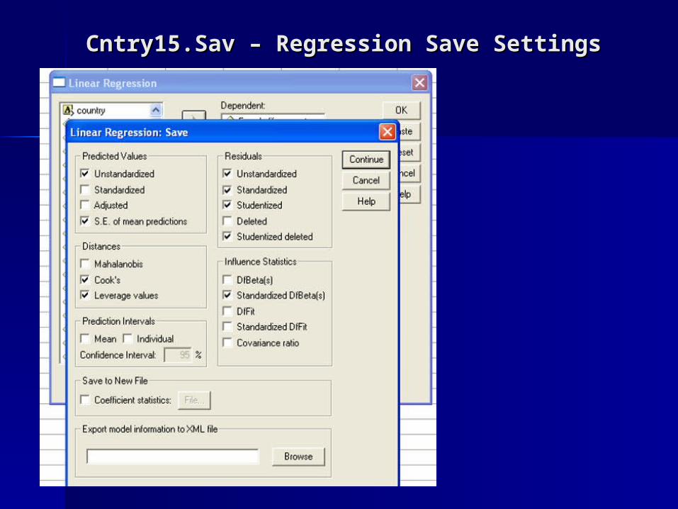
Cntry15.Sav – Regression Save SettingsCntry15.Sav – Regression Save Settings
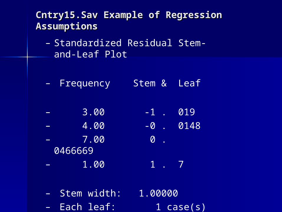
Cntry15.Sav Example of Regression Cntry15.Sav Example of Regression AssumptionsAssumptions
– Standardized Residual Stem-and-Leaf Plot
– Frequency Stem & Leaf
– 3.00 -1 . 019– 4.00 -0 . 0148– 7.00 0 . 0466669– 1.00 1 . 7
– Stem width: 1.00000– Each leaf: 1 case(s)

Cntry15.Sav Example of Regression Cntry15.Sav Example of Regression AssumptionsAssumptions
-2 -1 0 1 2
Observed Value
-2
-1
0
1
2
Exp
ecte
d N
orm
al
Normal Q-Q Plot of Standardized Residual
– Distribution Distribution is normal.is normal.
– Two scores Two scores are are somewhat somewhat outsideoutside

Cntry15.Sav Example of Regression Cntry15.Sav Example of Regression AssumptionsAssumptions
Standardized Residual
-2.00000
-1.00000
0.00000
1.00000
2.00000
– No Outliers No Outliers [labeled O] [labeled O]
– No Extreme No Extreme scores scores [labeled with [labeled with a star]a star]

Cntry15.Sav Example of Regression AssumptionsCntry15.Sav Example of Regression Assumptions
-2 -1 0 1 2
Observed Value
-0.6
-0.4
-0.2
0.0
0.2
0.4
Dev
fro
m N
orm
al
Detrended Normal Q-Q Plot of Standardized Residual– The points The points
should fall should fall randomly in randomly in a band a band around 0, if around 0, if the the distribution distribution is normal.is normal.
– In this In this distribution distribution there is one there is one extreme extreme score.score.

Cntry15.Sav Example of Regression Cntry15.Sav Example of Regression AssumptionsAssumptions
Extreme Values
6 1.73204
3 .97994
11 .67940
8 .61749
9 .60691a
12 -1.98616
1 -1.14647
4 -1.02716
7 -.83536
10 -.49254
1
2
3
4
5
1
2
3
4
5
Highest
Lowest
Standardized ResidualCase Number Value
Only a partial list of cases with the value .60691 are shown in thetable of upper extremes.
a.
Tests of Normality
.137 15 .200* .971 15 .866Standardized ResidualStatistic df Sig. Statistic df Sig.
Kolmogorov-Smirnova
Shapiro-Wilk
This is a lower bound of the true significance.*.
Lilliefors Significance Correctiona.
– The data are The data are normal.normal.

Regression ViolationsRegression Violations
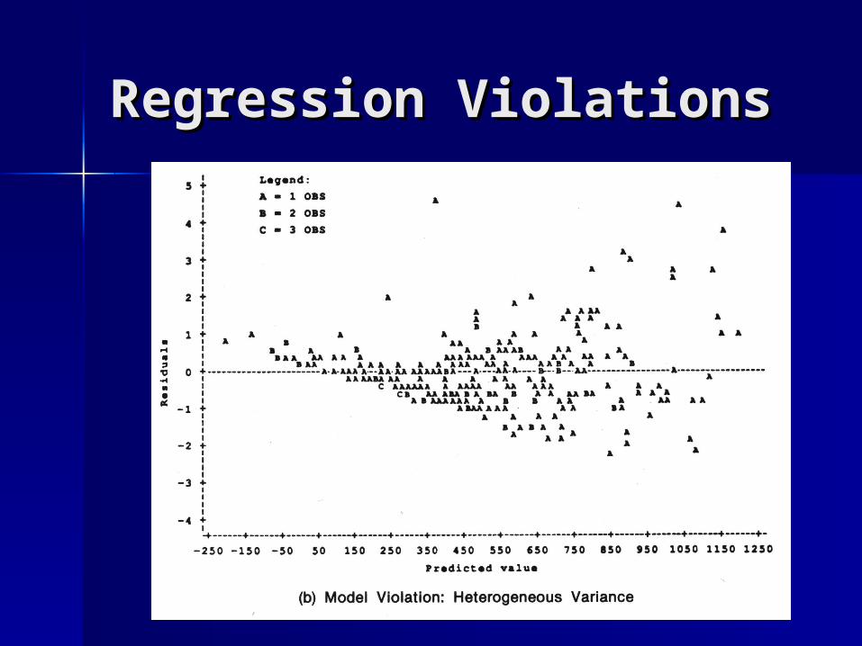
Regression ViolationsRegression Violations

Regression ViolationsRegression Violations