chapter 7
DESCRIPTION
Chapter 7. Hypothesis Testing with One Sample. Chapter Outline. 7.1 Introduction to Hypothesis Testing 7.2 Hypothesis Testing for the Mean (Large Samples) 7.3 Hypothesis Testing for the Mean (Small Samples) 7.4 Hypothesis Testing for Proportions - PowerPoint PPT PresentationTRANSCRIPT

Chapter 7
Hypothesis Testing with One Sample
1Larson/Farber 4th ed.

Chapter Outline
• 7.1 Introduction to Hypothesis Testing
• 7.2 Hypothesis Testing for the Mean (Large Samples)
• 7.3 Hypothesis Testing for the Mean (Small Samples)
• 7.4 Hypothesis Testing for Proportions
• 7.5 Hypothesis Testing for Variance and Standard Deviation
2Larson/Farber 4th ed.

Section 7.1
Introduction to Hypothesis Testing
3Larson/Farber 4th ed.

Section 7.1 Objectives
• State a null hypothesis and an alternative hypothesis
• Identify type I and type I errors and interpret the level of significance
• Determine whether to use a one-tailed or two-tailed statistical test and find a p-value
• Make and interpret a decision based on the results of a statistical test
• Write a claim for a hypothesis test
4Larson/Farber 4th ed.

Hypothesis Tests
Hypothesis test
• A process that uses sample statistics to test a claim about the value of a population parameter.
• For example: An automobile manufacturer advertises that its new hybrid car has a mean mileage of 50 miles per gallon. To test this claim, a sample would be taken. If the sample mean differs enough from the advertised mean, you can decide the advertisement is wrong.
5Larson/Farber 4th ed.

Hypothesis Tests
Statistical hypothesis
• A statement, or claim, about a population parameter.
• Need a pair of hypotheses
• one that represents the claim
• the other, its complement
• When one of these hypotheses is false, the other must be true.
6Larson/Farber 4th ed.

Stating a Hypothesis
Null hypothesis
• A statistical hypothesis that contains a statement of equality such as , =, or .
• Denoted H0 read “H subzero” or “H naught.”
Alternative hypothesis
• A statement of inequality such as >, , or <.
• Must be true if H0 is false.
• Denoted Ha read “H sub-a.”
complementary statements
7Larson/Farber 4th ed.

Stating a Hypothesis
• To write the null and alternative hypotheses, translate the claim made about the population parameter from a verbal statement to a mathematical statement.
• Then write its complement.
H0: μ ≤ kHa: μ > k
H0: μ ≥ kHa: μ < k
H0: μ = kHa: μ ≠ k
• Regardless of which pair of hypotheses you use, you always assume μ = k and examine the sampling distribution on the basis of this assumption.
8Larson/Farber 4th ed.

Example: Stating the Null and Alternative Hypotheses
Write the claim as a mathematical sentence. State the null and alternative hypotheses and identify which represents the claim.1.A university publicizes that the proportion of its students who graduate in 4 years is 82%.
Equality condition
Complement of H0
H0:
Ha:
(Claim)p = 0.82
p ≠ 0.82
Solution:
9Larson/Farber 4th ed.

μ ≥ 2.5 gallons per minute
Example: Stating the Null and Alternative Hypotheses
Write the claim as a mathematical sentence. State the null and alternative hypotheses and identify which represents the claim.2.A water faucet manufacturer announces that the mean flow rate of a certain type of faucet is less than 2.5 gallons per minute.
Inequality condition
Complement of HaH0:
Ha:(Claim)μ < 2.5 gallons per minute
Solution:
10Larson/Farber 4th ed.

μ ≤ 20 ounces
Example: Stating the Null and Alternative Hypotheses
Write the claim as a mathematical sentence. State the null and alternative hypotheses and identify which represents the claim.3.A cereal company advertises that the mean weight of the contents of its 20-ounce size cereal boxes is more than 20 ounces.
Inequality condition
Complement of HaH0:
Ha:(Claim)μ > 20 ounces
Solution:
11Larson/Farber 4th ed.

Types of Errors
• No matter which hypothesis represents the claim, always begin the hypothesis test assuming that the equality condition in the null hypothesis is true.
• At the end of the test, one of two decisions will be made: reject the null hypothesis fail to reject the null hypothesis
• Because your decision is based on a sample, there is the possibility of making the wrong decision.
12Larson/Farber 4th ed.

Types of Errors
• A type I error occurs if the null hypothesis is rejected when it is true.
• A type II error occurs if the null hypothesis is not rejected when it is false.
Actual Truth of H0
Decision H0 is true H0 is false
Do not reject H0 Correct Decision Type II Error
Reject H0 Type I Error Correct Decision
13Larson/Farber 4th ed.

Example: Identifying Type I and Type II Errors
The USDA limit for salmonella contamination for chicken is 20%. A meat inspector reports that the chicken produced by a company exceeds the USDA limit. You perform a hypothesis test to determine whether the meat inspector’s claim is true. When will a type I or type II error occur? Which is more serious? (Source: United States Department of Agriculture)
14Larson/Farber 4th ed.

Let p represent the proportion of chicken that is contaminated.
Solution: Identifying Type I and Type II Errors
H0:
Ha:
p ≤ 0.2
p > 0.2
Hypotheses:
(Claim)
0.16 0.18 0.20 0.22 0.24p
H0: p ≤ 0.20 H0: p > 0.20
Chicken meets USDA limits.
Chicken exceeds USDA limits.
15Larson/Farber 4th ed.

Solution: Identifying Type I and Type II Errors
A type I error is rejecting H0 when it is true.
The actual proportion of contaminated chicken is lessthan or equal to 0.2, but you decide to reject H0.
A type II error is failing to reject H0 when it is false.
The actual proportion of contaminated chicken is greater than 0.2, but you do not reject H0.
H0:Ha:
p ≤ 0.2p > 0.2
Hypotheses:(Claim)
16Larson/Farber 4th ed.

Solution: Identifying Type I and Type II Errors
H0:Ha:
p ≤ 0.2p > 0.2
Hypotheses:(Claim)
• With a type I error, you might create a health scare and hurt the sales of chicken producers who were actually meeting the USDA limits.
• With a type II error, you could be allowing chicken that exceeded the USDA contamination limit to be sold to consumers.
• A type II error could result in sickness or even death.
17Larson/Farber 4th ed.

Level of Significance
Level of significance • Your maximum allowable probability of making a
type I error. Denoted by , the lowercase Greek letter alpha.
• By setting the level of significance at a small value, you are saying that you want the probability of rejecting a true null hypothesis to be small.
• Commonly used levels of significance: = 0.10 = 0.05 = 0.01
• P(type II error) = β (beta)
18Larson/Farber 4th ed.

Statistical Tests
• After stating the null and alternative hypotheses and specifying the level of significance, a random sample is taken from the population and sample statistics are calculated.
• The statistic that is compared with the parameter in the null hypothesis is called the test statistic.
σ2
x
χ2 (Section 7.5)s2
z (Section 7.4)pt (Section 7.3 n < 30)z (Section 7.2 n 30)μ
Standardized test statistic
Test statisticPopulation parameter
p̂
19Larson/Farber 4th ed.

P-values
P-value (or probability value)
• The probability, if the null hypothesis is true, of obtaining a sample statistic with a value as extreme or more extreme than the one determined from the sample data.
• Depends on the nature of the test.
20Larson/Farber 4th ed.

Nature of the Test
• Three types of hypothesis tests left-tailed test right-tailed test two-tailed test
• The type of test depends on the region of the sampling distribution that favors a rejection of H0.
• This region is indicated by the alternative hypothesis.
21Larson/Farber 4th ed.

Left-tailed Test
• The alternative hypothesis Ha contains the less-than inequality symbol (<).
z
0 1 2 3-3 -2 -1
Test statistic
H0: μ k
Ha: μ < k
P is the area to the left of the test statistic.
22Larson/Farber 4th ed.

• The alternative hypothesis Ha contains the greater-than inequality symbol (>).
z
0 1 2 3-3 -2 -1
Right-tailed Test
H0: μ ≤ k
Ha: μ > k
Test statistic
P is the area to the right of the test statistic.
23Larson/Farber 4th ed.

Two-tailed Test
• The alternative hypothesis Ha contains the not equal inequality symbol (≠). Each tail has an area of ½P.
z
0 1 2 3-3 -2 -1
Test statistic
Test statistic
H0: μ = k
Ha: μ kP is twice the area to the left of the negative test statistic.
P is twice the area to the right of the positive test statistic.
24Larson/Farber 4th ed.

Example: Identifying The Nature of a Test
For each claim, state H0 and Ha. Then determine whether the hypothesis test is a left-tailed, right-tailed, or two-tailed test. Sketch a normal sampling distribution and shade the area for the P-value.1.A university publicizes that the proportion of its students who graduate in 4 years is 82%.
H0:Ha:
p = 0.82p ≠ 0.82
Two-tailed testz
0-z z
½ P-value area
½ P-value area
Solution:
25Larson/Farber 4th ed.

Example: Identifying The Nature of a Test
For each claim, state H0 and Ha. Then determine whether the hypothesis test is a left-tailed, right-tailed, or two-tailed test. Sketch a normal sampling distribution and shade the area for the P-value.2.A water faucet manufacturer announces that the mean flow rate of a certain type of faucet is less than 2.5 gallons per minute.
H0:Ha:
Left-tailed testz
0-z
P-value area
μ ≥ 2.5 gpmμ < 2.5 gpm
Solution:
26Larson/Farber 4th ed.

Example: Identifying The Nature of a Test
For each claim, state H0 and Ha. Then determine whether the hypothesis test is a left-tailed, right-tailed, or two-tailed test. Sketch a normal sampling distribution and shade the area for the P-value.3.A cereal company advertises that the mean weight of the contents of its 20-ounce size cereal boxes is more than 20 ounces.
H0:Ha:
Right-tailed testz
0 z
P-value areaμ ≤ 20 oz
μ > 20 oz
Solution:
27Larson/Farber 4th ed.

Making a Decision
Decision Rule Based on P-value• Compare the P-value with .
If P , then reject H0.
If P > , then fail to reject H0.
Claim
Decision Claim is H0 Claim is Ha
Fail to reject H0
Reject H0
There is enough evidence to reject the claim
There is not enough evidence to reject the claim
There is enough evidence to support the claim
There is not enough evidence to support the claim
28Larson/Farber 4th ed.

Example: Interpreting a Decision
You perform a hypothesis test for the following claim. How should you interpret your decision if you reject H0? If you fail to reject H0?
1.H0 (Claim): A university publicizes that the proportion of its students who graduate in 4 years is 82%.
29Larson/Farber 4th ed.

Solution: Interpreting a Decision
• The claim is represented by H0.
• If you reject H0 you should conclude “there is sufficient evidence to indicate that the university’s claim is false.”
• If you fail to reject H0, you should conclude “there is insufficient evidence to indicate that the university’s claim (of a four-year graduation rate of 82%) is false.”
30Larson/Farber 4th ed.

Example: Interpreting a Decision
You perform a hypothesis test for the following claim. How should you interpret your decision if you reject H0? If you fail to reject H0?
2.Ha (Claim): Consumer Reports states that the mean stopping distance (on a dry surface) for a Honda Civic is less than 136 feet.Solution:
• The claim is represented by Ha.
• H0 is “the mean stopping distance…is greater than or equal to 136 feet.”
31Larson/Farber 4th ed.

Solution: Interpreting a Decision
• If you reject H0 you should conclude “there is enough evidence to support Consumer Reports’ claim that the stopping distance for a Honda Civic is less than 136 feet.”
• If you fail to reject H0, you should conclude “there is not enough evidence to support Consumer Reports’ claim that the stopping distance for a Honda Civic is less than 136 feet.”
32Larson/Farber 4th ed.

z0
Steps for Hypothesis Testing
1. State the claim mathematically and verbally. Identify the null and alternative hypotheses.
H0: ? Ha: ?2. Specify the level of significance.
α = ?3. Determine the standardized
sampling distribution and draw its graph.
4. Calculate the test statisticand its standardized value.Add it to your sketch. z
0Test statistic
This sampling distribution is based on the assumption that H0 is true.
33Larson/Farber 4th ed.
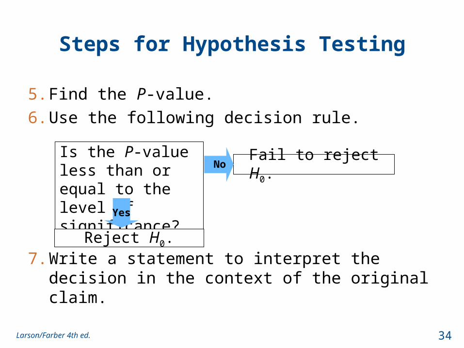
Steps for Hypothesis Testing
5. Find the P-value.
6. Use the following decision rule.
7. Write a statement to interpret the decision in the context of the original claim.
Is the P-value less than or equal to the level of significance?
Fail to reject H0.
Yes
Reject H0.
No
34Larson/Farber 4th ed.

Section 7.1 Summary
• Stated a null hypothesis and an alternative hypothesis
• Identified type I and type I errors and interpreted the level of significance
• Determined whether to use a one-tailed or two-tailed statistical test and found a p-value
• Made and interpreted a decision based on the results of a statistical test
• Wrote a claim for a hypothesis test
35Larson/Farber 4th ed.

Section 7.2
Hypothesis Testing for the Mean (Large Samples)
36Larson/Farber 4th ed.

Section 7.2 Objectives
• Find P-values and use them to test a mean μ
• Use P-values for a z-test
• Find critical values and rejection regions in a normal distribution
• Use rejection regions for a z-test
37Larson/Farber 4th ed.

Using P-values to Make a Decision
Decision Rule Based on P-value
• To use a P-value to make a conclusion in a hypothesis test, compare the P-value with .
1. If P , then reject H0.
2. If P > , then fail to reject H0.
38Larson/Farber 4th ed.
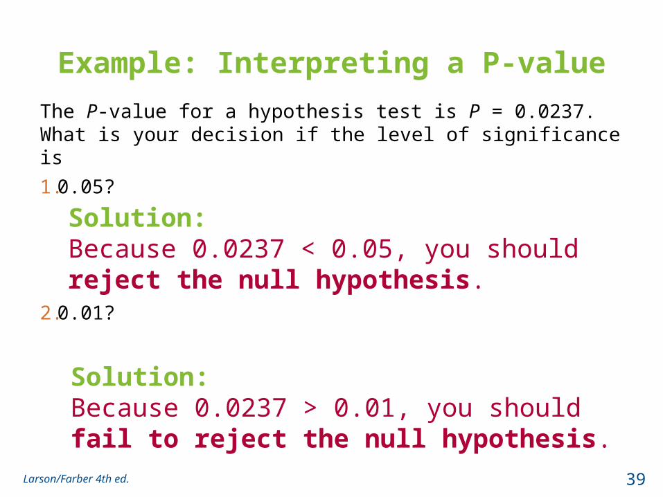
Example: Interpreting a P-value
The P-value for a hypothesis test is P = 0.0237. What is your decision if the level of significance is
1.0.05?
2.0.01?
Solution:Because 0.0237 < 0.05, you should reject the null hypothesis.
Solution:Because 0.0237 > 0.01, you should fail to reject the null hypothesis.
39Larson/Farber 4th ed.

Finding the P-value
After determining the hypothesis test’s standardized test statistic and the test statistic’s corresponding area, do one of the following to find the P-value.
a.For a left-tailed test, P = (Area in left tail).
b.For a right-tailed test, P = (Area in right tail).
c.For a two-tailed test, P = 2(Area in tail of test statistic).
40Larson/Farber 4th ed.

Example: Finding the P-value
Find the P-value for a left-tailed hypothesis test with a test statistic of z = -2.23. Decide whether to reject H0 if the level of significance is α = 0.01.
z0-2.23
P = 0.0129
Solution:For a left-tailed test, P = (Area in left tail)
Because 0.0129 > 0.01, you should fail to reject H0
41Larson/Farber 4th ed.

z0 2.14
Example: Finding the P-value
Find the P-value for a two-tailed hypothesis test with a test statistic of z = 2.14. Decide whether to reject H0 if the level of significance is α = 0.05.
Solution:For a two-tailed test, P = 2(Area in tail of test statistic)
Because 0.0324 < 0.05, you should reject H0
0.9838
1 – 0.9838 = 0.0162
P = 2(0.0162) = 0.0324
42Larson/Farber 4th ed.

Z-Test for a Mean μ
• Can be used when the population is normal and is known, or for any population when the sample size n is at least 30.
• The test statistic is the sample mean
• The standardized test statistic is z
• When n 30, the sample standard deviation s can be substituted for .
xzn
standard error xn
x
43Larson/Farber 4th ed.

Using P-values for a z-Test for Mean μ
1. State the claim mathematically and verbally. Identify the null and alternative hypotheses.
2. Specify the level of significance.
3. Determine the standardized test statistic.
4. Find the area that corresponds to z.
State H0 and Ha.
Identify .
Use Table 4 in Appendix B.
xzn
44Larson/Farber 4th ed.
In Words In Symbols

Using P-values for a z-Test for Mean μ
Reject H0 if P-value is less than or equal to . Otherwise, fail to reject H0.
5. Find the P-value.a. For a left-tailed test, P = (Area in left tail).b. For a right-tailed test, P = (Area in right tail).c. For a two-tailed test, P = 2(Area in tail of test
statistic).6. Make a decision to reject or
fail to reject the null hypothesis.
7. Interpret the decision in the context of the original claim.
45Larson/Farber 4th ed.
In Words In Symbols

Example: Hypothesis Testing Using P-values
In an advertisement, a pizza shop claims that its mean delivery time is less than 30 minutes. A random selection of 36 delivery times has a sample mean of 28.5 minutes and a standard deviation of 3.5 minutes. Is there enough evidence to support the claim at = 0.01? Use a P-value.
46Larson/Farber 4th ed.

Solution: Hypothesis Testing Using P-values
• H0:
• Ha:
• = • Test Statistic:
μ ≥ 30 min
μ < 30 min
0.01
28.5 30
3.5 36
2.57
xz
n
• Decision:
At the 1% level of significance, you have sufficient evidence to conclude the mean delivery time is less than 30 minutes.
z0-2.57
0.0051
• P-value
0.0051 < 0.01Reject H0
47Larson/Farber 4th ed.

Example: Hypothesis Testing Using P-values
You think that the average franchise investment information shown in the graph is incorrect, so you randomly select 30 franchises and determine the necessary investment for each. The sample mean investment is $135,000 with astandard deviation of $30,000. Is there enough evidence to support your claim at = 0.05? Use a P-value.
48Larson/Farber 4th ed.
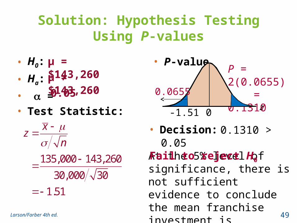
Solution: Hypothesis Testing Using P-values
• H0:
• Ha:
• = • Test Statistic:
μ = $143,260
μ ≠ $143,2600.05
135,000 143,260
30,000 30
1.51
xz
n
• Decision:
At the 5% level of significance, there is not sufficient evidence to conclude the mean franchise investment is different from $143,260.
• P-valueP = 2(0.0655) = 0.1310
0.1310 > 0.05
Fail to reject H0
z0-1.51
0.0655
49Larson/Farber 4th ed.

Rejection Regions and Critical Values
Rejection region (or critical region)
• The range of values for which the null hypothesis is not probable.
• If a test statistic falls in this region, the null hypothesis is rejected.
• A critical value z0 separates the rejection region from the nonrejection region.
50Larson/Farber 4th ed.

Rejection Regions and Critical Values
Finding Critical Values in a Normal Distribution1. Specify the level of significance .2. Decide whether the test is left-, right-, or two-tailed.
3. Find the critical value(s) z0. If the hypothesis test is
a. left-tailed, find the z-score that corresponds to an area of ,
b. right-tailed, find the z-score that corresponds to an area of 1 – ,
c. two-tailed, find the z-score that corresponds to ½ and 1 – ½.
4. Sketch the standard normal distribution. Draw a vertical line at each critical value and shade the rejection region(s).
51Larson/Farber 4th ed.

Example: Finding Critical Values
Find the critical value and rejection region for a two-tailed test with = 0.05.
z0 z0z0
½α = 0.025 ½α = 0.025
1 – α = 0.95
The rejection regions are to the left of -z0 = -1.96 and to the right of z0 = 1.96.
z0 = 1.96-z0 = -1.96
Solution:
52Larson/Farber 4th ed.

Decision Rule Based on Rejection Region
To use a rejection region to conduct a hypothesis test, calculate the standardized test statistic, z. If the standardized test statistic1. is in the rejection region, then reject H0.2. is not in the rejection region, then fail to reject H0.
z0z0
Fail to reject H0.
Reject H0.
Left-Tailed Test
z < z0 z
0 z0
Reject Ho.
Fail to reject Ho.
z > z0
Right-Tailed Test
z0z0
Two-Tailed Testz0z < -z0 z > z0
Reject H0
Fail to reject H0
Reject H0
53Larson/Farber 4th ed.
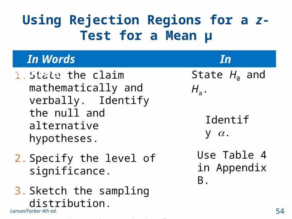
Using Rejection Regions for a z-Test for a Mean μ
1. State the claim mathematically and verbally. Identify the null and alternative hypotheses.
2. Specify the level of significance.
3. Sketch the sampling distribution.
4. Determine the critical value(s).
5. Determine the rejection region(s).
State H0 and Ha.
Identify .
Use Table 4 in Appendix B.
54Larson/Farber 4th ed.
In Words In Symbols

Using Rejection Regions for a z-Test for a Mean μ
6. Find the standardized test statistic.
7. Make a decision to reject or fail to reject the null hypothesis.
8. Interpret the decision in the context of the original claim.
or if 30
use
xz nn
s
.
If z is in the rejection region, reject H0. Otherwise, fail to reject H0.
55Larson/Farber 4th ed.
In Words In Symbols

Example: Testing with Rejection Regions
Employees in a large accounting firm claim that the mean salary of the firm’s accountants is less than that of its competitor’s, which is $45,000. A random sample of 30 of the firm’s accountants has a mean salary of $43,500 with a standard deviation of $5200. At α = 0.05, test the employees’ claim.
56Larson/Farber 4th ed.

Solution: Testing with Rejection Regions
• H0:
• Ha:
• = • Rejection Region:
μ ≥ $45,000
μ < $45,000
0.05
43,500 45,000
5200 30
1.58
xz
n
• Decision:At the 5% level of significance, there is not sufficient evidence to support the employees’ claim that the mean salary is less than $45,000.
• Test Statistic
z0-1.645
0.05
-1.58
-1.645
Fail to reject H0
57Larson/Farber 4th ed.

Example: Testing with Rejection Regions
The U.S. Department of Agriculture reports that the mean cost of raising a child from birth to age 2 in a rural area is $10,460. You believe this value is incorrect, so you select a random sample of 900 children (age 2) and find that the mean cost is $10,345 with a standard deviation of $1540. At α = 0.05, is there enough evidence to conclude that the mean cost is different from $10,460? (Adapted from U.S. Department of Agriculture Center for Nutrition Policy and Promotion)
58Larson/Farber 4th ed.

Solution: Testing with Rejection Regions
• H0:
• Ha:
• = • Rejection Region:
μ = $10,460
μ ≠ $10,460
0.05
10,345 10,460
1540 900
2.24
xz
n
• Decision:At the 5% level of significance, you have enough evidence to conclude the mean cost of raising a child from birth to age 2 in a rural area is significantly different from $10,460.
• Test Statistic
z0-1.96
0.025
1.96
0.025
-1.96 1.96
-2.24
Reject H0
59Larson/Farber 4th ed.

Section 7.2 Summary
• Found P-values and used them to test a mean μ
• Used P-values for a z-test
• Found critical values and rejection regions in a normal distribution
• Used rejection regions for a z-test
60Larson/Farber 4th ed.

Section 7.3
Hypothesis Testing for the Mean (Small Samples)
61Larson/Farber 4th ed.

Section 7.3 Objectives
• Find critical values in a t-distribution
• Use the t-test to test a mean μ
• Use technology to find P-values and use them with a t-test to test a mean μ
62Larson/Farber 4th ed.

Finding Critical Values in a t-Distribution
1. Identify the level of significance .
2. Identify the degrees of freedom d.f. = n – 1.
3. Find the critical value(s) using Table 5 in Appendix B in the row with n – 1 degrees of freedom. If the hypothesis test is
a. left-tailed, use “One Tail, ” column with a negative sign,
b. right-tailed, use “One Tail, ” column with a positive sign,
c. two-tailed, use “Two Tails, ” column with a negative and a positive sign.
63Larson/Farber 4th ed.

Example: Finding Critical Values for t
Find the critical value t0 for a left-tailed test given = 0.05 and n = 21.
Solution:• The degrees of freedom are
d.f. = n – 1 = 21 – 1 = 20.• Look at α = 0.05 in the
“One Tail, ” column. • Because the test is left-
tailed, the critical value is negative.
t0-1.725
0.05
64Larson/Farber 4th ed.

Example: Finding Critical Values for t
Find the critical values t0 and -t0 for a two-tailed test given = 0.05 and n = 26.
Solution:• The degrees of freedom are
d.f. = n – 1 = 26 – 1 = 25.• Look at α = 0.05 in the
“Two Tail, ” column. • Because the test is two-
tailed, one critical value is negative and one is positive.
t0-2.060
0.025
2.060
0.025
65Larson/Farber 4th ed.

t-Test for a Mean μ (n < 30, Unknown)
t-Test for a Mean
• A statistical test for a population mean.
• The t-test can be used when the population is normal or nearly normal, is unknown, and n < 30.
• The test statistic is the sample mean
• The standardized test statistic is t.
• The degrees of freedom are d.f. = n – 1.
xts n
x
66Larson/Farber 4th ed.

Using the t-Test for a Mean μ(Small Sample)
1. State the claim mathematically and verbally. Identify the null and alternative hypotheses.
2. Specify the level of significance.
3. Identify the degrees of freedom and sketch the sampling distribution.
4. Determine any critical value(s).
State H0 and Ha.
Identify .
Use Table 5 in Appendix B.
d.f. = n – 1.
67Larson/Farber 4th ed.
In Words In Symbols

Using the t-Test for a Mean μ(Small Sample)
5. Determine any rejection region(s).
6. Find the standardized test statistic.
7. Make a decision to reject or fail to reject the null hypothesis.
8. Interpret the decision in the context of the original claim.
xts n
If t is in the rejection region, reject H0. Otherwise, fail to reject H0.
68Larson/Farber 4th ed.
In Words In Symbols
Example: Testing μ with a Small Sample
A used car dealer says that the mean price of a 2005 Honda Pilot LX is at least $23,900. You suspect this claim is incorrect and find that a random sample of 14 similar vehicles has a mean price of $23,000 and a standard deviation of $1113. Is there enough evidence to reject the dealer’s claim at α = 0.05? Assume the population is normally distributed. (Adapted from Kelley Blue Book)
69Larson/Farber 4th ed.

Solution: Testing μ with a Small Sample
• H0:
• Ha:
• α =
• df = • Rejection Region:
• Test Statistic:
• Decision:
μ ≥ $23,900μ < $23,900
0.0514 – 1 = 13
23,000 23,9003.026
1113 14
xt
s n
t0-1.771
0.05
-3.026
-1.771
At the 0.05 level of significance, there is enough evidence to reject the claim that the mean price of a 2005 Honda Pilot LX is at least $23,900
Reject H0
70Larson/Farber 4th ed.

Example: Testing μ with a Small Sample
An industrial company claims that the mean pH level of the water in a nearby river is 6.8. You randomly select 19 water samples and measure the pH of each. The sample mean and standard deviation are 6.7 and 0.24, respectively. Is there enough evidence to reject the company’s claim at α = 0.05? Assume the population is normally distributed.
71Larson/Farber 4th ed.

Solution: Testing μ with a Small Sample
• H0:
• Ha:
• α =
• df = • Rejection Region:
• Test Statistic:
• Decision:
μ = 6.8μ ≠ 6.8
0.05
19 – 1 = 18
6.7 6.81.816
0.24 19
xt
s n
At the 0.05 level of significance, there is not enough evidence to reject the claim that the mean pH is 6.8.t
0-2.101
0.025
2.101
0.025
-2.101 2.101
-1.816
Fail to reject H0
72Larson/Farber 4th ed.
Example: Using P-values with t-Tests
The American Automobile Association claims that the mean daily meal cost for a family of four traveling on vacation in Florida is $118. A random sample of 11 such families has a mean daily meal cost of $128 with a standard deviation of $20. Is there enough evidence to reject the claim at α = 0.10? Assume the population is normally distributed. (Adapted from American Automobile Association)
73Larson/Farber 4th ed.

Solution: Using P-values with t-Tests
• H0:
• Ha:
• Decision:
μ = $118μ ≠ $118
TI-83/84set up: Calculate: Draw:
Fail to reject H0. At the 0.10 level of significance, there is not enough evidence to reject the claim that the mean daily meal cost for a family of four traveling on vacation in Florida is $118.
74Larson/Farber 4th ed.
0.1664 > 0.10

Section 7.3 Summary
• Found critical values in a t-distribution
• Used the t-test to test a mean μ
• Used technology to find P-values and used them with a t-test to test a mean μ
75Larson/Farber 4th ed.

Section 7.4
Hypothesis Testing for Proportions
76Larson/Farber 4th ed.

Section 7.4 Objectives
• Use the z-test to test a population proportion p
77Larson/Farber 4th ed.

z-Test for a Population Proportion
z-Test for a Population Proportion
• A statistical test for a population proportion.
• Can be used when a binomial distribution is given such that np 5 and nq 5.
• The test statistic is the sample proportion .
• The standardized test statistic is z.
ˆ
ˆ
ˆ ˆp
p
p p pzpq n
p̂
78Larson/Farber 4th ed.

Using a z-Test for a Proportion p
1. State the claim mathematically and verbally. Identify the null and alternative hypotheses.
2. Specify the level of significance.
3. Sketch the sampling distribution.
4. Determine any critical value(s).
State H0 and Ha.
Identify .
Use Table 5 in Appendix B.
Verify that np ≥ 5 and nq ≥ 5
79Larson/Farber 4th ed.
In Words In Symbols

Using a z-Test for a Proportion p
5. Determine any rejection region(s).
6. Find the standardized test statistic.
7. Make a decision to reject or fail to reject the null hypothesis.
8. Interpret the decision in the context of the original claim.
If z is in the rejection region, reject H0. Otherwise, fail to reject H0.
p̂ pzpq n
80Larson/Farber 4th ed.
In Words In Symbols

Example: Hypothesis Test for Proportions
Zogby International claims that 45% of people in the United States support making cigarettes illegal within the next 5 to 10 years. You decide to test this claim and ask a random sample of 200 people in the United States whether they support making cigarettes illegal within the next 5 to 10 years. Of the 200 people, 49% support this law. At α = 0.05 is there enough evidence to reject the claim?
Solution:•Verify that np ≥ 5 and nq ≥ 5.
np = 200(0.45) = 90 and nq = 200(0.55) = 11081Larson/Farber 4th ed.
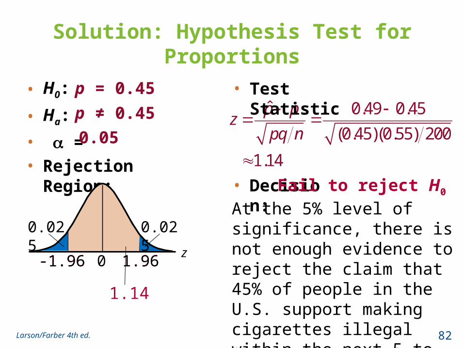
Solution: Hypothesis Test for Proportions
• H0:
• Ha:
• = • Rejection Region:
p = 0.45
p ≠ 0.45
0.05
ˆ 0.49 0.45
(0.45)(0.55) 200
1.14
p pz
pq n
• Decision:At the 5% level of significance, there is not enough evidence to reject the claim that 45% of people in the U.S. support making cigarettes illegal within the next 5 to 10 years.
• Test Statistic
z0-1.96
0.025
1.96
0.025
-1.96 1.96
1.14
Fail to reject H0
82Larson/Farber 4th ed.
Example: Hypothesis Test for Proportions
The Pew Research Center claims that more than 55% of U.S. adults regularly watch their local television news. You decide to test this claim and ask a random sample of 425 adults in the United States whether they regularly watch their local television news. Of the 425 adults, 255 respond yes. At α = 0.05 is there enough evidence to support the claim?
Solution:•Verify that np ≥ 5 and nq ≥ 5.
np = 425(0.55) ≈ 234 and nq = 425 (0.45) ≈ 191
83Larson/Farber 4th ed.

Solution: Hypothesis Test for Proportions
• H0:
• Ha:
• = • Rejection Region:
p ≤ 0.55
p > 0.55
0.05
ˆ 255 425 0.55
(0.55)(0.45) 425
2.07
p pz
pq n
• Decision:At the 5% level of significance, there is enough evidence to support the claim that more than 55% of U.S. adults regularly watch their local television news.
• Test Statistic
z0 1.645
0.05
2.07
1.645
Reject H0
84Larson/Farber 4th ed.

Section 7.4 Summary
• Used the z-test to test a population proportion p
85Larson/Farber 4th ed.

Section 7.5
Hypothesis Testing for Variance and Standard Deviation
86Larson/Farber 4th ed.

Section 7.5 Objectives
• Find critical values for a χ2-test
• Use the χ2-test to test a variance or a standard deviation
87Larson/Farber 4th ed.

Finding Critical Values for the χ2-Test
1. Specify the level of significance .
2. Determine the degrees of freedom d.f. = n – 1.
3. The critical values for the χ2-distribution are found in Table 6 of Appendix B. To find the critical value(s) for a
a. right-tailed test, use the value that corresponds to d.f. and .
b. left-tailed test, use the value that corresponds to d.f. and 1 – .
c. two-tailed test, use the values that corresponds to d.f. and ½ and d.f. and 1 – ½.
88Larson/Farber 4th ed.
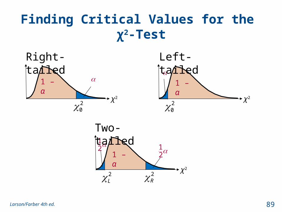
Finding Critical Values for the χ2-Test
χ2
12
2L 2
R
12
1 – α
χ2
20
1 – α
χ2
20
1 – α
Right-tailed Left-tailed
Two-tailed
89Larson/Farber 4th ed.

Example: Finding Critical Values for χ2
Find the critical χ2-value for a left-tailed test whenn = 11 and = 0.01.
Solution:•Degrees of freedom: n – 1 = 11 – 1 = 10 d.f. •The area to the right of the critical value is 1 – = 1 – 0.01 = 0.99.
From Table 6, the critical value is .
20 2.558
χ2
0.01
20
20 2.558
90Larson/Farber 4th ed.

Example: Finding Critical Values for χ2
Find the critical χ2-value for a two-tailed test when n = 13 and = 0.01.
Solution:•Degrees of freedom: n – 1 = 13 – 1 = 12 d.f. •The areas to the right of the critical values are
From Table 6, the critical values are and
02
051
.0
11 9
20.9 5
2L 2
Rχ2
1 0.0052
1 0.0052
2 3.074L 2 28.299R 2 3.074L
2 28.299R 91Larson/Farber 4th ed.

The Chi-Square Test
χ2-Test for a Variance or Standard Deviation
• A statistical test for a population variance or standard deviation.
• Can be used when the population is normal.
• The test statistic is s2.
• The standardized test statistic
follows a chi-square distribution with degrees of freedom d.f. = n – 1.
22
2( 1)n s
92Larson/Farber 4th ed.

Using the χ2-Test for a Variance or Standard Deviation
1. State the claim mathematically and verbally. Identify the null and alternative hypotheses.
2. Specify the level of significance.
3. Determine the degrees of freedom and sketch the sampling distribution.
4. Determine any critical value(s).
State H0 and Ha.
Identify .
Use Table 6 in Appendix B.
d.f. = n – 1
93Larson/Farber 4th ed.
In Words In Symbols

Using the χ2-Test for a Variance or Standard Deviation
22
2( 1)n s
If χ2 is in the rejection region, reject H0. Otherwise, fail to reject H0.
5. Determine any rejection region(s).
6. Find the standardized test statistic.
7. Make a decision to reject or fail to reject the null hypothesis.
8. Interpret the decision in the context of the original claim.
94Larson/Farber 4th ed.
In Words In Symbols

Example: Hypothesis Test for the Population Variance
A dairy processing company claims that the variance of the amount of fat in the whole milk processed by the company is no more than 0.25. You suspect this is wrong and find that a random sample of 41 milk containers has a variance of 0.27. At α = 0.05, is there enough evidence to reject the company’s claim? Assume the population is normally distributed.
95Larson/Farber 4th ed.

Solution: Hypothesis Test for the Population Variance
• H0:
• Ha:
• α =
• df =
• Rejection Region:
• Test Statistic:
• Decision:
σ2 ≤ 0.25
σ2 > 0.25
0.0541 – 1 = 40
22
2
( 1) (41 1)(0.27)
0.2543.2
n s
Fail to Reject H0
At the 5% level of significance, there is not enough evidence to reject the company’s claim that the variance of the amount of fat in the whole milk is no more than 0.25.
χ2
0.05
55.75855.75843.2
96Larson/Farber 4th ed.

Example: Hypothesis Test for the Standard Deviation
A restaurant claims that the standard deviation in the length of serving times is less than 2.9 minutes. A random sample of 23 serving times has a standard deviation of 2.1 minutes. At α = 0.10, is there enough evidence to support the restaurant’s claim? Assume the population is normally distributed.
97Larson/Farber 4th ed.

Solution: Hypothesis Test for the Standard Deviation
• H0:
• Ha:
• α =
• df =
• Rejection Region:
• Test Statistic:
• Decision:
σ ≥ 2.9 min.
σ < 2.9 min.
0.1023 – 1 = 22
2 22
2 2
( 1) (23 1)(2.1)
2.911.536
n s
Reject H0
At the 10% level of significance, there is enough evidence to support the claim that the standard deviation for the length of serving times is less than 2.9 minutes.11.536
14.042χ2
0.10
14.042
98Larson/Farber 4th ed.

Example: Hypothesis Test for the Population Variance
A sporting goods manufacturer claims that the variance of the strength in a certain fishing line is 15.9. A random sample of 15 fishing line spools has a variance of 21.8. At α = 0.05, is there enough evidence to reject the manufacturer’s claim? Assume the population is normally distributed.
99Larson/Farber 4th ed.

5.629χ2
1 0.0252
26.119
Solution: Hypothesis Test for the Population Variance
• H0:
• Ha:
• α =
• df =
• Rejection Region:
• Test Statistic:
• Decision:
σ2 = 15.9
σ2 ≠ 15.9
0.0515 – 1 = 14
22
2
( 1) (15 1)(21.8)
15.919.194
n s
Fail to Reject H0
At the 5% level of significance, there is not enough evidence to reject the claim that the variance in the strength of the fishing line is 15.9.
5.62919.194
26.119
100Larson/Farber 4th ed.

Section 7.5 Summary
• Found critical values for a χ2-test
• Used the χ2-test to test a variance or a standard deviation
101Larson/Farber 4th ed.