Chapter 7

Linear Programming Models

Part One

Basis of Linear Programming Linear Program formulation

Linear Programming (LP)

Linear programming is a optimization model with an objective (in a linear function) and a set of limitations (in linear constraints).

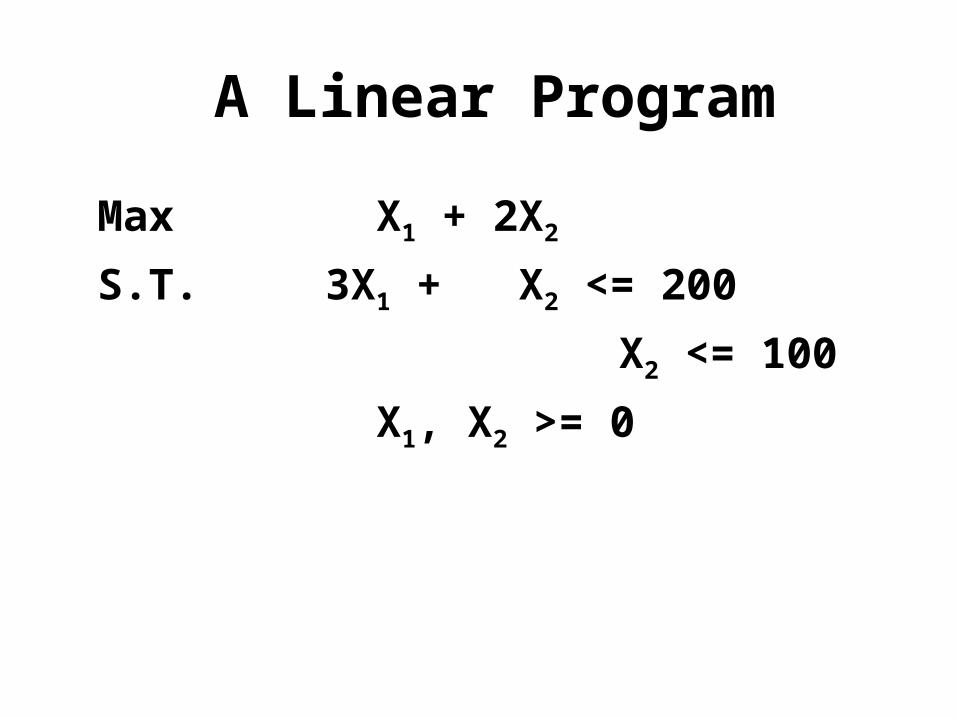
A Linear Program

Max X1 + 2X2

S.T. 3X1 + X2 <= 200

X2 <= 100

X1, X2 >= 0

LP Components

Decision variables - their values are to be found in the solution.

One objective function – tells our goal.

Constraints - reflect limitations. Only linear terms are allowed.

Linear Terms

A term is linear if it contains one variable with exponent one, or if it is a constant.

Examples of linear terms: 3.5X 68.83 (3.78)6X1

Examples of non-linear terms:– 5X2 X1X2 sin X X3

– X2.5 Log X

42X 122

7X

X8

5 X

Format of a Linear Program

Align columns of inequality signs, variable terms, and constants.

Variable terms are at left, constant terms are at right (called right-hand-side, RHS).

Non-negative constraints must be there.

LP Solution A solution is a set of values each for a

variable. A feasible solution satisfies all

constraints. An infeasible solution violates at least one

constraint. The optimal solution is a feasible solution

that makes the objective function value maximized (or minimized).

LP Solution Methods Trial-and-Error

(brute force) Graphic Method

(Won’t work if more than 2 variables)

Simplex Method (by George Dentzig)

(Elegant, but time-taking if by hand) Computerized simplex method

(We’ll use it!)

George Dantzig1914-2005

Inventor of Simplex Method.Professor of Operations

Research and Computer Science

at Stanford University.

To Solve a Problem by Linear Programming

Formulate the problem into a linear program (LP).

Enter the LP into QM. QM solves LP and provide the optimal

solution.

Formulate a Problem into LP

To formulate a decision making problem into a linear program:– Understand the problem thoroughly;– Define decision variables in

unambiguous terms;– Describe the problem with one

objective function and a few constraints, in terms of the variables.

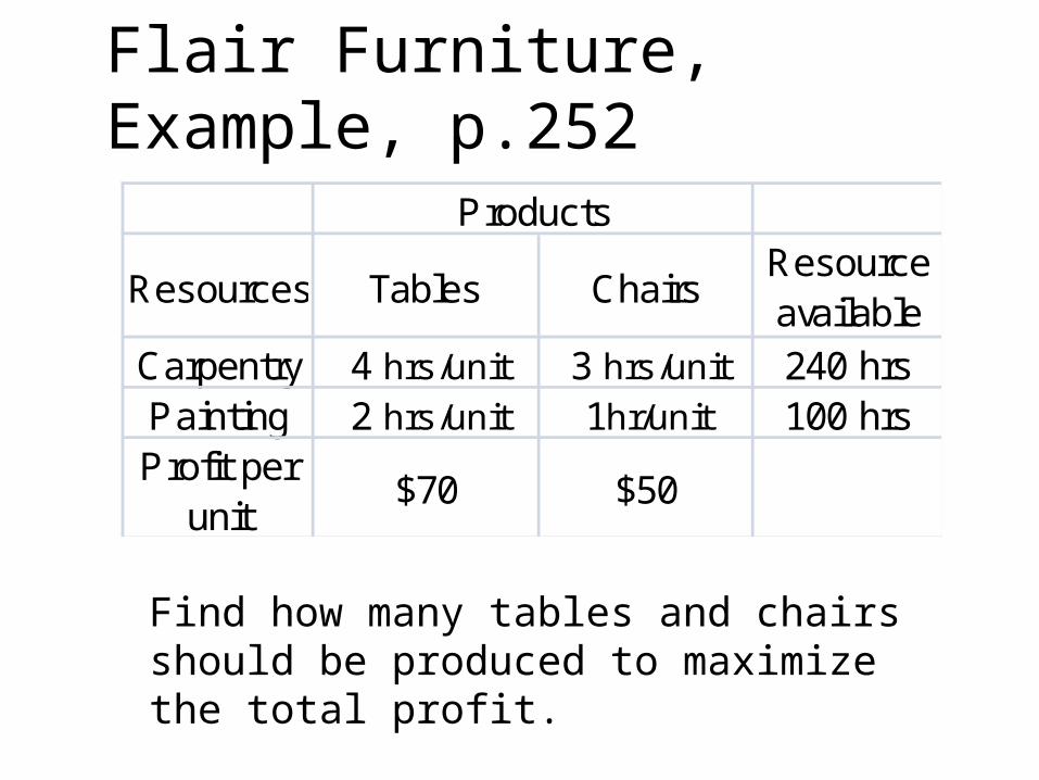
Flair Furniture, Example, p.252

Products

Resources Tables ChairsResource available

Carpentry 4 hrs/unit 3 hrs/unit 240 hrsPainting 2 hrs/unit 1hr/unit 100 hrsProfit per

unit$70 $50

Find how many tables and chairs should be produced to maximize the total profit.

Flair Furniture, Example, p.252

Definitions of variables:

LP formulation:

Solution from QM

Tips of Formulating LP

What are variables?– Those amounts you want to decide.

What is the ‘objective’?– Profit (or cost) you do not know but you

want to maximize (or minimize). What are ‘constraints’?

– Restrictions of reaching your ‘objective’.

Holiday Meal Turkey Ranch, p.270Composition (oz/pound)

IngredientBrand 1

feedBrand 2

feedMin. req.

per turkeyA 5 10 90 ozB 4 3 48 ozC 0.5 0 1.5 oz

Cost per pound

2 cents 3 cents

Find how many pounds of brand 1feed and brand 2 feed should be purchased with lowest cost, which meet the minimum requirements of a turkey for each ingredient.

Holiday Meal Turkey Ranch, p.270

Definitions of variables:

LP formulation:

Solution from QM:

Formulating

To formulate a business problem into a linear program is to re-describe the problem with a ‘language’ that a computer understands.

The key concern of formulation is: – whether the LP tells the story exactly the same as

the original one. Formulating is synonymous with ‘describing’

and ‘translating’. It is NOT ‘solving’.

“Team Work”

The process of solving a business problem by using linear programming is a team work between us and computers:– We formulate the problem in LP so that

computers can understand;– Computers solve the LP, providing us

with the solution to the problem.

Irregular LP Problems

A regular LP has one optimal solution. An irregular LP has no or many optimal

solutions:– Infeasible problem– Unbounded problem – Multiple optimal solutions

Redundancy refers to having extra and un-useful constraints.

Part Two

Shadow Price (Dual Value) Sensitivity Analysis

Dual Price

Each dual price is associated with a constraint. It is the amount of improvement in the objective function value that is caused by a one-unit increase in the RHS of the constraint.

It is also called Shadow Price.

In a product-mix problem

As in the Flair Furniture example, a dual price is:– the contribution of an additional unit of a

resource to the objective function value (total profit), i.e.,

– the marginal value of a resource, i.e., – The highest “price” the company would be

willing to pay for one additional unit of a resource.

Primal and Dual in LP

Each linear program has another associated with it. They are called a pair of primal and dual.

The dual LP is the “transposition” of the primal LP.

Primal and dual have equal optimal objective function values.

The solution of the dual is the dual prices of the primal, and vice versa.

More on Dual Price:

A dual price can be negative, which shows a negative ( or worse off) contribution to the objective function value by an additional unit of RHS increase of the constraint.

Sensitivity Analysis (S.A.)

S.A. is the analysis of the effect of parameter changes on the optimal solution.

S. A. is conducted after the optimal solution is obtained.

S.A. on Objective Coefficients

Sensitivity range for an objective coefficient is the range of values over which the coefficient can change without changing the current optimal solution.

S.A. on RHS

Sensitivity range for a RHS value is the range of values over which the RHS value can change without changing the dual prices.

S.A. on other changes

To see sensitivities on following changes, one must solve the changed LP again: – Changing technological (constraint)

coefficients– Adding a new constraint– Adding a new variable

Why doing S.A.? LP is used for decision making on

something in the future. Rarely does a manager know all of the

parameters exactly. Many parameters are inaccurate “estimates” when a model is formed and solved.

We want to see to what extent the optimal solution is stable to the inaccurate parameters.

Sensitive or In-sensitive? Do we want a model more sensitive or less

sensitive to the inaccuracies (changes) of parameters in it ?

Answer: Less sensitive.

Why? – An optimal solution that is insensitive to

inaccuracies of parameters is more likely valid in the real world situation.