Chapter 7Localization & Positioning

112/04/191

Means for a node to determine its physical position with respect to some coordinate system (50, 27) or symbolic location (in a living room)

Using the help of Anchor nodes that know their position Directly adjacent nodes Over multiple hops

Goals of this chapter

112/04/192

7.1 Properties of localization and positioning procedures

7.2 Possible approaches 7.3 Mathematical basics for the lateration problem 7.4 Positioning in multi-hop environments 7.5 Positioning assisted by anchors

Outline

112/04/193

Physical position versus logical location Coordinate system: position Symbolic reference: location

Absolute versus relative coordinate Centralized or distributed computation Localized versus centralized computation Limitations: GPS for example, does not work indoors Scale (indoors, outdoors, global, …)

7.1 Properties of localization and positioning procedures

112/04/194

Accuracy how close is an estimated position to the real

position? Precision

the ratio with which a given accuracy is reached Costs, energy consumption, …

Properties of localization and positioning procedures (cont.)

112/04/195

Proximity A node wants to determine its position or location in the proximity of an

anchor

(Tri-/Multi-) lateration and angulation Lateration : when distances between nodes are used Angulation: when angles between nodes are used

Scene analysis The most evident form of it is to analyze pictures taken by a camera Other measurable characteristic ‘fingerprints’ of a given location can be

used for scene analysis e.g., RADAR

Bounding box to bound the possible positions of a node

7.2 Possible approaches

112/04/196

Using information of a node’s neighborhood Exploit finite range of wireless communication

e.g., easy to determine location in a room with infrared (room number announcements)

Proximity (range-free approach)

112/04/197

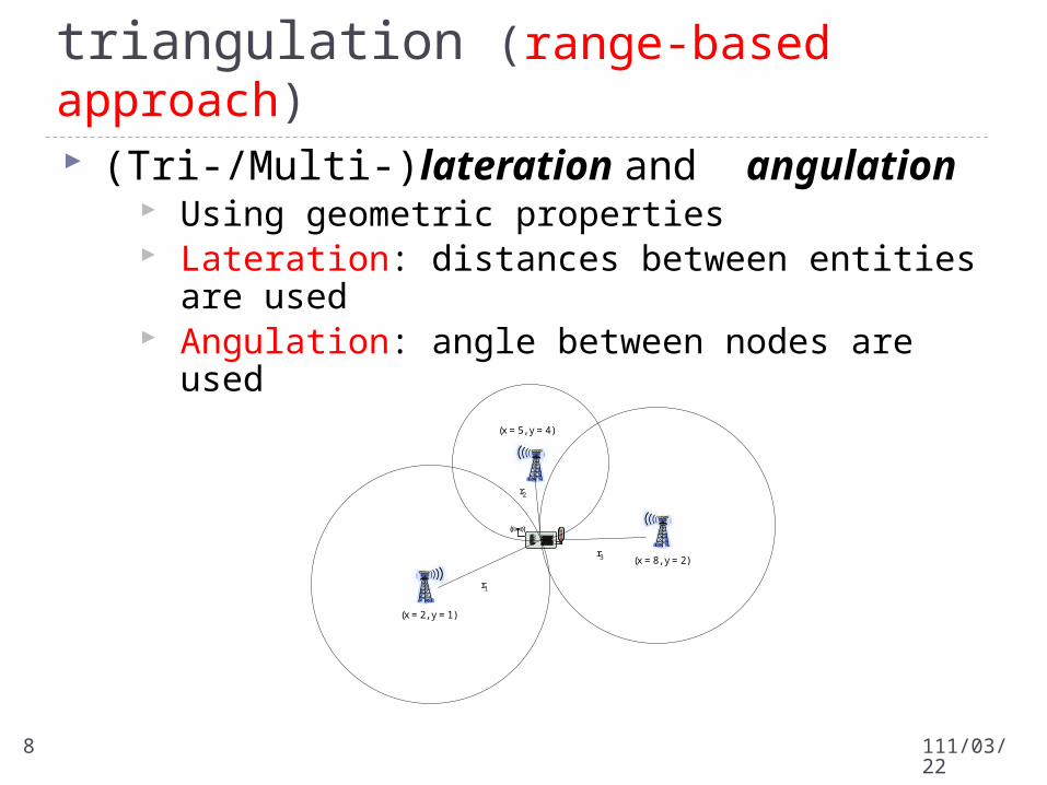
(Tri-/Multi-)lateration and angulation Using geometric properties Lateration: distances between entities are used Angulation: angle between nodes are used

(x = 2, y = 1)

(x = 8, y = 2)

(x = 5, y = 4)

r1

r2

r3

Trilateration and triangulation (range-based approach)

112/04/198

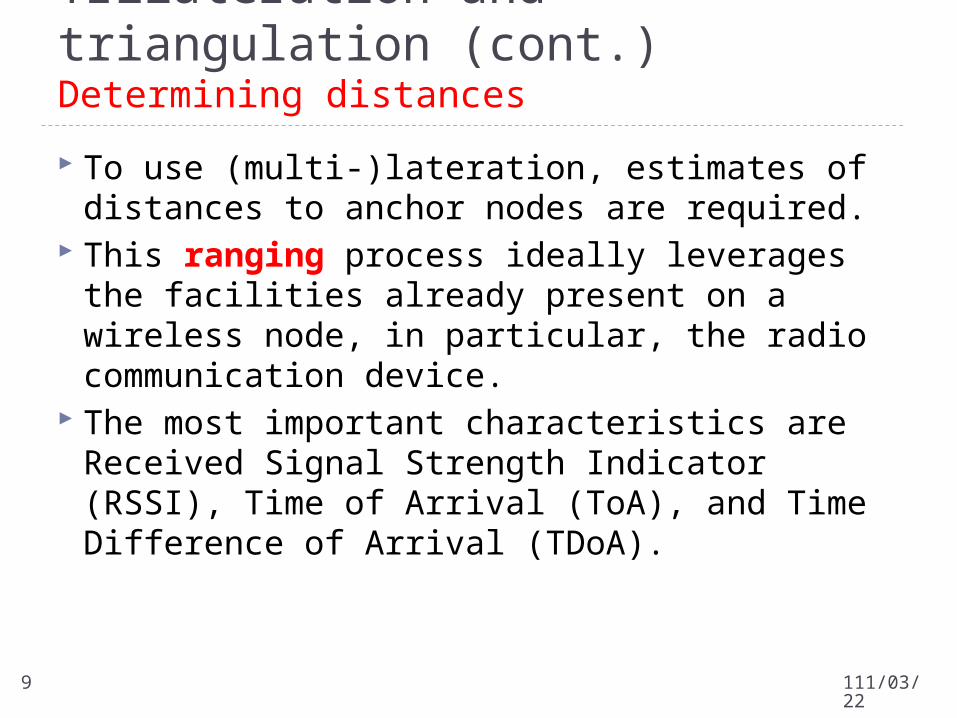
To use (multi-)lateration, estimates of distances to anchor nodes are required.

This ranging process ideally leverages the facilities already present on a wireless node, in particular, the radio communication device.

The most important characteristics are Received Signal Strength Indicator (RSSI), Time of Arrival (ToA), and Time Difference of Arrival (TDoA).

Trilateration and triangulation (cont.)Determining distances

112/04/199

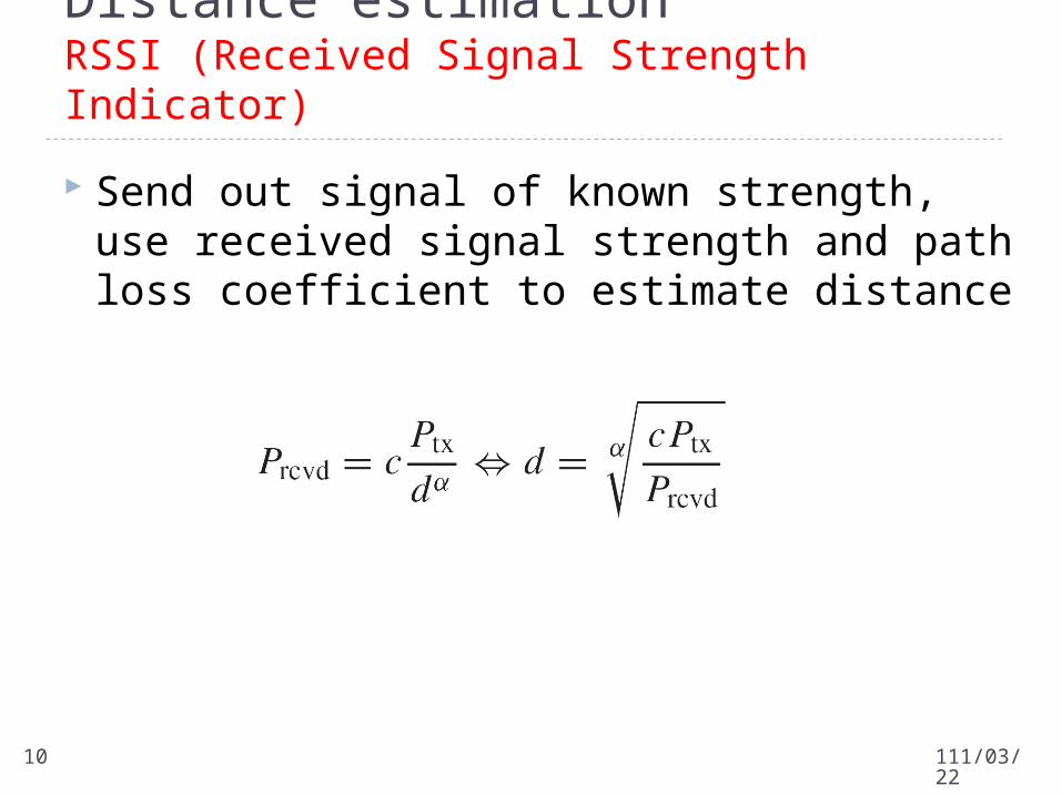
Send out signal of known strength, use received signal strength and path loss coefficient to estimate distance

Distance estimation RSSI (Received Signal Strength Indicator)

112/04/1910

Problem: Highly error-prone process : Caused by fast fading, mobility of the environment Solution: repeated measurement and filtering out incorrect

values by statistical techniques Cheap radio transceivers are often not calibrated

Same signal strength result in different RSSI Actual transmission power different from the intended power Combination with multipath fading Signal attenuation along an indirect path is higher than along

a direct path Solution: No!

Distance estimationRSSI (cont.)

112/04/1911

Distance estimationRSSI (cont.)

DistanceDistance Signal strength

PD

F

PD

F

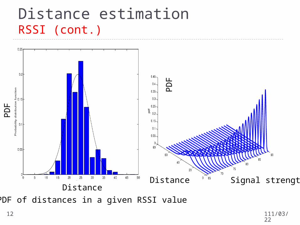
PDF of distances in a given RSSI value

112/04/1912

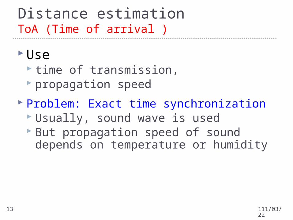
Use time of transmission, propagation speed

Problem: Exact time synchronization Usually, sound wave is used But propagation speed of sound depends on

temperature or humidity

Distance estimation ToA (Time of arrival )

112/04/1913

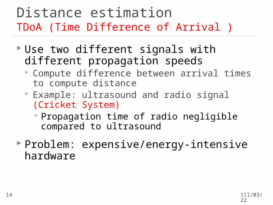
Use two different signals with different propagation speeds Compute difference between arrival times to compute

distance Example: ultrasound and radio signal (Cricket System)

Propagation time of radio negligible compared to ultrasound

Problem: expensive/energy-intensive hardware

Distance estimationTDoA (Time Difference of Arrival )

112/04/1914

RADAR system: Comparing the received signal characteristics from multiple anchors with premeasured and stored characteristics values.

Radio environment has characteristic “fingerprints” The necessary off-line deployment for measuring the

signal landscape cannot always be accommodated in practical systems.

Scene analysis

112/04/1915

Bounding Box

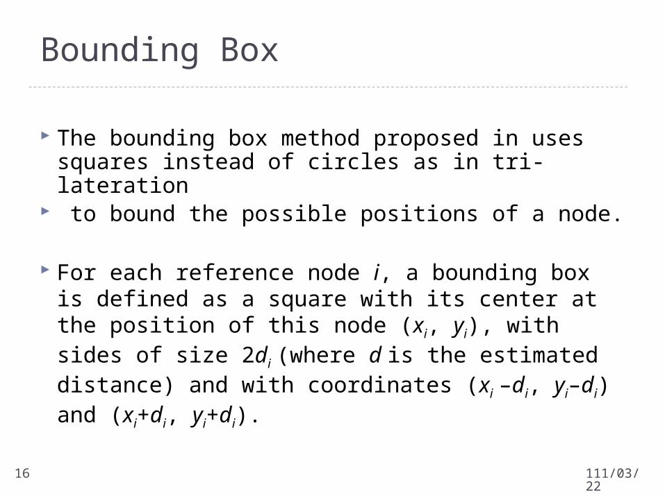
The bounding box method proposed in uses squares instead of circles as in tri-lateration

to bound the possible positions of a node.

For each reference node i, a bounding box is defined as a square with its center at the position of this node (xi, yi), with sides of size 2di (where d is the estimated distance) and with coordinates (xi –di, yi–di) and (xi+di, yi+di).

112/04/1916

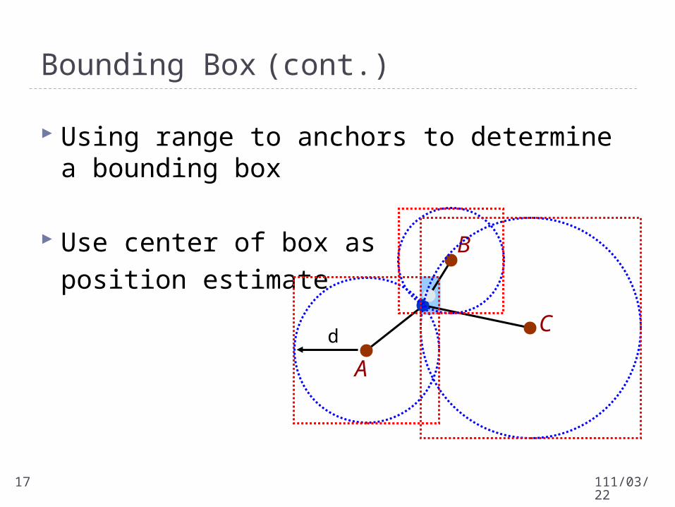
Bounding Box (cont.)

Using range to anchors to determine a bounding box

Use center of box as

position estimate

C

A

B

d

112/04/1917

References N. Bulusu, J. Heidemann, and D. Estrin. “GPS-Less Low Cost

Outdoor Localization For Very Small Devices,” IEEE Personal Communications Magazine, 7(5): 28–34, 2000.

C. Savarese, J. Rabay, and K. Langendoen. “Robust Positioning Algorithms for Distributed Ad-Hoc Wireless Sensor Networks,” In Proceedings of the Annual USENIX Technical Conference, Monterey, CA, 2002.

A. Savvides, C.-C. Han, and M. Srivastava. “Dynamic Fine-Grained Localization in Ad-Hoc Networks of Sensors,” Proceedings of the 7th Annual International Conference on Mobile Computing and Networking, pages 166–179. ACM press, Rome, Italy, July 2001.

S. Simic and S. Sastry, “Distributed localization in wireless ad hoc networks,” UC Berkeley, Tech. rep. UCB/ERL M02/26, 2002.

112/04/1918

7.3 Mathematical basics for the lateration problem

112/04/1919

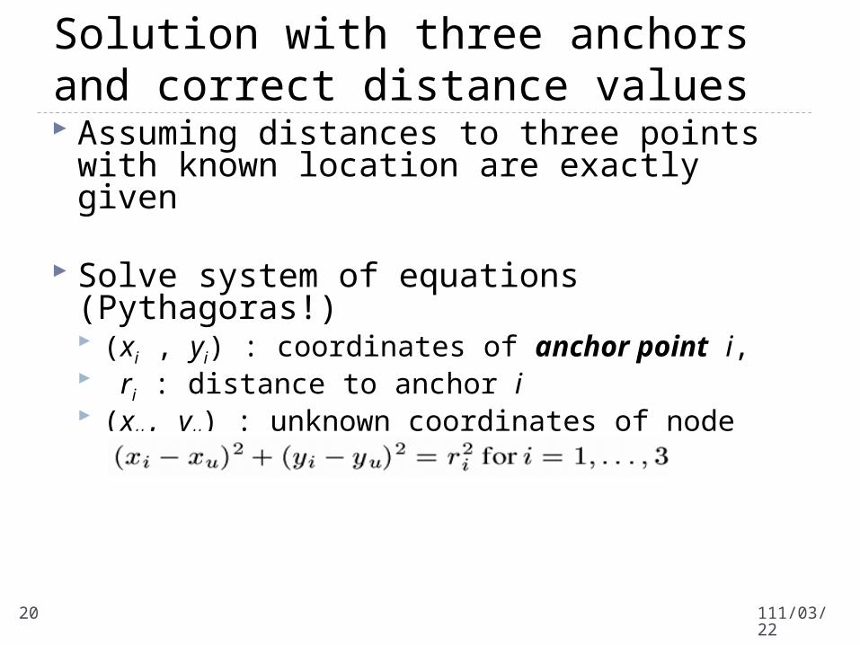
Solution with three anchors and correct distance values Assuming distances to three points with known

location are exactly given

Solve system of equations (Pythagoras!) (xi , yi) : coordinates of anchor point i, ri : distance to anchor i (xu, yu) : unknown coordinates of node

112/04/1920

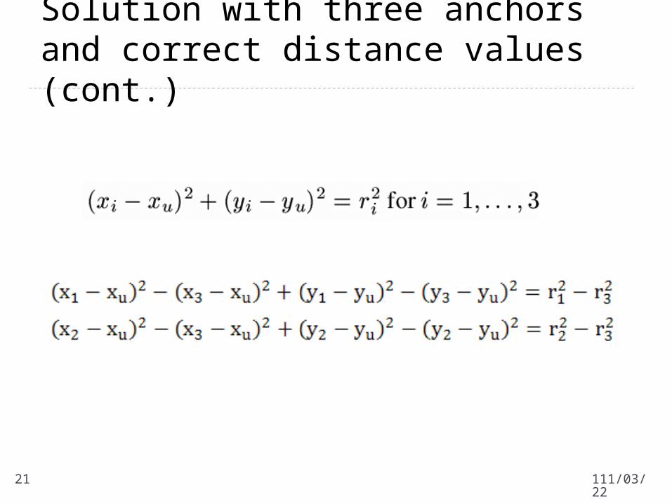
Solution with three anchors and correct distance values (cont.)

112/04/1921

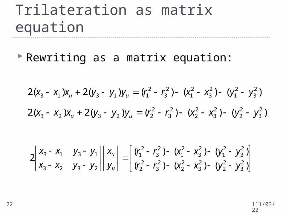
Rewriting as a matrix equation:

Trilateration as matrix equation

)()()(

)()()(2

23

22

23

22

23

22

23

21

23

21

23

21

2323

1313

yyxxrr

yyxxrr

y

x

yyxx

yyxx

u

u

)()()()(2)(2 23

21

23

21

23

211313 yyxxrryyyxxx uu

)()()()(2)(2 23

22

23

22

23

222323 yyxxrryyyxxx uu

112/04/1922

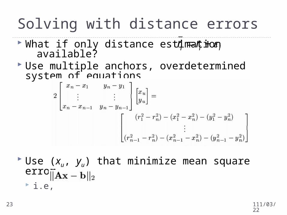
What if only distance estimation available? Use multiple anchors, overdetermined system of

equations

Use (xu, yu) that minimize mean square error, i.e,

Solving with distance errors

iii rr _

112/04/1923

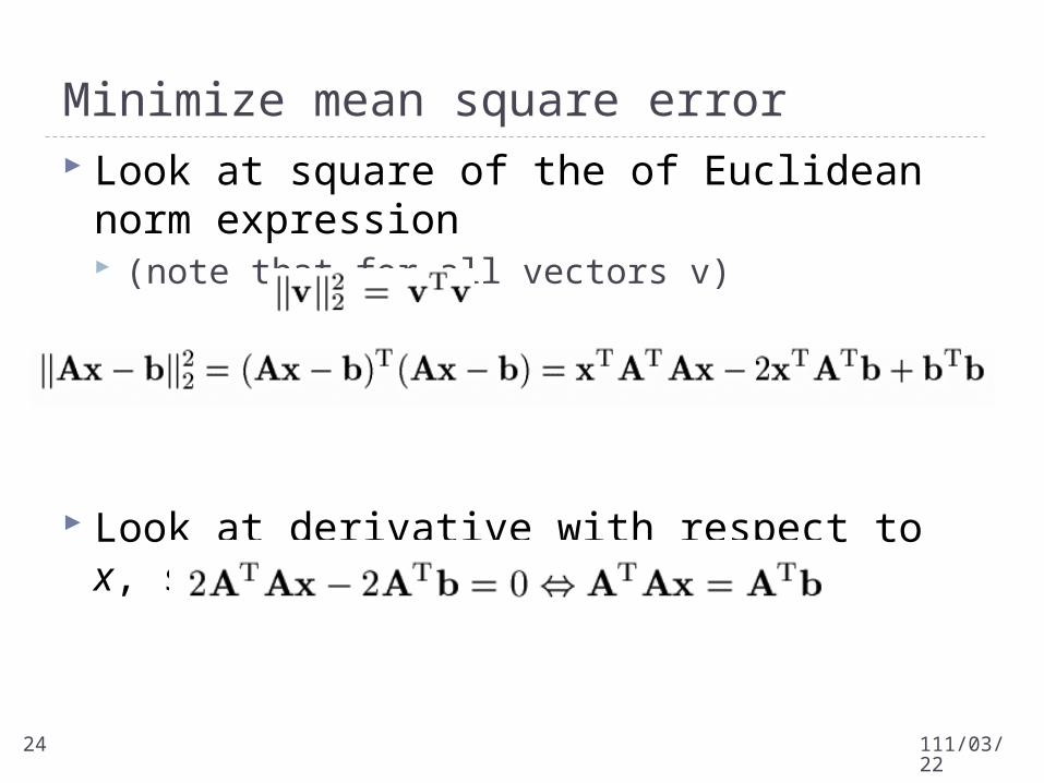
Look at square of the of Euclidean norm expression (note that for all vectors v)

Look at derivative with respect to x, set it equal to 0

Minimize mean square error

112/04/1924

7.4 Positioning in multi-hop environments

112/04/1925

Assume that the positions of n anchors are known and the positions of m nodes is to be determined, that connectivity between any two nodes is only possible if nodes are at most R distance units apart, and that the connectivity between any two nodes is also known

The fact that two nodes are connected introduces a constraint to the feasibility problem – for two connected nodes, it is impossible to choose positions that would place them further than R away

Connectivity in a multi-hop network

112/04/1926

Multi-hop range estimation

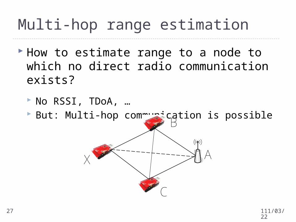
How to estimate range to a node to which no direct radio communication exists?

No RSSI, TDoA, … But: Multi-hop communication is possible

A

C

B

X

112/04/1927

Multi-hop range estimation (cont.)

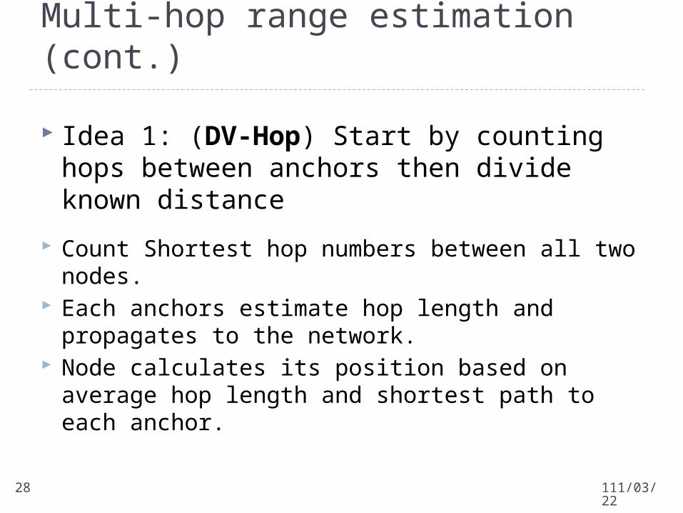
Idea 1: (DV-Hop) Start by counting hops between anchors then divide known distance

Count Shortest hop numbers between all two nodes. Each anchors estimate hop length and propagates to the

network. Node calculates its position based on average hop length and

shortest path to each anchor.

112/04/1928

DV Hop

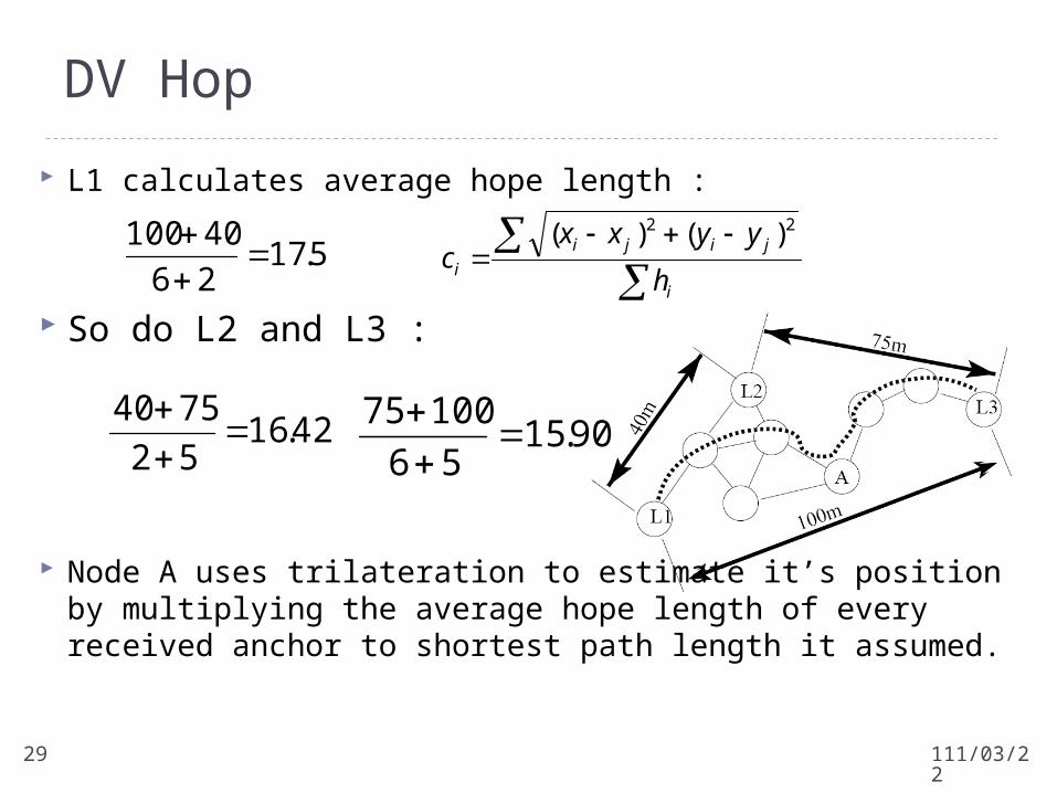
L1 calculates average hope length :

So do L2 and L3 :

Node A uses trilateration to estimate it’s position by multiplying the average hope length of every received anchor to shortest path length it assumed.

5.1726

40100

42.1652

7540

90.1556

10075

i

jiji

i h

yyxxc

22 )()(

112/04/1929

DV-Distance

Idea 2: If range estimates between neighbors exist, use them to improve total length of route estimation in previous method (DV-Distance)

Distance between neighboring nodes is measured using radio signal strength and is propagated in meters rather than in hops.

The algorithm uses the same method to estimate but shortest distance length are assumed.

112/04/1930

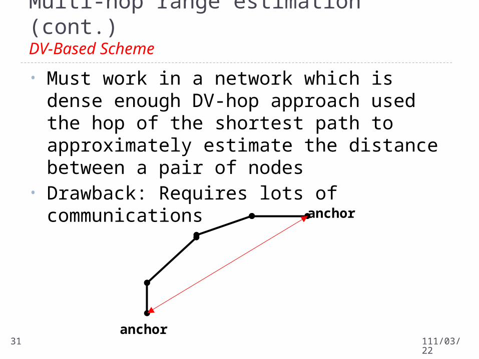
• Must work in a network which is dense enough DV-hop approach used the hop of the shortest path to approximately estimate the distance between a pair of nodes

• Drawback: Requires lots of communications

anchor

anchor

Multi-hop range estimation (cont.) DV-Based Scheme

112/04/1931

Number of anchors Euclidean method increase accuracy as the number of

anchors goes up The “distance vector”-like methods are better suited for a

low-ratio of anchors Uniformly distributed network

Distance vector methods perform less well in non-uniformly networks

Euclidean method is not very sensitive to this effect

Discussion

112/04/1932

7.5 Positioning assisted by anchors

112/04/1933

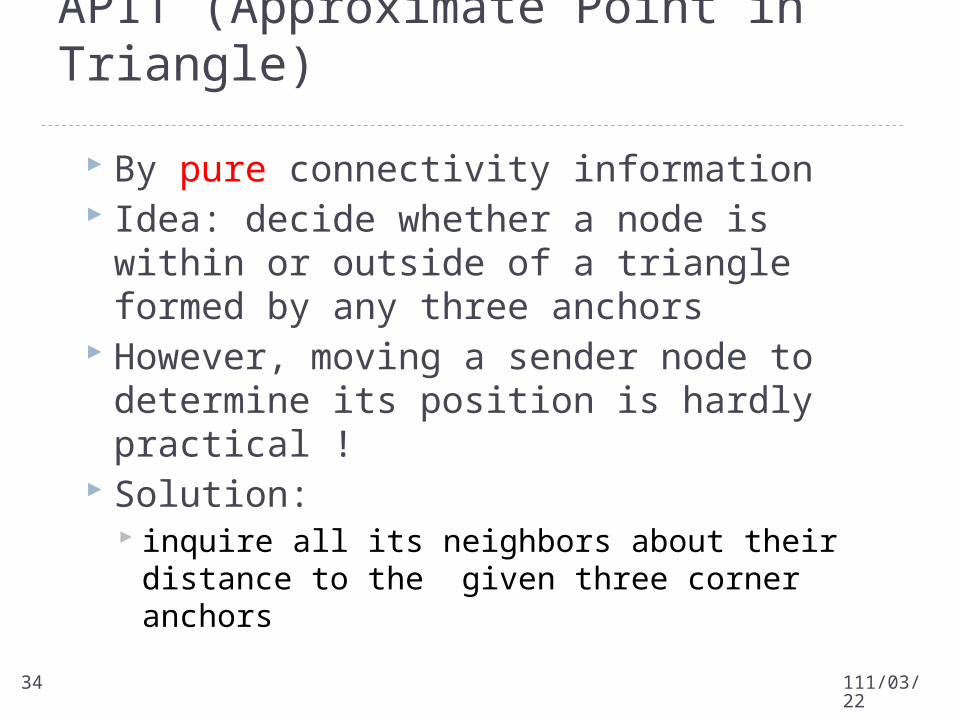
By pure connectivity information Idea: decide whether a node is within or outside of a

triangle formed by any three anchors However, moving a sender node to determine its

position is hardly practical ! Solution:

inquire all its neighbors about their distance to the given three corner anchors

APIT (Approximate Point in Triangle)

112/04/1934

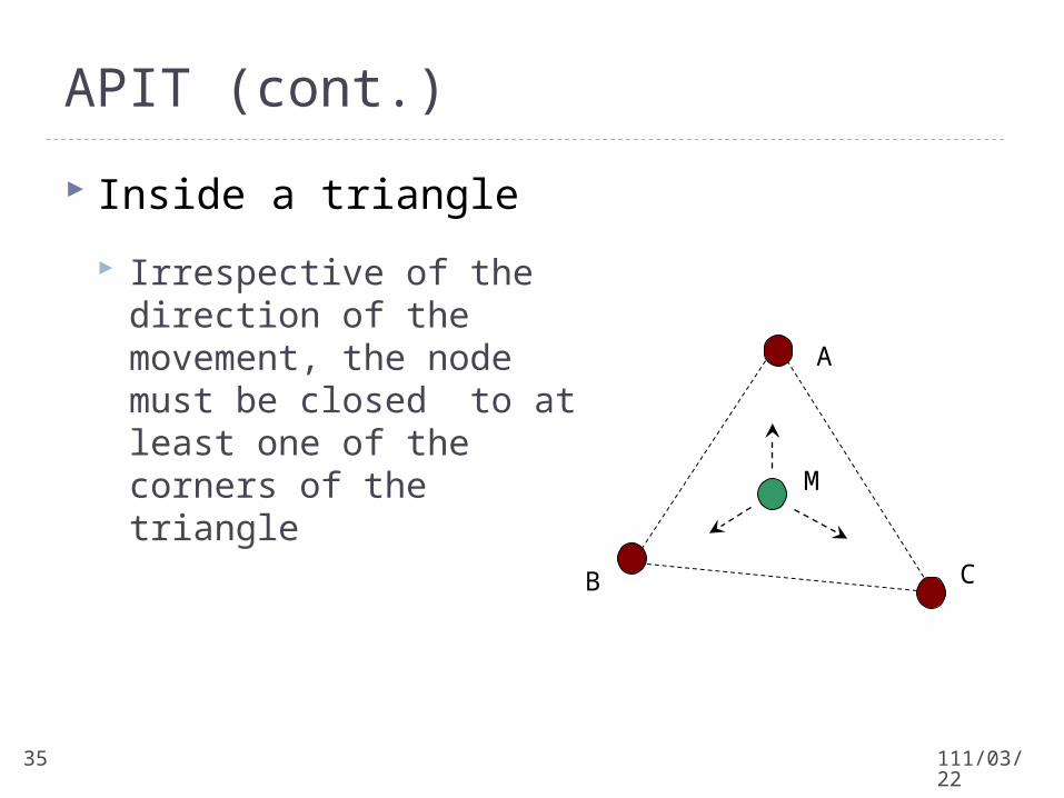
APIT (cont.)

Inside a triangle

Irrespective of the direction of the movement, the node must be closed to at least one of the corners of the triangle

A

CB

M

112/04/1935

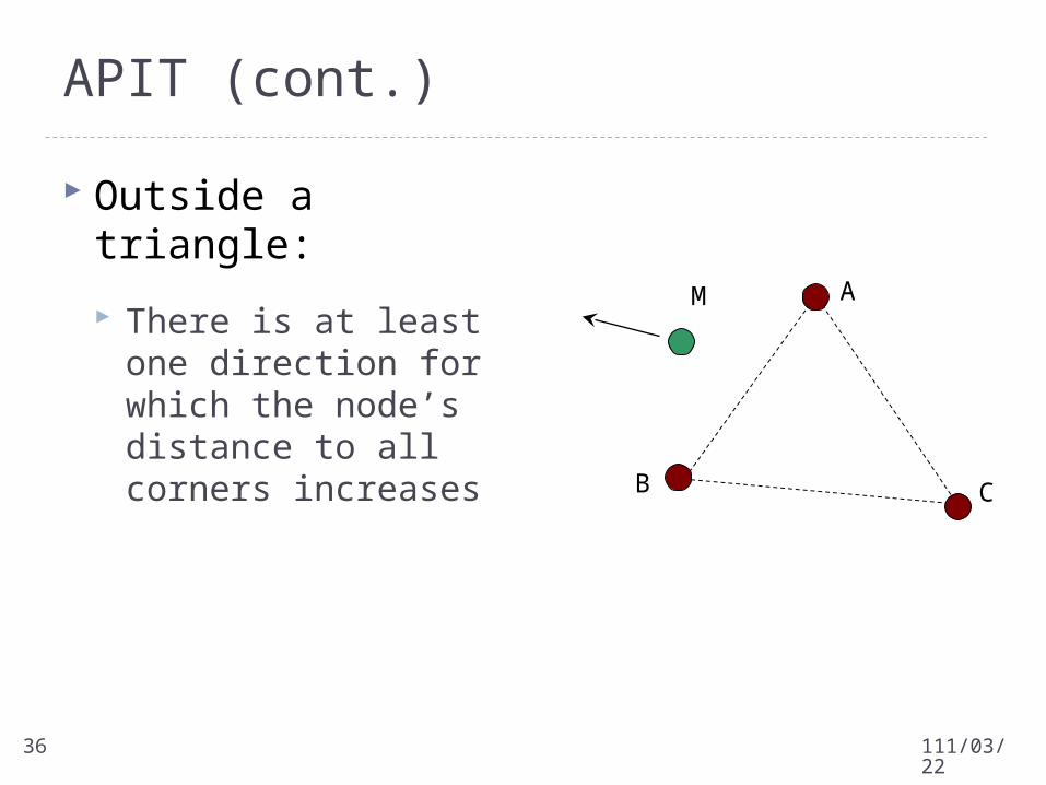
APIT (cont.)

Outside a triangle:

There is at least one direction for which the node’s distance to all corners increases

A

CB

M

112/04/1936

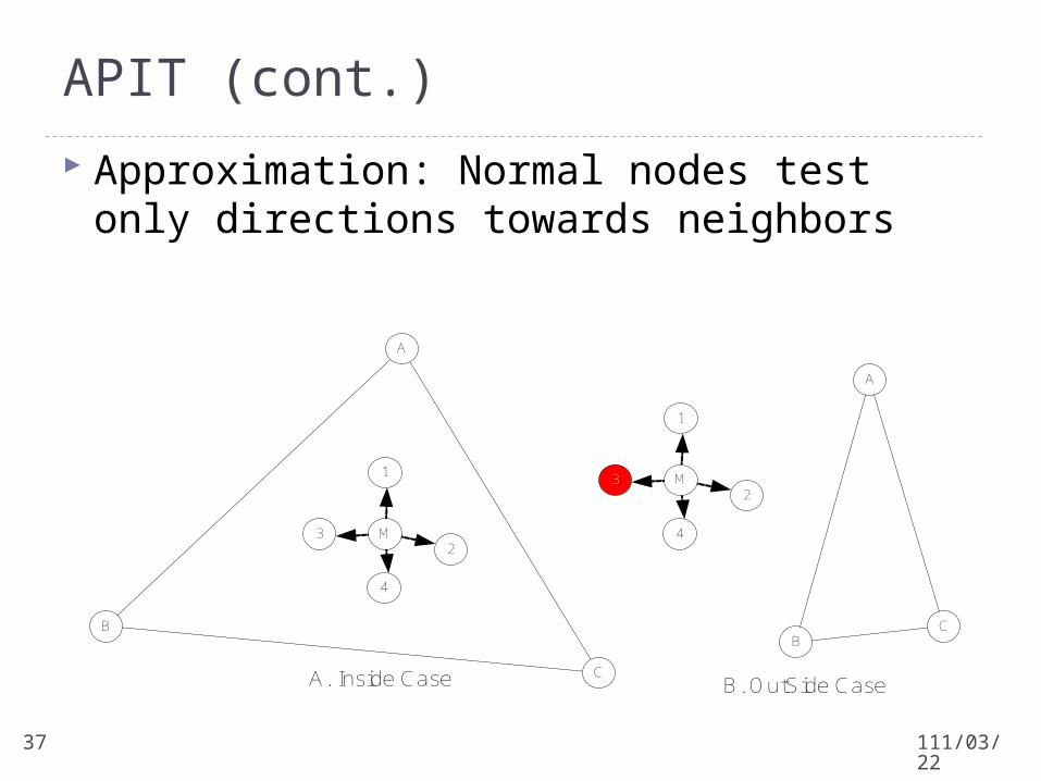
Approximation: Normal nodes test only directions towards neighbors

A

C

1

23

4

M

B

A

CB

A. Inside Case B. OutSide Case

1

23

4

M

APIT (cont.)

112/04/1937

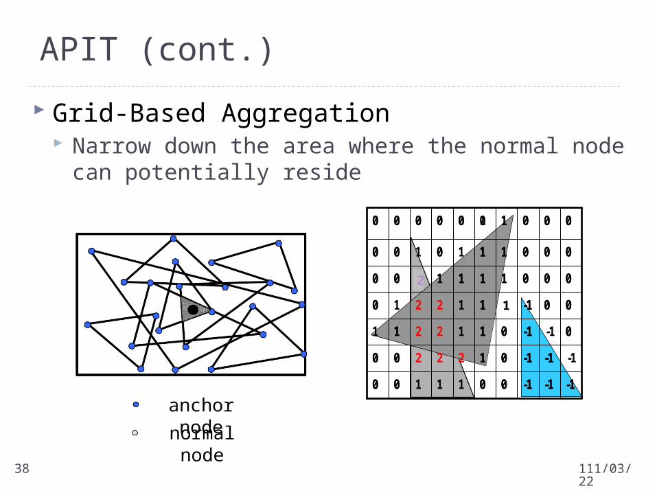
Grid-Based Aggregation Narrow down the area where the normal node can potentially

reside

-1-1-10011100

-1-1-10122200

0-1-10112211

00-10112210

0001111100

0001110100

0001000000

-1-1-10000

-1-10100

0-1011

00-1010

00011100

00011000

0001100000

anchor node

normal node

1

2

APIT (cont.)

112/04/1938

112/04/19 39

MCL (Monte-Carlo Localization)

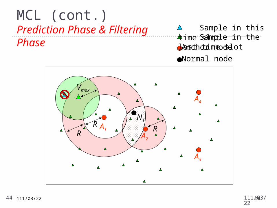
Assumptions Time is divided into several time slots Moving distance in each time slot is randomly chosen from

[0 , Vmax ] Each anchor node periodically forwards its location to two-

hop neighbors Notation

R - communication range

112/04/1939

112/04/19 40

MCL (cont.)

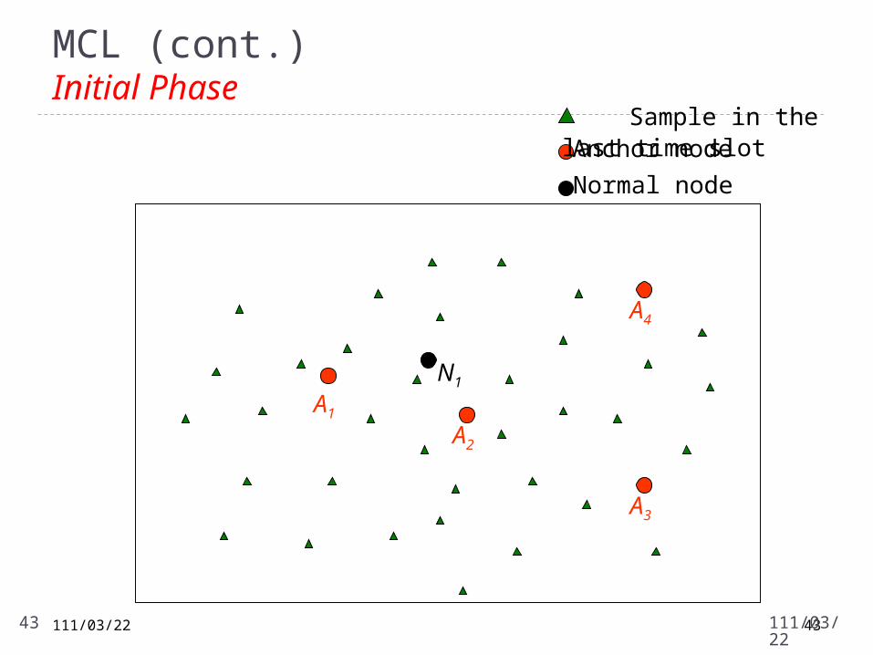
Each normal node maintains 50 samples in each time slot Samples represent the possible locations The sample selection is based on previous samples Sample (x , y) must satisfy some constraints

Located in the anchor constraints

112/04/1940

112/04/19 41

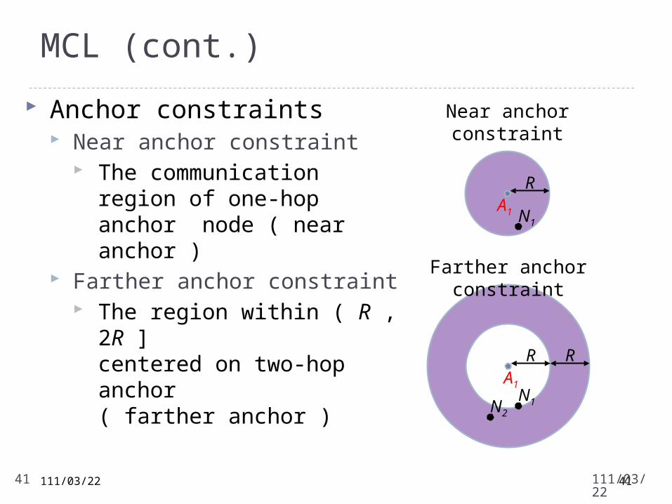
MCL (cont.)

Anchor constraints Near anchor constraint

The communication region of one-hop anchor node ( near anchor )

Farther anchor constraint The region within ( R , 2R ]

centered on two-hop anchor ( farther anchor )

Near anchor constraint

RA1

RR

Farther anchor constraint

A1

N1

N1N2

112/04/1941

112/04/19 42

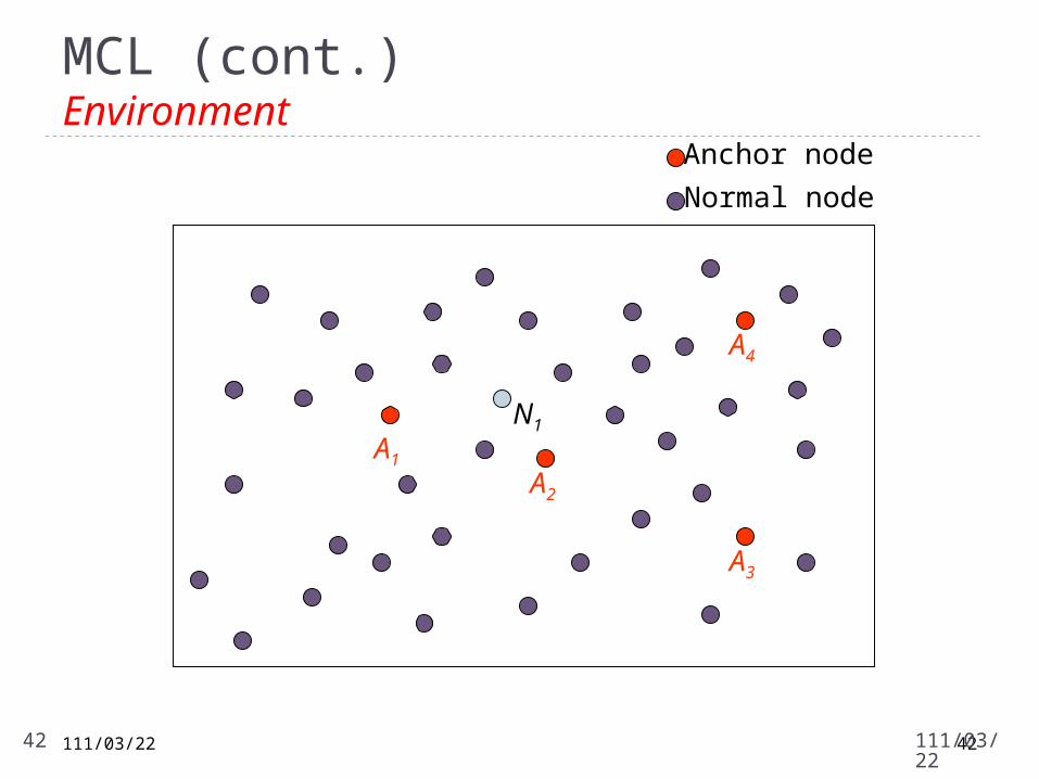
MCL (cont.)Environment

Anchor node

Normal node

A1

A2

A3

A4

N1

112/04/1942

112/04/19 43

MCL (cont.)Initial Phase

N1

A1

A2

A3

A4

Anchor node

Normal node

Sample in the last time slot

112/04/1943

112/04/19 44

RR

R

MCL (cont.)Prediction Phase & Filtering Phase

N1

A1

A2

A3

A4

Vmax

Anchor node

Normal node

Sample in the last time slot Sample in this time slot

112/04/1944

112/04/19 45

R

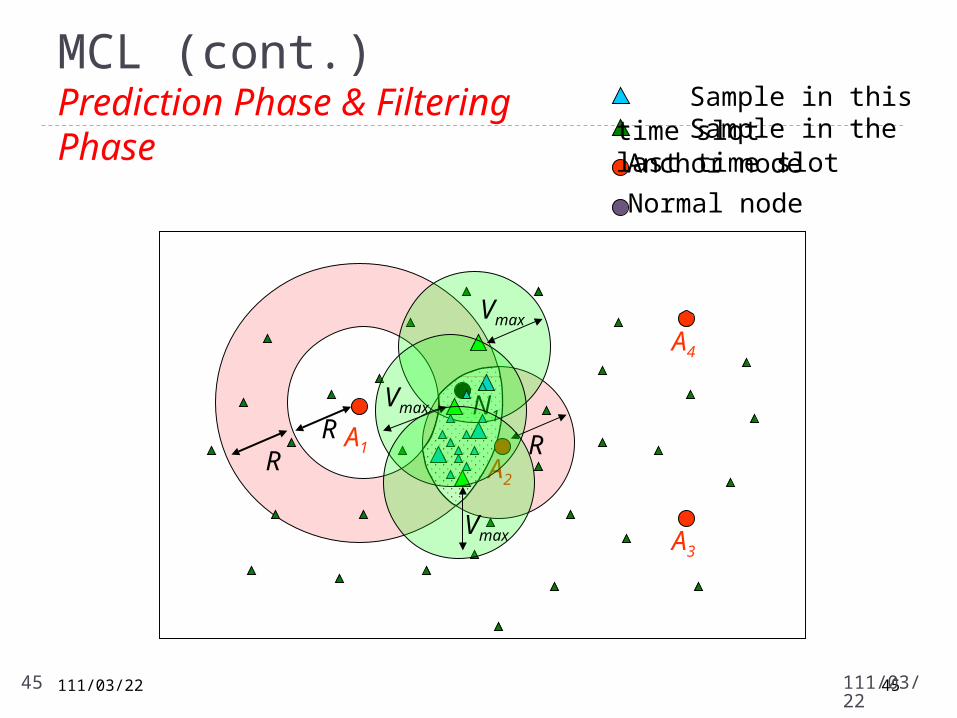
MCL (cont.)Prediction Phase & Filtering Phase

N1

A1

A2

A3

A4

Vmax

Vmax

Vmax

Anchor node

Normal node

RR

Sample in the last time slot Sample in this time slot

112/04/1945

112/04/19 46

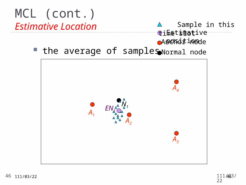
MCL (cont.)Estimative Location

N1

A1

A2

A3

A4

the average of samples

EN1

Anchor node

Normal node

Estimative position Sample in this time slot

112/04/1946

112/04/19 47

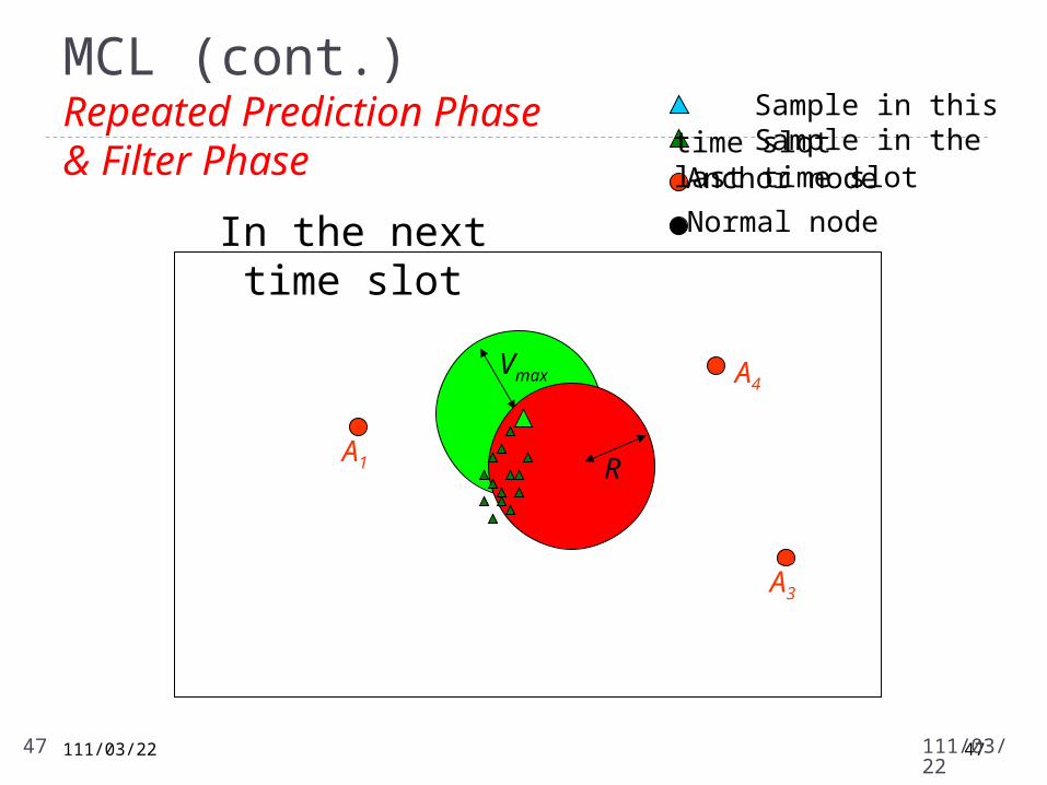
MCL (cont.) Repeated Prediction Phase & Filter Phase

Vmax

N1A1

A2

A3

A4

R

In the next time slot

Anchor node

Normal node

Sample in the last time slot Sample in this time slot

112/04/1947

There are three phases in the DRLS algorithm.

Phase 1 – Beacon exchange

Phase 2 – Using improved grid-scan algorithm to get initial estimative location

Phase 3 – Refinement

DRLS Distributed Range-Free Localization Scheme

112/04/1948

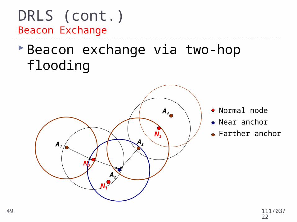
Beacon exchange via two-hop flooding

N1

Near anchor

Normal node

A1

A2

A3

A4

N2

N3 Farther anchor

DRLS (cont.)Beacon Exchange

112/04/1949

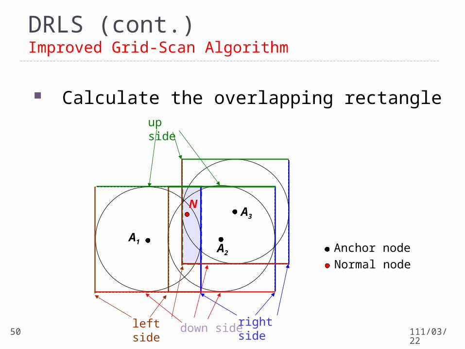
DRLS (cont.)Improved Grid-Scan Algorithm

A2

A3

A1

N

Normal node

Anchor node

right sideleft side

up side

down side

Calculate the overlapping rectangle

112/04/1950

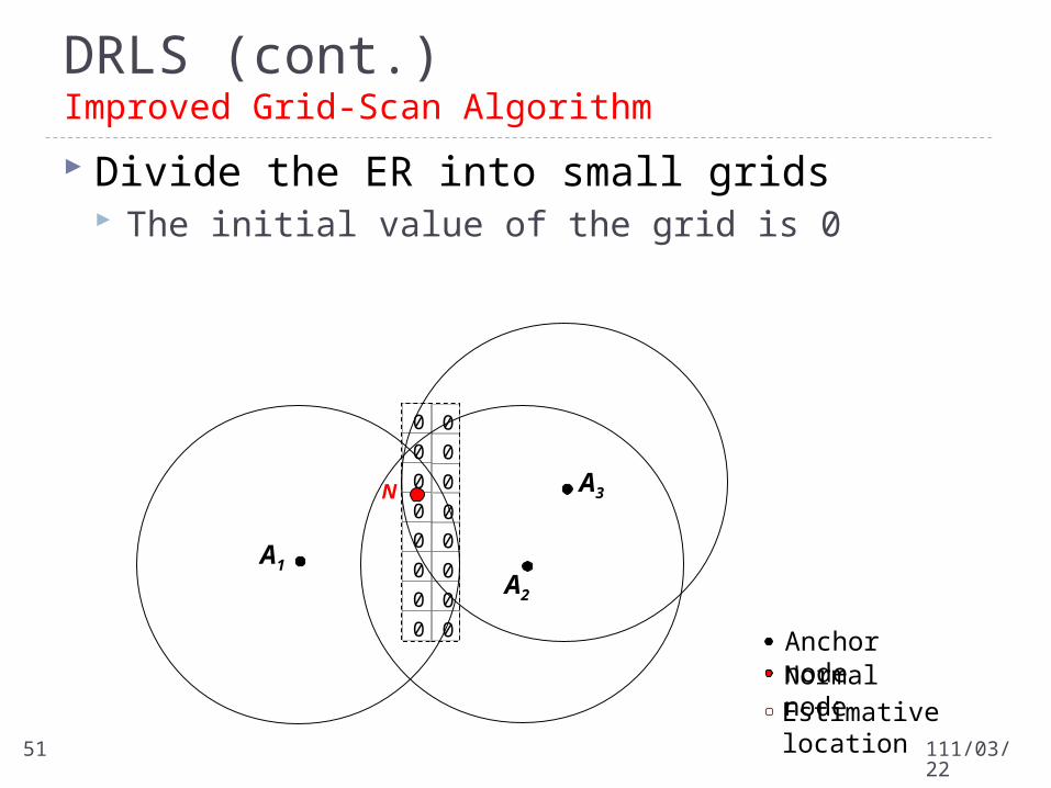
DRLS (cont.)Improved Grid-Scan Algorithm

Divide the ER into small grids The initial value of the grid is 0

0

0

0

0

00

0 0

0

A2

A3

A1

0 0

0

0

0

0

N

0

Anchor nodeNormal node

Estimative location112/04/1951

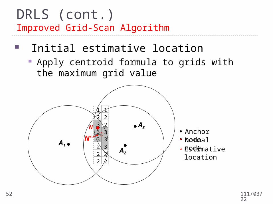
DRLS (cont.)Improved Grid-Scan Algorithm

2

2

2

3

333 3

3

A2

A3

A1

1 1

2

2

2

2

N

N’2

Anchor nodeNormal nodeEstimative location

Initial estimative location Apply centroid formula to grids with the maximum grid

value

112/04/1952

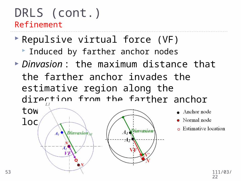
Repulsive virtual force (VF) Induced by farther anchor nodes

Dinvasion : the maximum distance that the farther anchor invades the estimative region along the direction from the farther anchor towards the initial estimative location

DRLS (cont.)Refinement

112/04/1953

VFA3

DinvasionA3

VFA4

DinvasionA4

VFA5

DinvasionA5

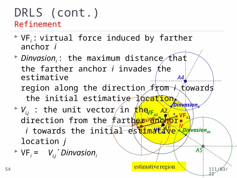
VFi : virtual force induced by farther anchor i Dinvasioni : the maximum distance that

the farther anchor i invades the estimative region along the direction from i towards the initial estimative location

Vi,j : the unit vector in the direction from the farther anchor i towards the initial estimative location j

VFi = Vi,j˙Dinvasioni

A4

A5

A1

A2

NN’A3

DRLS (cont.)Refinement

112/04/1954

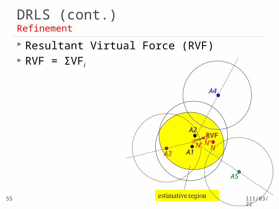
RVF

Resultant Virtual Force (RVF) RVF = ΣVFi

A4

A5

A1

A2

NN’A3

N’

DRLS (cont.)Refinement

112/04/1955

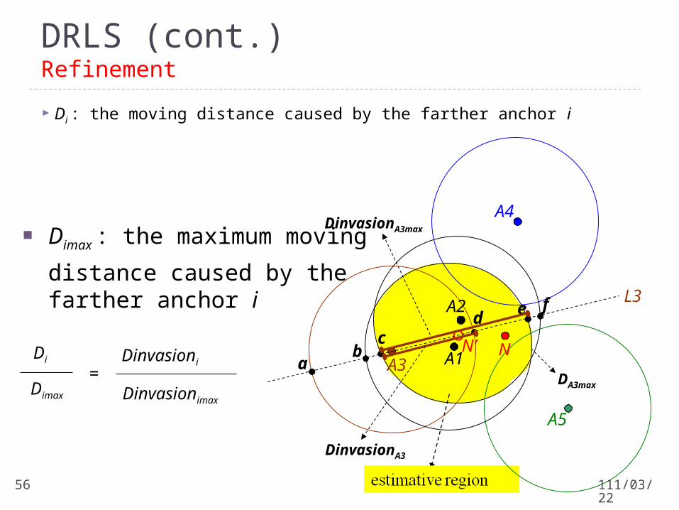
DA3max

Dimax : the maximum moving

distance caused by the farther anchor i

Di : the moving distance caused by the farther anchor i

A4

A5

A1

A2

NN’A3

L3

ab

cd

e f

DinvasionA3

Di

Dimax

=Dinvasioni

Dinvasionimax

DinvasionA3max

DRLS (cont.)Refinement

112/04/1956

Dmovei : the moving vector caused by the

farther anchor i Vi,j : the unit vector in the

direction from the farther anchor

i towards the initial estimative

location j Dmovei = Vi,j˙Di

estimative region

DmoveA3

DinvasionA3

DmoveA4

DinvasionA4

DmoveA5

DinvasionA5

A4

A5

A1

A2

NN’A3

DRLS (cont.)Refinement

112/04/1957

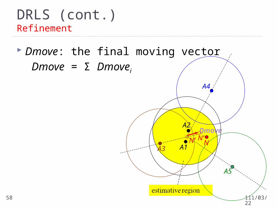
Dmove: the final moving vector

Dmove = Σ Dmovei

Dmove

A4

A5

A1

A2

NN’A3

N’

DRLS (cont.)Refinement

112/04/1958

Improvements Dynamic number of samples

According to the overlapping region of anchor constraints Restricted samples

Anchor constraints The estimative locations of neighboring normal nodes

Predicted moving direction of the normal node Be used to increase the localization accuracy

IMCL Improved MCL Localization Scheme

112/04/1959

Phase 1- Sample Selection Phase

Phase 2- Neighbor Constraints Exchange Phase

Phase 3- Refinement Phase

IMCL (cont.)

112/04/1960

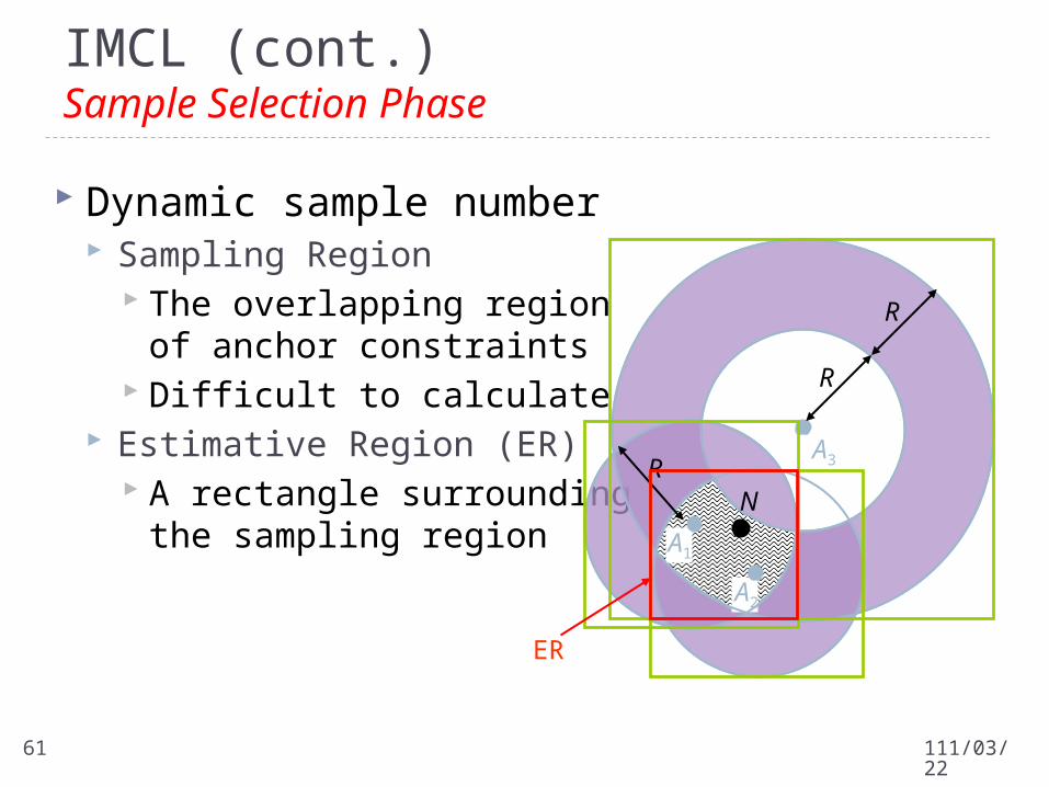
Dynamic sample number Sampling Region

The overlapping region of anchor constraints

Difficult to calculate Estimative Region (ER)

A rectangle surrounding the sampling region A1

A2

A3

R

R

R

ER

N

IMCL (cont.) Sample Selection Phase

112/04/1961

IMCL (cont.) Sample Selection Phase

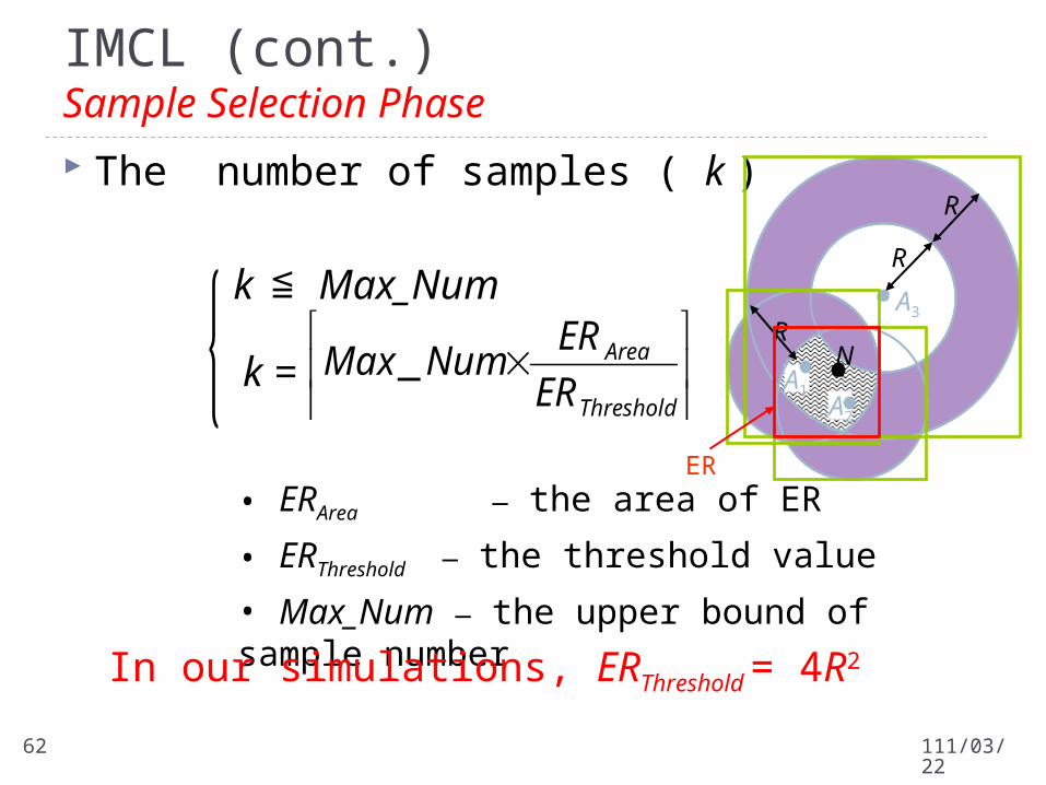
The number of samples ( k )

k =

• ERArea — the area of ER

• ERThreshold — the threshold value

• Max_Num — the upper bound of sample number

In our simulations, ERThreshold = 4R2

Threshold

Area

ER

ERNumMax _

k ≦ Max_Num

A1A2

A3

R

R

R

ER

N

112/04/1962

IMCL (cont.) Sample Selection Phase

Using the prediction and filtering phase of MCL Samples are randomly selected from the region

extended Vmax from previous samples Filter new samples

Near anchor constraints Farther anchor constraints

112/04/1963

N2

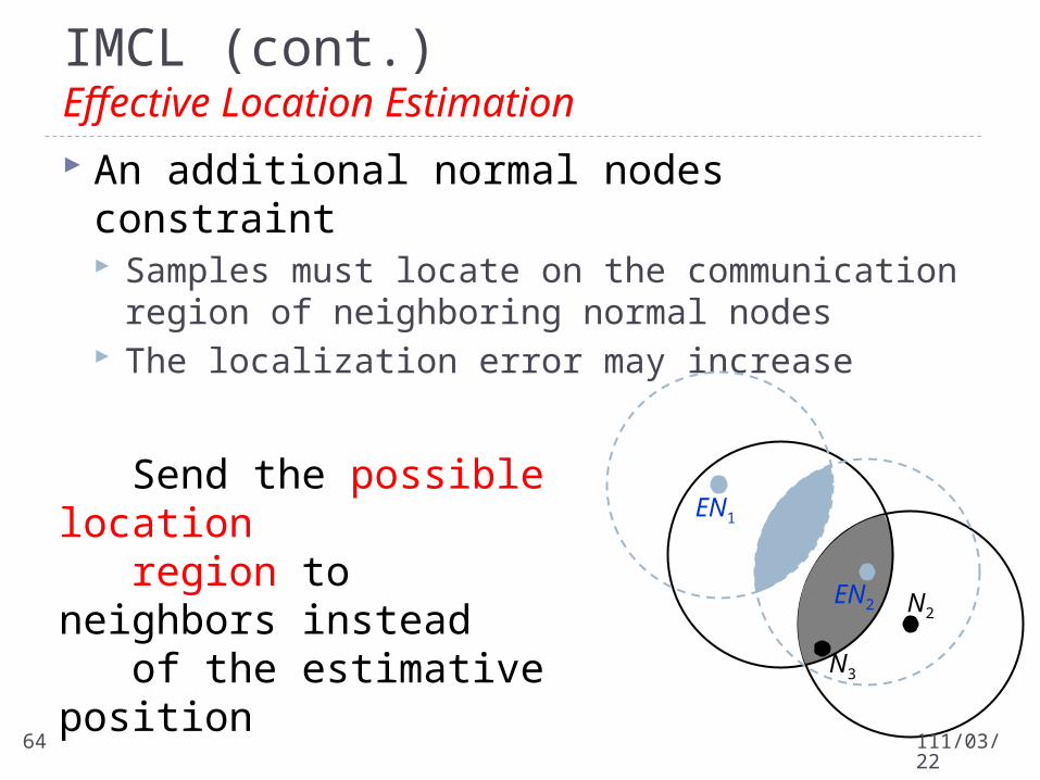
IMCL (cont.) Effective Location Estimation

An additional normal nodes constraint Samples must locate on the communication region of

neighboring normal nodes The localization error may increase

N1

N3

Send the possible location region to neighbors instead of the estimative position

EN1

EN2

112/04/1964

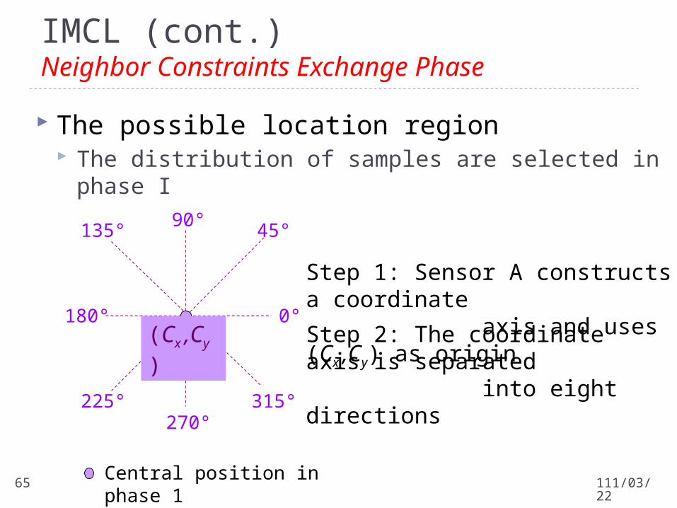
The possible location region The distribution of samples are selected in phase I

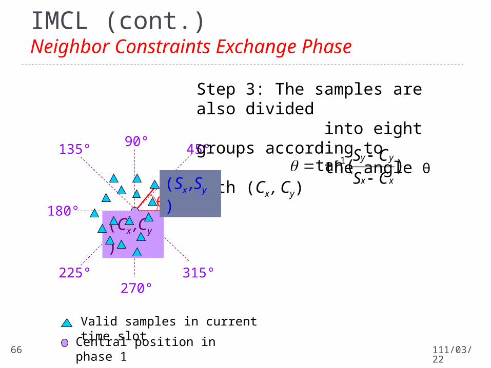
IMCL (cont.) Neighbor Constraints Exchange Phase

Step 1: Sensor A constructs a coordinate axis and uses (Cx ,Cy) as origin

Step 2: The coordinate axis is separated into eight directions

Central position in phase 1

45°135°

225° 315°

90°

270°

180° 0°(Cx ,Cy)

112/04/1965

θ

45°90°

135°

180° 0°

225°270°

315°

IMCL (cont.) Neighbor Constraints Exchange Phase

Step 3: The samples are also divided into eight groups according to the angle θ with (Cx , Cy)

(Cx ,Cy)

(Sx ,Sy))(tan 1

xx

yy

CS

CS

Valid samples in current time slot

Central position in phase 1112/04/1966

45°90°

135°

180° 0°

225°270°

315°

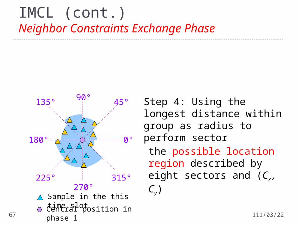
IMCL (cont.) Neighbor Constraints Exchange Phase

Step 4: Using the longest distance within group as radius to perform sector

the possible location region described by eight sectors and (Cx , Cy)

Sample in the this time slot

Central position in phase 1112/04/1967

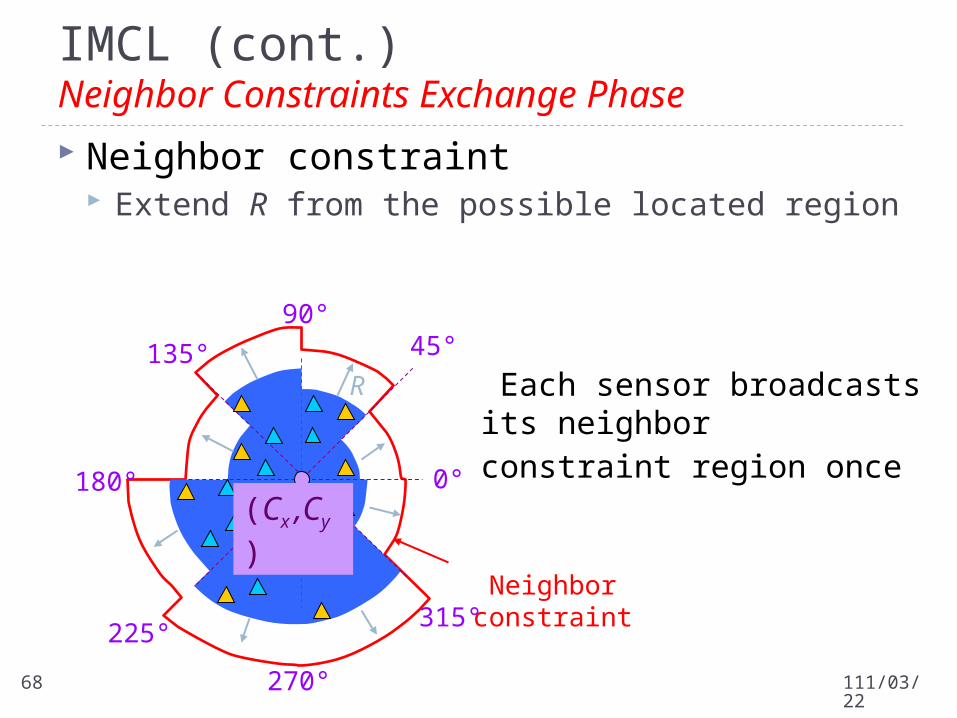
Neighbor constraint Extend R from the possible located region

Neighbor constraint

90°45°135°

180° 0°

225°

270°

315°

(Cx ,Cy)

R Each sensor broadcasts its neighbor constraint region once

IMCL (cont.) Neighbor Constraints Exchange Phase

112/04/1968

IMCL (cont.) Refinement Phase

Samples are filtered Neighbor constraints

Receive from neighboring normal nodes Moving constraint

Predict the possible moving direction When sample is not satisfy the constraints

Normal node generates a valid sample to replace it

112/04/1969

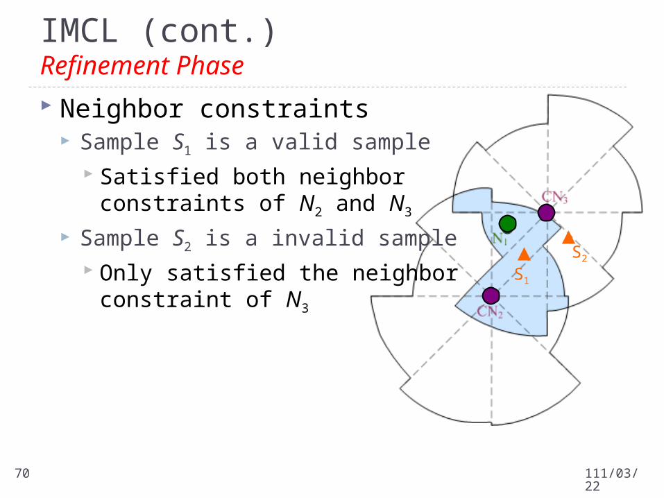
IMCL (cont.) Refinement Phase

S1

S2

Neighbor constraints Sample S1 is a valid sample

Satisfied both neighborconstraints of N2 and N3

Sample S2 is a invalid sample Only satisfied the neighbor

constraint of N3

112/04/1970

IMCL (cont.) Refinement Phase

Et-2

Et-1

θΔ Φ

Δ Φ(Cx , Cy)

(Cx , Cy)

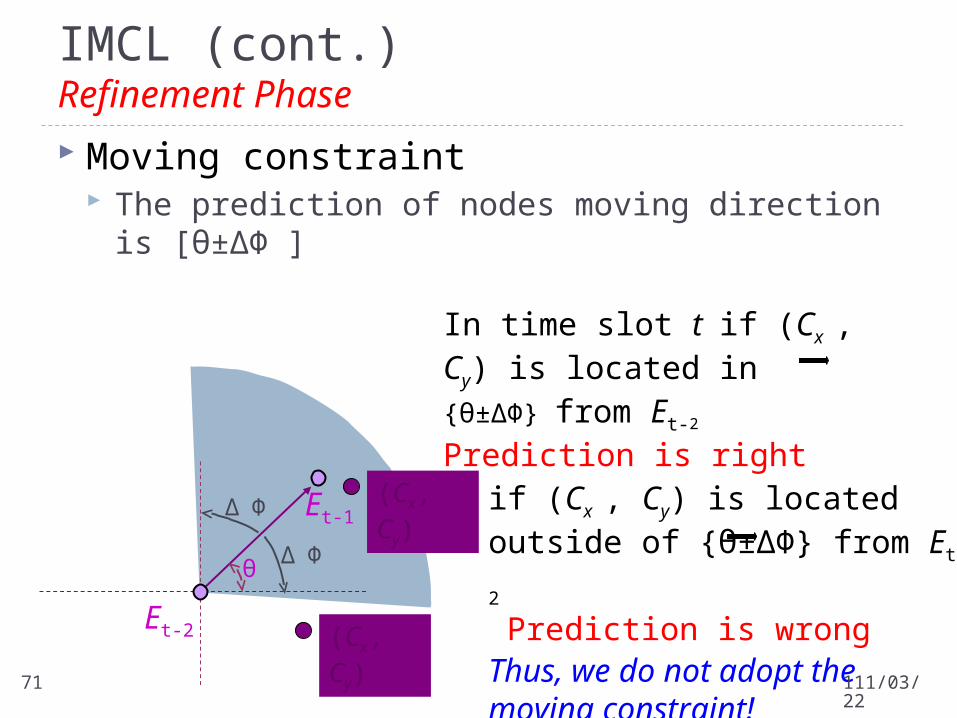
In time slot t if (Cx , Cy) is located in {θ±ΔΦ} from Et-2

Prediction is right

if (Cx , Cy) is located outside of {θ±ΔΦ} from Et-2

Prediction is wrongThus, we do not adopt the moving constraint!

Moving constraint The prediction of nodes moving direction is [θ±ΔΦ ]

112/04/1971

IMCL (cont.) Refinement Phase

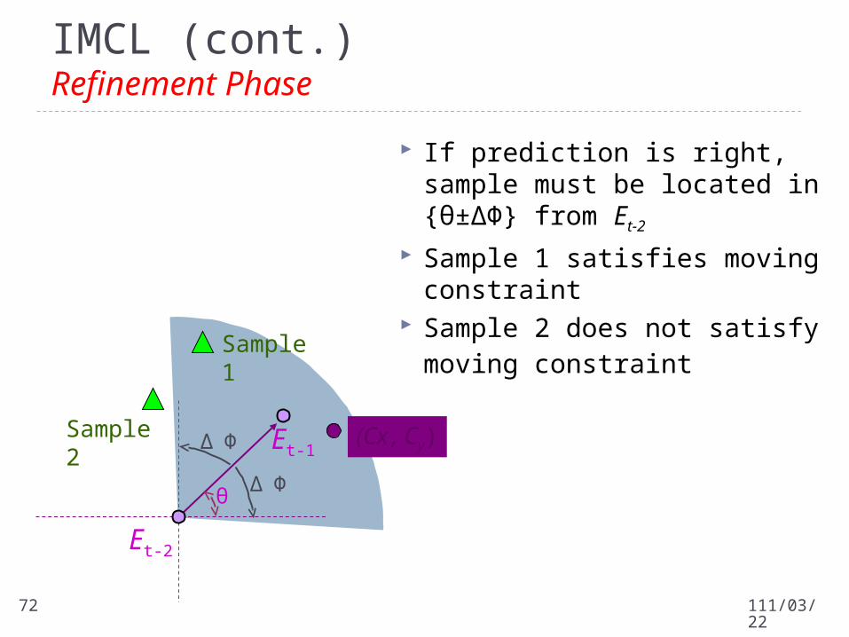
If prediction is right, sample must be located in {θ±ΔΦ} from Et-2

Sample 1 satisfies moving constraint

Sample 2 does not satisfy moving constraint

Et-2

Et-1

θΔ Φ

Δ Φ (Cx , Cy)

Sample 1

Sample 2

112/04/1972

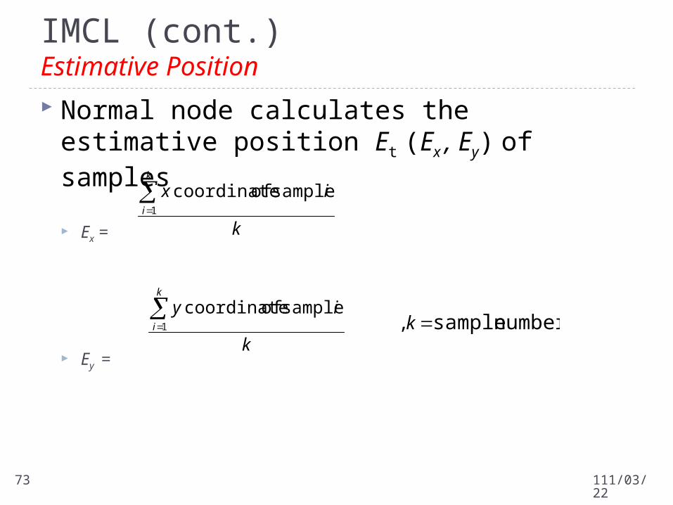
IMCL (cont.) Estimative Position

Normal node calculates the estimative position Et (Ex , Ey) of samples

Ex =

Ey =

k

ixk

i1

sample of coordinate

k

iyk

i1

sample of coordinate number sample , k

112/04/1973

Determining location or position is a really important function in WSN, but fraught with many errors and shortcomings

Range estimates often not sufficiently accurate Many anchors are needed for acceptable results Anchors might need external position sources (GPS)

Conclusions

112/04/1974

References J. Hightower and G. Borriello. “Location Systems for Ubiquitous Computing,”

IEEE Computer, 34(8): 57–66, 2001. J. Hightower and G. Borriello. “A Survey and Taxonomy of Location Systems for

Ubiquitous Computing,” Technical Report UW-CSE 01-08-03, University of Washington, Computer Science and Engineering, Seattle, WA, August 2001.

A. Boukerche, H. Oliveira, E. Nakamura, and A. Loureiro. “Localization systems for wireless sensor networks”. IEEE Wireless Communications, December 2007.

R. Want, A. Hopper, V. Fal˜ao, and J. Gibbons. The Active Badge Location System. ACM Transactions on Information Systems, 10(1): 91–102, 1992.

A. Ward, A. Jones, and A. Hopper. A New Location Technique for the Active Office. IEEE Personal Communications, 4(5): 42–47, 1997.

P. Bahl and V. N. Padmanabhan. RADAR: An In-Building RF-Based User Location and Tracking System. In Proceedings of the IEEE INFOCOM, pages 775–784, Tel-Aviv, Israel, April 2000.

N. B. Priyantha, A. Chakraborty, and H. Balakrishnan. The Cricket Location-Support System. In Proceedings of the 6th International Conference on Mobile Computing and Networking (ACM Mobicom), Boston, MA, 2000.

112/04/1975

References

N. Bulusu, J. Heidemann, and D. Estrin. “GPS-Less Low Cost Outdoor Localization For Very Small Devices,” IEEE Personal Communications Magazine, 7(5): 28–34, 2000.

C. Savarese, J. Rabay, and K. Langendoen. “Robust Positioning Algorithms for Distributed Ad-Hoc Wireless Sensor Networks,” In Proceedings of the Annual USENIX Technical Conference, Monterey, CA, 2002.

A. Savvides, C.-C. Han, and M. Srivastava. “Dynamic Fine-Grained Localization in Ad-Hoc Networks of Sensors,” Proceedings of the 7th Annual International Conference on Mobile Computing and Networking, pages 166–179. ACM press, Rome, Italy, July 2001.

S. Simic and S. Sastry, “Distributed localization in wireless ad hoc networks,” UC Berkeley, Tech. rep. UCB/ERL M02/26, 2002. D. Niculescu and B. Nath. “Ad Hoc Positioning System (APS)”. In Proceedings of IEEE GlobeCom, San Antonio, AZ, November 2001.

C. Savarese, J. M. Rabaey, and J. Beutel. “Locationing in Distributed Ad-Hoc Wireless Sensor Networks”. In Proceedings of the International Conference on Acoustics, Speech and Signal Processing (ICASSP 2001), Salt Lake City, Utah, May 2001.

112/04/1976

References V. Ramadurai and M. L. Sichitiu. “Localization in Wireless Sensor Networks: A

Probabilistic Approach”. In Proceedings of 2003 International Conference on Wireless Networks (ICWN 2003), pages 300–305, Las Vegas, NV, June 2003.

M. L. Sichitiu and V. Ramadurai, “Localization of Wireless Sensor Networks with A Mobile Beacon,” Proc. 1st IEEE Int’l. Conf. Mobile Ad Hoc and Sensor Sys., FL, Oct. 2004, pp. 174–83.

N.Bodhi Priyantha, H. Balakrishnan, E. Demaine, S. Teller,”Mobile-Assisted Localization in Sensor Network”, IEEE INFOCOM 2005, Miami, FL, March 2005.

T. He, C. Huang, B. M. Blum, J. A. Stankovic, and T. Abdelzaher. Range-Free Localization Schemes for Large Scale Sensor Networks. Proceedings of the 9th Annual International Conference on Mobile Computing and Networking, pages 81–95. ACM Press, 2003.

F. Dellaert, D. Fox, W. Burgard, and S. Thrun, "Monte Carlo Localization for Mobile Robots", IEEE International Conference on Robotics and Automation (ICRA), 1999

L. Hu and D. Evans, "Localization for Mobile Sensor Networks," Proc. ACM MobiCom, pp. 45-47, Sept. 2004.

112/04/1977

References J.-P. Sheu, P.-C. Chen, and C.-S. Hsu, “A Distributed Localization Scheme for

Wireless Sensor Networks with Improved Grid-Scan and Vector-Based Refinement,” IEEE Trans. on Mobile Computing, vol. 7, no. 9, pp. 1110-1123, Sept. 2008.

Jang-Ping Sheu, Wei-Kai Hu, and Jen-Chiao Lin, "Distributed Localization Scheme for Mobile Sensor Networks," IEEE Transactions on Mobile Computing Vol. 9, No. 4, pp. 516 - 526, April 2010.

112/04/1978