chapter 7: optimization of distributed queries

Chapter 7: Optimization of DistributedQueries

• Basic Concepts

• Distributed Cost Model

• Database Statistics

• Joins and Semijoins

• Query Optimization Algorithms

Acknowledgements: I am indebted to Arturas Mazeika for providing me his slides of this course.

DDB 2008/09 J. Gamper

Basic Concepts

• Query optimization: Process of producing an op-timal (close to optimal) query execution plan whichrepresents an execution strategy for the query

– The main task in query optimization is to con-sider different orderings of the operations

• Centralized query optimization:

– Find (the best) query execution plan in thespace of equivalent query trees

– Minimize an objective cost function

– Gather statistics about relations

• Distributed query optimization brings additional issues

– Linear query trees are not necessarily a good choice

– Bushy query trees are not necessarily a bad choice

– What and where to ship the relations

– How to ship relations (ship as a whole, ship as needed)

– When to use semi-joins instead of joins


Basic Concepts . . .

• Search space: The set of alternative query execution plans (query trees)

– Typically very large

– The main issue is to optimize the joins

– For N relations, there are O(N !) equivalent join trees that can be obtained byapplying commutativity and associativity rules

• Example : 3 equivalent query trees (join trees) of the joins in the following query

SELECT ENAME,RESPFROM EMP, ASG, PROJWHERE EMP.ENO=ASG.ENO AND ASG.PNO=PROJ.PNO



• Reduction of the search space

– Restrict by means of heuristics

∗ Perform unary operations before binary operations, etc

– Restrict the shape of the join tree

∗ Consider the type of trees (linear trees, vs. bushy ones)

Linear Join Tree Bushy Join Tree



• There are two main strategies to scan the search space

– Deterministic

– Randomized

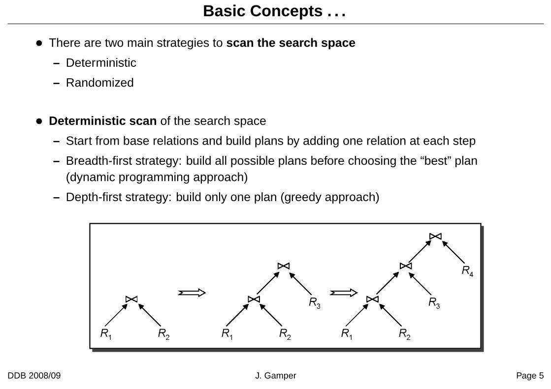
• Deterministic scan of the search space

– Start from base relations and build plans by adding one relation at each step

– Breadth-first strategy: build all possible plans before choosing the “best” plan(dynamic programming approach)

– Depth-first strategy: build only one plan (greedy approach)



• Randomized scan of the search space

– Search for optimal solutions around a particular starting point

– e.g., iterative improvement or simulated annealing techniques

– Trades optimization time for execution time

∗ Does not guarantee that the best solution is obtained, but avoid the high cost ofoptimization

– The strategy is better when more than 5-6 relations are involved


Distributed Cost Model

• Two different types of cost functions can be used

– Reduce total time

∗ Reduce each cost component (in terms of time) individually, i.e., do as little for eachcost component as possible

∗ Optimize the utilization of the resources (i.e., increase system throughput)

– Reduce response time

∗ Do as many things in parallel as possible∗ May increase total time because of increased total activity


Distributed Cost Model . . .

• Total time : Sum of the time of all individual components

– Local processing time: CPU time + I/O time

– Communication time: fixed time to initiate a message + time to transmit the data

Total time =TCPU ∗ #instructions + TI/O ∗ #I /Os +

TMSG ∗ #messages + TTR ∗ #bytes

• The individual components of the total cost have different weights:

– Wide area network

∗ Message initiation and transmission costs are high∗ Local processing cost is low (fast mainframes or minicomputers)∗ Ratio of communication to I/O costs is 20:1

– Local area networks

∗ Communication and local processing costs are more or less equal∗ Ratio of communication to I/O costs is 1:1.6 (10MB/s network)



• Response time : Elapsed time between the initiation and the completion of a query

Response time =TCPU ∗ #seq instructions + TI/O ∗ #seq I /Os +

TMSG ∗ #seq messages + TTR ∗ #seq bytes

– where #seq x (x in instructions, I/O, messages, bytes) is the maximum number ofx which must be done sequentially.

• Any processing and communication done in parallel is ignored



• Example: Query at site 3 with data from sites 1 and 2.

– Assume that only the communication cost is considered

– Total time = TMSG ∗ 2 + TTR ∗ (x + y)

– Response time = max{TMSG + TTR ∗ x, TMSG + TTR ∗ y}


Database Statistics

• The primary cost factor is the size of intermediate relations

– that are produced during the execution and

– must be transmitted over the network, if a subsequent operation is located on adifferent site

• It is costly to compute the size of the intermediate relations precisely.

• Instead global statistics of relations and fragments are computed and used toprovide approximations


Database Statistics . . .

• Let R(A1, A2, . . . , Ak) be a relation fragmented into R1, R2, . . . , Rr.

• Relation statistics

– min and max values of each attribute: min{Ai}, max{Ai}.

– length of each attribute: length(Ai)

– number of distinct values in each fragment (cardinality): card(Ai),(card(dom(Ai)))

• Fragment statistics

– cardinality of the fragment: card(Ri)

– cardinality of each attribute of each fragment: card(ΠAi(Rj))



• Selectivity factor of an operation: the proportion of tuples of an operand relation thatparticipate in the result of that operation

• Assumption: independent attributes and uniform distribution of attribute values

• Selectivity factor of selection

SFσ(A = value) =1

card(ΠA(R))

SFσ(A > value) =max(A) − value

max(A) − min(A)

SFσ(A < value) =value − min(A)

max(A) − min(A)

• Properties of the selectivity factor of the selection

SFσ(p(Ai) ∧ p(Aj)) = SFσ(p(Ai)) ∗ SFσ(p(Aj))

SFσ(p(Ai) ∨ p(Aj)) = SFσ(p(Ai)) + SFσ(p(Aj)) − (SFσ(p(Ai)) ∗ SFσ(p(Aj))

SFσ(A ∈ {values}) = SFσ(A = value) ∗ card({values})



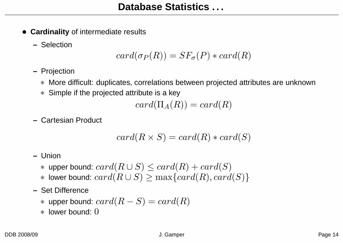
• Cardinality of intermediate results

– Selection

card(σP (R)) = SFσ(P ) ∗ card(R)

– Projection

∗ More difficult: duplicates, correlations between projected attributes are unknown∗ Simple if the projected attribute is a key

card(ΠA(R)) = card(R)

– Cartesian Product

card(R × S) = card(R) ∗ card(S)

– Union

∗ upper bound: card(R ∪ S) ≤ card(R) + card(S)∗ lower bound: card(R ∪ S) ≥ max{card(R), card(S)}

– Set Difference

∗ upper bound: card(R − S) = card(R)∗ lower bound: 0



• Selectivity factor for joins

SF⋊⋉ =card(R ⋊⋉ S)

card(R) ∗ card(S)

• Cardinality of joins

– Upper bound: cardinality of Cartesian Productcard(R ⋊⋉ S) ≤ card(R) ∗ card(S)

– General case (if SF is given):

card(R ⋊⋉ S) = SF⋊⋉ ∗ card(R) ∗ card(S)

– Special case: R.A is a key of R and S.A is a foreign key of S;

∗ each S-tuple matches with at most one tuple of R

card(R ⋊⋉R.A=S.A S) = card(S)



• Selectivity factor for semijoins: fraction of R-tuples that join with S-tuples

– An approximation is the selectivity of A in S

SF⊲<(R ⊲<A S) = SF⊲<(S.A) =card(ΠA(S))

card(dom[A])

• Cardinality of semijoin (general case):

card(R⊲<A S) = SF⊲<(S.A) ∗ card(R)

• Example: R.A is a foreign key in S (S.A is a primary key)Then SF = 1 and the result size corresponds to the size of R


Join Ordering in Fragment Queries

• Join ordering is an important aspect in centralized DBMS, and it is even moreimportant in a DDBMS since joins between fragments that are stored at different sitesmay increase the communication time.

• Two approaches exist:

– Optimize the ordering of joins directly

∗ INGRES and distributed INGRES∗ System R and System R∗

– Replace joins by combinations of semijoins in order to minimize the communicationcosts

∗ Hill Climbing and SDD-1


Join Ordering in Fragment Queries . . .

• Direct join odering of two relation/fragments located at different sites

– Move the smaller relation to the other site

– We have to estimate the size of R and S



• Direct join ordering of queries involving more than two relations is substantially morecomplex

• Example: Consider the following query and the respective join graph, where we makealso assumptions about the locations of the three relations/fragments

PROJ ⋊⋉PNO ASG ⋊⋉ENO EMP



• Example (contd.): The query can be evaluated in at least 5 different ways.

– Plan 1: EMP→Site 2

Site 2: EMP’=EMP⋊⋉ASG

EMP’→Site 3

Site 3: EMP’⋊⋉PROJ

– Plan 2: ASG→Site 1

Site 1: EMP’=EMP⋊⋉ASG

EMP’→Site 3

Site 3: EMP’⋊⋉PROJ

– Plan 3: ASG→Site 3

Site 3: ASG’=ASG⋊⋉PROJ

ASG’→Site 1

Site 1: ASG’⋊⋉EMP

– Plan 4: PROJ→Site 2

Site 2: PROJ’=PROJ⋊⋉ASG

PROJ’→Site 1

Site 1: PROJ’⋊⋉EMP

– Plan 5: EMP→Site 2

PROJ→Site 2

Site 2: EMP⋊⋉PROJ⋊⋉ASG

• To select a plan, a lot of information is needed, including

– size(EMP ), size(ASG), size(PROJ), size(EMP ⋊⋉ ASG),

size(ASG ⋊⋉ PROJ)

– Possibilities of parallel execution if response time is used


Semijoin Based Algorithms

• Semijoins can be used to efficiently implement joins

– The semijoin acts as a size reducer (similar as to a selection) such that smallerrelations need to be transferred

• Consider two relations: R located at site 1 and S located and site 2

– Solution with semijoins: Replace one or both operand relations/fragments by asemijoin, using the following rules:

R ⋊⋉A S ⇐⇒ (R ⊲<A S) ⋊⋉A S

⇐⇒ R ⋊⋉A (S ⊲<A R)

⇐⇒ (R ⊲<A S) ⋊⋉A (S ⊲<A R)

• The semijoin is beneficial if the cost to produce and send it to the other site is less thanthe cost of sending the whole operand relation and of doing the actual join.


Semijoin Based Algorithms

• Cost analysis R ⋊⋉A S vs. (R ⊲<A S) ⋊⋉ S, assuming that size(R) < size(S)

– Perform the join R ⋊⋉ S:

∗ R → Site 2∗ Site 2 computes R ⋊⋉ S

– Perform the semijoins (R ⊲< S) ⋊⋉ S:

∗ S′ = ΠA(S)∗ S′ →Site 1∗ Site 1 computes R′ = R ⊲< S′

∗ R′ →Site 2∗ Site 2 computes R′

⋊⋉ S

– Semijoin is better if: size(ΠA(S)) + size(R ⊲< S) < size(R)

• The semijoin approach is better if the semijoin acts as a sufficient reducer (i.e., a fewtuples of R participate in the join)

• The join approach is better if almost all tuples of R participate in the join


INGRES Algorithm

• INGRES uses a dynamic query optimization algorithm that recursively breaks a queryinto smaller pieces. It is based on the following ideas:

– An n-relation query q is decomposed into n subqueries q1 → q2 → · · · → qn

∗ Each qi is a mono-relation (mono-variable) query∗ The output of qi is consumed by qi+1

– For the decomposition two basic techniques are used: detachment and substitution

– There’s a processor that can efficiently process mono-relation queries

∗ Optimizes each query independently for the access to a single relation


INGRES Algorithm . . .

• Detachment: Break a query q into q′ → q′′, based on a common relation that is theresult of q′, i.e.

– The query

q: SELECT R2.A2, . . . , Rn.An

FROM R1, R2, . . . , Rn

WHERE P1(R1.A′

1)AND P2(R1.A1, . . . , Rn.An)

– is decomposed by detachment of the common relation R1 into

q′: SELECT R1.A1 INTO R′

1

FROM R1

WHERE P1(R1.A′

1)

q′′: SELECT R2.A2, . . . , Rn.An

FROM R′

1, R2, . . . , Rn

WHERE P2(R′

1.A1, . . . , Rn.An)

• Detachment reduces the size of the relation on which the query q′′ is defined.



• Example: Consider query q1: “Names of employees working on the CAD/CAM project”

q1: SELECT EMP.ENAMEFROM EMP, ASG, PROJWHERE EMP.ENO = ASG.ENOAND ASG.PNO = PROJ.PNOAND PROJ.PNAME = ”CAD/CAM”

• Decompose q1 into q11 → q′:

q11: SELECT PROJ.PNO INTO JVARFROM PROJWHERE PROJ.PNAME = ”CAD/CAM”

q′: SELECT EMP.ENAMEFROM EMP, ASG, JVARWHERE EMP.ENO = ASG.ENOAND ASG.PNO = JVAR.PNO



• Example (contd.): The successive detachments may transform q′ into q12 → q13:

q′: SELECT EMP.ENAMEFROM EMP, ASG, JVARWHERE EMP.ENO = ASG.ENOAND ASG.PNO = JVAR.PNO

q12: SELECT ASG.ENO INTO GVARFROM ASG,JVARWHERE ASG.PNO=JVAR.PNO

q13: SELECT EMP.ENAMEFROM EMP,GVARWHERE EMP.ENO=GVAR.ENO

• q1 is now decomposed by detachment into q11 → q12 → q13

• q11 is a mono-relation query

• q12 and q13 are multi-relation queries, which cannot be further detached.

– also called irreducible



• Tuple substitution allows to convert an irreducible query q into mono-relation queries.

– Choose a relation R1 in q for tuple substitution

– For each tuple in R1, replace the R1-attributes referred in q by their actual values,thereby generating a set of subqueries q′ with n − 1 relations, i.e.,

q(R1, R2, . . . , Rn) is replaced by {q′(t1i , R2, . . . , Rn), t1i ∈ R1}

• Example (contd.): Assume GVAR consists only of the tuples {E1, E2}. Then q13 isrewritten with tuple substitution in the following way

q13: SELECT EMP.ENAMEFROM EMP, GVARWHERE EMP.ENO = GVAR.ENO

q131: SELECT EMP.ENAMEFROM EMPWHERE EMP.ENO = ”E1”

q132: SELECT EMP.ENAMEFROM EMPWHERE EMP.ENO = ”E2”

– q131 and q132 are mono-relation queries


Distributed INGRES Algorithm

• The distributed INGRES query optimization algorithm is very similar to thecentralized INGRES algorithm.

– In addition to the centralized INGRES, the distributed one should break up eachquery qi into sub-queries that operate on fragments; only horizontal fragmentation ishandled.

– Optimization with respect to a combination of communication cost and response time


System R Algorithm

• The System R (centralized) query optimization algorithm

– Performs static query optimization based on “exhaustive search” of the solution spaceand a cost function (IO cost + CPU cost)

∗ Input: relational algebra tree∗ Output: optimal relational algebra tree∗ Dynamic programming technique is applied to reduce the number of alternative

plans

– The optimization algorithm consists of two steps

1. Predict the best access method to each individual relation (mono-relation query)∗ Consider using index, file scan, etc.

2. For each relation R, estimate the best join ordering∗ R is first accessed using its best single-relation access method∗ Efficient access to inner relation is crucial

– Considers two different join strategies

∗ (Indexed-) nested loop join∗ Sort-merge join


System R Algorithm . . .

• Example: Consider query q1: “Names of employees working on the CAD/CAM project”

PROJ ⋊⋉PNO ASG ⋊⋉ENO EMP

– Join graph

– Indexes

∗ EMP has an index on ENO∗ ASG has an index on PNO∗ PROJ has an index on PNO and an index on PNAME



• Example (contd.): Step 1 – Select the best single-relation access paths

– EMP: sequential scan (because there is no selection on EMP)

– ASG: sequential scan (because there is no selection on ASG)

– PROJ: index on PNAME (because there is a selection on PROJ based on PNAME)



• Example (contd.): Step 2 – Select the best join ordering for each relation

– (EMP × PROJ) and (PROJ × EMP) are pruned because they are CPs

– (ASG × PROJ) pruned because we assume it has higher cost than (PROJ × ASG);similar for (PROJ × EMP)

– Best total join order ((PROJ⋊⋉ ASG)⋊⋉ EMP), since it uses the indexes best

∗ Select PROJ using index on PNAME∗ Join with ASG using index on PNO∗ Join with EMP using index on ENO


Distributed System R∗ Algorithm

• The System R∗ query optimization algorithm is an extension of the System R queryoptimization algorithm with the following main characteristics:

– Only the whole relations can be distributed, i.e., fragmentation and replication is notconsidered

– Query compilation is a distributed task, coordinated by a master site , where thequery is initiated

– Master site makes all inter-site decisions, e.g., selection of the execution sites, joinordering, method of data transfer, ...

– The local sites do the intra-site (local) optimizations, e.g., local joins, access paths

• Join ordering and data transfer between different sites are the most critical issues to beconsidered by the master site


Distributed System R∗ Algorithm . . .

• Two methods for inter-site data transfer

– Ship whole: The entire relation is shipped to the join site and stored in a temporaryrelation

∗ Larger data transfer∗ Smaller number of messages∗ Better if relations are small

– Fetch as needed: The external relation is sequentially scanned, and for each tuplethe join value is sent to the site of the inner relation and the matching inner tuples aresent back (i.e., semijoin)

∗ Number of messages = O(cardinality of outer relation)∗ Data transfer per message is minimal∗ Better if relations are large and the selectivity is good



• Four main join strategies for R ⋊⋉ S:

– R is outer relation

– S is inner relation

• Notation:

– LT denotes local processing time

– CT denotes communication time

– s denotes the average number of S-tuples that match an R-tuple

• Strategy 1: Ship the entire outer relation to the site of the inner relation, i.e.,

– Retrieve outer tuples

– Send them to the inner relation site

– Join them as they arrive

Total cost = LT (retrieve card(R) tuples from R) +

CT (size(R)) +

LT (retrieve s tuples from S) ∗ card(R)



• Strategy 2: Ship the entire inner relation to the site of the outer relation. We cannot joinas they arrive; they need to be stored.

– The inner relation S need to be stored in a temporary relation

Total cost = LT (retrieve card(S) tuples from S) +

CT (size(S)) +

LT (store card(S) tuples in T ) +

LT (retrieve card(R) tuples from R) +

LT (retrieve s tuples from T ) ∗ card(R)



• Strategy 3: Fetch tuples of the inner relation as needed for each tuple of the outerrelation.

– For each R-tuple, the join attribute A is sent to the site of S

– The s matching S-tuples are retrieved and sent to the site of R

Total cost = LT (retrieve card(R) tuples from R) +

CT (length(A)) ∗ card(R) +

LT (retrieve s tuples from S) ∗ card(R) +

CT (s ∗ length(S)) ∗ card(R)



• Strategy 4: Move both relations to a third site and compute the join there.

– The inner relation S is first moved to a third site and stored in a temporary relation.

– Then the outer relation is moved to the third site and its tuples are joined as theyarrive.

Total cost = LT (retrieve card(S) tuples from S) +

CT (size(S)) +

LT (store card(S) tuples in T ) +

LT (retrieve card(R) tuples from R) +

CT (size(R)) +

LT (retrieve s tuples from T ) ∗ card(R)


Hill-Climbing Algorithm

• Hill-Climbing query optimization algorithm

– Refinements of an initial feasible solution are recursively computed until no more costimprovements can be made

– Semijoins, data replication, and fragmentation are not used

– Devised for wide area point-to-point networks

– The first distributed query processing algorithm


Hill-Climbing Algorithm . . .

• The hill-climbing algorithm proceeds as follows

1. Select initial feasible execution strategy ES0

– i.e., a global execution schedule that includes all intersite communication– Determine the candidate result sites, where a relation referenced in the query exist– Compute the cost of transferring all the other referenced relations to each

candidate site– ES0 = candidate site with minimum cost

2. Split ES0 into two strategies: ES1 followed by ES2

– ES1: send one of the relations involved in the join to the other relation’s site– ES2: send the join result to the final result site

3. Replace ES0 with the split schedule which gives

cost(ES1) + cost(local join) + cost(ES2) < cost(ES0)

4. Recursively apply steps 2 and 3 on ES1 and ES2 until no more benefit can be gained

5. Check for redundant transmissions in the final plan and eliminate them



• Example: What are the salaries of engineers who work on the CAD/CAM project?

ΠSAL(PAY ⋊⋉TITLE EMP ⋊⋉ENO (ASG ⋊⋉PNO (σPNAME=“CAD/CAM′′(PROJ))))

– Schemas: EMP(ENO, ENBAME, TITLE), ASG(ENO, PNO, RESP, DUR),

PROJ(PNO, PNAME, BUDGET, LOC), PAY(TITLE, SAL)

– Statistics

Relation Size Site

EMP 8 1

PAY 4 2

PROJ 1 3

ASG 10 4

– Assumptions:∗ Size of relations is defined as their cardinality∗ Minimize total cost∗ Transmission cost between two sites is 1∗ Ignore local processing cost∗ size(EMP ⋊⋉ PAY) = 8, size(PROJ ⋊⋉ ASG) = 2, size(ASG ⋊⋉ EMP) = 10



• Example (contd.): Determine initial feasible execution strategy

– Alternative 1: Resulting site is site 1

Total cost = cost(PAY → Site1) + cost(ASG → Site1) + cost(PROJ → Site1)

= 4 + 10 + 1 = 15


Total cost = 8 + 10 + 1 = 19


Total cost = 8 + 4 + 10 = 22


Total cost = 8 + 4 + 1 = 13

– Therefore ES0 = EMP→Site4; PAY → Site4; PROJ → Site4



• Example (contd.): Candidate split

– Alternative 1: ES1, ES2, ES3

∗ ES1: EMP→Site 2

∗ ES2: (EMP⋊⋉PAY) → Site4

∗ ES3: PROJ→Site 4

Total cost = cost(EMP → Site2) +

cost((EMP ⋊⋉ PAY) → Site4) +

cost(PROJ → Site4)

= 8 + 8 + 1 = 17

– Alternative 2: ES1, ES2, ES3

∗ ES1: PAY → Site1

∗ ES2: (PAY ⋊⋉ EMP) → Site4

∗ ES3: PROJ → Site 4

Total cost = cost(PAYSite → 1) +

cost((PAY ⋊⋉ EMP) → Site4) +

cost(PROJ → Site4)

= 4 + 8 + 1 = 13

• Both alternatives are not better than ES0, so keep it (or take alternative 2 which has thesame cost)



• Problems

– Greedy algorithm determines an initial feasible solution and iteratively improves it

– If there are local minima, it may not find the global minimum

– An optimal schedule with a high initial cost would not be found, since it won’t bechosen as the initial feasible solution

• Example: A better schedule is

– PROJ→Site 4

– ASG’ = (PROJ⋊⋉ASG)→Site 1

– (ASG’⋊⋉EMP)→Site 2

– Total cost= 1 + 2 + 2 = 5


SDD-1

• The SDD-1 query optimization algorithm improves the Hill-Climbing algorithm in anumber of directions:

– Semijoins are considered

– More elaborate statistics

– Initial plan is selected better

– Post-optimization step is introduced


Conclusion

• Distributed query optimization is more complex that centralized query processing, since

– bushy query trees are not necessarily a bad choice

– one needs to decide what, where, and how to ship the relations between the sites

• Query optimization searches the optimal query plan (tree)

• For N relations, there are O(N !) equivalent join trees. To cope with the complexityheuristics and/or restricted types of trees are considered

• There are two main strategies in query optimization: randomized and deterministic

• (Few) semi-joins can be used to implement a join. The semi-joins require moreoperations to perform, however the data transfer rate is reduced

• INGRES, System R, Hill Climbing, and SDD-1 are distributed query optimizationalgorithms


chapter 7: optimization of distributed queries

Documents