chapter 7: space and time tradeoffs

Chapter 7

Space and Time Tradeoffs

Copyright © 2007 Pearson Addison-Wesley. All rights reserved.

7-1Copyright © 2007 Pearson Addison-Wesley. All rights reserved. A. Levitin “Introduction to the Design & Analysis of Algorithms,” 2nd ed., Ch. 7

Space-for-time tradeoffs

Two varieties of space-for-time algorithms: input enhancement — preprocess the input (or its part) to store some info to be used later in solving the problem • counting sorts• string searching algorithms

prestructuring — preprocess the input to make accessing its elements easier• hashing• indexing schemes (e.g., B-trees)


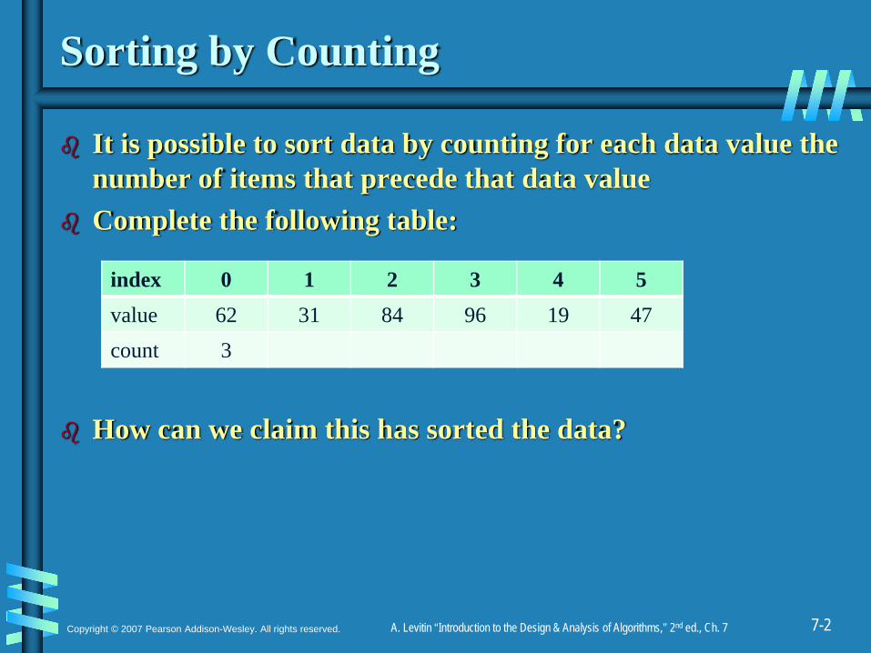
Sorting by Counting

It is possible to sort data by counting for each data value the number of items that precede that data value Complete the following table:

How can we claim this has sorted the data?

index 0 1 2 3 4 5value 62 31 84 96 19 47count 3


Comparison Counting Sort

The algorithm

Complexity Analysis


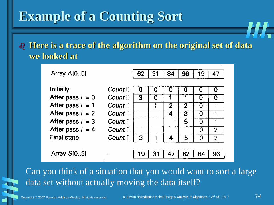
Example of a Counting Sort

Here is a trace of the algorithm on the original set of data we looked at

Can you think of a situation that you would want to sort a large data set without actually moving the data itself?


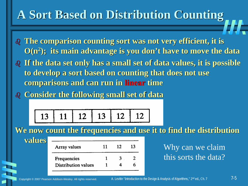
A Sort Based on Distribution Counting

The comparison counting sort was not very efficient, it is O(n2); its main advantage is you don’t have to move the dataIf the data set only has a small set of data values, it is possible to develop a sort based on counting that does not use comparisons and can run in linear timeConsider the following small set of data

We now count the frequencies and use it to find the distribution values

Why can we claim this sorts the data?


The Distribution Counting Algorithm

What is the complexity of this algorithm?


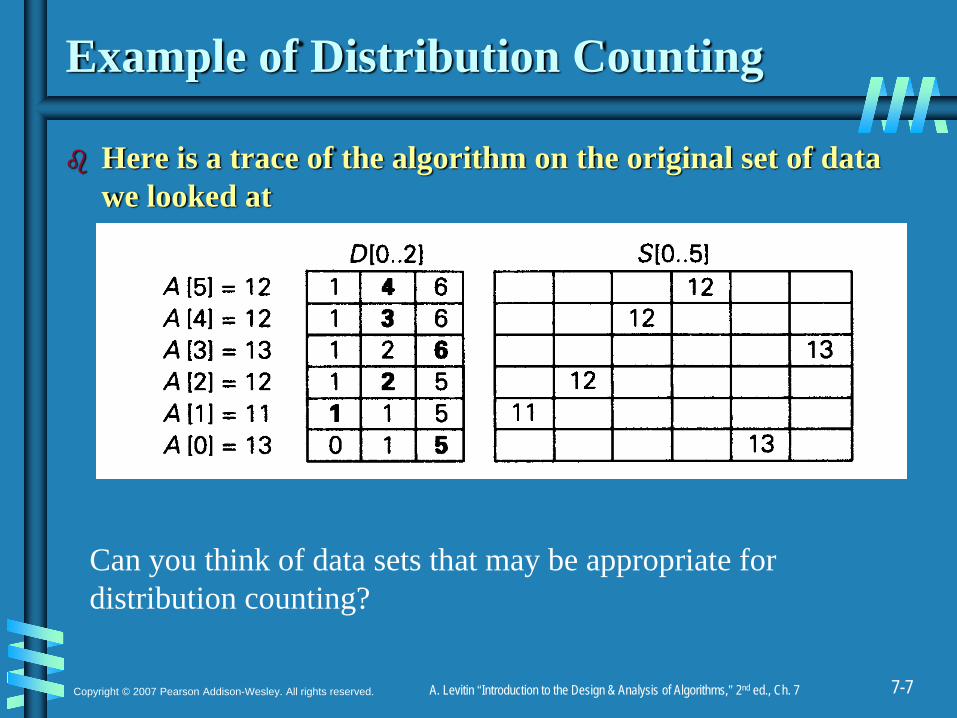
Example of Distribution Counting

Here is a trace of the algorithm on the original set of data we looked at

Can you think of data sets that may be appropriate for distribution counting?


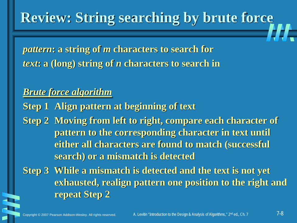
Review: String searching by brute force

pattern: a string of m characters to search fortext: a (long) string of n characters to search in

Brute force algorithmStep 1 Align pattern at beginning of textStep 2 Moving from left to right, compare each character of

pattern to the corresponding character in text until either all characters are found to match (successful search) or a mismatch is detected

Step 3 While a mismatch is detected and the text is not yet exhausted, realign pattern one position to the right and repeat Step 2


String searching by preprocessing

Several string searching algorithms are based on the inputenhancement idea of preprocessing the pattern

Knuth-Morris-Pratt (KMP) algorithm preprocesses pattern left to right to get useful information for later searching

Boyer -Moore algorithm preprocesses pattern right to left and store information into two tables

Horspool’s algorithm simplifies the Boyer-Moore algorithm by using just one table


Horspool’s Algorithm

A simplified version of Boyer-Moore algorithm:

• preprocesses pattern to generate a shift table that determines how much to shift the pattern when a mismatch occurs

• always makes a shift based on the text’s character c aligned with the last character in the pattern according to the shift table’s entry for c


How far to shift?

Look at first (rightmost) character in text that was compared: The character is not in the pattern

.....c...................... (c not in pattern)BAOBAB

The character is in the pattern (but not the rightmost).....O...................... (O occurs once in pattern)BAOBAB.....A...................... (A occurs twice in pattern)BAOBAB

The rightmost characters do match.....B...................... BAOBAB


Shift tableShift sizes can be precomputed by the formula

distance from c’s rightmost occurrence in patternamong its first m-1 characters to its right end

t(c) = pattern’s length m, otherwise

by scanning pattern before search begins and stored in atable called shift table

Shift table is indexed by text and pattern alphabet Eg, for BAOBAB:

A B C D E F G H I J K L M N O P Q R S T U V W X Y Z

1 2 6 6 6 6 6 6 6 6 6 6 6 6 3 6 6 6 6 6 6 6 6 6 6 6


Example of Horspool’s alg. application

BARD LOVED BANANASBAOBAB

BAOBABBAOBAB

BAOBAB (unsuccessful search)


1 2 6 6 6 6 6 6 6 6 6 6 6 6 3 6 6 6 6 6 6 6 6 6 6 6

_

6


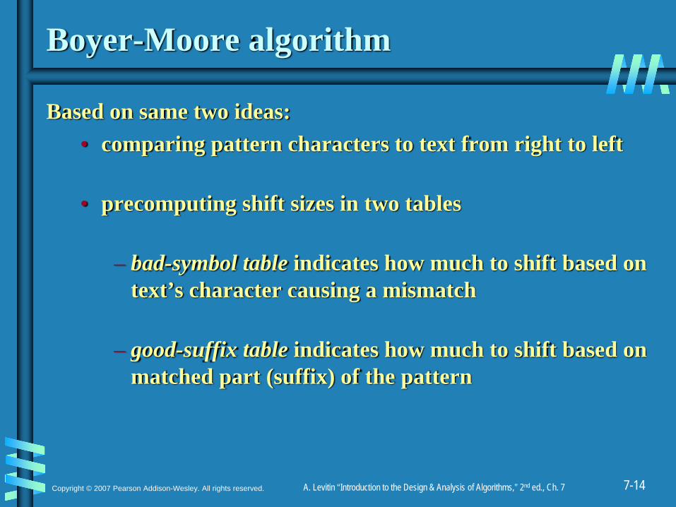
Boyer-Moore algorithm

Based on same two ideas:• comparing pattern characters to text from right to left

• precomputing shift sizes in two tables

– bad-symbol table indicates how much to shift based on text’s character causing a mismatch

– good-suffix table indicates how much to shift based on matched part (suffix) of the pattern


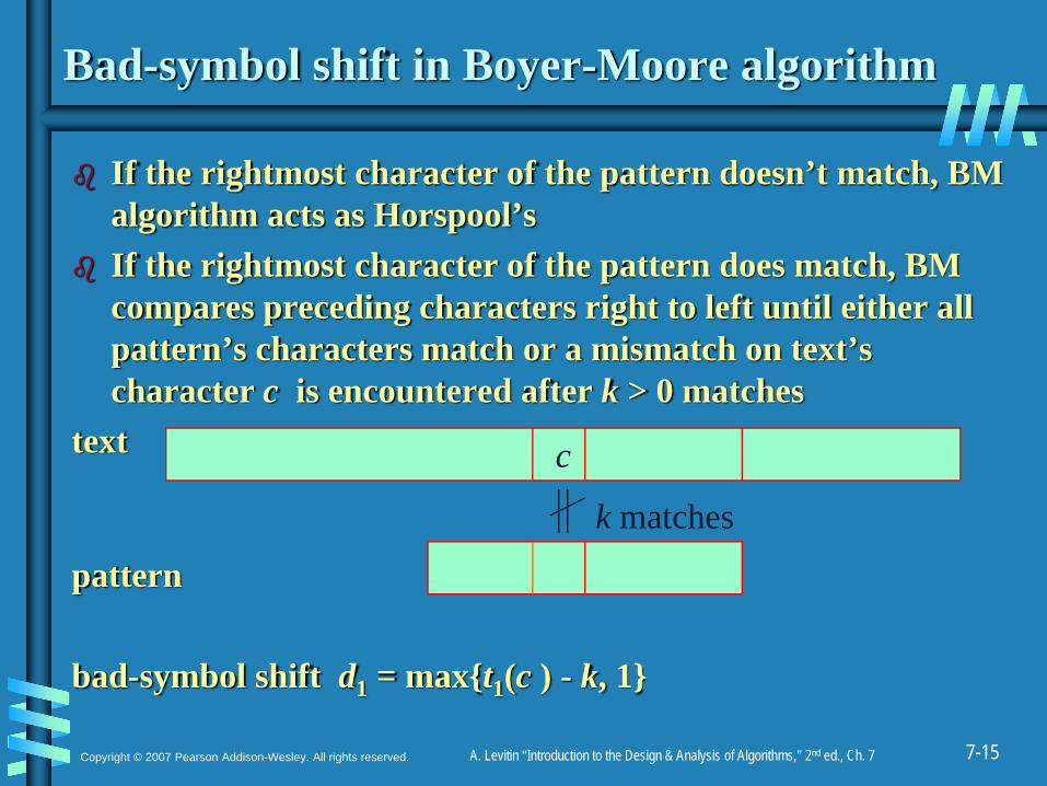
Bad-symbol shift in Boyer-Moore algorithm

If the rightmost character of the pattern doesn’t match, BM algorithm acts as Horspool’sIf the rightmost character of the pattern does match, BM compares preceding characters right to left until either all pattern’s characters match or a mismatch on text’s character c is encountered after k > 0 matches

text

pattern

bad-symbol shift d1 = max{t1(c ) - k, 1}

c

k matches


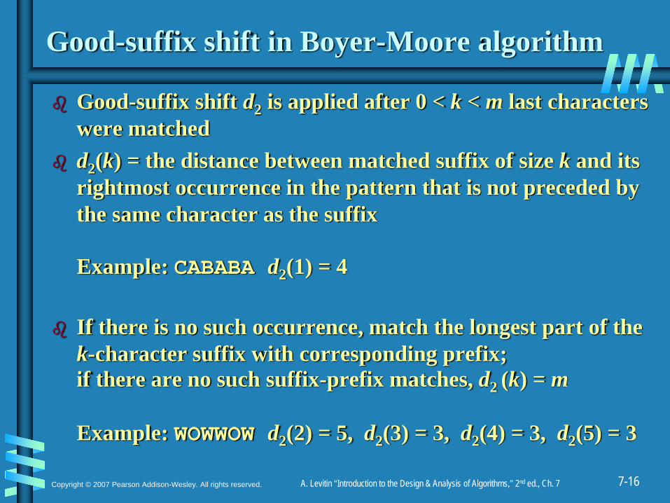
Good-suffix shift in Boyer-Moore algorithm

Good-suffix shift d2 is applied after 0 < k < m last characters were matchedd2(k) = the distance between matched suffix of size k and its rightmost occurrence in the pattern that is not preceded by the same character as the suffix

Example: CABABA d2(1) = 4

If there is no such occurrence, match the longest part of the k-character suffix with corresponding prefix; if there are no such suffix-prefix matches, d2 (k) = m

Example: WOWWOW d2(2) = 5, d2(3) = 3, d2(4) = 3, d2(5) = 3


Boyer-Moore Algorithm

After matching successfully 0 < k < m characters, the algorithm shifts the pattern right by

d = max {d1, d2}where d1 = max{t1(c) - k, 1} is bad-symbol shift

d2(k) is good-suffix shift

Example: Find pattern AT_THAT inWHICH_FINALLY_HALTS. _ _ AT_THAT


Boyer-Moore Algorithm (cont.)

Step 1 Fill in the bad-symbol shift tableStep 2 Fill in the good-suffix shift tableStep 3 Align the pattern against the beginning of the textStep 4 Repeat until a matching substring is found or text ends:

Compare the corresponding characters right to left. If no characters match, retrieve entry t1(c) from the bad-symbol table for the text’s character c causing the mismatch and shift the pattern to the right by t1(c).If 0 < k < m characters are matched, retrieve entry t1(c) from the bad-symbol table for the text’s character c causing the mismatch and entry d2(k) from the good-suffix table and shift the pattern to the right by

d = max {d1, d2}where d1 = max{t1(c) - k, 1}.


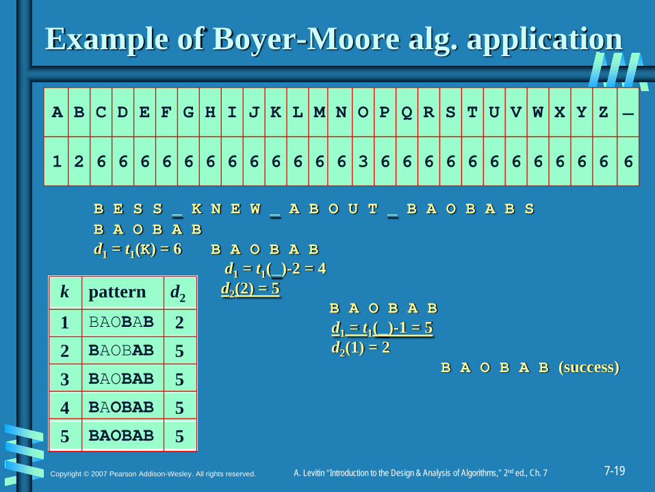
Example of Boyer-Moore alg. application

B E S S _ K N E W _ A B O U T _ B A O B A B SB A O B A Bd1 = t1(K) = 6 B A O B A B

d1 = t1(_)-2 = 4d2(2) = 5

B A O B A Bd1 = t1(_)-1 = 5d2(1) = 2

B A O B A B (success)


1 2 6 6 6 6 6 6 6 6 6 6 6 6 3 6 6 6 6 6 6 6 6 6 6 6

_

6

k pattern d2

1 BAOBAB 22 BAOBAB 53 BAOBAB 54 BAOBAB 55 BAOBAB 5


Hashing

A very efficient method for implementing a dictionary, i.e., a set with the operations:

– find – insert – delete

Based on representation-change and space-for-time tradeoff ideas

Important applications:– symbol tables– databases (extendible hashing)


Hash tables and hash functions

The idea of hashing is to map keys of a given file of size n intoa table of size m, called the hash table, by using a predefinedfunction, called the hash function,

h: K → location (cell) in the hash table

Example: student records, key = SSN. Hash function:h(K) = K mod m where m is some integer (typically, prime)If m = 1000, where is record with SSN= 314159265 stored?

Generally, a hash function should:• be easy to compute• distribute keys about evenly throughout the hash table


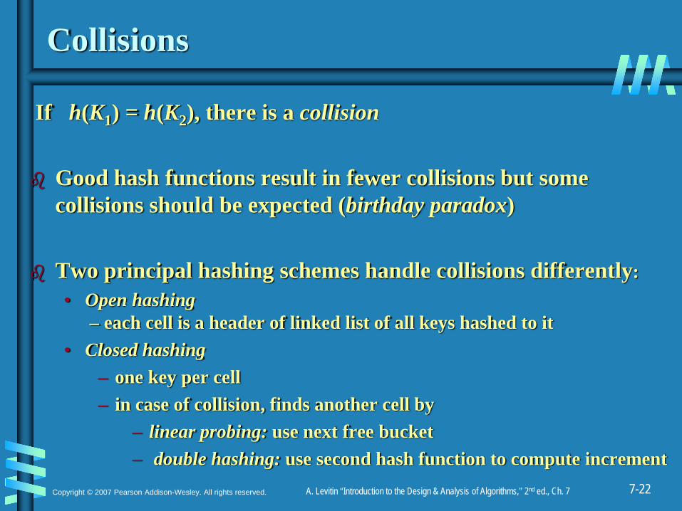
Collisions

If h(K1) = h(K2), there is a collision

Good hash functions result in fewer collisions but some collisions should be expected (birthday paradox)

Two principal hashing schemes handle collisions differently: • Open hashing

– each cell is a header of linked list of all keys hashed to it• Closed hashing

– one key per cell – in case of collision, finds another cell by

– linear probing: use next free bucket – double hashing: use second hash function to compute increment


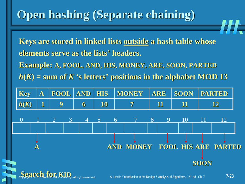
Open hashing (Separate chaining)

Keys are stored in linked lists outside a hash table whoseelements serve as the lists’ headers.Example: A, FOOL, AND, HIS, MONEY, ARE, SOON, PARTED

h(K) = sum of K ‘s letters’ positions in the alphabet MOD 13

Key A FOOL AND HIS MONEY ARE SOON PARTEDh(K) 1 9 6 10 7 11 11 12

A FOOLAND HISMONEY ARE PARTED

SOON

1211109876543210

Search for KID


Open hashing (cont.)

If hash function distributes keys uniformly, average length of linked list will be α = n/m. This ratio is called load factor.

Average number of probes in successful, S, and unsuccessful searches, U:

S ≈ 1+α/2, U = α

Load α is typically kept small (ideally, about 1)

Open hashing still works if n > m


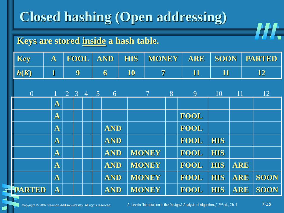
Closed hashing (Open addressing)Keys are stored inside a hash table.

AA FOOLA AND FOOLA AND FOOL HISA AND MONEY FOOL HISA AND MONEY FOOL HIS AREA AND MONEY FOOL HIS ARE SOON

PARTED A AND MONEY FOOL HIS ARE SOON

Key A FOOL AND HIS MONEY ARE SOON PARTED

h(K) 1 9 6 10 7 11 11 12

0 1 2 3 4 5 6 7 8 9 10 11 12


Closed hashing (cont.)Does not work if n > mAvoids pointersDeletions are not straightforwardNumber of probes to find/insert/delete a key depends on load factor α = n/m (hash table density) and collision resolution strategy. For linear probing:

S = (½) (1+ 1/(1- α)) and U = (½) (1+ 1/(1- α)²)As the table gets filled (α approaches 1), number of probes in linear probing increases dramatically:


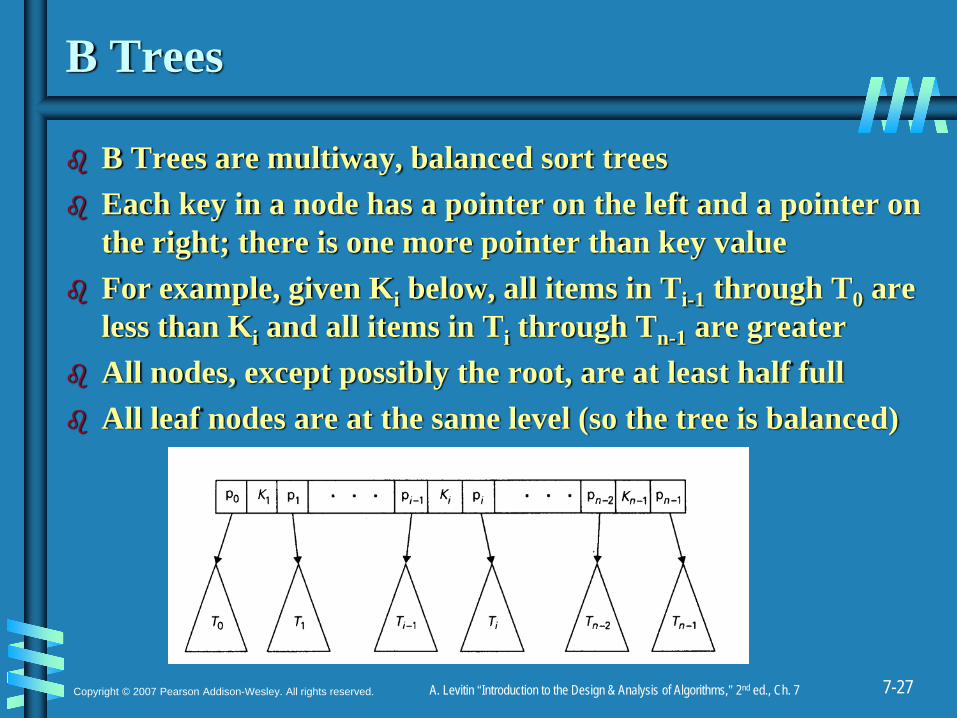
B Trees

B Trees are multiway, balanced sort treesEach key in a node has a pointer on the left and a pointer on the right; there is one more pointer than key valueFor example, given Ki below, all items in Ti-1 through T0 are less than Ki and all items in Ti through Tn-1 are greaterAll nodes, except possibly the root, are at least half fullAll leaf nodes are at the same level (so the tree is balanced)


B-Trees and Disk Drives - 1

Any node contains n[x] keys and n[x]+1 childrenBranching factors are typically between 50 - 2000Height is very shallow minimizing disk accessesThe node size matches the sector size on the disk


Delays in Disk Access

There are three delays associated with reading or writing data to a disk. What are these delay and what are typical values for drives you would purchase for a PC?


B-Trees and Disk Drives - 2

Assume a branching factor of 1000Only the root node is kept in memoryWith one disk access over 1,000,000 keys are accessed; with two disk accesses over one billion keys can be accessed


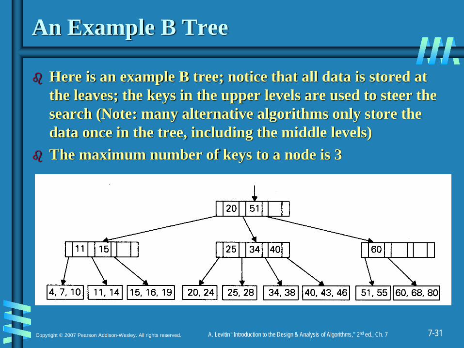
An Example B Tree

Here is an example B tree; notice that all data is stored at the leaves; the keys in the upper levels are used to steer the search (Note: many alternative algorithms only store the data once in the tree, including the middle levels)The maximum number of keys to a node is 3


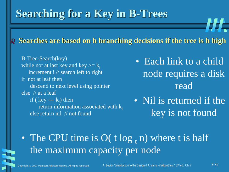
Searching for a Key in B-Trees

Searches are based on h branching decisions if the tree is h high

• Each link to a child node requires a disk

read• Nil is returned if the

key is not found

• The CPU time is O( t log t n) where t is half the maximum capacity per node

B-Tree-Search(key)while not at last key and key >= ki

increment i // search left to rightif not at leaf then

descend to next level using pointerelse // at a leaf

if ( key == ki) then return information associated with ki

else return nil // not found


Inserting in B-Trees

We first search the tree down to the leaf level to see if the key is already present, if we find the key we change the associated data as appropriateIf the key is not found, we insert the key and associated data in the leaf node last visited

If there is room for the new key, we are doneIf there is no room, this causes an overflow; we split the values in the leaf node and pass the middle key back up to the parent nodeThe pointer to the left of this new key value points to the first of the split nodes; the pointer to the right of the new key points to the second of the split nodesIf the parent overflows, its middle value is passed upThis process can continue until the root is reachedIf the root is split a new root node is created with a single key value and the tree has grown in height


Given the tree

Assume the value 65 is inserted

chapter 7: space and time tradeoffs

Documents