chapter 7 techniques of integrationusers.rowan.edu/~hassen/mathematica/mathematica for...chapter 7...
TRANSCRIPT
Chapter 7 Techniques of Integration
ü 7.1 Numerical Integration
Students should read Section 7.1 of Rogawski’s Calculus [1] for a detailed discussion of the material presented in thissection.
Numerical integration is the process of approximating a definite integral using appropriate sums of function values. We already
saw in Chapter 5 of this text formulas for Right, Left, and Midpoint Rules and their subroutines LRSUM, RRSUM, and
MRSUM, respectively. In this section, we will develop two additional rules: the Trapezoidal Rule and Simpson’s Rule.
ü 7.1.1 Trapezoidal Rule
The Trapezoidal Rule approximates the definite integral a
bf x „ x by using areas of trapezoids and is given by the formula:
Tn = .5 b - a n y0 + 2 y1 + ... + 2 yn-1 + ynwhere n is the number of trapezoids and yi = f a + i b - a n . This formula can be found in your calculus text. Here is a
Mathematica subroutine, called TRAP, for implementing the Trapezoidal Rule:
In[1]:= Clearf, a, b, nIn[2]:= TRAPa_, b_, n_ :
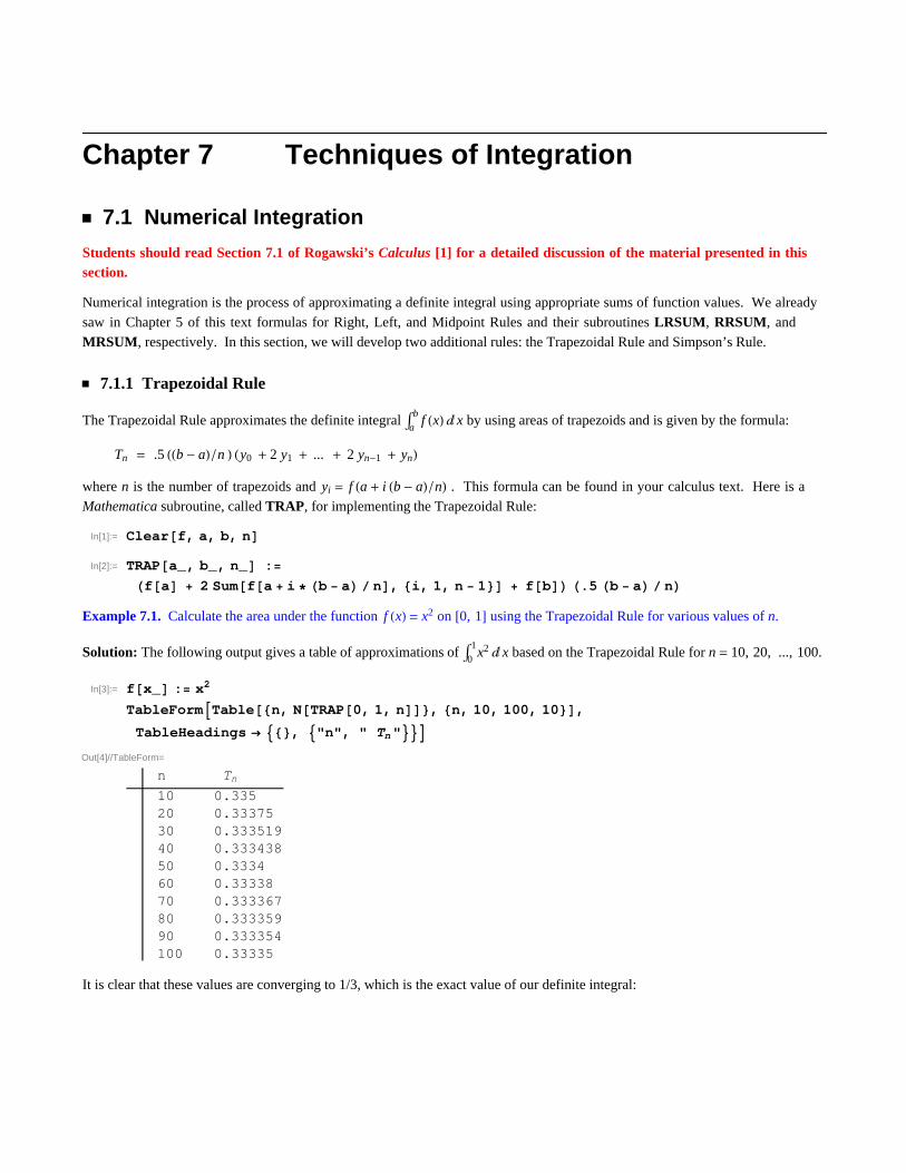
fa 2 Sumfa i b a n, i, 1, n 1 fb .5 b a nExample 7.1. Calculate the area under the function f x = x2 on 0, 1 using the Trapezoidal Rule for various values of n.
Solution: The following output gives a table of approximations of 01x2 „ x based on the Trapezoidal Rule for n = 10, 20, ..., 100.
In[3]:= fx_ : x2
TableFormTablen, NTRAP0, 1, n, n, 10, 100, 10,
TableHeadings , "n", " Tn "Out[4]//TableForm=
n Tn
10 0.33520 0.3337530 0.33351940 0.33343850 0.333460 0.3333870 0.33336780 0.33335990 0.333354100 0.33335
It is clear that these values are converging to 1/3, which is the exact value of our definite integral:

In[5]:= 0
1
x2 x
Out[5]=1
3
ü 7.1.2 Simpson’s Rule
One difference between Simpson’s Rule and all the other rules we have developed so far (TRAP, LRSUM, RRSUM, and
MRSUM) is that the number of partition points, n, in this case, must be even. The other difference is that Simpson’s Rule is aquadratic approximation based on parabolas, whereas the other rules are linear approximations based on lines. The formula forSimpson’s Rule is given by (refer to your calculus text for details):
Sn = 1 3 y0 + 4 y1 + 2 y2 + 4 y3 + 2 y4 + ... + 4 yn-3 + 2 yn-2 + 4 yn-1 + yn b - a n = 1 3y0 + 4 y1 + y2 + y2 + 4 y3 + y4 + ... + yn-2 + 4 yn-1 + yn b - a n
where yi = f a + i b - a n. Here is a Mathematica subroutine, called SIMP, for implementing Simpson’s Rule:
In[6]:= Cleara, b, nIn[7]:= SIMPa_, b_, n_ :
1 3 Sumfa 2 i 2 b a n 4 fa 2 i 1 b a n
fa 2 i b a n, i, 1, n 2 b a n
Example 7.2. Calculate the area under the function f x = x2 on 0, 1 using Simpson’s Rule for various values of n.
Solution: We use the same set of values of n as in the previous example. This will allow us to compare Simpson’s Rule with theTrapezoidal Rule.
In[8]:= fx_ : x2
TableFormTablen, NSIMP0, 1, n, n, 10, 100, 10,
TableHeadings , "n", " sn "Out[9]//TableForm=
n sn
10 0.33333320 0.33333330 0.33333340 0.33333350 0.33333360 0.33333370 0.33333380 0.33333390 0.333333100 0.333333
Notice how fast SIMP converges to the actual value of the integral (1/3) compared to TRAP.
Example 7.3. Calculate the definite integral of f x = sin25 x2 on 0, 1 using Simpson’s Rule and approximate it to five
decimal places. What is the minimum number of partition points needed to obtain this level of accuracy?
Solution: We first evaluate SIMP using values for n in increments of 20.
2 Mathematica for Rogawski's Calculus
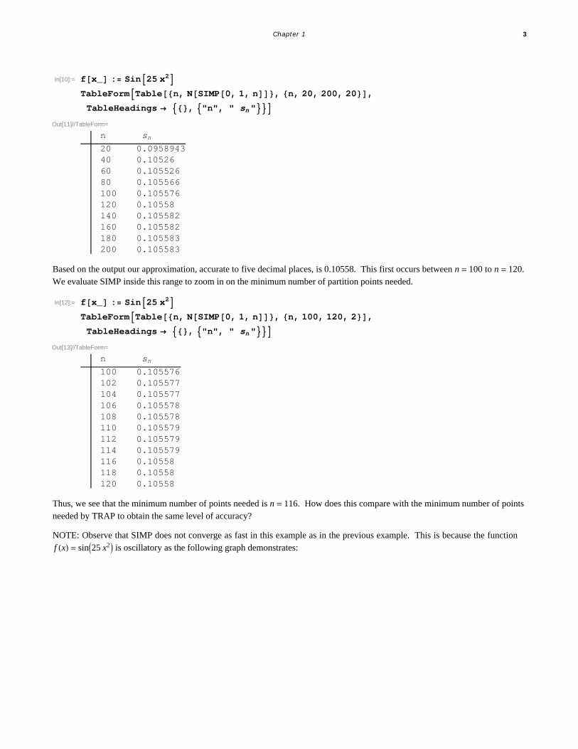
In[10]:= fx_ : Sin25 x2TableFormTablen, NSIMP0, 1, n, n, 20, 200, 20,
TableHeadings , "n", " sn "Out[11]//TableForm=
n sn
20 0.095894340 0.1052660 0.10552680 0.105566100 0.105576120 0.10558140 0.105582160 0.105582180 0.105583200 0.105583
Based on the output our approximation, accurate to five decimal places, is 0.10558. This first occurs between n = 100 to n = 120.We evaluate SIMP inside this range to zoom in on the minimum number of partition points needed.
In[12]:= fx_ : Sin25 x2TableFormTablen, NSIMP0, 1, n, n, 100, 120, 2,
TableHeadings , "n", " sn "Out[13]//TableForm=
n sn
100 0.105576102 0.105577104 0.105577106 0.105578108 0.105578110 0.105579112 0.105579114 0.105579116 0.10558118 0.10558120 0.10558
Thus, we see that the minimum number of points needed is n = 116. How does this compare with the minimum number of pointsneeded by TRAP to obtain the same level of accuracy?
NOTE: Observe that SIMP does not converge as fast in this example as in the previous example. This is because the functionf x = sin25 x2 is oscillatory as the following graph demonstrates:
Chapter 1 3

In[14]:= Plotfx, x, 0, 1
Out[14]=0.2 0.4 0.6 0.8 1.0
-1.0
-0.5
0.5
1.0
Try increasing the frequency of this function, say to sin100 x2, to see how well SIMP performs.
ü 7.1.3 Midpoint Rule
Since most calculus texts include again the Midpoint Rule in the section on numerical integration, for completeness, we will too.The Riemann sum using the midpoints of each subinterval is given by the following formula:
In[15]:= ClearfMRSUMa_, b_, n_ : Sumfa i 1 2 b a n b a n, i, 1, n
Example 7.4. Calculate the area under the function f x = x2 on 0, 1 using the Midpoint Rule for various values of n.
Solution:
In[17]:= fx_ : x2
TableFormTablen, NMRSUM0, 1, n, n, 10, 100, 10,
TableHeadings , "n", "Midpoint rule"Out[18]//TableForm=
n Midpoint rule
10 0.332520 0.33312530 0.33324140 0.33328150 0.333360 0.3333170 0.33331680 0.3333290 0.333323100 0.333325
ü Exercises
1. Consider the definite integral 1
2lnx „ x.
a) Using the Trapezoidal Rule, Simpson's Rule, and Midpoint Rule, approximate this integral for n = 10, 20, ..., 100.
b) Compare how fast each subroutine (TRAP, SIMP, MRSUM) converges to ablnx „ x and decide which of these rules is
"best."
4 Mathematica for Rogawski's Calculus

2. Repeat Exercise 1 for the following definite integrals:
a) 02 ex
x+1„ x b) 0
1cosx2 „ x c) 0
1ex2
„ x
Can you make any general conclusions about which rule (Trapezoidal, Simpson’s, Midpoint) is best?
3. For each of the functions given below, set up a definite integral for the volume of the solid of revolution obtained by revolving
the region under f x along the given interval and about the given axis. Then use the subroutines TRAP, SIMP, and MRSUMto approximate the volume of each solid accurate to two decimal places (use various values of n to obtain the desired accuracy).
a) f x = cos x; 0, p 2; x-axis b) f x = e-x2; 0, 1; y-axis c) f x = sin x, 0, p, x - axis
ü 7.2 Techniques of Integration
Students should read Sections 7.2 trhough 7.4 and 7.6 of Rogawski's Calculus [1] for a detailed discussion of the materialpresented in this section.
All calculus texts have at least a chapter devoted to "Techniques of Integration." When using Mathematica, these techniques areusually not necessary since Mathematica automatically gives you the answer.
ü 7.2.1 Substitution
On occasion, we do need to use techniques of integration, even when using Mathematica.
Example 7.5. Evaluate the following integral: 2x 2x2 - 1 „ x.
Solution: We evaluate this integral in Mathematica:
In[19]:= 2x 2x2 1 x
Out[19]=
2x 1 4x Log2x 1 4x Log4
To students in a first-year calculus course, this answer makes no sense. There are many integrals that Mathematica cannotevaluate at all, or cannot evaluate in terms of elementary functions (such as the integral above). Some of these integrals aredoable in terms we should understand, once we first use an appropriate technique of integration. In the above example, all weneed to do is first make the following substitution: u = 2x and d u = ln 2 2x d x, which transforms the integral to:
In[20]:=1
Log2 u2 1 u
Out[20]=
12
u 1 u2 12
Logu 1 u2 Log2
This is the correct answer. All we need to do is substitute 2x for u, and add the arbitrary constant of integration, getting:
1
2 Log2 ( 2x -1 + 2x2 - Log[2x + -1 + 2x2 ] ) + C
Note that the Mathematica function Log[x] is equivalent to the standard form ln x.
ü 7.2.2 Trigonometric Substitution
Chapter 1 5

Example 7.6. Evaluate 1
x2 x2-9
„ x.
Solution: By hand, the integral 1
x2 x2-9
„ x would normally be evaluated with a trigonometric substitution of the form
x = 3 secq. But with Mathematica, we can do this directly:
In[21]:= 1
x2 x2 - 9
‚ x
Out[21]=9 x2
9 x
This, of course, is the correct answer, when we remember that Mathematica does not add an arbitrary constant to indefiniteintegrals.
ü 7.2.3 Method of Partial Fractions
Integrals of rational expressions often require the Method of Partial Fraction Decomposition to evaluate them (by hand). Forexample:
3 x-3
x2+5 x+4„ x = 5
x+4- 2
x+1 „ x = 5 ln x + 4 -2 ln x + 1 = ln
x+45
x+12
On the other hand, Mathematica will give us essentially the same answer for this integral, but does its work behind the sceneswithout revealing its technique:
In[22]:= Simplify3 x 3
x2 5 x 4x
Out[22]= 2 Log1 x 5 Log4 x
If we would like to see the partial fraction decomposition of the integrand, 3 x-3
x2+5 x+4, Mathematica will also do that for us without
strain by using the Apart command:
In[23]:= Apart 3 x 3
x2 5 x 4
Out[23]= 2
1 x
5
4 x
Example 7.7. Evaluate 2 x3+x2-2 x+2
x2+12 „ x.
Solution: We simply evaluate this integral using Mathematica:
In[24]:= 2 x3 x2 2 x 2
x2 12x
Out[24]=4 x
2 1 x2
3 ArcTanx2
Log1 x2
6 Mathematica for Rogawski's Calculus

But again, if we would like to see the partial fraction decomposition of the integrand, 2 x3+x2-2 x+2
x2+12, then this is straightforward
with Mathematica:
In[25]:= Apart 2 x3 x2 2 x 2
x2 12
Out[25]=1 4 x
1 x22
1 2 x
1 x2
ü Exercises
1. Evaluate 1 + lnx 1 + x ln x2 „ x with Mathematica. If it doesn't give an understandable answer, use a technique of
integration that changes the integral into one that Mathematica will evaluate.
In Exercises 2 through 5, use Mathematica to find the partial fraction decomposition of the given functions and then integratethem:
2. x2+3 x - 44
x-3 x+5 3 x-2 3. 3 x2-4 x+5
x-1 x2+1 4. 25
x x2+2 x+5 5. 10
xx2+2 x+52
In Exercises 6 through 10, use Mathematica to evaluate the given integrals.
6. x2
x2- 432 „ x 7. x3 9 - x2 „ x 8. 1
25+x2
„ x
9. sin5 x „ x 9. tan-1 t
1+t2„ t 10. sinh3 x cosh x „ x
ü 7.3 Improper Integrals
Students should read Section 7.7 of Rogawski's Calculus [1] for a detailed discussion of the material presented in thissection.
Recall that there are two types of improper integrals.
Type I: If we assume that f x is integrable over a, b for all b ¥ a, then the improper integral of f x over a, ¶ is defined as
a
¶f x „ x = limtض a
tf x „ x,
provided this limit exists. Similarly, we define
-¶b f x „ x = limtØ-¶ t
bf x „ x,
provided this limit exists.
Type II: If f x is continuous on a, b but discontinuous at x = b, we define
ab
f x „ x = limtØ b- atf x „ x ,
provided this limit exists. Similarly, if f x is continuous on a, b but discontinuous at x = a,
ab
f x „ x = limtØ a+ tb
f x „ x,
provided this limit exists. Finally, if f x is continuous for all x on a, b except at x = c, where a < c < b, we define
a
bf x „ x = limtØc- a
tf x „ x + limtØc+ t
bf x „ x,
provided both of these limits exist.
Chapter 1 7

By using the Limit command in Mathematica along with Integrate, Mathematica eliminates the drudgery of having to evaluatethese integrals by hand.
Example 7.8. Evaluate the following improper integrals:
a) 20
¶ 1
y„ y
b) 2
¶‰-2 x „ x
c) 01x ln x „ x
d) -¶¶ 1
1+x2„ x
Solution:
a) We evaluate
In[26]:= 20
1
yy
Integrate::idiv : Integral of 1
y does not converge on 20,¶. à
Out[26]= 20
1
yy
Thus, evaluating this integral directly using Mathematica tells us it does not exist. Alternatively, we could have used the limitdefinition:
In[27]:= Limit20
t 1
yy, t
Out[27]=
Observe the difference in the two outputs above. Both correctly express the answer as divergent; however, the second answer isbetter since it reveals the nature of the divergence (infinity), which is the answer we would expect if solving this problem by hand.
b) We evaluate
In[28]:= 2
2 x x
Out[28]=1
2 4
Again, we obtain the same answer using the limit definition (as it should):
In[29]:= Limit2
t
2 x x , t
Out[29]=1
2 4
Mathematica will similarly handle discontinuities. In the following example, the function has a discontinuity at x = 0.
c) We evaluate
8 Mathematica for Rogawski's Calculus

In[30]:= 0
1
x Logx x
Out[30]= 1
4
In[31]:= Limitt
1
x Logx x, t 0, Direction 1
Out[31]= ConditionalExpression 1
4, t Reals 0 Ret 1 Ret 1 &&
t
1 t Reals Re t
1 t 0 Re t
1 t 1
d) We evaluate
In[32]:= -•
• 1
1 + x2‚ x
Out[32]=
Note that Mathematica does not require us to break the integral up into two integrals, which would be required according to itsdefinition, if evaluated by hand. On the other hand, there is nothing wrong with dividing this integral into two in Mathematica:
In[33]:=
0 1
1 x2x
0
1
1 x2x
Out[33]=
NOTE: Observe that it does not matter where we divide the integral. It is valid to express -¶a 1
1+x2„ x + a
¶ 1
1+x2„ x for the
integral -¶¶ 1
1+x2„ x for any real value a as long as they are convergent. However, evaluating this sum in Mathematica yields
different expressions for the answer, which depend on the sign of a and whether it is real or complex. This is shown in thefollowing output:
In[34]:= Cleara
a 1
1 x2x
a
1
1 x2x
Out[35]= ConditionalExpression1
2 Log1 a ¶ ConjugateLog1 a Rea 0 && Ima 0
Log1 a True
1
2 Log1 a ¶ ConjugateLog1 a Rea 0 && Ima 0
Log1 a True, 1
Ima 1
If instead, a is given a fixed value, then Mathematica will give us our answer of p:
Chapter 1 9
In[36]:= a 1
a 1
1 x2x
a
1
1 x2x
Out[36]= 1
Out[37]=
ü Exercises
In Excercises 1 through 8, evaluate the given improper integrals:
1. -¶4 ‰.01 t „ t 2. -3¶ 1
x+432 „ x 3. -24 1
x+213 „ x 4. -¶¶ x ‰-x2„ x
5. 03 1
x-1„ x 6. -¶¶ 1
ex+e-x „ x 7. 1¶ 1
x.999„ x 8. 1
¶ 1
x1.003„ x
11. Find the volume of the solid obtained by rotating the region below the graph of y = ‰-x about the x-axis for 0 § x <¶.
12. Determine how large the number b has to be in order that b¶ 1
x2+1„ x < .0001.
13. Evaluate the improper integral -11 1
x3
„ x.
14. Determine how large the number b should be so that b¶ 1
x2+1„ x < .0001.
15. Consider the function defined by
Gx = 0¶
tx-1 e-t „ t
a) Evaluate Gn for n = 0, 2, , 3, 4, ...., 10. Make a conjecture about these values. Verify your conjecture.b) Evaluate G2 n - 1 2, for n = 1, 2, 3, ... 10. Make a conjecture about these values. Verify your conjecture.c) Plot the graph of Gx on the interval 0, 5.NOTE: The function G is called the gamma function and is denoted by Gx. In Mathematica it is denoted by Gamma[x]. Thegamma function was first introduced by Euler as a generalization of the factorial function.
ü 7.4 Hyperbolic and Inverse Hyperbolic Functions
Students should read Section 7.5 of Rogawski's Calculus [1] for a detailed discussion of the material presented in thissection.
ü 7.4.1. Hyperbolic Functions
The hyperbolic functions are defined in terms of the exponential functions. They have a direct connection to engineeringmathematics, including bridge construction. For example, cables from suspension bridges typically form a curve called acatenary (derived from the Latin word catena, which means chain) that is described by these functions.
The six hyperbolic functions are denoted and defined as follows:
sinh x = ex- e-x
2, cosh x = ex+ e-x
2, tanh x = ex- e-x
ex+ e-x
coth x = ex+ e-x
ex- e-x , sech x = 2
ex+ e-x , csch x = 2
ex- e-x
10 Mathematica for Rogawski's Calculus

The reason these functions are called hyperbolic functions is due to their connection with the equilateral hyperbola x2 - y2 = 1.
Here, one defines x = cosh t and y = sinh t. Hence, one obtains the basic hyperbolic identity cosh2 t - sinh2 t = 1, much the same
manner as the corresponding trigonometric identity cos2 t + sin2 t = 1, when one considers the unit circle x2 + y2 = 1 withx = cos t and y = sin t.
In Mathematica, we use the same notation with the obvious convention that the first letter of each function is capitalized and
square brackets must be used in place of parentheses. Thus, sinh x will be entered as Sinh[x].
Example 7.9. Consider the hyperbolic sine function f x = sinh x.a) Plot the graph of f . b) From the graphs deduce the domain and range of the function. c) Is f bounded? d) Does f attain an absolute minimum? Maximum?e) Repeat a) through d) for the hyperbolic function gx = cosh x f) Repeat a) through d) for the hyperbolic function hx = tanh x.
Solution: We begin by defining f in Mathematica:
In[38]:= Clearf, xfx_ Sinhx
Out[39]= Sinhxa) We next plot its graph on the interval -3, 3.In[40]:= Plotfx, x, 3, 3
Out[40]=-3 -2 -1 1 2 3
-10
-5
5
10
b) The preceding graph indicates that the domain and range of sinh x is -¶, ¶. To convince yourself, you should plot the graphover wider intervals. We should also expect this from the definition of sinh x itself. Can you explain why?
c) The function sinh x is not bounded. The graph earlier should not be used as a proof of this. However, we can evaluate its limitat -¶ and ¶ to see that this is indeed true.
In[41]:= Limitfx, x Limitfx, x
Out[41]=
Out[42]=
d) The limits just computed show that sinh x has no absolute maximum or minimum since it is unbounded.
e) Next, we consider the hyperbolic cosine function denoted by cosh x.
Chapter 1 11

In[43]:= Clearg, xgx_ Coshx
Out[44]= CoshxIn[45]:= Plotgx, x, 3, 3
Out[45]=
-3 -2 -1 1 2 3
4
6
8
10
The preceding graph indicates that the domain of cosh x is -¶, ¶. The range appears to be 1, ¶. Can you prove this?
The hyperbolic cosine function, cosh x, is not bounded from above. This can be seen from the following limits:
In[46]:= LimitCoshx, x LimitCoshx, x
Out[46]=
Out[47]=
Again, since cosh x is not bounded from above, it follows that cosh x has no absolute maximum. As we have observed in part b)of this example, cosh x has absolute minimum value 1, attained at x = 0.
f) Finally, we consider the hyperbolic tangent function, tanh x:
In[48]:= Clearh, xhx_ Tanhx
Out[49]= TanhxIn[50]:= Plothx, x, 3, 3
Out[50]=-3 -2 -1 1 2 3
-1.0
-0.5
0.5
1.0
12 Mathematica for Rogawski's Calculus

Again, the preceding graph indicates that the domain of tanh x is -¶, ¶. The range appears to be -1, 1. This can be seenfrom the following limits:
In[51]:= LimitTanhx, x LimitTanhx, x
Out[51]= 1
Out[52]= 1
The graph of tanh x also indicates that it is strictly increasing on its domain. This can be proven by showing that its derivative,which we will calculate later, is strictly positive. It is clear that tanh x has no absolute extrema.
NOTE: The reader will notice some similarities between the hyperbolic functions and the associated trigonometric functions.Moreover, if one studies the theory of functions of a complex variable, the relationship between these classes of transcendentalfunctions becomes even more transparent; for numerous identities exist between the classes of functions.
ü 7.4.2 Identities Involving Hyperbolic Functions
It is immediate that the ratio and reciprocal identities for the hyperbolic functions coincide with their trigonometric counterparts.In fact, for each trigonometric identity, there is a corresponding (not necessarily the same) hyperbolic identity. Following aresome examples.
Example 7.10. Show that the following identities hold true.
a) 1 - tanh2 x = sech2 x b) coshx + y = cosh x cosh y + sinh x sinh y
Solution:
a) We use the definitions for tanh x and sech x to express each side of the identity in terms of exponentials:
In[53]:= Simplify1 Tanhx2 . Tanhx E^x E^x E^x E^x
Out[53]=4 2 x
1 2 x2
In[54]:= SimplifySechx2 . Sechx 2 E^x E^x
Out[54]=4
x x2
We leave it for the reader to verify that both of these outputs agree, that is, 4 e2 x
1+e2 x2 =4
e-x+ex2 (cross-multiply and then simplify).
The identity can also be confirmed in Mathematica by evaluating the difference between its left- and right-hand sides, whichshould equal zero:
In[55]:= Simplify1 Tanhx2 Sechx2Out[55]= 0
NOTE: We can also confirm the identity graphically by plotting the graphs of each side of the identity, which should coincide.
Chapter 1 13

In[56]:= Plot1 Tanhx^2, Sechx^2, x, 2, 2
Out[56]=
-2 -1 1 2
0.2
0.4
0.6
0.8
1.0
b) We again evaluate the difference between the left- and right-hand sides of the identity:
In[57]:= SimplifyCoshx y Coshx Coshy Sinhx SinhyOut[57]= 0
ü 7.4.3 Derivatives of Hyperbolic Functions
We next contrast the formulas for the derivatives of the trigonometric functions versus the formulas for the derivatives of thecompanion hyperbolic functions.
Example 7.11. Compare the derivatives of the given pair of functions.a) sinh x and sin x b) cosh x and cos x c) tanh x and tan x
Solution: We use the derivative command, D, to evaluate derivatives of each pair.
a)
In[58]:= DSinhx, xDSinx, x
Out[58]= CoshxOut[59]= Cosxb)
In[60]:= DCoshx, xDCosx, x
Out[60]= SinhxOut[61]= Sinxb)
In[62]:= DTanhx, xDTanx, x
Out[62]= Sechx2
Out[63]= Secx2
14 Mathematica for Rogawski's Calculus

It is clear that derivatives of hyperbolic and trigonometric functions are quite similar.
ü 7.4.4 Inverse Hyperbolic Functions
In light of the fact that hyperbolic functions are defined in terms of the exponential functions, it is readily apparent that theinverse hyperbolic functions are defined in terms of the natural logarithmic function. The inverses of the hyperbolic functions
have notation similar to those of inverse trigonometric functions. Thus, the inverse of sinh x is denoted by arcsinh x or sinh-1 x.
In Mathematica, the notation is sinh-1 x is ArcSinh[x].
Example 7.12. Plot the graphs of sinh-1 x and sinh x on the same axis.
Solution: Recall that the graph of a function and the graph of its inverse are reflections of each other across the line y = x. This
is confirmed by the following plot of sinh-1 x (in blue) and sin x (in red).
In[64]:= PlotSinhx, x, ArcSinhx, x, 3, 3,PlotStyle Blue, Green, Red, AspectRatio Automatic, PlotRange 3, 3
Out[64]=-3 -2 -1 1 2 3
-3
-2
-1
1
2
3
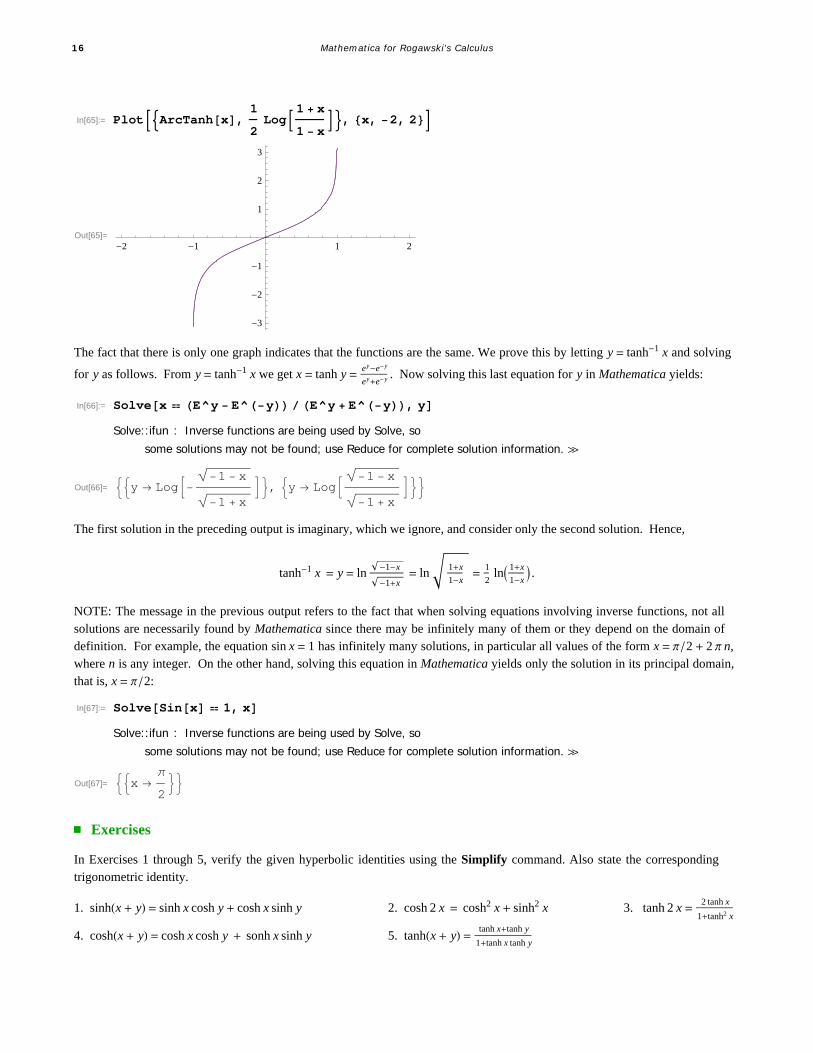
Example 7.13. Show that tanh-1 x = 1
2ln 1+x
1-x for -1 < x < 1.
Solution: We plot the graphs of y = tanh-1 x and y = 1
2ln 1+x
1-x on the same axes. Note that Mathematica's notation of tanh-1 x is
ArcTanh [x] and ln y is entered as Log[y]:
Chapter 1 15
In[65]:= PlotArcTanhx,1
2Log 1 x
1 x, x, 2, 2
Out[65]=-2 -1 1 2
-3
-2
-1
1
2
3
The fact that there is only one graph indicates that the functions are the same. We prove this by letting y = tanh-1 x and solving
for y as follows. From y = tanh-1 x we get x = tanh y = ey-e-y
ey+e-y . Now solving this last equation for y in Mathematica yields:
In[66]:= Solvex E^y E^y E^y E^y, ySolve::ifun : Inverse functions are being used by Solve, so
some solutions may not be found; use Reduce for complete solution information. à
Out[66]= y Log 1 x
1 x, y Log 1 x
1 x
The first solution in the preceding output is imaginary, which we ignore, and consider only the second solution. Hence,
tanh-1 x = y = ln -1-x
-1+x= ln 1+x
1-x= 1
2ln 1+x
1-x .
NOTE: The message in the previous output refers to the fact that when solving equations involving inverse functions, not allsolutions are necessarily found by Mathematica since there may be infinitely many of them or they depend on the domain ofdefinition. For example, the equation sin x = 1 has infinitely many solutions, in particular all values of the form x = p 2 + 2 p n,where n is any integer. On the other hand, solving this equation in Mathematica yields only the solution in its principal domain,that is, x = p 2:
In[67]:= SolveSinx 1, xSolve::ifun : Inverse functions are being used by Solve, so
some solutions may not be found; use Reduce for complete solution information. à
Out[67]= x
2
ü Exercises
In Exercises 1 through 5, verify the given hyperbolic identities using the Simplify command. Also state the correspondingtrigonometric identity.
1. sinhx + y = sinh x cosh y + cosh x sinh y 2. cosh 2 x = cosh2 x + sinh2 x 3. tanh 2 x = 2 tanh x
1+tanh2 x
4. coshx + y = cosh x cosh y + sonh x sinh y 5. tanhx + y = tanh x+tanh y
1+tanh x tanh y
16 Mathematica for Rogawski's Calculus

6. Determine the first few positive integral powers of cosh x + sinh x. Can you form a general conjecture for the nth case,namely cosh x + sinh xn, where n is any natural number? Then justify your conclusion via mathematical induction.
In Exercises 7 through 12, determine the derivatives of thegiven functions and simplify your answers where possible. Compareyour solution via paper and pencil methods with the one generated by Mathematica.
7. f x = tanh 1 + x2 8. f x = x sinh x - cosh x 9. f x = 1+tanh x
1- tanh x
10. f x = x2 sinh-12 x 11. f x = x tanh-1 x + ln 1 - x2 12. f x = x coth x - sech x
13. The Gateway Arch in St. Louis was designed by Eero Saarinen and was constructed using the equation
y = 211.49 - 20.96 cosh 0.03291765 x for the central curve of the arch, where x and y are measured in meters and x § 91.20.
a) Plot the graph of the central curve.b) What is the height of the arch at its center?c) At what points is the arch 100 meters in height?d) What is the slope of the arch at the points in part (c)?
14. A flexible cable always hangs in the shape of a catenary y = c + a cosh x a, where c and a are constants and a > 0. Plotseveral members of the family of functions y = a cosh x a for various values of a. How does the graph change as a varies?
In Exercises 15 through 17, evaluate each of the given integrals:
15. sinh x coshn x „ x 16. cosh x
cosh2 x-1„ x 17. sech2 x
2+tanh x„ x
18. Let t = ln 1+ 5
2 and define
f n = 2
5cosht n, if n is odd
2
5sinh t n, if n is even
Evaluate f n for n = 1, 2, 3, ..., 20. Do these values seem familiar? If not, we highly recommend the interesting article byThomas Osler, Vieta-like products of nested radicals with Fibonacci and Lucas numbers, to appear in the journal FibonacciQuarterly.
Chapter 1 17

Chapter 8 Further Applications of Integration
ü 8.1 Arc Length and Surface Area
Students should read Section 8.1 of Rogawski's Calculus [1] for a detailed discussion of the material presented in thissection.
ü 8.1.1 Arc Length
The integrals for calculating arc length and surface area are generally difficult to do by hand. Thus, Mathematica is the appropri-ate tool for evaluating these integrals.
If y is a function of x, that is, y = f x, and f ' x exists and is continuous on a, b, then the arc length of the graph of f x overthe interval a, b is
L = a
b1 + f ' x2 „ x
If x is a function of y, that is, x = g y, and g ' y exists and is continuous on c, d, then the arc length of the graph of g y overthe interval c, d is
L = cd
f ' y2 + 1 „ y
Example 8.1. Estimate the arc length of y = 1
x over the interval 1, 2.
Solution: Finding the arc length of this simple rational function by hand is virtually impossible. This is because f ' x = - 1
x2 and
thus the arc length integral is L = 12
1 + 1
x4„ x, which cannot be evaluated in terms of elementary functions, as the following
answer illustrates.
In[68]:= 1
2
1 1
x4x
Out[68]=
2 Gamma 74
3 Gamma 54
1
2Hypergeometric2F1 1
2,
1
4,
3
4, 16
However, there are numerical techniques that we can use. For example, the Mathematica command NIntegrate uses sophisti-cated algorithms to gives us a good estimate for this definite integral:
In[69]:= NIntegrate 1 1
x4, x, 1, 2
Out[69]= 1.13209
A more elementary method of estimating this arc length is Simpson's Rule as shown in Section 7.1 of this text.
18 Mathematica for Rogawski's Calculus

In[70]:= Clearf, a, b, nSIMPa_, b_, n_, f_ :
1 3 Sumfa 2 i 2 b a n 4 fa 2 i 1 b a n
fa 2 i b a n, i, 1, n 2 b a n
In[72]:= fx_ : 1 1
x4
TableFormTablen, NSIMP1, 2, n, f, n, 10, 100, 10,
TableHeadings , "n", "Sn " Out[73]//TableForm=
n Sn
10 1.132120 1.1320930 1.1320940 1.1320950 1.1320960 1.1320970 1.1320980 1.1320990 1.13209100 1.13209
Thus, we see that Simpson's Rule gives us as accurate an estimate of the arc length, as does the NIntegrate command for n assmall as 20.
Example 8.2. Consider the the ellipse whose equation is given by
x2
a2+
y2
b2= 1
Assume that a > b. Find the arc length of the upper half of the ellipse.
Solution: To plot the ellipse for various values of a and b, we define a plotting command plot[a,b] as follows.
In[74]:= Cleara, b, x, y, eq, plot
eqx_, y_, a_, b_ :x2
a2
y2
b2 1
plota_, b_ : ContourPloteqx, y, a, b 0, x, a, a, y, b, b,
AspectRatio Automatic, Axes True, Frame FalseHere is a plot of the ellipse for a = 2 and b = 3.
Chapter 2 19

In[77]:= plot2, 3
Out[77]=-2 -1 1 2
-3
-2
-1
1
2
3
On the upper half of the ellipse, we have y ¥ 0. Thus, we can solve for y and and take the positive solution. We will denote thispositive solution as a function of x, a, and b.
In[78]:= sol Solvex2
a2
y2
b2 1, y;
fx_, a_, b_ sol2, 1, 2
Out[79]=b a2 x2
a
Clearly, the domain of f is -a, a. The natural thing to do would be to evaluate the integral -a
a1 + f ' x2 „ x. Try this
yourself, but be prepared to wait awhile. Moreover, Mathematica will give the following output:
IfIma 0 && a Im 1
a2 b2
1
1 a Im 1
a2 b2
0 a Im 1
a2 b2
0 a Re 1
a2 b2
0 ,1
a b2
2 a32 b2 EllipticE1 b2
a2 Signa, Integrate 1
b2 x2
a4 a2 x2, x, a, a,
Assumptions Reb 0 && Rea 0 && Ima 0 && Imb 0 Ima 0 Ima 0
To understand this output, let us make a change of variable x = a sin t. Then the integral becomes (verify this)
-a
a1 + f ' x2 „ x = a -p2p2
1 + b2 sin2 t
a2 cos2 tcos t d t
20 Mathematica for Rogawski's Calculus

The latter integral can be expressed as
2 a 0p2
1 + b2 sin2 t
a2 cos2 tcos t d t = 2 a 0
p2cos2 t + b2 a2 sin2 t d t = 2 a 0
p21 - c2 sin2 t d t ,
where c = 1 - b a2 and we have used the identity cos2 t = 1 - sin2 t.
To simplify our notation, let us define the integrand in the preceding far left integral as
In[80]:= gt_, a_, b_ 1 1 b a2 Sint2
Out[80]= 1 1 b2
a2Sint2
Here are some values of the arc length of the upper half of the ellipse.
In[81]:= TableFormTable2 a 0
2
gt, a, b t, a, 1, 3, b, 1, 3,
TableHeadings "a1", "a2", "a3", "b1", "b2", "b3" Out[81]//TableForm=
b1 b2 b3a1 2 EllipticE3 2 EllipticE8a2 4 EllipticE 3
4 2 4 EllipticE 5
4
a3 6 EllipticE 89 6 EllipticE 5
9 3
Observe that we obtain exact values for the arc length when a = b. Can you explain why?
The approximate values of the numbers appearing in the preceding table are as follows:
In[82]:= TableFormNTable2 a 0
2
gt, a, b t, a, 1, 3, b, 1, 3, 10,
TableHeadings "a1", "a2", "a3", "b1", "b2", "b3" Out[82]//TableForm=
b1 b2 b3a1 3.141592654 4.844224110 6.682446610a2 4.844224110 6.283185307 7.932719795a3 6.682446610 7.932719795 9.424777961
NOTE: The integral 1 - c2 sin2 t „ t is known as an elliptic integral. It is very useful in mathematics and has many applica-
tions. In Mathematica, it is denoted by Elliptic[t,c^2]. The command Elliptic[x,m] gives 0
x1 -m sin2 t dt, while Elliptic[m]
gives 0
p21 -m sin2 t dt.
ü 8.1.2 Surface Area
If f ' x exists and is continuous on a, b, then the surface area of revolution obtained by rotating the graph of f x about the x-axis for a § x § b is
Chapter 2 21
S = 2 p ab
f x 1 + f ' x2 „ x
Similarly, if x = gy and g ' y exists and is continuous on c, d, then the surface area of revolution obtained by rotating g yabout the y-axis for c § y § d is
S = 2 p c
dgy g ' y2 + 1 „ y
Again, evaluating these complicated integrals is what Mathematica does best, as the following examples illustrate.
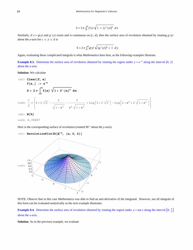
Example 8.3. Determine the surface area of revolution obtained by rotating the region under y = ‰-x along the interval 0, 2about the x-axis.
Solution: We calculate
In[83]:= Clearf, xfx_ : x
S 2 0
2
fx 1 f'x2 x
Out[85]=1
2 4 2 2
2
1 4
2
4 1 4
Log3 2 2 Log2 4 2 1 4
In[86]:= NOut[86]= 6.35887
Here is the corresponding surface of revolution (rotated 90 ° about the y-axis):
In[87]:= RevolutionPlot3DEx, x, 0, 2
Out[87]=
NOTE: Observe that in this case Mathematica was able to find an anti-derivative of the integrand. However, not all integrals ofthis form can be evaluated analytically as the next example illustrates.
Example 8.4. Determine the surface area of revolution obtained by rotating the region under y = tan x along the interval 0, p
4
about the x-axis.
Solution: As in the previous example, we evaluate
22 Mathematica for Rogawski's Calculus

In[88]:= Clearf, xfx_ : TanxNIntegrate2 fx 1 f'x2 , x, 0, Pi 4
Out[90]= 3.83908
To appreciate the complexity of the integral and understand why we used the command NIntegrate, we advise the reader to
define the anti-derivative F[t] below and evaluate F[p/4] (be prepared to wait awhile).
In[91]:= Ft_ : Integratefx 1 f'x2 , x, 0, tHere is the corresponding surface of revolution:
In[92]:= RevolutionPlot3DTanx, x, 0, Pi 4
Out[92]=
ü Exercises
In Exercises 1 and 2, calculate the arc length of the given function over the given interval:
1. y = x4, over 1, 2 2. y = sin x, over 0,p
2
3. Calculate the arc length of the astroid x23 + y23 = 1. Below is a plot of its graph. Hint: By symmetry it suffices to calculateonly the portion in the first quadrant.
Chapter 2 23

In[93]:= ContourPlotx^2^1 3 y^2^1 3 1, x, 1, 1, y, 1, 1
Out[93]=
-1.0 -0.5 0.0 0.5 1.0-1.0
-0.5
0.0
0.5
1.0
4. Show that the circumference of the unit circle is 2p by calculating its arc length. Use the fact that the equation of the unitcircle is given by x2 + y2 = 1.
In Exercises 5 through 7, compute the surface area of the given functions rotated about the x-axis over the given intervals:
5. y = x3 + 1
x, over 1, 4 6. y = 4 - x2323
over 0, 8 7. y = cos x, over 0, p 8. Show that the surface area of the unit sphere is 4p by rotating the top half of the unit circle x2 + y2 = 1 about the x-axis.
ü 8.2 Center of Mass
Students should read Section 8.3 of Rogawski's Calculus [1] for a detailed discussion of the material presented in thissection.
A lamina is a thin plate whose mass is distributed throughout a region in the plane. Suppose a lamina has a constant density r andthat the lamina occupies a region in the plane under the graph of a continuous function f over the interval a, b, where f x ¥ 0for all x.
The mass of the lamina is given by
M = r ab
f x „ x
Then the moments of the lamina with respect to x-axis and y-axis are denoted by Mx and My and are defined by
Mx =1
2r a
b f x2 „ x
My = r abx f x „ x
The center of mass (also called the centroid) of the lamina is defined to be x, y, where
x =My
M and y = Mx
M
NOTE: If the lamina described above as a density r that continuously depends on x, that is, if r = rx for x in the interval a, b,then the moments, the total mass, and the center of mass are given by
M = abrx f x „ x
24 Mathematica for Rogawski's Calculus

Mx =1
2 a
brx f x2 „ x
My = a
bx rx f x „ x
x =My
M and y = Mx
M
Example 8.5. Suppose a lamina lies underneath the graph of y = 16 - x2 and over the interval -4, 4.
a) Assume the density of the lamina is r = 3. Find the mass, moments, and the center of mass of the lamina. b) Assume the density of the lamina is r = x
2+ 2. Find the mass, moments, and the center of mass of the lamina.
Solution:
a) We use the above formulas with r = 3:
In[94]:= fx_ 16 x2
Out[94]= 16 x2
The mass is given by
In[95]:= M 3 4
4
fx x
Out[95]= 256
The moment with respect to the x-axis is
In[96]:= Mx 3 2 4
4
fx2 x
Out[96]=8192
5
The moment with respect to the y-axis is
In[97]:= My 3 4
4
x fx x
Out[97]= 0
The coordinates for the center of mass are
In[98]:= xbar My Mybar Mx M
Out[98]= 0
Out[99]=32
5
Observe that the region of the lamina is symmetric with respect to the y-axis. Hence, the fact that x = 0 is also clear from the factthat the density is a constant.
Below is the plot of the lamina and its center of mass:
Chapter 2 25

In[100]:= plot1 Plotfx, x, 4, 4 , Filling Axis;
plot2 ListPlotxbar, ybar, PlotStyle PointSize0.02, Red;Showplot1, plot2
Out[102]=
b) Here, r = x + 4. With the above notation we have
In[103]:= fx_ 16 x2
x_ x
2 2
Out[103]= 16 x2
Out[104]= 2 x
2
The mass is
In[105]:= Mv 4
4
x fx x
Out[105]=512
3
The moment with respect to the x-axis is
In[106]:= Mxv 1 2 4
4
x fx2 x
Out[106]=16 384
15
The moment with respect to the y-axis is
In[107]:= Myv 4
4
x x fx x
Out[107]=2048
15
The coordinates for the center of mass are
26 Mathematica for Rogawski's Calculus

In[108]:= xbarv Myv M
ybarv Mxv M
Out[108]=8
15
Out[109]=64
15
Here is a plot of the lamina showing the center of masses with the uniform density of r = 3 and variable density of r = x
2+ 2
represented by the red and green dots, respectively.
In[110]:= plot3 ListPlot xbarv, ybarv, PlotStyle Green, PointSize.02;Showplot1, plot2, plot3
Out[111]=
NOTE: Observe that the center of mass with variable density (green dot) is shifted to the right, as expected, since the density ismore weighted to the right.
Example 8.6. Suppose a lamina covers the top half of the ellipse
x2
a2+
y2
b2= 1
a) Assume the density of the lamina is r = 1. Find the mass, moments and the center of mass of the lamina. b) Assume the density of the lamina is r = e-x. Find the mass, moments and the center of mass of the lamina.
Solution: To distinguish between the uniform and variable density cases in parts a) and b), respectively, we attach the letter u
and v to the notation in this solution. Thus, Mu will be the mass corresponding to the uniform density while Mv is the masscorresponding the variable density.
a) We solve the equation of the ellipse for y:
In[112]:= Cleara, b, x, y
sol Solvex2
a2
y2
b2 1, y
Out[113]= y b a2 x2
a, y
b a2 x2
a
In the top half of the ellipse , we have y ¥ 0. Thus, we take the second solution, simplify, and define it as a function of x, a, and b
Chapter 2 27

In[114]:= fax_, a_, b_ : b 1 x2
a2
Let the mass, the moment with respect to the x-axis, the moment with respect to the y - axis , and the center of mass be denotedby M a, b, Mxa, b, Mya, b, and xa, b, ya, b), respectively. We now compute these quantities assuming r = 1.
In[115]:= Cleara, b, Mua, Mxua, Myua, xbaru, ybaruMuaa_, b_
a
a
fax, a, b x
Mxuaa_, b_ 1 2 a
a
fax, a, b2 x
Myuaa_, b_ a
a
x fax, a, b x
Out[116]=a b
2
Out[117]=2 a b2
3
Out[118]= 0
In[119]:= xbaruaa_, b_ Myuaa, bMuaa, b
ybaruaa_, b_ Mxuaa, bMuaa, b
Out[119]= 0
Out[120]=4 b
3
That x = 0 is also clear from the fact that the density is a constant and the upper half of the ellipse is symmetric with respect tothe y -axis.
The mass of the lamina, the moments of the lamina with respect to the x- and y-axis for various values of a and b are as follows:
28 Mathematica for Rogawski's Calculus

In[121]:= umassa TableFormTableMuaa, b, a, 1, 3, b, 1, 3,
TableHeadings "a1", "a2", "a3", "b1", "b2", "b3";uxmomenta TableForm TableMxuaa, b , a, 1, 3, b, 1, 3 ,
TableHeadings "a1", "a2", "a3", "b1", "b2", "b3";
uymomenta TableForm TableMyuaa, b , a, 1, 3, b, 1, 3 ,TableHeadings "a1", "a2", "a3", "b1", "b2", "b3";
TableFormumassa, uxmomenta, uymomenta,TableHeadings "Mass", "xmoment", "ymoment",
Out[124]//TableForm=
Mass
b1 b2 b3
a1
2 3
2
a2 2 3
a3 3
23 9
2
xmoment
b1 b2 b3
a1 23
83
6
a2 43
163
12
a3 2 8 18
ymoment
b1 b2 b3a1 0 0 0a2 0 0 0a3 0 0 0
The corresponding y-coordinate of the center of mass in each case is (recall that x = 0 for all cases)
In[125]:= centermassua Table Mxuaa, bMuaa, b , a, 1, 3, b, 1, 3;
TableFormcentermassua,TableHeadings "a1", "a2", "a3", "b1", "b2", "b3"
Out[126]//TableForm=
b1 b2 b3
a1 43
83
4
a2 43
83
4
a3 43
83
4
The following animation shows how the center of mass changes as a and b varies.
In[127]:= plot4aa_, b_ :
Plotfx, a, b, x, a, a, PlotRange 5, 5, 15, 15, Filling Axis;
plot5aa_, b_ : ListPlot Myuaa, bMuaa, b ,
Mxuaa, bMuaa, b ,
PlotStyle Red, PointSize0.02plotuaa_, b_ : Showplot4aa, b, plot5aa, b
Important Note:: If you are reading the printed version of this publication, then you will not be able to view any of the anima-
tions generated from the Animate command in this chapter. If you are reading the electronic version of this publication format-
ted as a Mathematica Notebook, then evaluate each Animate command to view the corresponding animation. Just click on the
Chapter 2 29

arrow button to start the animation. To control the animation just click at various points on the sliding bar or else manually dragthe bar.
In[130]:= Animateplotuaa, b, a, 1, 8, b, 1, 10
Out[130]=
a
b
-4 -2 2 4
-15
-10
-5
5
10
15
b) Here, r = e-x. With the above notations modified to reflect variable density, we have
In[131]:= Cleara, b, Mv, Mxv, Myv, xbarv, ybarvx_ Ex
Mvba_, b_ a
a
x fax, a, b x
Mxvba_, b_ 1 2 a
a
x fax, a, b2 x
Myvba_, b_ a
a
x x fax, a, b x
Out[132]= x
Out[133]= ConditionalExpressionb BesselI1, a, a 0
Out[134]=2 b2 a Cosha Sinha
a2
Out[135]= ConditionalExpressiona b BesselI2, a, a 0
30 Mathematica for Rogawski's Calculus

In[136]:= xbarvba_, b_ Myvba, bMvba, b
ybarva_, b_ Mxvba, bMvba, b
Out[136]= ConditionalExpression a BesselI2, aBesselI1, a , a 0
Out[137]= ConditionalExpression2 b a Cosha Sinhaa2 BesselI1, a , a 0
Observe that the formulas for the mass and moments of the lamina are no longer elementary. Here is a table of numerical valuesfor these quantities assuming various choices for a and b:
In[138]:= umassb TableFormTableMvba, b, a, 1, 3, b, 1, 3,
TableHeadings "a1", "a2", "a3", "b1", "b2", "b3";uxmomentb TableForm TableMxvba, b , a, 1, 3, b, 1, 3 ,
TableHeadings "a1", "a2", "a3", "b1", "b2", "b3";uymomentb TableForm TableMyvba, b , a, 1, 3, b, 1, 3 ,
TableHeadings "a1", "a2", "a3", "b1", "b2", "b3";TableFormNumassb, uxmomentb, uymomentb,
TableHeadings "Mass", "xmoment", "ymoment", Out[141]//TableForm=
Mass
b1 b2 b3a1 1.7755 3.551 5.3265a2 4.99713 9.99427 14.9914a3 12.4199 24.8398 37.2596
xmoment
b1 b2 b3a1 0.735759 2.94304 6.62183a2 1.94877 7.79506 17.5389a3 4.48558 17.9423 40.3702
ymoment
b1 b2 b3a1 0.426464 0.852928 1.27939a2 4.32879 8.65758 12.9864a3 21.1606 42.3213 63.4819
The coordinates for the center of mass are
In[142]:= centermassvb NTable Myvba, bMvba, b ,
Mxvba, bMvba, b , a, 1, 3, b, 1, 3
Out[142]= 0.240194, 0.414395, 0.240194, 0.828791, 0.240194, 1.24319,0.866255, 0.389977, 0.866255, 0.779953, 0.866255, 1.16993,1.70377, 0.361161, 1.70377, 0.722323, 1.70377, 1.08348
Here is a plot showing the two centers of mass with for uniform and variable density.
Chapter 2 31

In[143]:=
plot4ba_, b_ : Plotfx, a, b, x, a, a,
PlotRange 8, 8, 1, 8, AspectRatio Automatic, Filling Axis;
plot5ba_, b_ : ListPlot Myvba, bMvba, b ,
Mxvba, bMvba, b ,
PlotStyle Green, PointSize0.02plotvba_, b_ : Showplot4ba, b, plot5ba, b
Important Note: If you are reading the printed version of this publication, then you will not be able to view any of the anima-
tions generated from the Animate command in this chapter. If you are reading the electronic version of this publication format-
ted as a Mathematica Notebook, then evaluate each Animate command to view the corresponding animation. Just click on thearrow button to start the animation. To control the animation just click at various points on the sliding bar or else manually dragthe bar.
In[146]:= Animateplotvba, b, a, 1, 8, b, 1, 8
Out[146]=
a
b
-5 5
2
4
6
8
ü Exercises
1. Suppose a lamina is lying underneath the graph of y = 1 + x2 over the interval 0, 2 .a) Assume the density of the lamina is r = 3. Find the mass, moments, and the center of mass of the lamina. b) Assume the density of the lamina is r = 2 x. Find the mass, moments, and the center of mass of the lamina. c) Plot the lamina and the center of mass on the same axes for both parts a) and b) above.
32 Mathematica for Rogawski's Calculus

2. Suppose a lamina of constant density r = 2 is in the shape of the astroid x23 + y23 = 1. Find its mass, moments, and centerof mass. Plot the lamina with its center of mass.
Chapter 2 33
Chapter 9 Introduction to Differential Equations
ü 9.1 Solving Differential Equations
Students should read Section 9.1 of Rogawski's Calculus [1] for a detailed discussion of the material presented in thissection.
An ordinary differential equation is an equation that involves an unknown function, its derivatives, and an independent variable.Differential equations are useful for modeling many physical phenomena some of which are discussed in the next section.
Given a differential equation, our objective is to find all functions that satisfy it. Mathematica's command for solving a differen-
tial equation is DSolve[eqn,y[x],x] where eqn is the differential equation to be solved and y[x] is the unknown function that
depends on the independent variable x.
If the differential equation has initial conditions, we use braces to group the equation as well as the initial conditions (separated
by commas): DSolve[{eqn,cond1,cond2,...,condn},y[x],x], where cond1, cond2,...,condn are initial conditions.
ü 9.1.1. Separation of Variables
As discussed in your textbook, there is a special class of first-order differential equations that can be solved by hand using themethod of separation of variables. Mathematica can help in applying this method but of course it can solve the differentialequation outright. This makes Mathematica useful for verifying solutions obtained by other methods or for solving more compli-cated differential equations. Since your textbook focuses on solving differential equations by hand, we will primarily discusshow to solve them using Mathematica.
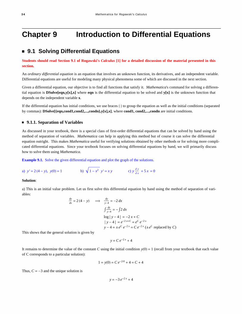
Example 9.1. Solve the given differential equation and plot the graph of the solutions.
a) y ' = 2 4 - y, y0 = 1 b) 1 - x2 y ' = x y c) yd y
d x+ 5 x = 0
Solution:
a) This is an initial value problem. Let us first solve this differential equation by hand using the method of separation of vari-ables:
dy
dx= 2 4 - y ï
dy
y-4= -2 dx
dy
y-4= - 2 dx
log y - 4 = -2 x + Cy - 4 = e-2 x+C = eC e-2 x
y - 4 = ≤eC e-2 x = C e-2 x (≤eC replaced by C)This shows that the general solution is given by
y = C e-2 x + 4
It remains to determine the value of the constant C using the initial condition y0 = 1 (recall from your textbook that each valueof C corresponds to a particular solution):
1 = y0 = C e-2ÿ0 + 4 = C + 4
Thus, C = -3 and the unique solution is
y = -3 e-2 x + 4
34 Mathematica for Rogawski's Calculus

Next, let us confirm this solution using Mathematica. Recall that when entering a differential equation in Mathematica, we writeyx instead of y to make explicit the dependence on x.
In[147]:= sola DSolvey'x 2 4 yx, yx, xOut[147]= yx 4 2 x C1This solution agrees with the solution obtained earlier by hand (the arbitrary constant C1 is the same to the constant C). We canvisualize the behavior of the particular solutions by plotting some of their graphs for different values of C1. First, let us definethe general solution to be gx, c, where c = C1 as follows (see Section 1.2.3 to learn how to extract elements from lists):
In[148]:= Clearg, x, cgx_, c_ sola1, 1, 2 . C1 c
Out[149]= 4 c 2 x
We then plot the one-parameter family of solution curves by combining the graphs of gx, c for c = -5, -4, ..., 5.
In[150]:= plotgeneralsolution
PlotTablegx, c, c, 5, 5, x, 2, 2, PlotRange 20, 20, ImageSize 250
Out[150]=-2 -1 1 2
-20
-10
10
20
Can you explain how the graph of gx, c varies as c varies? Which c value corresponds to the top graph?
Next, to find the unique particular solution satisfying the given initial condition y0 = 1, we solve the equation g0, c = 1 for c:
In[151]:= Solveg0, c 1, cOut[151]= c 3Thus, our unique solution is y = -3 e-2 x + 4. This agrees with the solution we obtained earlier by hand. Of course, Mathematicacan solve for the unique solution on its own, bypassing the algebraic steps involved:
In[152]:= sola DSolvey'x 2 4 yx, y0 1, yx, xOut[152]= yx 2 x 3 4 2 xHowever, this unique solution does not appear to be the same as the one we obtained earlier. To remedy this, let us extractsolution from the output and define it as y = f x:In[153]:= fx_ sola1, 1, 2Out[153]= 2 x 3 4 2 xWe then apply the Expand command to simplify f x:
Chapter 3 35

In[154]:= ExpandfxOut[154]= 4 3 2 x
Thus, the unique solution obtained by Mathematica is the same as the one obtained by hand. Here is the plot of the uniquesolution:
In[155]:= plotuniquesolution Plotfx, x, 2, 2,
PlotRange 20, 20, PlotStyle Thickness0.01, ImageSize 250
Out[155]=-2 -1 1 2
-20
-10
10
20
Lastly, we combine plots of the general solution and the unique solution to show where the latter (bold graph) is situated in theformer:
In[156]:= Showplotgeneralsolution, plotuniquesolution, ImageSize 250
Out[156]=-2 -1 1 2
-20
-10
10
20
b) From this point on, we shall skip using the method of separation of variables, which we leave for the reader to employ, andproceed directly to solving all differential equations using Mathematica as in part a) above.
In[157]:= solb DSolve 1 x2 y'x x yx, yx, x
Out[157]= yx 1x2C1
Again, we can visualize the behavior of these particular solutions by plotting graphs of some particular solutions correspondingto different values of C1. As before, we define the general solution to be gx, c, where c = C1. In[158]:= Clearg, x, c
gx_, c_ solb1, 1, 2 . C1 c
Out[159]= c 1x2
We then make a combined plot of the graphs of gx, c for c = -5, -4, ..., 5.
36 Mathematica for Rogawski's Calculus

In[160]:= PlotTablegx, c, c, 5, 5, x, 2, 2, ImageSize 250
Out[160]=-2 -1 1 2
-4
-2
2
4
c) We again use Mathematica to directly obtain the solution:
In[161]:= Clearysolde DSolve yx y'x 5 x 0, yx, x
Out[162]= yx 5 x2 2 C1 , yx 5 x2 2 C1
Observe that the two solutions, which we denote by f x, c and gx, c, differ only in sign:
In[163]:= fx_, c_ solde2, 1, 2 . C1 c
gx_, c_ solde1, 1, 2 . C1 c
Out[163]= 2 c 5 x2
Out[164]= 2 c 5 x2
The following two plots show the graphs of f x, c and gx, c corresponding to c = -50, -40, ..., 0, ..., 40, 50.
In[165]:= PlotTablefx, c, c, 50, 50, 10,x, 5, 5, PlotRange 0, 10, ImageSize 250
Out[165]=
-4 -2 0 2 4
2
4
6
8
10
Chapter 3 37

In[166]:= PlotTablegx, c, c, 50, 50, 10,
x, 5, 5, PlotRange 10, 0, ImageSize 250
Out[166]=
-4 -2 2 4
-10
-8
-6
-4
-2
Observe that the two solutions y = - 5 x2 + 2 c and y = 5 x2 + 2 c can be represented by a single equation:
y2 - 5 x2 = 2 c
which describes a family of hyperbolas. Here is a contour plot of this equation. Observe that it nothing more than a combinationof the two plots above as to be expected.
In[167]:= ContourPloty2 5 x2, x, 5, 5, y, 10, 10, Frame False,
Axes True, ContourShading False, Contours 10, ImageSize 250
Out[167]=
ü Exercises
In Exercises 1 through 8, solve the given differential equations. If initial conditions are also given, then plot the unique solution.If not, then make a combine plot of several particular solutions by choosing various values of the arbitrary constant. Thendescribe the graphs and explain how they vary as the arbitrary constant varies.
1. 1 + x2 y ' = x2 y; y0 = 2 2. y ' + 3 x4 y2 = 0; y0 = 1
3. y ' + y2 = -1; y0 = -1 4. y ' + 3 y = sin x; y0 = 0
38 Mathematica for Rogawski's Calculus

5. y ' = -2 x y (bell-shaped curves) 6. 16 y y ' + 9 x = 07. y ' - y = y2 8. 2 x y y ' - y2 + x2 = 0
9. Consider the differential equation
3 + 2 y y ' = 2 - ex, y0 = a
a) Solve the equation.b) Plot the graphs for values of a = -2, -1, 0, 1, 2.c) Plot the graphs for the values of a = -.5, -.1, .1, .5.NOTE: For parts b) and c), make sure to use a sufficiently large interval for x.
10. Consider the differential equation
y = x y b - y 4 + x, y0 = a
a) Solve the equation.b) Plot the graphs for values of a = -2, -1, 0, 1, 2 and b = -2, -1, 0, 1, 2.c) Plot the graphs for the values of a = -.5, -.1, .1, .5 and b = -.5, -.1, .1, .5d) Show that the limit as xØ ¶ of the solution does not depend on a. Does the limit depend on b? If so, how?
11. Suppose a skydiver falls from rest toward the earth and assume that the air resistance caused by his open parachute is propor-tional to the square of his velocity v with proportionality constant k (we neglect air resistance due to the skydiver himself). Amodel for describing the skydiver's velocity after his parachute opens is then given by the differential equation
v ' = - k
mv2 -
m g
k
where m is the mass of the skydiver and g = 9.8 meters/sec2 is his acceleration due to gravity.
a) Solve the equation assuming an initial velocity v0 = v0.b) Suppose that for a particular skydiver m = 70 kg and k = 30 kg meter. Solve the equation again using these values and plot theparticular solutions for the following values of v0: 0, 2, ..., 10.c) What is the skydiver's limiting (terminal) velocity as tض for each of the particular solutions in part b)? Does it depend onv0?d) Find a formula for the terminal velocity in terms of m, g, and k.
12. Recall that the first-order linear differential equation y ' + y = 0 has solution y = C e-x. Solve the following higher-ordergeneralizations of this equation:
a) y '' + 2 y ' + y = 0b) y ''' + 3 y '' + 3 y ' + y = 0c) y4 + 4 y ''' + 6 y '' + 4 y ' + y = 0d) Do you recognize the coefficients involved in the differential equations above? What would be the next differential equation(of order 5) that follows this pattern? Solve this differential equation to verify that its solution follows that same pattern exhibitedin parts a) through c).
ü 9.2 Models of the Form y ' = ky - bStudents should read Section 9.2 of Rogawski's Calculus [1] for a detailed discussion of the material presented in thissection.
NOTE: The differential equations we encounter in this section can be solved by the method of separation of variables and isdiscussed in the text. We leave it to the reader to solve the examples in this section by hand to verify the solutions obtained using
Chapter 3 39

Mathematica.
ü 9.2.1. Bacteria Growth
The growth of bacteria in a culture is known to be proportional to the amount of the bacteria present at time t. Suppose the initialamount of the bacteria is y0 and the amount at time t is yt. Then the above physical law is modeled by the differential equation
y ' = k y, y0 = y0
where k is the proportionality (growth) constant. Such a model exhibits exponential growth as can be seen from its solution below:
In[168]:= ClearkDSolvey'x k yx, y0 y0, yx, x
Out[169]= yx k x y0NOTE: Since the bacteria is growing in number, yt is increasing and hence y ' t > 0. Thus, k must be a positive number.
Example 9.2. Suppose the amount of bacteria in a culture was 200 at time t = 0. It was found that there were 450 bacteria after 2minutes.a) Find the amount of the bacteria at any time t.
b) At what time will the number of bacteria exceed 10,000?
Solution:
a) First, note that y0 = 200 and y2 = 450. We solve the differential equation y ' = k y with the former as the initial condition:
In[170]:= Cleary, t, ksolde DSolvey't k yt, y0 200, yt, t
Out[171]= yt 200 k tIn[172]:= ft_ solde1, 1, 2Out[172]= 200 k t
To find the value of k we solve f 2 = 450 for k.
In[173]:= solk Solvef2 450, kSolve::ifun : Inverse functions are being used by Solve, so
some solutions may not be found; use Reduce for complete solution information. à
Out[173]= k 1
2Log 9
4
In[174]:= NOut[174]= k 0.405465
Thus, the proportionality constant is k = 1
2l n9 4 º 0.405465. Substituting this value into yt, we see that the amount of
bacteria at a given time t is
yt = 200 e0.405465 t
b) To find the amount of time it takes for the bacteria to exceed 10,000, we solve
40 Mathematica for Rogawski's Calculus

In[175]:= k solk1, 1, 2Solveft 10 000, t
Out[175]=1
2Log 9
4
Solve::ifun : Inverse functions are being used by Solve, sosome solutions may not be found; use Reduce for complete solution information. à
Out[176]= t Log50
Log2 Log3
We can approximate this value for t by
In[177]:= NOut[177]= t 9.64824Thus, it takes about 9.64824 minutes for the bacteria to reach 10,000. To visually see this, we plot the graphs of the solutionyt = 200 e0.405465 t (blue curve) and y = 10 000 (red line) on the same axes.
In[178]:= Plotft, 10 000, t, 0, 15, PlotStyle Blue, Red, ImageSize 250
Out[178]=
2 4 6 8 10 12 14
5000
10 000
15 000
20 000
NOTE: The solution yt = 200 e0.405465 t is only approximate since we approximated the growth constant k. By using the exact
value for k = 1
2l n9 4 = l n3 2, we can derive the exact solution:
yt = 200 ek t = 200 e t ln3
2 = 200 e ln 3
2t
= 200 3
2t
This agrees with the answer obtained by Mathematica:
In[179]:= ftOut[179]= 25 23t 3t
ü 9.2.2. Radioactive Decay
The differential equation y ' = k y is also used to model the amount of a radioactive substance whose rate of decay is proportionalto the amount present. However, in this case we note that the proportionality constant k < 0. (Explain this!)
Example 9.3. Carbon dating is a method used to determine the age of a fossil based on the amount of radioactive Carbon-14 in itcompared to the amount normally found in the living environment. Suppose that a bone fossil contains 5% of the amount ofCarbon-14 normally found in living animals. If the half-life of Carbon-14 is 5600 years, estimate the age of the bone.
Solution: Let yt) be the amount of Carbon-14 in the bone and let y0 be the initial amount of Carbon-14. Then the differentialequation we need to solve is
Chapter 3 41

In[180]:= Cleark, y, y0solde DSolvey't k yt, y0 y0 , yt, t
Out[181]= yt k t y0
Thus, the solution to the differential equation is yt = y0 ek t. The half-life of Carbon-14 is 5600 implies that y5600 = 1
2y0. We
solve this equation for k:
In[182]:= yt_ solde1, 1, 2solk Solvey5600
1
2y0, k
Out[182]= k t y0
Solve::ifun : Inverse functions are being used by Solve, so
some solutions may not be found; use Reduce for complete solution information. à
Out[183]= k Log2
5600
In[184]:= NOut[184]= k 0.000123776Thus, k = -0.000123776. To find the age of the bone, we solve y t = 0.05 y0 (5% of the initial amount) for t.
In[185]:= k Log2
5600;
Solveyt 0.05 y0, tSolve::ifun : Inverse functions are being used by Solve, so
some solutions may not be found; use Reduce for complete solution information. à
Out[186]= t 24 202.8Thus, the bone is about 24,203 years old. Observe that it not necessary to know the original amount y0 of Carbon-14 in the bone.
ü 9.2.3. Annuity
An annuity is an investment in which a principal amount of money is placed in a bank account that earns interest at an annualrate (compounded continuously) and the money is withdrawn at a regular interval. The differential equation that models anannuity is given by the annuity equation (rate of change = growth due to interest - withdrawal rate):
P ' t = r Pt -W = rPt - W
r
where Pt is the balance in the annuity at time t, r is the interest rate, and W is the rate (dollars per year) at which money iswithdrawn continuously.
Example 9.4. Find the general solution of the annuity equation for Pt and then use it to calculate the following:a) Assume r = 6% and W = $ 6000 per year and P0 = $ 50 000. Find Pt and determine if and when the annuity runs out ofmoney.b) Assume r = 6% and W = $ 6000 per year and P0 = $ 100 000. Find Pt and determine if and when the annuity runs out ofmoney.c) Assume r = 6% and W = $ 12 000 per year. If we want the annuity to run out of money after 20 years, how much should be
42 Mathematica for Rogawski's Calculus

invested now?
Solution: We solve
In[187]:= DSolveP't r Pt W
r, Pt, t
Out[187]= Pt W
r r t C1
Thus, the general solution is Pt =W r + c er t.
a) We set r = 0.06, W = 6000, and solve the initial value problem:
In[188]:= Clearr, W, Pr 0.06;W 6000;
solde DSolveP't r Pt W
r, P0 50 000, Pt, t
Out[191]= Pt 100 000. 50 000. 0.06 t We then define Pt to be the solution above and plot it to see when the money will run out.
In[192]:= Pt_ solde1, 1, 2PlotPt, t, 0, 15, ImageSize 250
Out[192]= 100 000. 50 000. 0.06 t
Out[193]=
2 4 6 8 10 12 14
-20 000
-10 000
10 000
20 000
30 000
40 000
50 000
As the graph indicates, the money runs out after approximately 11.5 years. We can confirm this by solving Pt = 0:
In[194]:= NSolvePt 0, tNSolve::ifun : Inverse functions are being used by NSolve, so
some solutions may not be found; use Reduce for complete solution information. à
Out[194]= t 11.5525b) We repeat the procedure in part a) with the obvious modifications:
Chapter 3 43

In[195]:= Clearr, W, Pr 0.06;W 6000;
solde DSolveP't r Pt W
r, P0 100 000, Pt, t;
Pt_ solde1, 1, 2PlotPt, t, 0, 80, ImageSize 250
Out[199]= 100 000.
Out[200]=
20 40 60 80
50 000
100 000
150 000
200 000
Observe that the balance Pt = 100, 000 remains constant (can you explain why?) and thus the account will never run out ofmoney. What happens if we invest $100,001? $99,999?
c) In this case, we have r = 0.06 and W = 10 000 per year. The general solution is then given by
In[201]:= Clearr, W, P, cr 0.06;W 12 000;
dsol DSolveP't r Pt W
r, P0 c, Pt, t;
Pt_ dsol1, 1, 2Out[205]= 200 000. 200 000. 0.06 t 1. c 0.06 t
To determine the principal amount that will make the account run out of money in 20 years, we solve P20 = 0 for c:
In[206]:= NSolveP20 0, cOut[206]= c 139 761.Thus, we need to invest $139,761.00 now.
ü 9.2.4. Newton's Law of Cooling
Newton's Law of Cooling states that the rate of change in the temperature of an object is proportional to the difference between itstemperature and that of the surrounding environment (known as the ambient temperature). If A is the ambient temperature andTt is the temperature of the object at time t, then the differential equation that models this law is
T ' t = -kTt - A, T0 = T0
where T0 is the initial temperature of the object and k is a positive proportionality constant.
Example 9.6. The temperature in an oven is 350° F when the oven is turned off. After 15 minutes, the temperature is 250° F.
44 Mathematica for Rogawski's Calculus
Assume the temperature in the house is 70° F.
a) Find the temperature of the oven at any time t.
b) At what time will the temperature become 75° F? c) What will the temperature be in the limit as tØ ¶?d) Does your answer in c) conform with your physical intuition?
Solution:
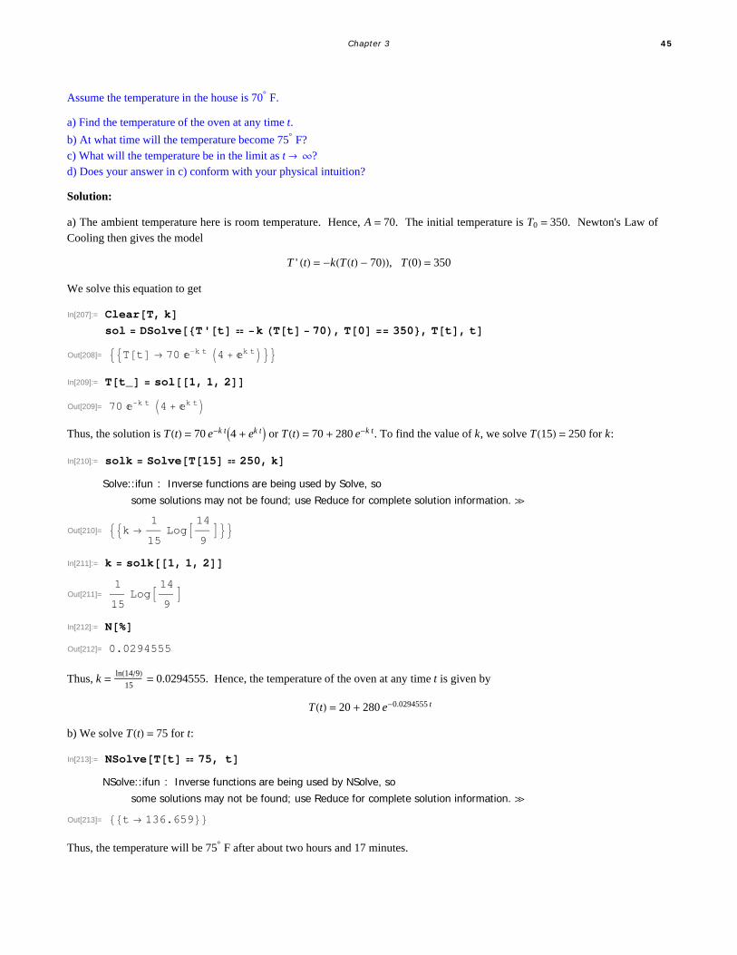
a) The ambient temperature here is room temperature. Hence, A = 70. The initial temperature is T0 = 350. Newton's Law ofCooling then gives the model
T ' t = -kTt - 70, T0 = 350
We solve this equation to get
In[207]:= ClearT, ksol DSolveT't k Tt 70, T0 350, Tt, t
Out[208]= Tt 70 k t 4 k tIn[209]:= Tt_ sol1, 1, 2Out[209]= 70 k t 4 k tThus, the solution is Tt = 70 e-k t4 + ek t or Tt = 70 + 280 e-k t. To find the value of k, we solve T15 = 250 for k:
In[210]:= solk SolveT15 250, kSolve::ifun : Inverse functions are being used by Solve, so
some solutions may not be found; use Reduce for complete solution information. à
Out[210]= k 1
15Log 14
9
In[211]:= k solk1, 1, 2
Out[211]=1
15Log 14
9
In[212]:= NOut[212]= 0.0294555
Thus, k = ln14915
= 0.0294555. Hence, the temperature of the oven at any time t is given by
Tt = 20 + 280 e-0.0294555 t
b) We solve Tt = 75 for t:
In[213]:= NSolveTt 75, tNSolve::ifun : Inverse functions are being used by NSolve, so
some solutions may not be found; use Reduce for complete solution information. à
Out[213]= t 136.659Thus, the temperature will be 75° F after about two hours and 17 minutes.
Chapter 3 45

c) We make a plot of the solution:
In[214]:= PlotTt, t, 0, 100, AxesOrigin 0, 0, ImageSize 250
Out[214]=
20 40 60 80 100
50
100
150
200
250
300
350
To find the limiting temperature, we evaluate
In[215]:= LimitTt, t InfinityOut[215]= 70
d) Since heat flows from a region of higher temperature to a region of lower temperature, it is intuitively clear that the oven will
cool down to the room (ambient) temperature. Hence, the limit should be 70° F as expected.
ü Exercises
1. Mass of bacteria in a culture grow at a rate proportional to its size. Suppose the culture contains 200 cells intially and there are800 cells after 3 hours.
a) Find the formula for the number of cells in the culture at time t.b) Find the amount of bacteria after 2 hours.c) At what time will the bacteria exceed 10,000 cells?
2. A mummy excavated from an archaelogical site in Egypt is found to contain 20% of Carbon-14 normally found in livinghumans. Use carbon dating to estimate the age of the mummy.
3. Plutonium-239 is a highly radioactive element generated from waste in nuclear power plants and has a half-life of approxi-mately 24,000 years. How many years would it take for Plutonium-239 to decay to a safe level of 1/1000 its original amount?
4. Solve the following using the annuity differential eqaution discussed in this section.a) Assume r = 6% and W = $500 per year and P0 = $5, 000. Find Pt and determine when the annuity runs out of money.b) Assume r = 6% and W = $500 per year and P0 = $9, 000. Find Pt and determine when the annuity runs out of money.c) Assume r = 6% and W = $20, 000 per year. If we want the annuity to run out after 40 years, how much should we investnow?
5. Suppose a retired worker wants to invest in an annuity that will pay out $10,000 per year.a) Assuming the annuity has an interest rate of 5%, find the minimum principal amount that should be invested so that the annuitynever runs out of money.b) Assuming the principal amount of money invested is $250,000, find the minimum interest rate that the annuity should bear sothat it never runs out of money.
6. A hot metal rod is placed in a water bath whose temperature is 40° F. The rod cools from 300° F to 200° F in 1 minute. Howlong will take the rood to cool down to 150° F? 45° F?
46 Mathematica for Rogawski's Calculus

ü 9.3 Numerical Methods Using Slope Fields
Students should read Section 9.3 of Rogawski's Calculus [1] for a detailed discussion of the material presented in thissection.
ü 9.3.1. Slope Fields
Consider a differential equation in the form
y ' = f x, ySince y ' represents the slope of the line tangent to the graph of the solution y, we can think of f x, y as the slope of the sametangent line at the point x, y, which we indicate by drawing a segment of it at the point of tangency. The set of all such linesegments (normalized to have the same length) is called the slope (or direction) field of the differential equation. Note that theslope field gives a graphical approximation to the solution. It enables us to draw or visualize the graph of the unique solution ofthe equation passing through a given point. We will illustrate this in an upcoming example.
To plot the slope field of the differential equation y ' = f x, y along the intervals a, b and c, d on the x- and y-axis, respec-
tively, we use the command VectorPlot[{1, f[x, y]}, {x, a, b}, {y, c, d}], where slope is represented as a two-dimensional vector1, f x, y with the change in x normalized to equal 1.
NOTE: The command VectorPlot replaces the command VectorFieldPlot, which is obsolete in version 7 of Mathematica.
Example 9.9. Consider the differential equation y ' = x2 - 2 y, y0 = -1.
a) Draw the slope fields for the differential equation.b) Solve the differential equation.c) Plot both the slope field and the solution on the same axes.d) Redo parts b) and c) for the same equation but with initial condition given by ya = b. Choose various values for a and b.
Solution:
a) Here, f x, y = x2 - 2 y. We use the VectorPlot command to plot the corresponding slope field:
In[216]:= fx_, y_ : x2 2 y
Chapter 3 47

In[217]:= plot1 VectorPlot1, fx, y, x, 5, 5, y, 10, 10, Axes True,
Frame False, VectorScale Tiny, Tiny, None, ImageSize 250
Out[217]=-4 -2 2 4
-10
-5
5
10
b) We use the DSolve command to find the exact solution of the differential equation.
In[218]:= Cleary, x, gsol DSolvey'x fx, yx, y0 1, yx, xgx_ sol1, 1, 2
Out[219]= yx 1
42 x 5 2 x 2 2 x x 2 2 x x2
Out[220]=1
42 x 5 2 x 2 2 x x 2 2 x x2
c) We now plot the slope field together with the solution above passing through the point 0, -1:In[221]:= plot2 Plotgx, x, 5, 5, PlotRange 10, 10, ImageSize 250
Out[221]=-4 -2 2 4
-10
-5
5
10
48 Mathematica for Rogawski's Calculus

In[222]:= Showplot1, plot2, GraphicsPointSizeLarge, Point0, 1, ImageSize 250
Out[222]=-4 -2 2 4
-10
-5
5
10
d) We can show several graphs of solution curves (called integral curves) together with the corresponding slope field. Here is anexample of how this can be done.
In[223]:= Cleary, x, h, a, bsola DSolvey'x fx, yx, ya b, yx, x;hx_, a_, b_ Simplifysola1, 1, 2
Out[225]=1
42 x 1 2 a 2 a2 4 b 2 a 2 x 1 2 x 2 x2
In[226]:= plot3 PlotEvaluateTablehx, a, b, a, 3, 3, 2, b, 3, 3, 2,x, 5, 5, PlotRange 10, 10;
Showplot1, plot3, ImageSize 250
Out[227]=-4 -2 2 4
-10
-5
5
10
Chapter 3 49

ü 9.3.2. Euler's Method
The simplest numerical method for solving a first order differential equation is Euler's Method. This method approximates thesolution by moving along tangent lines described by the slope field of the differential equation. Here is a brief description.
Let y = fx be the solution of the differential equation
y ' = f x, y, yx0 = y0
Then the equation of the line tangent to the graph of y = jx at x = x0 is given by
y = j ' x0 x - x0 + jx0But when x = x0, we have jt0 = y0 and j ' x0 = f x0, y0. Thus, when x is close to x0, jx can be approximated by
y º f x0, y0 x - x0 + y0
We now choose h > 0 to be a small positive number, called the step size, and define x1 = x0 + h. Then jx1 is approximatelyequal to
y1 = y0 + f x0, y0 x1 - x0or
y1 = y0 + h f x0, y0We repeat the above argument at the point x1, y1 to get an approximation of jx2, where x2 = x1 + h = x0 + 2 h:
y2 = y1 + h f x1, y1Proceeding in this manner, we obtain Euler's Method:
yn+1 = yn + h f xn, yn for n = 0, 1, 2, 3, ....
where jxn º yn.
If the approximated solution is calculated over an interval a, b and the step size h is specified, then the number of iterations (orsteps) required is given by m = b - a h, where x0 = a and xn = x0 + n h.
Here is a Mathematica program called Euler for evaluating Euler's Method in m steps (the option SetPrecision sets the precisionof our calculations to 10 digits).
In[228]:= Clearf, x, y, x0, y0, h, mEulerf_, h_, m_ : Modulen,
Doyn 1 SetPrecisionNyn h fxn, yn, 10;xn 1 xn h,n, 0, m
Example 9.7. Use the Euler program to construct a table of solution values for the differential equation y ' = x2 + 2 y, y0 = 1with a step size of h = 0.1 and for m = 10 steps.
Solution: Here f x, y = x2 + 2 y, x0 = 0, y0 = 1.
50 Mathematica for Rogawski's Calculus
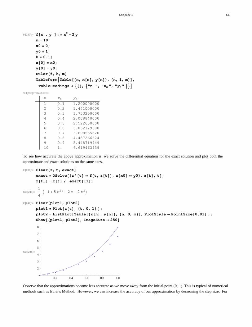
In[230]:= fx_, y_ : x2 2 y
m 10;x0 0;y0 1;h 0.1;
x0 x0;y0 y0;Eulerf, h, mTableFormTablen, xn, yn, n, 1, m,
TableHeadings , "n ", "xn ", "yn " Out[238]//TableForm=
n xn yn
1 0.1 1.2000000002 0.2 1.4410000003 0.3 1.7332000004 0.4 2.0888400005 0.5 2.5226080006 0.6 3.0521296007 0.7 3.6985555208 0.8 4.4872666249 0.9 5.44871994910 1. 6.619463939
To see how accurate the above approximation is, we solve the differential equation for the exact solution and plot both theapproximate and exact solutions on the same axes.
In[239]:= Clearz, t, exactexact DSolvez't ft, zt, zx0 y0, zt, t;zt_ zt . exact1
Out[241]=1
41 5 2 t 2 t 2 t2
In[242]:= Clearplot1, plot2plot1 Plotzt, t, 0, 1 ;plot2 ListPlotTablexn, yn, n, 0, m, PlotStyle PointSize0.01 ;
Showplot1, plot2, ImageSize 250
Out[245]=
0.2 0.4 0.6 0.8 1.0
2
3
4
5
6
7
8
Observe that the approximations become less accurate as we move away from the initial point 0, 1. This is typical of numericalmethods such as Euler's Method. However, we can increase the accuracy of our approximation by decreasing the step size. For
Chapter 3 51

example, we recompute the solution using h = 0.05 (this increases the number of steps to m = 20):
In[246]:= h 0.05;m 20;Eulerf, h, mTableFormTablen, xn, yn, n, 1, m,
TableHeadings , "n ", "xn ", "yn " Out[249]//TableForm=
n xn yn
1 0.05 1.1000000002 0.1 1.2101250003 0.15 1.3316375004 0.2 1.4659262505 0.25 1.6145188756 0.3 1.7790957637 0.35 1.9615053398 0.4 2.1637808739 0.45 2.38815896010 0.5 2.63709985611 0.55 2.91330984112 0.6 3.21976582613 0.65 3.55974240814 0.7 3.93684164915 0.75 4.35502581416 0.8 4.81865339517 0.85 5.33251873518 0.9 5.90189560819 0.95 6.53258516920 1. 7.230968686
The following plot of the two numerical solutions corresponding to h = 0.1 (small blue dots) and h = 0.05 (large red dots) clearlyshows that the latter is more accurate in comparison to the exact solution (curve):
In[250]:= plot3 ListPlotTablexn, yn, n, 0, m,PlotStyle PointSize0.01, Red, PointSize0.015 ;
Showplot1, plot2, plot3, ImageSize 250
Out[251]=
0.2 0.4 0.6 0.8 1.0
2
3
4
5
6
7
8
Here is a modification of the Euler progam that allows the user to input the endpoints a and b directly (instead of the step size h)and m.
52 Mathematica for Rogawski's Calculus
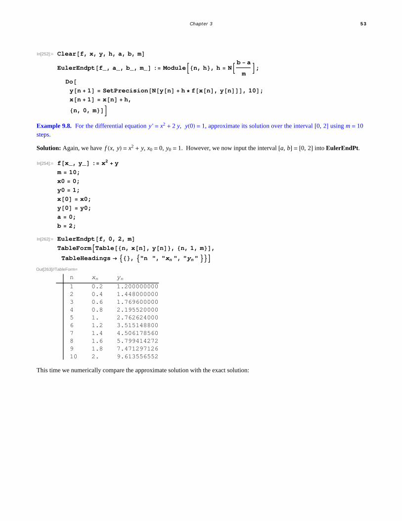
In[252]:= Clearf, x, y, h, a, b, mEulerEndptf_, a_, b_, m_ : Modulen, h, h N b a
m;
Doyn 1 SetPrecisionNyn h fxn, yn, 10;xn 1 xn h,
n, 0, mExample 9.8. For the differential equation y ' = x2 + 2 y, y0 = 1, approximate its solution over the interval 0, 2 using m = 10steps.
Solution: Again, we have f x, y = x2 + y, x0 = 0, y0 = 1. However, we now input the interval a, b = 0, 2 into EulerEndPt.
In[254]:= fx_, y_ : x2 y
m 10;x0 0;y0 1;
x0 x0;y0 y0;a 0;b 2;
In[262]:= EulerEndptf, 0, 2, mTableFormTablen, xn, yn, n, 1, m,
TableHeadings , "n ", "xn ", "yn " Out[263]//TableForm=
n xn yn
1 0.2 1.2000000002 0.4 1.4480000003 0.6 1.7696000004 0.8 2.1955200005 1. 2.7626240006 1.2 3.5151488007 1.4 4.5061785608 1.6 5.7994142729 1.8 7.47129712610 2. 9.613556552
This time we numerically compare the approximate solution with the exact solution:
Chapter 3 53

In[264]:= Clearz, t, exactexact DSolvez't ft, zt, zx0 y0, zt, t;zt_ zt . exact1TableFormTablen, xn, yn, Nzx0 n b a m, n, 1, m,
TableHeadings , "n ", "xn ", "yn ", "yn" Out[266]= 2 3 t 2 t t2
Out[267]//TableForm=
n xn yn yn1 0.2 1.200000000 1.224212 0.4 1.448000000 1.515473 0.6 1.769600000 1.906364 0.8 2.195520000 2.436625 1. 2.762624000 3.154856 1.2 3.515148800 4.120357 1.4 4.506178560 5.40568 1.6 5.799414272 7.09919 1.8 7.471297126 9.3089410 2. 9.613556552 12.1672
ü Exercises
In Exercises 1 through 4, plot the slope field of the given differential equations:1. y ' = x2 + y2 2. y ' = t2 y 3. y ' = sinx + y 4. y ' = x e-y
5. Consider the differential equation y ' = 3 y - 2 y2.a) Draw the slope field for the differential equation.b) Solve the differential equation.c) Assume y0 = 2. Plot the graph of the solution for this case and also the slope field on the same axes. Discuss the behavior ofthe solution as xض.d) Redo part c) for the same differential equation but with initial condition given by ya = b (choose various values for a and b).
In Exercises 6 through 9, use Euler's Method to find a numerical solution to the given initial value problem along the statedinterval and using the prescribed number of steps. Also, find their exact solutions and compare the results.6. y ' = x2 - y, y0 = 1; 0, 1; m = 10 7. y ' = 1 - x2 cos y, y1 = 0; 1, 2; m = 208. y ' - y2 = x, y0 = 1; 0, 5;m = 50 9. y ' = -3 x 2 + lnx2 + y, y1 = 1; 1, 2; m = 100
10. Heun's method is a numerical method that improves on Euler's method. It uses the approximation from Euler's method as anauxiliary value (called a predictor), which we denote by yn+1
* :
yn+1* = yn + h f xn, yn
The actual approximation (called the corrector) is then computed as the mean of yn+1* (based on the slope of the tangent line at
xn, yn) and yn+1** = yn + h f xn+1, yn+1
* (based on the slope of the tangent line at xn+1, yn+1* ):
yn+1 =1
2yn+1* + yn+1
** = yn +1
2h f xn, yn + h f xn+1, yn+1
* a) Apply Heun's method to Exercise 6 and the compare the results obtained by Euler's method with the exact solution. Howmuch more accurate is Heun's method?b) Redo part a) using m = 20. How much more accurate is the solution compared to that for m = 10?
54 Mathematica for Rogawski's Calculus
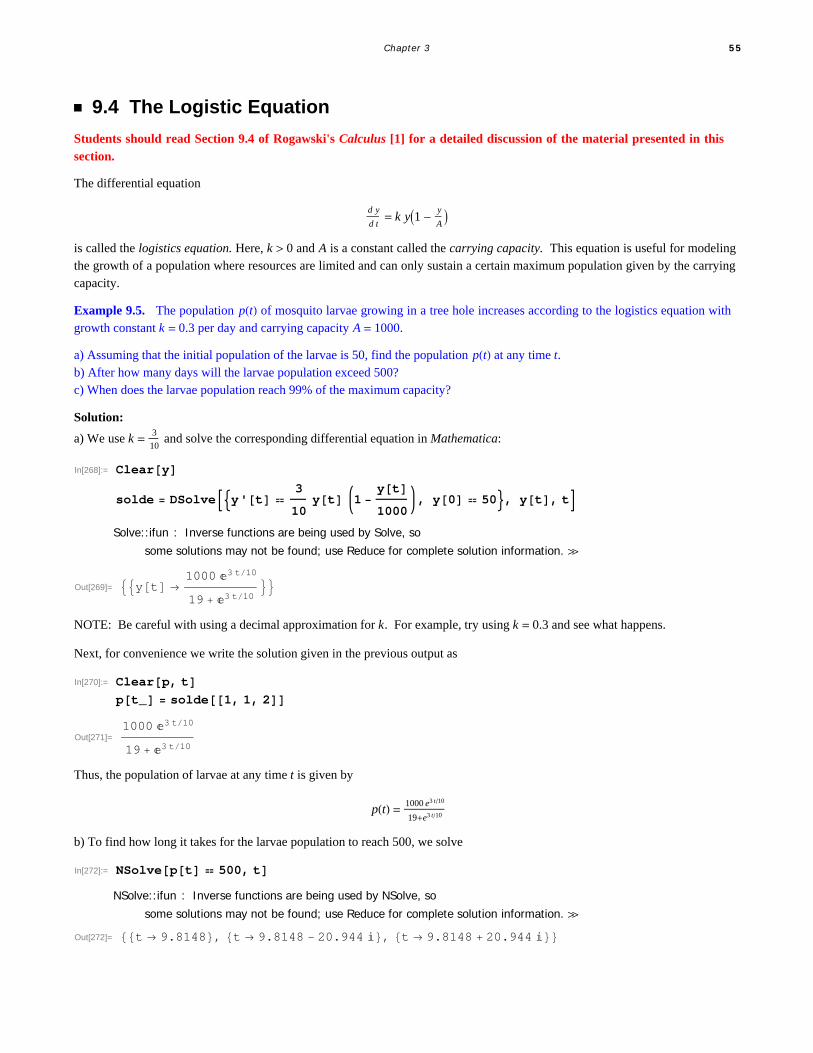
ü 9.4 The Logistic Equation
Students should read Section 9.4 of Rogawski's Calculus [1] for a detailed discussion of the material presented in thissection.
The differential equation
d y
d t= k y1 - y
A
is called the logistics equation. Here, k > 0 and A is a constant called the carrying capacity. This equation is useful for modelingthe growth of a population where resources are limited and can only sustain a certain maximum population given by the carryingcapacity.
Example 9.5. The population pt of mosquito larvae growing in a tree hole increases according to the logistics equation withgrowth constant k = 0.3 per day and carrying capacity A = 1000.
a) Assuming that the initial population of the larvae is 50, find the population pt at any time t. b) After how many days will the larvae population exceed 500?c) When does the larvae population reach 99% of the maximum capacity?
Solution:
a) We use k = 3
10 and solve the corresponding differential equation in Mathematica:
In[268]:= Clearysolde DSolvey't
3
10yt 1
yt1000
, y0 50, yt, t
Solve::ifun : Inverse functions are being used by Solve, so
some solutions may not be found; use Reduce for complete solution information. à
Out[269]= yt 1000 3 t10
19 3 t10
NOTE: Be careful with using a decimal approximation for k. For example, try using k = 0.3 and see what happens.
Next, for convenience we write the solution given in the previous output as
In[270]:= Clearp, tpt_ solde1, 1, 2
Out[271]=1000 3 t10
19 3 t10
Thus, the population of larvae at any time t is given by
pt = 1000 e3 t10
19+e3 t10
b) To find how long it takes for the larvae population to reach 500, we solve
In[272]:= NSolvept 500, tNSolve::ifun : Inverse functions are being used by NSolve, so
some solutions may not be found; use Reduce for complete solution information. à
Out[272]= t 9.8148, t 9.8148 20.944 , t 9.8148 20.944
Chapter 3 55

Thus, it takes about ten days for the larvae population to exceed 500. Observe that p10 º 513.887.
NOTE: We ignored the other two solutions in the previous output since they are complex-valued and not physically relevant.
c) We first plot the graph of pt to estimate the number of days required for the larvae population to reach 99% of the maximumcapacity, that is, pt = 999.
In[273]:= Plotpt, t, 0, 60, ImageSize 250
Out[273]=
10 20 30 40 50 60
200
400
600
800
1000
It appears that the population reaches 999 larvae after t = 30. We use the Table command to numerically confirm this.
In[274]:= TableFormTablet, Npt, 20, t, 10, 50, 5,TableHeadings , "Days ", "Larvae Population"
Out[274]//TableForm=
Days Larvae Population10 513.8866830116854318815 825.7154653278878200720 955.0220053824840431625 989.6006793002358551430 997.6606988835103176735 999.4770810496474217340 999.8832735919316938645 999.9739524558509316550 999.99418788969128789
We can reasonably conclude from the table that the population reaches 999 larvae between 30 and 35 days. To obtain a moreprecise answer, we use Mathematica to solve pt = 999 for t:
In[275]:= NSolvept 999, tNSolve::ifun : Inverse functions are being used by NSolve, so
some solutions may not be found; use Reduce for complete solution information. à
Out[275]= t 32.8373, t 32.8373 20.944 , t 32.8373 20.944 Thus, the desired time is approximately t = 33 days.
ü Exercises
1. A population of squirrels live in a forest with a carrying capacity of 3000. Assume logistic growth with growth constant k = 0.8per year.a) Find the population of the squirrels at any time t assuming an initial population of P0 = 800.b) How long will it take for the squirrel population to double? Triple?
56 Mathematica for Rogawski's Calculus

2. From 1960 to 2000, the world's population doubled from approximately 3 billion to 6 billion people. Assuming that the humanpopulation follows logistic growth and that the earth has a carrying capacity of 100 billion people, determine the following:a) Find the population at any time t. What is the growth constant?b) What will the population be in the year 2050? How does this answer compare with projections from the United Nations?c) Find the year in which the human population will reach half its carrying capacity?d) When will the population grow the fastest, that is, the point on the graph where it changes from concave up to concave down(point of inflection)? What is the growth rate then?
3. In medicine, the logistics equation is used to model the growth of tumors in certain organs. Suppose a patient is diagnosedwith a tumor that has doubled in size to 2% of his liver when a year ago it only covered 1% of his liver. How long will it take thetumor to grow to 10% of his liver when a transplant will most like by required to increase his chances of survival.
4. The current population of a herd of bison living inside a national park is 1000. To ensure that the population does not reachmore than 1500 bison in 50 years time and 2000 bison in 100 years time, what carrying capacity should the park maintain?Assume that the bison population follows a logistics model.
Chapter 3 57

Chapter 10 Infinite Series
ü 10.1 Sequences
Students should read Section 10.1 of Rogawski’s Calculus [1] for a detailed discussion of the material presented in thissection.
Recall that a sequence is a function whose domain is the set of non-negative integers.
In Mathematica, we denote a sequence an as a function. Thus, instead of an we write an. The limit of a sequence is evaluated by
using the Limit command. When Limit[a[n], nƕ] is evaluated, Mathematica automatically assumes that n is a continuousvariable (instead of a discrete variable). It employs various techniques to evaluate limits.
To plot the graph of a sequence, we use the ListPlot command. ListPlot[list] plots the graph of list, where list is a list of points
x, y, denoted in Mathematica by {x,y}. In our case, list will be the table of values of the form {n,a[n]}. The corresponding plot
command in this case would be ListPlot[Table[{n,a[n]},{n,min,max}].
Example 10.1. Consider the sequence defined by
an =4 n+1
3 n+2
a) Find the first few terms of the sequence.
b) Plot the graph of the sequence.
c) Make a conjecture for the limit based on the graph.
d) Find the limit of the sequence.
Solution:
a) We define the sequence as a function of n and use the Table command to generate the first ten terms of the sequence.
In[276]:= Cleara, nan_ :
4 n 1
3 n 2
58 Mathematica for Rogawski's Calculus

In[278]:= TableFormTablen, an, n, 1, 10,
TableHeadings , "n", "an "Out[278]//TableForm=
n an
1 1
2 98
3 1311
4 1714
5 2117
6 54
7 2923
8 3326
9 3729
10 4132
To obtain decimal expressions of these values, we evaluate
In[279]:= TableFormNTablen, an, n, 1, 10,
TableHeadings , "n", "an "Out[279]//TableForm=
n an
1. 1.2. 1.1253. 1.181824. 1.214295. 1.235296. 1.257. 1.260878. 1.269239. 1.2758610. 1.28125
b) To plot the graph of the sequence, we use the ListPlot command. Here is a plot of the first 100 terms of the sequence.
Chapter 4 59

In[280]:= ListPlotTablen, an, n, 1, 100
Out[280]=
20 40 60 80 100
1.28
1.29
1.30
1.31
1.32
c) The graph suggests that the limit is 1.333 .... We can use the Table command to see this more clearly.
In[281]:= TableFormNTablen, an, n, 1000, 10 000, 1000,
TableHeadings , "n", "an "Out[281]//TableForm=
n an
1000. 1.332782000. 1.333063000. 1.333154000. 1.333195000. 1.333226000. 1.333247000. 1.333258000. 1.333269000. 1.3332710 000. 1.33328
Hence, the limit seems to be 1.3333... or 4/3. Here is a plot of y = 4 3 and the graph of the sequence for large values of n:
60 Mathematica for Rogawski's Calculus
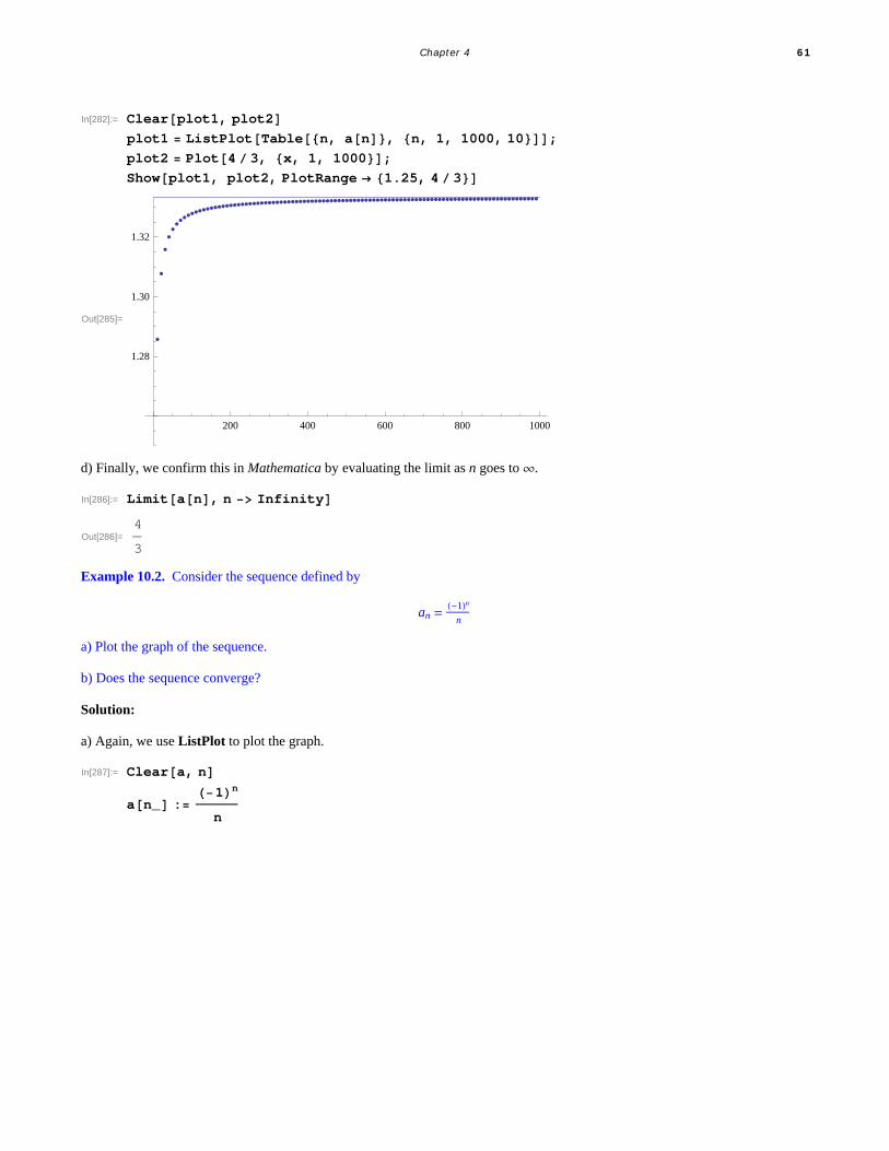
In[282]:= Clearplot1, plot2plot1 ListPlotTablen, an, n, 1, 1000, 10;plot2 Plot4 3, x, 1, 1000;Showplot1, plot2, PlotRange 1.25, 4 3
Out[285]=
200 400 600 800 1000
1.28
1.30
1.32
d) Finally, we confirm this in Mathematica by evaluating the limit as n goes to ¶.
In[286]:= Limitan, n Infinity
Out[286]=4
3
Example 10.2. Consider the sequence defined by
an =-1n
n
a) Plot the graph of the sequence.
b) Does the sequence converge?
Solution:
a) Again, we use ListPlot to plot the graph.
In[287]:= Cleara, nan_ :
1n
n
Chapter 4 61
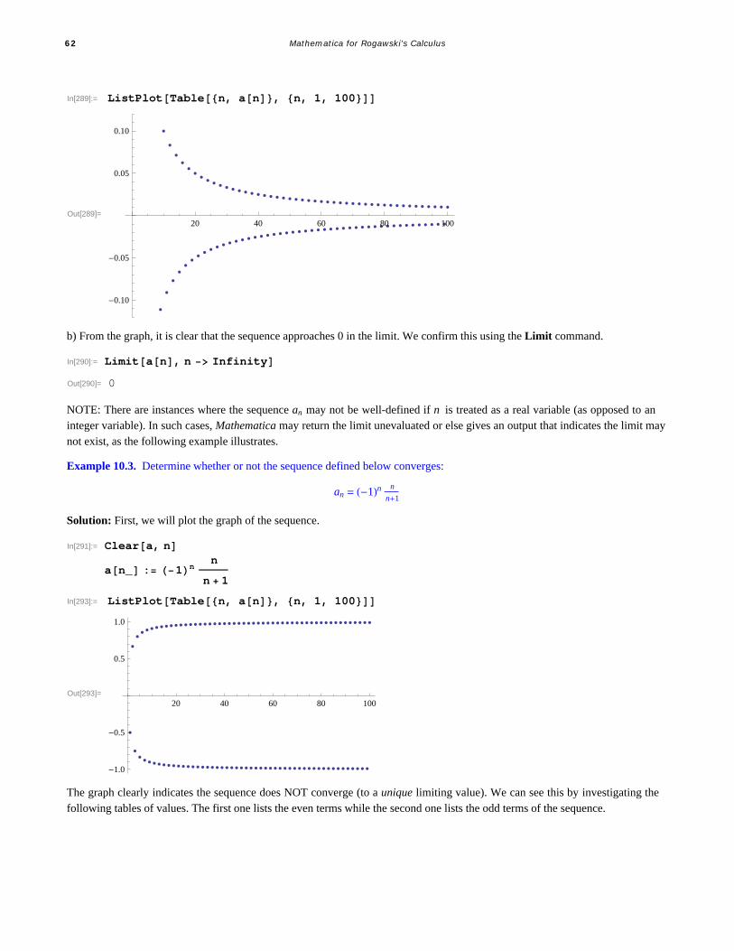
In[289]:= ListPlotTablen, an, n, 1, 100
Out[289]=20 40 60 80 100
-0.10
-0.05
0.05
0.10
b) From the graph, it is clear that the sequence approaches 0 in the limit. We confirm this using the Limit command.
In[290]:= Limitan, n InfinityOut[290]= 0
NOTE: There are instances where the sequence an may not be well-defined if n is treated as a real variable (as opposed to aninteger variable). In such cases, Mathematica may return the limit unevaluated or else gives an output that indicates the limit maynot exist, as the following example illustrates.
Example 10.3. Determine whether or not the sequence defined below converges:
an = -1n n
n+1
Solution: First, we will plot the graph of the sequence.
In[291]:= Cleara, nan_ : 1n
n
n 1
In[293]:= ListPlotTablen, an, n, 1, 100
Out[293]=20 40 60 80 100
-1.0
-0.5
0.5
1.0
The graph clearly indicates the sequence does NOT converge (to a unique limiting value). We can see this by investigating thefollowing tables of values. The first one lists the even terms while the second one lists the odd terms of the sequence.
62 Mathematica for Rogawski's Calculus

In[294]:= TableFormTablen, Na2 n, n, 10, 100, 10,
TableHeadings , "n", "a2n "Out[294]//TableForm=
n a2n
10 0.95238120 0.9756130 0.98360740 0.98765450 0.99009960 0.99173670 0.99290880 0.99378990 0.994475100 0.995025
In[295]:= TableFormTablen, Na2 n 1, n, 10, 100, 10,
TableHeadings , "n", "a2n1 "Out[295]//TableForm=
n a2n1
10 0.9520 0.97530 0.98333340 0.987550 0.9960 0.99166770 0.99285780 0.9937590 0.994444100 0.995
Finally, let us evaluate the limit.
In[296]:= Limitan, n InfinityOut[296]= 2 Interval0,
This output, specifically the notation Interval[{0, p}], means that the limit does not exist uniquely, but has subsequences whose
limits take on the set of complex values e2 i x for all x œ 0, p. This is because the variable n that appears in the Limit command
is automatically assumed by Mathematica to be a complex variable. In our case, for n an integer variable, we have two subse-quences, a2 n and a2 n+1 (even and odd, respectively), converging to different limits (1 and -1, respectively). Thus, an diverges.
Example 10.4. Consider the sequence an defined recursively by a1 = 1 and an+1 = an + 1 . Generate the first ten terms ofthis sequence and compute its limit.
Solution: Here is one method of defining a recursive sequence.
In[297]:= Cleara, na1 1an_ : an Sqrtan 1 2
Out[298]= 1
NOTE: The second occurrence of a[n] in the preceding command tells Mathematica to store all intermediate values of the
Chapter 4 63

recurrence in evaluating a[n].
Here are the first ten terms of the sequence:
In[300]:= TableFormTablen, an, n, 1, 10,
TableHeadings , "n", "an "Out[300]//TableForm=
n an
1 1
2 3
3 2 3
4 2 2 3
5 2 2 2 3
6 2 2 2 2 3
7 2 2 2 2 2 3
8 2 2 2 2 2 2 3
9 2 2 2 2 2 2 2 3
10 2 2 2 2 2 2 2 2 3
The following table gives decimal expressions of the same first ten terms and reveals the limit to be equal to 2.
64 Mathematica for Rogawski's Calculus

In[301]:= TableFormTablen, Nan, n, 1, 10,
TableHeadings , "n", "an "Out[301]//TableForm=
n an
1 1.2 1.732053 1.931854 1.982895 1.995726 1.998937 1.999738 1.999939 1.9999810 2.
NOTE: In general, Mathematica is not able to directly compute limits of sequences defined recursively. Assuming an converges(prove this!), we then compute its limit, called L, say, by letting nض in the recurrence formula for an:
L = limnضan = limnض an-1 + 2 = limnضan-1 + 2 = L + 2
Solving the equation L = L + 2 then yields L = 2 as the limit.
In[302]:= SolveL SqrtL 2, LOut[302]= L 2
Example 10.5. Let a1 = 1 and b1 = 2 . Define two sequences recursively by
an+1 = an bn and bn+1 =an+bn
2
a) Choose various values of a1 and b1 and calculate the first ten terms of the sequences an and bn. b) Show that an § bn for every positive integer n.
c) Show that both sequences converge to the same limit. (NOTE: This common limit is called the arithmetic-geometric mean ofa1and b1.)
Solution:
a) Here is a program that generates the first ten values of an and bn.
In[303]:= Cleara, b, na1 1b1 10
ai_ : ai ai 1 bi 1 ;
bi_ : bi ai 1 bi 1
2;
Out[304]= 1
Out[305]= 10
Chapter 4 65

In[308]:= TableFormTablek, Na k, 10, Nb k, 10, k, 1, 10 ,
TableHeadings , "n", "an", "bn" Out[308]//TableForm=
n an bn1 1.000000000 10.000000002 3.162277660 5.5000000003 4.170434885 4.3311388304 4.250027349 4.2507868585 4.250407086 4.2504071036 4.250407095 4.2504070957 4.250407095 4.2504070958 4.250407095 4.2504070959 4.250407095 4.25040709510 4.250407095 4.250407095
b) The following table suggests that an § bn for at least the first ten terms:
In[309]:= TableFormTablek, Na k, 10, Nb k, 10, Nbk, 10 Nak, 10, k, 1, 10 ,
TableHeadings , "n", "an", "bn", "bnan" Out[309]//TableForm=
n an bn bnan1 1.000000000 10.00000000 9.000000002 3.162277660 5.500000000 2.3377223403 4.170434885 4.331138830 0.1607039454 4.250027349 4.250786858 0.000759508
5 4.250407086 4.250407103 1.7 108
6 4.250407095 4.250407095 0. 1010
7 4.250407095 4.250407095 0. 1010
8 4.250407095 4.250407095 0. 1010
9 4.250407095 4.250407095 0. 1010
10 4.250407095 4.250407095 0. 1010
For a better feel on this, let us plot the graphs on the same axes. To this end, we define two lists using the Table command and
use the ListPlot command to plot the graphs.
In[310]:= plot1 ListPlotTablek, ak, k, 1, 10, PlotStyle Blue;plot2 ListPlotTablek, bk, k, 1, 10, PlotStyle Red;Showplot1, plot2, PlotRange 0, 10
Out[312]=
0 2 4 6 8 10
2
4
6
8
10
66 Mathematica for Rogawski's Calculus

The above graph suggests that the two sequences converge to the same limit. Unfortunately, Mathematica's Limit commandcannot help us compute the limit of an and bn due to their recursive nature. (Try this!)
NOTE: We encourage the reader to experiment with different initial values for a1 and b1 to see if the sequences an and bn alwaysconverge to the same limit.
Example 10.6. Consider the sequence
an =n!1n
n
a) Show that if bn = ln an, then bn =ln n!-n ln n
n.
b) Does bn converge? If so, find the limit.
c) Does an converge? If so, find the limit.
Solution:
a) We define a sequence cn =ln n!-n ln n
n and then show that bn = cn.
In[313]:= Cleara, b, c
an_ :n1n
nbn_ : Logan
cn_ :Log n n Logn
n
In[317]:= TableFormTableNcn, Nbn, Ncn, 10 Nbn, 10, n, 2, 10,
TableHeadings Automatic, " cn ", " bn ", " cnbn "Out[317]//TableForm=
cn bn cnbn
1 0.346574 0.346574 0. 1011
2 0.501359 0.501359 0. 1010
3 0.591781 0.591781 0. 1010
4 0.65194 0.65194 0. 1010
5 0.695218 0.695218 0. 1010
6 0.72803 0.72803 0. 1010
7 0.753866 0.753866 0. 1010
8 0.774799 0.774799 0. 1010
9 0.792144 0.792144 0. 1010
The preceding table indicates that the two sequences are the same. Here is a plot of both:
Chapter 4 67

In[318]:= ListPlotTablen, bn, n, 1, 100, Tablen, cn, n, 1, 100,
PlotRange 1, 0.1, AxesOrigin 0, 0
Out[318]=
20 40 60 80 100
-1.0
-0.8
-0.6
-0.4
-0.2
This plot clearly shows that bn = cn, that is, lnan = ln n!1n
n = ln n!-n ln n
n. We leave it to the student to establish this equality
using properties of the natural logarithmic function.
b) The previous plot indicates that the limit of bn is -1. To confirm this, we use the Limit command.
In[319]:= Limitbn, n InfinityOut[319]= 1
c) Since bn = ln an, it follows that an = ebn and hence limnضan = e-1. Again, we verify this using the Limit command:
In[320]:= Limitan, n Infinity
Out[320]=1
ü Exercises
In Exercises 1 though 3, determine the convergence of the given sequence.
1. an =3 n2+n+2
2 n2+12. an = ln 2 n+3
n+1 3. an = n
n
4. Let cn =1
n+1+ 1
n+2+ 1
n+3+ ... + 1
2 n.
a) Find the first ten terms of the sequence.b) Plot the graph of the sequence.c) Is the sequence increasing? Bounded? Convergent? Prove each of your assertions.d) Find limnض cn.
5. The nth harmonic number is defined to be the sum
Hn = 1 + 1
2+ 1
3+ ... + 1
n.
Let an = Hn - ln n and bn = 1
n+1 1
x„ x.
a) Show that Hn ¥ bn for n = 1, 2, 3, ..., 10. Prove that this holds for all positive integers n.
b) Show that an ¥ 0 for n = 1, 2, 3, ..., 10. Prove that this holds for all positive integers n.
68 Mathematica for Rogawski's Calculus

c) Use the ListPlot command to plot the graph of an. Does the graph indicate that an is decreasing or increasing?
d) Evaluate limnضan.
e) The limit in part d) is called Euler's Constant and is denoted by g. Compute g accurate to 20 digits.
ü 10.2 Infinite Series
Students should read Section 10.2-10.3 of Rogawski's Calculus [1] for a detailed discussion of the material presented inthis section.
ü 10.2.1 Finite Sums
Sum[a[n], n, n1, n2] evaluates the finite sum of an as n goes from n1 to n2.
Sum[a[n], n, n1, Infinity] evaluates the infinite series of an as n goes from n1 to ¶.
Using the BasicMathInput Palette, we can also enter finite sums or infinite series as nn1n2 an or nn1
an, respectively.
Example 10.7. Compute the following finite sums:
a) n=110 -1n
nb) k=1
5 k - 1 k + 1
c) k=130 20
k2k d) i=1
n 3 i - 2 e) k=010 k2+1
k3+2 k2+1
Solution:
a)
In[321]:= n1
10 1n
n
Out[321]= 1627
2520
b)
In[322]:= Sumk 1 k 1, k, 1, 5Out[322]= 50
c) The binomial coefficient nm
= n!
m! n-m! is expressed in Mathematica by the command Binomial[n, m].
In[323]:= k0
30
Binomial30, k 2k
Out[323]= 205 891 132 094 649
NOTE: The above number is the same as 330 = 205 891 132 094 649. Verify this!
d)
Chapter 4 69

In[324]:= j1
n
3 j 2
Out[324]=1
2n 3 n2
In[325]:= Simplify
Out[325]=1
2n 1 3 n
e)
In[326]:= k0
10 k2 1
k3 2 k2 1
Out[326]=361 278 549 115 758 513
126 627 880 430 636 728
ü 10.2.2 Partial Sums and Convergence
Example 10.8. Consider the series n=1¶ 1
4 n2-1. Let sn denote its nth partial sum.
a) Find s100. b) Compute every 10th partial sum up to n = 100.c) Compute every 1000th partial sum up to n = 10, 000.d) From the tables of values in parts a) and b) what do you infer about the convergence of the series? Prove your assertion.
Solution:
a) First, we define sn in Mathematica and then evaluate s100.
In[327]:= Clears, nsn_ :
j1
n 1
4 j2 1
s100
Out[329]=100
201
In[330]:= NOut[330]= 0.497512
b) Here, we use the command Table[s[n],{n,1,J,K}], which gives the list of every K-th value of sn, as n goes from 1 to J. The
command TableForm[N[Table[s[n],{n, 1, J, K }]]] lists the values in column form.
In[331]:= Tablesn, n, 1, 100, 10
Out[331]= 1
3,
11
23,
21
43,
31
63,
41
83,
51
103,
61
123,
71
143,
81
163,
91
183
70 Mathematica for Rogawski's Calculus

In[332]:= NOut[332]= 0.333333, 0.478261, 0.488372, 0.492063,
0.493976, 0.495146, 0.495935, 0.496503, 0.496933, 0.497268In[333]:= TableFormTablen, Nsn, n, 10, 100, 10,
TableHeadings , "n", "sn "Out[333]//TableForm=
n sn
10 0.4761920 0.48780530 0.49180340 0.49382750 0.4950560 0.49586870 0.49645480 0.49689490 0.497238100 0.497512
c)
In[334]:= TableFormTablen, Nsn, n, 1000, 10 000, 1000,
TableHeadings , "n", " sn "Out[334]//TableForm=
n sn
1000 0.499752000 0.4998753000 0.4999174000 0.4999385000 0.499956000 0.4999587000 0.4999648000 0.4999699000 0.49997210 000 0.499975
d) It seems that the partial sums converge to 0.5. We confirm this by evaluating
In[335]:= Limitsn, n
Out[335]=1
2
Can you prove this? Hint: Use the method of partial fractions to decompose this series into a telescoping series as discussed inyour calculus text.
Example 10.9. Let sn be the nth partial sum of the harmonic series
k=1¶ 1
k.
a) Find s100. b) Compute every 1000th partial sum up to n = 10, 000c) Plot the graphs of the partial sums.
Chapter 4 71

d) From the table of values in part (b) what do you infer? Prove your assertion.
Solution: We will follow the method of the preceding example. First, we define the nth partial sum.
In[336]:= Clears, nsn_ : Sum1 k, k, 1, n
a) Then s100 is given by
In[338]:= s100Out[338]= 14 466 636 279 520 351 160 221 518 043 104 131 447 711
2 788 815 009 188 499 086 581 352 357 412 492 142 272
In[339]:= NOut[339]= 5.18738
b) Here is a table of values of every 1000th term in the sequence sn for n less than or equal to 10, 000.
In[340]:= TableFormTablen, Nsn, n, 1000, 10 000, 1000,
TableHeadings , "n", " sn "Out[340]//TableForm=
n sn
1000 7.485472000 8.178373000 8.583754000 8.871395000 9.094516000 9.276817000 9.430958000 9.564479000 9.6822510 000 9.78761
c) Here is a plot of sn.
In[341]:= ListPlotTablen, sn, n, 1, 300, 20
Out[341]=
50 100 150 200 250
1
2
3
4
5
6
72 Mathematica for Rogawski's Calculus

The graph above indicates a slow growth that makes it difficult to reach a definitive conclusion regarding the convergence of theharmonic series.
d) The table in b) and the plot in c) both suggest that the sequence of the partial sums is increasing. To convince ourselves of this,we compare s2n and n
2.
In[342]:= TableFormTablen 2., Ns2n, n, 1, 10,
TableHeadings , " n2
", " s2n "Out[342]//TableForm=
n2
s2n
0.5 1.51. 2.083331.5 2.717862. 3.380732.5 4.05853. 4.743893.5 5.433154. 6.124344.5 6.816525. 7.50918
This table suggests that s2n ¥ n
2 for n ¥ 2. Use this fact (a proof of it can be found in your calculus text) to establish the diver-
gence of the harmonic series.
Example 10.10. Determine whether the following series converges or diverges.
a) n=1¶ -1n
n2b) j=1
¶ j-1
jc) n=1
¶ 1
n- 1
n+1 d) n=1
¶ lnn + 1 - ln n
Solution: In all cases, we let Mathematica attempt to evaluate the infinite sum. For those cases where Mathematica returns anumeric output, this is understood to mean that the series converges and that the sum of the series is the given value.
a)
In[343]:= n1
1n
n2
Out[343]= 2
12
Thus, the series converges to - p2
12. To see this graphically, we plot the graph of the partial sums of the series using the ListPlot
command, along with the horizontal line representing its sum s = - p2
12º -0.822467.
In[344]:= Clears, n
sn_ k1
n 1k
k2;
Chapter 4 73

In[346]:= plot1 ListPlotTablen, sn, n, 1, 100;
plot2 Plot 2
12, x, 1, 100;
Showplot1, plot2
Out[348]=
0 20 40 60 80 100
-0.8230
-0.8228
-0.8226
-0.8224
-0.8222
-0.8220
-0.8218
b) Observe that lim jضj-1
j= 1 ∫ 0. Hence, the series does not converge according to the Test for Divergence. This explains the
following output message from Mathematica if we attempt to evaluate the series.
In[349]:= j1
j 1
j
Sum::div : Sum does not converge. à
Out[349]= j1
1 j
j
c) Since this is a telescoping series, it can be shown that the nth partial sum is given by sn = 1 - 1
n+1. This can be seen in the
following output:
In[350]:= sn_ : k1
n 1
k
1
k 1
74 Mathematica for Rogawski's Calculus
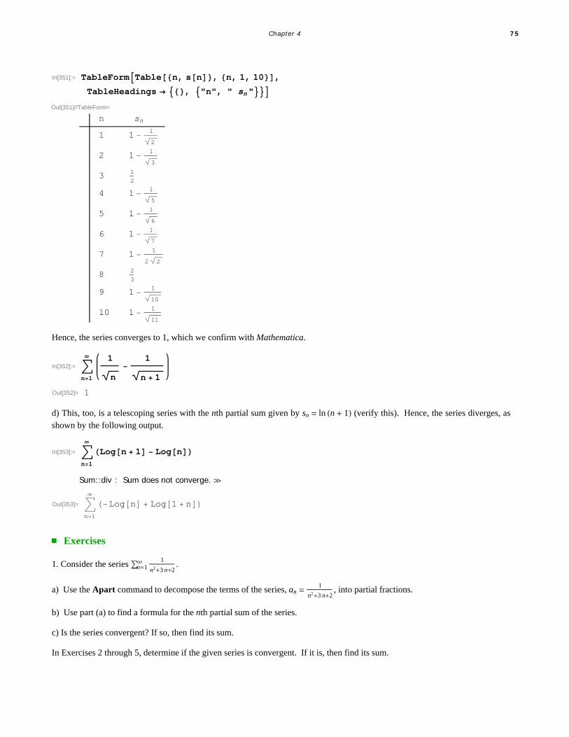
In[351]:= TableFormTablen, sn, n, 1, 10,
TableHeadings , "n", " sn "Out[351]//TableForm=
n sn
1 1 1
2
2 1 1
3
3 12
4 1 1
5
5 1 1
6
6 1 1
7
7 1 1
2 2
8 23
9 1 1
10
10 1 1
11
Hence, the series converges to 1, which we confirm with Mathematica.
In[352]:= n1
1
n
1
n 1
Out[352]= 1
d) This, too, is a telescoping series with the nth partial sum given by sn = ln n + 1 (verify this). Hence, the series diverges, asshown by the following output.
In[353]:= n1
Logn 1 Logn
Sum::div : Sum does not converge. à
Out[353]= n1
Logn Log1 n
ü Exercises
1. Consider the series n=1¶ 1
n2+3 n+2.
a) Use the Apart command to decompose the terms of the series, an =1
n2+3 n+2, into partial fractions.
b) Use part (a) to find a formula for the nth partial sum of the series.
c) Is the series convergent? If so, then find its sum.
In Exercises 2 through 5, determine if the given series is convergent. If it is, then find its sum.
Chapter 4 75
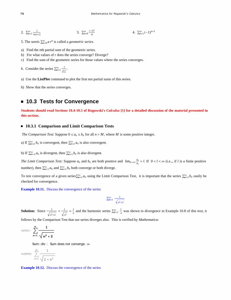
2. n=1¶ 1
nn+1 3. n=0¶ -1n
n!4. n=1
¶ -1n+1
5. The sereis n=0¶ a rn is called a geometric series.
a) Find the nth partial sum of the geometric series.b) For what values of r does the series converge? Diverge?c) Find the sum of the geometric series for those values where the series converges.
6. Consider the series n=1¶ 1
n3
.
a) Use the ListPlot command to plot the first ten partial sums of this series.
b) Show that the series converges.
ü 10.3 Tests for Convergence
Students should read Sections 10.4-10.5 of Rogawski's Calculus [1] for a detailed discussion of the material presented inthis section.
ü 10.3.1 Comparison and Limit Comparison Tests
The Comparison Test: Suppose 0 § an § bn for all n >M , where M is some positive integer.
a) If nã1¶ bn is convergent, then n=1
¶ an is also convergent.
b) If nã1¶ an is divergent, then n=1
¶ bn is also divergent.
The Limit Comparison Test: Suppose an and bn are both positive and limnضan
bn= l. If 0 < l <¶ (i.e.,, if l is a finite positive
number), then n=1¶ an and n=1
¶ bn both converge or both diverge.
To test convergence of a given seriesn=1¶ an using the Limit Comparison Test, it is important that the series n=1
¶ bn easily be
checked for convergence.
Example 10.11. Discuss the convergence of the series
n=1¶ 1
n2+2
Solution: Since 1
n2+2
< 1
n2
= 1
n and the harmonic series n=1
¶ 1
n was shown to divergence in Example 10.8 of this text, it
follows by the Comparison Test that our series diverges also. This is verified by Mathematica:
In[354]:= n1
1
n2 2
Sum::div : Sum does not converge. à
Out[354]= n1
1
2 n2
Example 10.12. Discuss the convergence of the series
76 Mathematica for Rogawski's Calculus

n=1¶ 3 n3+40 n2+4
n5+200 n4+1
Solution: To find another series to compare ours with, we consider one with terms bn =3
n2. This comes from considering lower
powers of n in both the numerator and denominator of an.
In[355]:= Cleara, b, n
an_ :3 n3 40 n2 4
n5 200 n4 1
bn_ :3
n2
In[358]:= Limit anbn , n Infinity
Out[358]= 1
Since the series n=1¶ 3
n2 is convergent (p-series) and limnض
an
bn= 1, we conclude from the Limit Comparison Test that our series
n=1¶ 3 n3+40 n2+4
n5+200 n4+1 is also convergent.
Example 10.13. Discuss the convergence of the series n=1¶ 1 - cos 1
n.
Solution: We note that limnض 1 - cos 1
n = 0. This is confirmed by Mathematica.
In[359]:= Limit1 Cos1 n, n Out[359]= 0
Thus, the necessary condition for convergence is satisfied. But this does not guarantee convergence. We will use the ListPlotcommand to plot the graph of the partial sums to see if the series converges.
In[360]:= Clearssn_ : Sum1 Cos1 k, k, 1, n
In[362]:= ListPlotTablen, sn, n, 1, 100, PlotRange 0, 1
Out[362]=
0 20 40 60 80 100
0.2
0.4
0.6
0.8
1.0
The graph above clearly indicates convergence. To see that this is indeed true, we compare it with a series that is known to
converge: n=1¶ 1
n2. To this end, let us define an and bn as follows.
Chapter 4 77
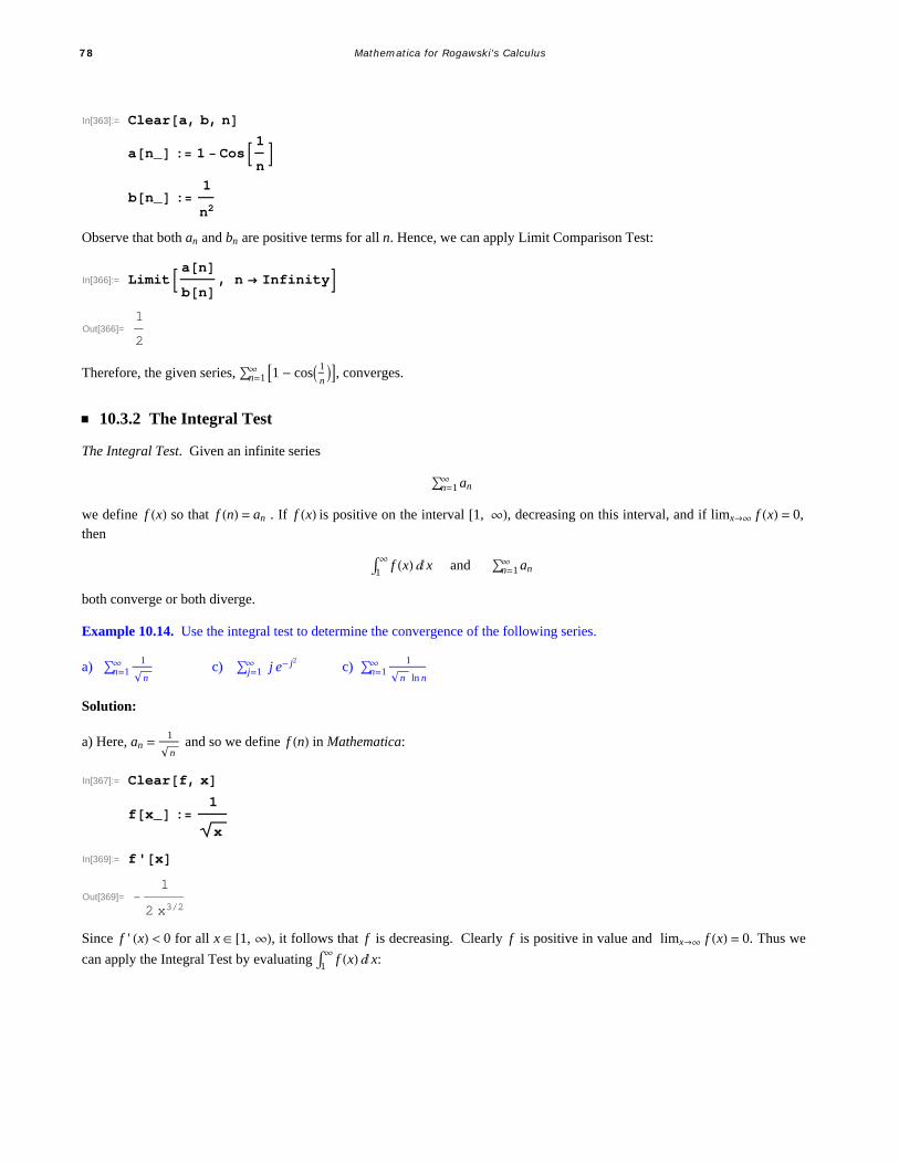
In[363]:= Cleara, b, nan_ : 1 Cos 1
n
bn_ :1
n2
Observe that both an and bn are positive terms for all n. Hence, we can apply Limit Comparison Test:
In[366]:= Limit anbn , n Infinity
Out[366]=1
2
Therefore, the given series, n=1¶ 1 - cos 1
n, converges.
ü 10.3.2 The Integral Test
The Integral Test. Given an infinite series
n=1¶ an
we define f x so that f n = an . If f x is positive on the interval 1, ¶, decreasing on this interval, and if limxض f x = 0,then
1¶
f x „ x and n=1¶ an
both converge or both diverge.
Example 10.14. Use the integral test to determine the convergence of the following series.
a) n=1¶ 1
nc) j=1
¶ j e- j2 c) n=1¶ 1
n ln n
Solution:
a) Here, an =1
n and so we define f n in Mathematica:
In[367]:= Clearf, xfx_ :
1
x
In[369]:= f'x
Out[369]= 1
2 x32
Since f ' x < 0 for all x œ 1, ¶, it follows that f is decreasing. Clearly f is positive in value and limxض f x = 0. Thus we
can apply the Integral Test by evaluating 1¶
f x „ x:
78 Mathematica for Rogawski's Calculus
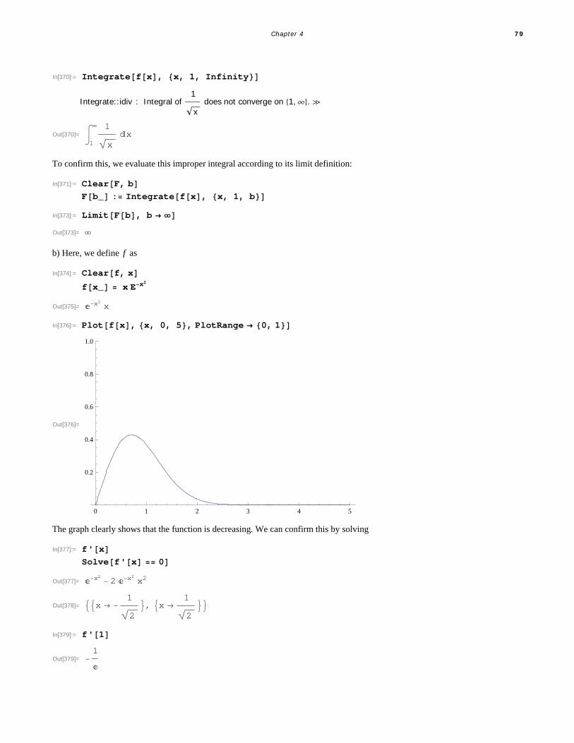
In[370]:= Integratefx, x, 1, Infinity
Integrate::idiv : Integral of 1
x does not converge on 1,¶. à
Out[370]= 1
1
xx
To confirm this, we evaluate this improper integral according to its limit definition:
In[371]:= ClearF, bFb_ : Integratefx, x, 1, b
In[373]:= LimitFb, b Out[373]=
b) Here, we define f as
In[374]:= Clearf, xfx_ x Ex2
Out[375]= x2x
In[376]:= Plotfx, x, 0, 5, PlotRange 0, 1
Out[376]=
0 1 2 3 4 5
0.2
0.4
0.6
0.8
1.0
The graph clearly shows that the function is decreasing. We can confirm this by solving
In[377]:= f'xSolvef'x 0
Out[377]= x2 2 x2
x2
Out[378]= x 1
2, x
1
2
In[379]:= f'1
Out[379]= 1
Chapter 4 79

In[380]:= N1 Sqrt2Out[380]= 0.707107
Thus, f has critical points at ±1
2º 0.707. Since f ' 1 < 0, we conclude that f is decreasing on 1, ¶.
The graph also shows that limxض f x = 0. Again, we can confirm this by evaluating
In[381]:= Limitfx, x InfinityOut[381]= 0
Hence, the Integral Test can be used to determine if the series is convergent. That the series j=1¶ j e- j2 is convergent follows
from the fact that
In[382]:= 1
fx x
Out[382]=1
2
Since the corresponding integral is convergent, it follows that the series j=1¶ j e- j2 is also convergent.
c) In this case, we define f as
In[383]:= Clearf, xfx_
1
x Logx
Out[384]=1
x LogxIn[385]:= Plotfx, x, 2, 100
Out[385]=
20 40 60 80 100
0.04
0.06
0.08
0.10
0.12
0.14
We leave it for the reader to check that f satisfies all the conditions of the Integral Test, which we now apply.
80 Mathematica for Rogawski's Calculus

In[386]:= 2
fx x
Integrate::idiv : Integral of 1
x Logx does not converge on 2,¶. à
Out[386]= 2
1
x Logxx
Since the preceding output states that the integral is divergent, we conclude that the corresponding series is divergent also.
Example 10.15. For what values of p does the series n=2¶ 1
nln np converge?
Solution: We apply the Integral Test. Toward this end, we define f x so that f n = 1
nln np and then verify that f x is positive
and decreasing on the interval a, ¶, and that limxض f x = 0:
In[387]:= Clearf, x, pfx_ :
1
x Logxp
In[389]:= Limitfx, x InfinityOut[389]= 0
To confirm this limit, we will plot graphs of f x for some values of p
In[390]:= PlotEvaluateTablefx, p, 4, 2, .5, x, 2, 100, PlotRange 0, 5
Out[390]=
0 20 40 60 80 100
1
2
3
4
5
In the plot above, observe that some of the graphs are initially increasing, but then begin to decrease at a certain point. Let usthen find the interval over which the function f x is decreasing for each p. To this end, we compute the derivative f ' x andsolve f ' x < 0 for x.
In[391]:= f'x
Out[391]= p Logx1p
x2
Logxp
x2
In[392]:= Simplify
Out[392]= Logx1p p Logx
x2
Chapter 4 81

In[393]:= Solvef'x 0, xOut[393]= x pSince (ln x-1-p > 0 for all x > 1, we see that f ' x < 0 if ln x > -p, or equivalently, x = ‰-p. Thus, f x is decreasing on 2, ¶where a is the maximum of 2 and ‰-p.
To apply the Integral Test, we integrate f over the interval 2, ¶. This is easier than integrating over the interval a, ¶, and
permissible since the integrals 2¶
f x „ x and a¶
f x „ x either converge or diverge together.
In[394]:= Integratefx, x, 2,
Out[394]= ConditionalExpressionLog21p
1 p, Rep 1
The preceding output shows that 2¶
f x „ x is convergent for p > 1. However, the case p § 1 remains unsolved. To evaluate the
integral in this situation, we define its anti-derivative Fb = 2b
f x „ x and find the limit of Fb as bØ ¶.
In[395]:= ClearF, bFb_ Integratefx, x, 2, b
Out[396]= ConditionalExpressionLog21p Logb1p
1 p, Reb 1 b Reals
Since b is a real number and b > 2 , the solution to our integral is the first one, that is, Fb = ln 21-p-ln b1-p
1-p, provided p ∫ 1. But
then for p < 1, we see that limbضFb =¶ since limbض lnb1-p =¶. For p > 1, we have limbضFb = ln 21-p
1-p, which we
already knew from the second previous Mathematica output. The following tables might be helpful to convince you about this.
In[397]:= TableLimitFb, b Infinity, p, 3, .9, .5Out[397]= , , , , , , , In[398]:= TableLimitFb, b Infinity, p, 1.1, 9, .5Out[398]= 10.3733, 2.0766, 1.3605, 1.12346, 1.02813, 0.997425, 1.0048, 1.03926,
1.09605, 1.1734, 1.27122, 1.39056, 1.53333, 1.70219, 1.90056, 2.13262For p = 1, we make this substitution inside the integral and evaluate it directly:
In[399]:= p 1;Integratefx, x, 2,
Integrate::idiv : Integral of 1
x Logx does not converge on 2,¶. à
Out[400]= 2
1
x Logx x
Therefore, the infinite series n=2¶ 1
nln np is convergent for p > 1 and divergent for p § 1.
NOTE: To see how slow the growth of this series is for the value of p = 1, we consider the following table of partial sums. Recallthat f n is the nth term of the series and hence the nth partial sum is given by
82 Mathematica for Rogawski's Calculus
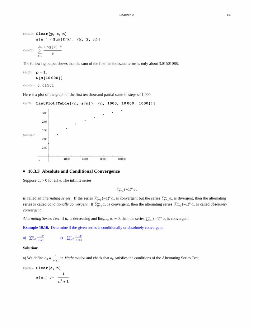
In[401]:= Clearp, s, nsn_ Sumfk, k, 2, n
Out[402]= k2
n Logkp
k
The following output shows that the sum of the first ten thousand terms is only about 3.01501088.
In[403]:= p 1;
Ns10 000Out[404]= 3.01501
Here is a plot of the graph of the first ten thousand partial sums in steps of 1,000.
In[405]:= ListPlotTablen, sn, n, 1000, 10 000, 1000
Out[405]=
4000 6000 8000 10 000
2.80
2.85
2.90
2.95
3.00
ü 10.3.3 Absolute and Conditional Convergence
Suppose an > 0 for all n. The infinite series
n=1¶ -1n an
is called an alternating series. If the series n=1¶ -1n an is convergent but the series n=1
¶ an is divergent, then the alternating
series is called conditionally convergent. If n=1¶ an is convergent, then the alternating series n=1
¶ -1n an is called absolutely
convergent.
Alternating Series Test: If an is decreasing and limnضan = 0, then the series n=1¶ -1n an is convergent.
Example 10.16. Determine if the given series is conditionally or absolutely convergent.
a) n=1¶ -1n
n2+1c) n=2
¶ -1n
n ln n
Solution:
a) We define an =1
n2+1 in Mathematica and check that an satisfies the conditions of the Alternating Series Test.
In[406]:= Cleara, nan_ :
1
n2 1
Chapter 4 83

In[408]:= Limitan, n Out[408]= 0
In[409]:= fx_ ax;
f'x
Out[410]= 2 x
1 x22
Thus, an is decreasing since f ' x > 0, where f n = an. Moreover, an converges to 0. Hence, the series n=1¶ -1n
n2+1 is convergent
by the Alternating Series Test.
To check absolute convergence, we use the Limit Comparison Test with bn =1
n2.
In[411]:= Limit an1 n2
, n Infinity
Out[411]= 1
Since the series n=1¶ 1
n2 is convergent and the previous output shows limnض
an
bn= 1, we conclude that the series
n=1¶ an =n=1
¶ 1
n2+1 is also convergent. Therefore, the alternating series n=1
¶ -1n
n2+1 is absolutely convergent.
b) We procced as in part a).
In[412]:= Cleara, nan_ :
1
n LognIn[414]:= Limitan, n Out[414]= 0
In[415]:= fx_ ax;
f'x
Out[416]= 1
x2 Logx2
1
x2 Logx
For the same reasons we conclude that an is decreasing and converges to 0. Hence, the series n=2¶ -1n
n ln n is convergent by the
Alternating Series Test.
To check absolute convergence, we apply the Intgeral Test to f x:In[417]:= Clearm
Limit2
m
fx x, m InfinityOut[418]=
From this, we conclude that the series is conditionally convergent.
Example 10.17. Show that the series
84 Mathematica for Rogawski's Calculus

n=1¶ -1n
n2+1
is conditionally convergent. Find a value of n for which the partial sum sn approximates the series by an error less than 10-5.Also, find the corresponding value for sn.
Solution: We leave it for the reader to check that the series converges conditionally as in the preceding example. For the secondpart of the problem, we proceed by first defining the partial sums of the series.
In[419]:= Clears, a, nan_ :
1
n2 1
sn_ : Sum1k ak, k, 1, nIf S denotes the sum of the alternating series, it can be shown that S - sn < an+1 (refer to your calculus text for a proof of thisfact). The following table of values gives some numerical evidence of this fact:
n1
1n
1 n2
In[422]:= TableNAbsn1
1n
n2 1
sm, Nam, m, 1, 10
Out[422]= 0.266189, 0.707107, 0.181024, 0.447214,0.135203, 0.316228, 0.107332, 0.242536, 0.088784, 0.196116,0.075615, 0.164399, 0.0658064, 0.141421, 0.0582284, 0.124035,0.0522031, 0.110432, 0.0473006, 0.0995037
In[423]:= ClearS, nS
n1
1n
n2 1
Out[424]= n1
1n
1 n2
The table below gives the values of an for large values of n.
In[425]:= TableNa10n , n, 1, 10 Out[425]= 0.0995037, 0.0099995, 0.001, 0.0001,
0.00001, 1. 106, 1. 107, 1. 108, 1. 109, 1. 1010
Thus, n = 106 is a possible value. But solving an = 10-5 can give us a more accurate value.
In[426]:= NSolveax 105, xOut[426]= x 100 000., x 100 000.Thus, if n = 100 001, we have S - sn < 10-5. We confirm this with Mathematica:
Chapter 4 85

In[427]:= NS s100 001Out[427]= 4.99993 106
Can you find a smaller value of n for which S - sn < 10-5?
ü 10.3.4 Ratio Test
The Ratio Test: Suppose an > 0 and let
r = limnضan+1
an.
a) If r < 1, the series n=1¶ an converges.
b) If r > 1, the series n=1¶ an diverges.
c) If r = 1, no conclusion can be drawn about the convergence of the series n=1¶ an. In other words, if r = 1, then we must use
another test to determine the convergence.
Example 10.18. Use the Ratio Test to determine the convergence of the following series.
a) n=1¶ nn
n!c) j=2
¶ 1
j ln j3c) n=1
¶ 3 n3+40 n2+4
n5+200 n4+1
Solution: For each series, we define an to be its nth term and evaluate limnضan+1
an.
a)
In[428]:= Cleara, nan_ :
nn
n
In[430]:= Limitan 1 an, n Out[430]=
Since ‰ > 1, the series n=1¶ nn
n! converges by the Ratio Test.
b)
In[431]:= Cleara, jaj_ :
1
j Logj3
Limitaj 1 aj, j Out[433]= 1
This output means that we must use a different test. However, this is an instance of Example 11.12 in this text with p = 3. Hence,the series converges by the Integral Test.
c)
In[434]:= Cleara, n
an_ :3 n3 40 n2 1
n5 200 n4 1
86 Mathematica for Rogawski's Calculus

In[436]:= Limitan 1 an, n Out[436]= 1
Again, this output means we are forced to use a different test. Therefore, we shall use the Limit Comparison Test instead. To this
end, we define bn =3
n2:
In[437]:= Clearb, nbn_ :
3
n2
In[439]:= Limit anbn , n Infinity
Out[439]= 1
Since the series n=1¶ 1
n2 is convergent, we conclude that the series n=1
¶ 3 n3+40 n2+4
n5+200 n4+1 is also convergent.
ü 10.3.5 Root Test
The Root Test: Suppose an > 0 and let
r = limnض an1n.
a) If r < 1, the series n=1¶ anconverges.
b) If r > 1, the series n=1¶ an diverges.
c) If r = 1, no conclusion can be drawn about the convergence of the series n=1¶ an. In other words, if r = 1, then we must use
another test to determine the convergence.
Example 10.19. Use the Root Test to determine the convergence of the following series:
a) n=1¶ n
2 n+1n
b) n=1¶ 1
n 3n+n2c) n=1
¶ 3 n+1
n2+n+1
Solution: For each series we define an to be its nth term and evaluate limnض an1n.
a)
In[440]:= Cleara, nan_ :
n
2 n 1
n
In[442]:= Limitan1n, n
Out[442]=1
2
Thus, the series n=1¶ n
2 n+1n
converges by Root Test.
b)
In[443]:= Cleara, nan_ :
1
n 3n n2
Chapter 4 87
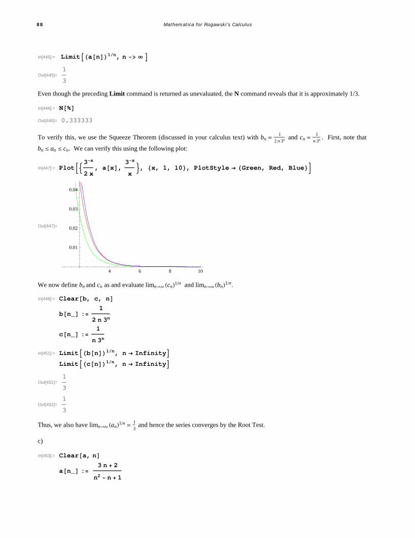
In[445]:= Limitan1n, n
Out[445]=1
3
Even though the preceding Limit command is returned as unevaluated, the N command reveals that it is approximately 1/3.
In[446]:= NOut[446]= 0.333333
To verify this, we use the Squeeze Theorem (discussed in your calculus text) with bn =1
2 n 3n and cn =1
n 3n . First, note that
bn § an § cn. We can verify this using the following plot:
In[447]:= Plot 3x
2 x, ax,
3x
x, x, 1, 10, PlotStyle Green, Red, Blue
Out[447]=
4 6 8 10
0.01
0.02
0.03
0.04
We now define bn and cn as and evaluate limnض cn1n and limnض bn1n.
In[448]:= Clearb, c, nbn_ :
1
2 n 3n
cn_ :1
n 3n
In[451]:= Limitbn1n, n InfinityLimitcn1n, n Infinity
Out[451]=1
3
Out[452]=1
3
Thus, we also have limnض an1n = 1
3 and hence the series converges by the Root Test.
c)
In[453]:= Cleara, nan_ :
3 n 2
n2 n 1
88 Mathematica for Rogawski's Calculus
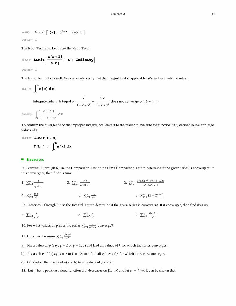
In[455]:= Limit an1n, n Out[455]= 1
The Root Test fails. Let us try the Ratio Test:
In[456]:= Limit an 1an , n Infinity
Out[456]= 1
The Ratio Test fails as well. We can easily verify that the Integral Test is applicable. We will evaluate the integral
In[457]:= 1
ax x
Integrate::idiv : Integral of 2
1 - x + x2+
3 x
1 - x + x2 does not converge on 1,¶. à
Out[457]= 1
2 3 x
1 x x2x
To confirm the divergence of the improper integral, we leave it to the reader to evalaute the function Fx defined below for largevalues of x.
In[458]:= ClearF, bFb_ :
1
b
ax x
ü Exercises
In Exercises 1 through 6, use the Comparison Test or the Limit Comparison Test to determine if the given series is convergent. Ifit is convergent, then find its sum.
1. n=1¶ n
n3+1
2. n=2¶ ln n
n2+3 ln n3. n=1
¶ n4+200 n2+1000 n+2222
n6+5 n4+n+1
4. n=1¶ ln n
n2 5. n=2
¶ 1
nln n6. n=1
¶ 1 - 2-1n
In Exercises 7 through 9, use the Integral Test to determine if the given series is convergent. If it converges, then find its sum.
7. n=1¶ n
n2+18. n=2
¶ n
2n 9. n=1¶ ln n3
n2
10. For what values of p does the series n=1¶ 1
np ln n converge?
11. Consider the series n=2¶ ln nk
np .
a) Fix a value of p (say, p = 2 or p = 1 2) and find all values of k for which the series converges.
b) Fix a value of k (say, k = 2 or k = -2) and find all values of p for which the series converges.
c) Generalize the results of a) and b) to all values of p and k.
12. Let f be a positive valued function that decreases on 1, ¶ and let an = f n. It can be shown that
Chapter 4 89

1
¶f x „ x §n=1
¶ an § a1 + 1
¶f x „ x .
a) Use f x = 1
x1.1 to verify this.
b) Approximate n=1¶ 1
n1.1 using its nth partial sums with n = 10, 100, 1000, 10 000.
In Exercises 13 through 16, determine if each of the infinite series is absolutely convergent, conditionally convergent, or diver-
gent. Justify your conclusions!
13. n=1¶ -1n n2-1
n2+114. n=1
¶ 20 n2-n-1
n3+n2+3315. n=1
¶ -2n
n!16. n=1
¶ -1n+1 n + 1 - n ]
17. Discovery Exercise:
a) Determine the convergence or divergence of n=2¶ 1
n ln ln ln n0.5, n=2
¶ 1
n ln ln ln n , and n=2¶ 1
n ln ln ln n2.
b) Generalize your work in part a) by determining for which real numbers p the seriesn=2¶ 1
n ln ln ln np converges.
In Exercises 18 through 25, determine the convergence or divergence of the given infinite series using any of the convergencetests discussed in this section.
18. n=1¶ 3 n+1
4 n+519. n=1
¶ n
2 n2+1 20. n=1
¶ n+3
4 n3+5 21. n=1
¶ n 2
3n
22. n=1¶ n 3
2n
23. n=1¶ nn
n!24. n=1
¶ n!2
3 n! 25. n=0¶ -1n 1 + 1
nn
26. The Ratio Test proved to be inconclusive for some of the series in the previous exercise. Can you conjecture for what type ofseries the Ratio Test will fail in general? Use other tests to rework the problems in the first exercise where the Ratio Test failed.
27. Of the following four conditions, one guarantees that a series will diverge, two conditions guarantee that a series will con-verge, and one has no guarantee (the series can either converge or diverge). Identify each one and explain your reasoning.
limnضan+1
an= 0
limnضan+1
an= 1
2
limnضan+1
an= 1
limnضan+1
an= 2
28. Identify the two series that are the same:
a) n=1¶ n 3
4n
b) n=0¶ n + 1 3
4n
c) n=1¶ n 3
4n-1
In Exercises 29 through 32, determine the convergence or divergence of the series:
29. n=1¶ 2 n
n
+1) n 30, n=0¶ e-n 31. n=1
¶ -2 n
3 n+13 n
32. n=1¶ n
2 n+1) n
33. Construct two examples of infinite series, the first convergent and the second divergent, for which the Root Test generatesinconclusive information.
34. Use the Root Test to test for convergence or divergence of the series:
90 Mathematica for Rogawski's Calculus

a) 1
ln 33+ 1
ln 44+ 1
ln 55+ 1
ln 66+ ...
b) 1+ 2
3+ 3
32+ 4
33+ 5
34+
6
35+...
Hint: Write a formula for the general nth term in each case.
ü 10.4 Power Series
Students should read Sections 10.6-10.7 of Rogawski's Calculus [1] for a detailed discussion of the material presented inthis section.
ü 10.4.1 Taylor Polynomials
The Taylor polynomial of a given function f at a point x = a is given by
Tnx = f a + f ' a x - a + f '' a2!
x - a2 +f ''' a
3!x - a3 + ....+
f nan!
x - an.
The Mathematica Series[f,{x, a, n}] generates the nth Taylor polynomial Tnx plus a term of the form Oxn+1. To obtain the
Taylor polynomial without this term, we use the command Normal[Series[f,{x, a, n}]].
The nth remainder Rnx of f x at x = a is defined by
Rnx = f x - Tnx.Taylor's Theorem states that
Rnx = 1
n! a
xf n+1u x - un „u.
Here is a way to define the Taylor polynomial of f at x = a by defining Tnx and the nth remainder Rnx (using Taylor's Theo-
rem for Rn) without referring to Mathematica's built-in command Series.
In[460]:= Cleara, x, f, T, RTx_, a_, n_ :
k0
n Dfx, x, k . x a
kx ak
Rx_, a_, n_ :1
n
a
x
Dfu, u, n 1 x un u
Example 10.20. Let f x = ex. Find its 5th Taylor polynomial at x = 0.
Solution: We use the Series command to obtain the answer:
In[463]:= NormalSeriesEx, x, 0, 5
Out[463]= 1 x x2
2
x3
6
x4
24
x5
120
Using the polynomial Tx, a, n, we defined above we get
Chapter 4 91
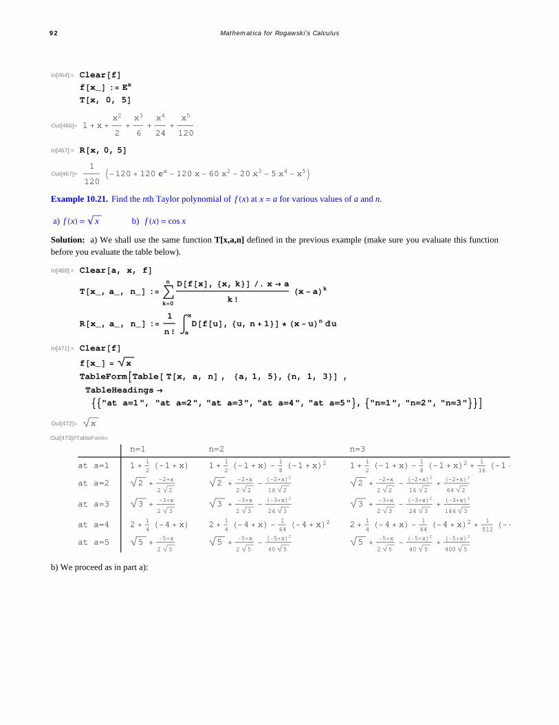
In[464]:= Clearffx_ : Ex
Tx, 0, 5
Out[466]= 1 x x2
2
x3
6
x4
24
x5
120
In[467]:= Rx, 0, 5
Out[467]=1
120120 120 x 120 x 60 x2 20 x3 5 x4 x5
Example 10.21. Find the nth Taylor polynomial of f x at x = a for various values of a and n.
a) f x = x b) f x = cos x
Solution: a) We shall use the same function T[x,a,n] defined in the previous example (make sure you evaluate this functionbefore you evaluate the table below).
In[468]:= Cleara, x, fTx_, a_, n_ :
k0
n Dfx, x, k . x a
kx ak
Rx_, a_, n_ :1
n
a
x
Dfu, u, n 1 x un u
In[471]:= Clearffx_ x
TableFormTable Tx, a, n , a, 1, 5, n, 1, 3 ,
TableHeadings
"at a=1", "at a=2", "at a=3", "at a=4", "at a=5", "n=1", "n=2", "n=3"Out[472]= x
Out[473]//TableForm=
n=1 n=2 n=3
at a=1 1 121 x 1 1
21 x 1
81 x2 1 1
21 x 1
81 x2 1
161
at a=2 2 2x
2 22 2x
2 2 2x2
16 22 2x
2 2 2x2
16 2 2x3
64 2
at a=3 3 3x
2 33 3x
2 3 3x2
24 33 3x
2 3 3x2
24 3 3x3
144 3
at a=4 2 144 x 2 1
44 x 1
644 x2 2 1
44 x 1
644 x2 1
5124
at a=5 5 5x
2 55 5x
2 5 5x2
40 55 5x
2 5 5x2
40 5 5x3
400 5
b) We proceed as in part a):
92 Mathematica for Rogawski's Calculus

In[474]:= Clearffx_ CosxTableFormTable Tx, a, n , a, 0, 2 Pi, Pi 2, n, 1, 4 ,
TableHeadings "at a=0", "at a=/2", "at a=", "at a=3/2", "at a=2",
"n=1", "n=2", "n=3", "n=4"Out[475]= CosxOut[476]//TableForm=
n=1 n=2 n=3 n=4
at a=0 1 1 x2
21 x2
21 x2
2 x4
24
at a=/2
2 x
2 x
2 x 1
6
2 x3
2 x 1
6
2 x3
at a= 1 1 12 x2 1 1
2 x2 1 1
2 x2 1
24
at a=3/2 3
2 x 3
2 x 3
2 x 1
6 3
2 x3
3
2 x 1
6 3
2 x3
at a=2 1 1 122 x2 1 1
22 x2 1 1
22 x2 1
242
Example 10.22. Let f x = 1
2+3 x2.
a) Find the Taylor polynomials Tnx of f at x = 0 for n = 1, 2, ..., 6.b) Draw the graphs of the function f and its Taylor polynomials found in part a).c) Over which interval does the nth Taylor polynomial gives a close approximation to f x if n = 4, n =10, and n = 20?
Solution:
a) Here are the Taylor polynomials up to order n = 6.
In[477]:= Clearffx_
1
2 3 x2
TableFormTable n, Tx, 0, n , n, 1, 6 ,
TableHeadings , "n", "Tn at a=0"
Out[478]=1
2 3 x2
Out[479]//TableForm=
n Tn at a=0
1 12
2 12 3 x2
4
3 12 3 x2
4
4 12 3 x2
4 9 x4
8
5 12 3 x2
4 9 x4
8
6 12 3 x2
4 9 x4
8 27 x6
16
b) We first use the Plot command to plot the graphs of f and its Taylor polynomial at x = 0 for the desired values of n. We then
use the Show command to plot both graphs on the same axes.
Chapter 4 93

In[480]:= Clearplot1, plot2plot1 Plotfx, x, 3, 3, PlotStyle Red;plot2 PlotEvaluateTableTx, 0, n, n, 1, 6, x, 3, 3 ;Showplot1, plot2
Out[483]=
-3 -2 -1 1 2 3
0.1
0.2
0.3
0.4
0.5
c) We use the same commands as in part b) except that we do not use the Table command. The first one is for the case n = 4.
In[484]:= Clearplot1, plot2plot1 Plotfx, x, 3, 3, PlotStyle Red;plot2 PlotEvaluateTx, 0, 4, x, 3, 3 ;
Showplot1, plot2
Out[487]=
-3 -2 -1 1 2 3
0.1
0.2
0.3
0.4
0.5
It seems that the two graphs are close to each other if x is in the interval -0.5, 0.5. To see this close up, we recommend thatyou change the range of values for x in both plots (plot1 and plot2) to the interval -1, 1. We can confirm this by plotting the 4thremainder of f x at x = 0.
94 Mathematica for Rogawski's Calculus

In[488]:= PlotEvaluateRx, 0, 4, x, 1, 1, PlotRange 1, 1
Out[488]=-1.0 -0.5 0.5 1.0
-1.0
-0.5
0.5
1.0
We repeat the above with n = 10.
In[489]:= Clearplot1, plot2plot1 Plotfx, x, 3, 3, PlotStyle Red;plot2 PlotEvaluateTx, 0, 100, x, 3, 3 ;
Showplot1, plot2
Out[492]=
-3 -2 -1 1 2 3
0.1
0.2
0.3
0.4
0.5
The graph above clearly indicates the 10th Taylor polynomial gives a close approximation for f in the interval -.6, .6. Again,plotting Rn will confirm this.
Chapter 4 95

In[493]:= PlotEvaluateRx, 0, 10, x, 1, 1, PlotRange 1, 1
Out[493]=-1.0 -0.5 0.5 1.0
-1.0
-0.5
0.5
1.0
If we continue in this manner, we see that the Taylor polynomial Pn for large values of n gives a better approximation of f in theinterval -1, 1. In fact, for n = 20, we see that Rnx is almost zero in the interval -0.7, 0.7, which is an improvement over theprevious interval -0.6, 0.6 obtained for n = 10.
In[494]:= PlotEvaluateRx, 0, 20, x, 1, 1, PlotRange 1, 1
Out[494]=-1.0 -0.5 0.5 1.0
-1.0
-0.5
0.5
1.0
ü 10.4.2 Convergence of Power Series
A series of the form
n=0¶ anx - x0n = a0 + a1x - x0 + a2x - x02 + a3x - x03 + ....
is called a power series.
The set of all x for which the series converges is called the interval of convergence.
If the series converges for x = x0 only, we say is radius of interval is R = 0. In this case, its interval of convergence is x0.If the series converges for all real numbers x, we say its radius of convergence is R =¶. In this case, its interval of convergenceis -¶, ¶.
96 Mathematica for Rogawski's Calculus

If the series converges for some x ∫ x0 and diverges for some y, then it can be shown that there exists R > 0 such that the powerseries converges for all x for which x - x0 < R and diverges for all x for which x - x0 > R. The convergence at x = x0 - Rand x = x0 + R needs to be checked.
When the radius of convergence R is a positive real number, there are four possiblities for the interval of convergence:
x0 - R, x0 + R or x0 - R, x0 + R or x0 - R, x0 + R or x0 - R, x0 + R depending on the convergence at the end points of the intervals.
The radius of convergence R of the power series n=0¶ anx - x0n can be found by using the Ratio or Root Test. Let
r = limnضan+1
an or r = limnض an
n
a) If r = 0, then R =¶. b) If r =¶, then R = 0 .
c) If 0 < r <¶, then R = 1
r.
Example 10.23. Find the radius and interval of convergence for the given power series.
a) n=0¶ n
2 n+1xn b) n=1
¶ x-3n
n 3n c) n=0¶ x+2n
n2+n+1
d) n=0¶ nn xn e) n=0
¶ 1
n!x - 1n
Solution:
a) Let us define smx to be the mth partial sum of the series and plot the graph of some of these partial sums. We will plot every100th partial sum up to 10,000 terms.
In[495]:= Clears, n, msx_, m_ :
n0
m n
2 n 1xn
In[497]:= PlotEvaluateTablesx, m, m, 1, 1000, 100, x, 2, 2
Out[497]=
-2 -1 1 2
-2μ1026
2μ1026
4μ1026
This clearly indicates that the partial sums diverge outside -1, 1. Here is the plot over the interval -1, 1.
Chapter 4 97

In[498]:= PlotEvaluateTablesx, m, m, 1, 1000, 100, x, 1, 1
Out[498]=
-1.0 -0.5 0.5 1.0
0.5
1.0
1.5
We now use calculus. Here, note that an =n
2 n+1 and x0 = 0. We first define an in Mathematica and find the radius of conver-
gence. We recall a (absolute value of a) is entered as Abs[a].
In[499]:= Cleara, n, ran_ :
n
2 n 1
In[501]:= r LimitAbsan 1an , n Infinity
Out[501]= 1
Thus, the radius of convergence is R = 1
r= 1
1= 1. The power series convrges on -1, 1. To check convergence at the endpoints
x = -1 and x = 1, we note that the power series becomes n=0¶ n
2 n+1-1nand n=0
¶ n
2 n+11n, both of which are divergent, since
their nth terms do not converge to 0. Here, Mathematica confirms the divergence at the endpoints.
In[502]:= n0
n
2 n 11n
Sum::div : Sum does not converge. à
Out[502]= n0
1n n
1 2 n
In[503]:= n0
n
2 n 11n
Sum::div : Sum does not converge. à
Out[503]= n0
n
1 2 n
Therefore, the interval of convergence is -1, 1.
b) n=1¶ x-3n
n 3n
98 Mathematica for Rogawski's Calculus

In[504]:= Cleara, r, nan_ :
1
n 3n
In[506]:= r Limit an 1an , n Infinity
Out[506]=1
3
Thus the radius of convergence is R = 1
r= 1
13 = 3.
Since x0 = 3, the power series converges on x0 - R, x0 + R = 3 - 3, 3 + 3 = 0, 6. We need to check the endpoints x = 0 andx = 6. We substitute these in the power series and evaluate
In[507]:= n1
x 3n
n 3n. x 0, 6
Out[507]= Log2, Thus, the interval of convergence is 0, 6.
c) n=1¶ x+2n
n2+n+1
In[508]:= Cleara, r, nan_ :
1
n2 n 1
In[510]:= r LimitAbs an 1an , n
Out[510]= 1
Hence, the radius of convergence is R = 1
1= 1. Since x0 = -2, we see that the power series converges at least on the open interval
-2 - 1, -2 + 1 = -3, -1. To determine the actual interval of convergence we need to check the endpoints. As in part c), weevaluate
In[511]:= n0
x 2n
n2 n 1. x 3, 1
Out[511]= HypergeometricPFQ1, 113, 123, 3
2 3
2,
3
2 3
2, 1,
HypergeometricPFQ1, 113, 123, 3
2 3
2,
3
2 3
2, 1
In[512]:= NOut[512]= 0.76131 4.70246 1016 , 1.79815 4.96787 1016 Since this is not clear, we examine the series by plugging in by hand x = -3 and x = -1. When x = -3 the series becomes
n=1¶ -3+2n
n2+n+1= n=1
¶ -1n
n2+n+1, which is an alternating series. We leave it to the reader to verify that the Alternating Series Test
applies in this case. Thus, we have a convergent series.
Chapter 4 99

Next, we substitute x = -1 to obtain the series n=1¶ -1+2n
n2+n+1= n=1
¶ 1
n2+n+1 to which we apply the Integral Test (verify that the
conditions of the Integral Test are satisfied):
In[513]:= Integrate 1
x2 x 1, x, 0, Infinity
Out[513]=2
3 3
Thus, the series converges in this case as well. Therefore, the interval of convergence for the power series is -3, -1. d) n=0
¶ nn xn
In[514]:= Cleara, r, nan_ : nn
In[516]:= r LimitAbs an 1an , n
Out[516]=
Thus, the radius of convergence is R = 0 and the series converges for x = 0 only.
e) n=0¶ 1
n!x - 1n
In[517]:= Cleara, r, nan_ :
1
n
In[519]:= r LimitAbs an 1an , n
Out[519]= 0
Thus, the radius of convergence is R =¶ and the series converges for all real x. Hence, the interval of convergence is -¶, ¶.
ü 10.4.3 Taylor Series
The Taylor series for f x at x = a is given by the power series
n=0¶ f na
n!x - an = f a + f ' a x - a + f '' a
2x - a2 +
f ''' a6
x - a3 + .....
The Mathematica command Series[f,{x, a, n}] generates the power series of f at x = a to the order x - an. It is not possible towrite all the terms explicitly since there are infinitely many.
Example 10.24. Let f x = 1+x
1+x2.
a) Find the first ten terms of the Taylor series of f at x = 0.b) Estimate the radius and interval of convergence of the Taylor series of f at x = 0.
Solution:
a) We use the Series command to obtain the Taylor series as follows:
100 Mathematica for Rogawski's Calculus

In[520]:= Clearf, xfx_ :
1 x
2 x
In[522]:= Seriesfx, x, 0, 10
Out[522]=1
2
3 x
4
3 x2
8
3 x3
16
3 x4
32
3 x5
64
3 x6
128
3 x7
256
3 x8
512
3 x9
1024
3 x10
2048 Ox11
This output gives the Taylor series to order n = 10.
b) To first gain intuition for the radius of convergence of the Taylor series, we define the nth Taylor polynomial of f x as a
function of n (note our use of the Normal command to truncate the remainder term from the Taylor series).
In[523]:= ClearT, x, nTx_, n_ : NormalSeriesfx, x, 0, n
Here is a list of the first 20 of these polynomials.
In[525]:= TableTx, n, n, 0, 10
Out[525]= 1
2,
1
2
3 x
4,
1
2
3 x
4
3 x2
8,
1
2
3 x
4
3 x2
8
3 x3
16,
1
2
3 x
4
3 x2
8
3 x3
16
3 x4
32,
1
2
3 x
4
3 x2
8
3 x3
16
3 x4
32
3 x5
64,
1
2
3 x
4
3 x2
8
3 x3
16
3 x4
32
3 x5
64
3 x6
128,
1
2
3 x
4
3 x2
8
3 x3
16
3 x4
32
3 x5
64
3 x6
128
3 x7
256,
1
2
3 x
4
3 x2
8
3 x3
16
3 x4
32
3 x5
64
3 x6
128
3 x7
256
3 x8
512,
1
2
3 x
4
3 x2
8
3 x3
16
3 x4
32
3 x5
64
3 x6
128
3 x7
256
3 x8
512
3 x9
1024,
1
2
3 x
4
3 x2
8
3 x3
16
3 x4
32
3 x5
64
3 x6
128
3 x7
256
3 x8
512
3 x9
1024
3 x10
2048
Observe that each polynomial appears twice, that is, T2 n = T2 n+1, since f is an even function. Next, we plot the graphs of someof these polynomials:
Chapter 4 101
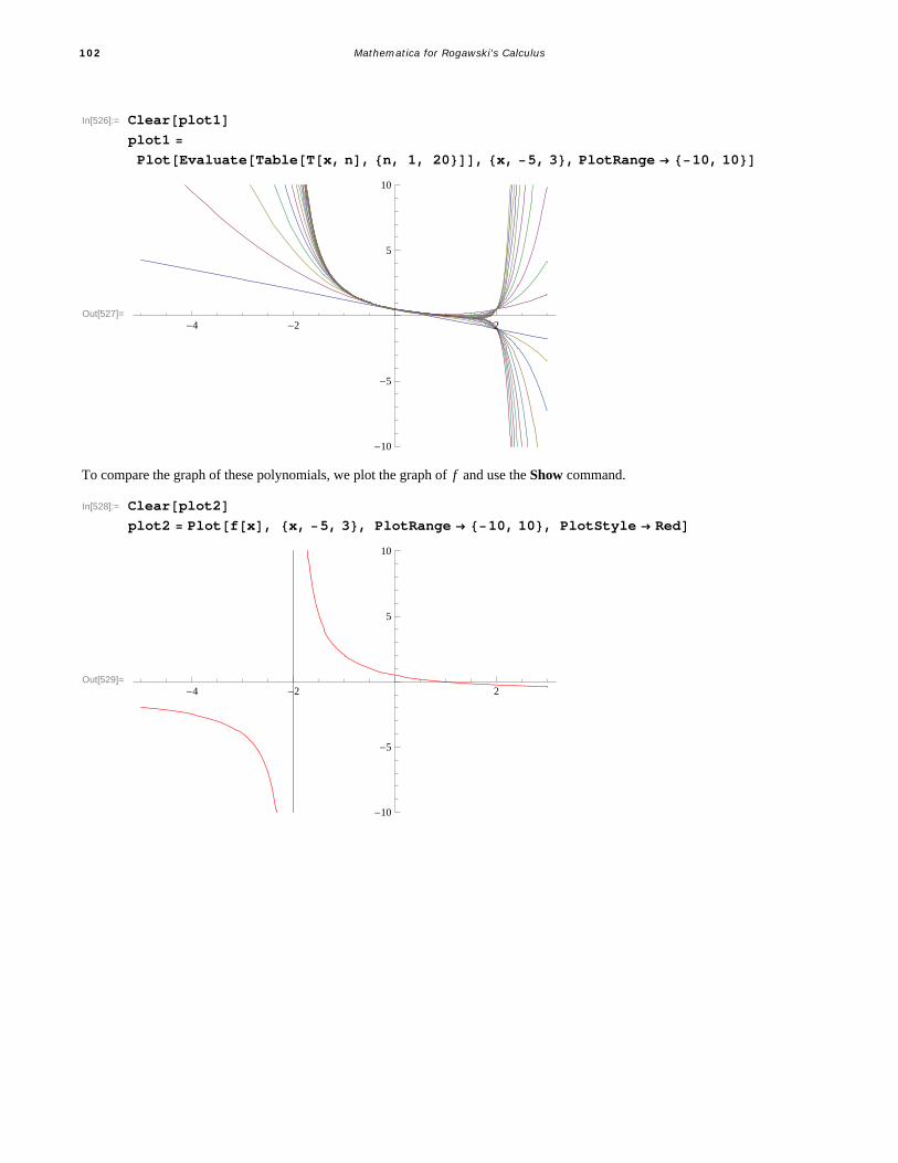
In[526]:= Clearplot1plot1
PlotEvaluateTableTx, n, n, 1, 20, x, 5, 3, PlotRange 10, 10
Out[527]=-4 -2 2
-10
-5
5
10
To compare the graph of these polynomials, we plot the graph of f and use the Show command.
In[528]:= Clearplot2plot2 Plotfx, x, 5, 3, PlotRange 10, 10, PlotStyle Red
Out[529]=-4 -2 2
-10
-5
5
10
102 Mathematica for Rogawski's Calculus
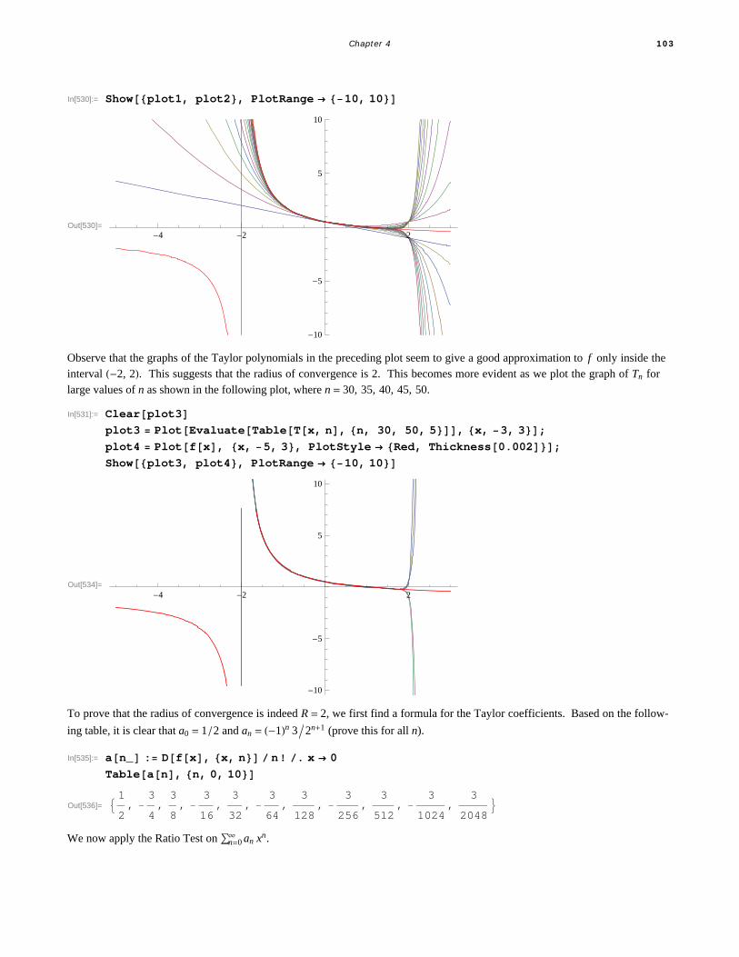
In[530]:= Showplot1, plot2, PlotRange 10, 10
Out[530]=-4 -2 2
-10
-5
5
10
Observe that the graphs of the Taylor polynomials in the preceding plot seem to give a good approximation to f only inside theinterval -2, 2. This suggests that the radius of convergence is 2. This becomes more evident as we plot the graph of Tn forlarge values of n as shown in the following plot, where n = 30, 35, 40, 45, 50.
In[531]:= Clearplot3plot3 PlotEvaluateTableTx, n, n, 30, 50, 5, x, 3, 3;
plot4 Plotfx, x, 5, 3, PlotStyle Red, Thickness0.002;Showplot3, plot4, PlotRange 10, 10
Out[534]=-4 -2 2
-10
-5
5
10
To prove that the radius of convergence is indeed R = 2, we first find a formula for the Taylor coefficients. Based on the follow-
ing table, it is clear that a0 = 1 2 and an = -1n 32n+1 (prove this for all n).
In[535]:= an_ : Dfx, x, n n . x 0
Tablean, n, 0, 10
Out[536]= 1
2,
3
4,
3
8,
3
16,
3
32,
3
64,
3
128,
3
256,
3
512,
3
1024,
3
2048
We now apply the Ratio Test on n=0¶ an xn.
Chapter 4 103

In[537]:= Clearaan_ 1^n 3 2^n 1r LimitAbs an 1
an , n
Out[538]= 3 1n 21n
Out[539]=1
2
Hence, the radius of convergence is R = 1 r = 2.
Next, we determine whether the endpoints should be included in the interval of convergence. For this, we evaluate our Taylorseries at x = -2 and x = 2.
In[540]:= n1
an 2^n
n1
an 2^n
Sum::div : Sum does not converge. à
Out[540]= n1
3
212 n
Sum::div : Sum does not converge. à
Out[541]= n1
3 1n
2
This shows that the Taylor series diverges at both endpoints. Thus, the interval of convergence is -2, 2. Example 10.25. Let f x = sin x.
a) Find the Taylor series of f at x = 0.b) Find the radius and interval of convergence of the Taylor series.
Solution:
a) We repeat the steps in the previous example.
In[542]:= Clearffx_ : Sinx
In[544]:= ClearTTx_, n_ : NormalSeriesfx, x, 0, n
In[546]:= TableTx, n, n, 0, 10
Out[546]= 0, x, x, x x3
6, x
x3
6, x
x3
6
x5
120, x
x3
6
x5
120, x
x3
6
x5
120
x7
5040,
x x3
6
x5
120
x7
5040, x
x3
6
x5
120
x7
5040
x9
362 880, x
x3
6
x5
120
x7
5040
x9
362 880
104 Mathematica for Rogawski's Calculus

Observe that all terms of the Taylor polynomials are odd powers of x. Can you explain why?
Here is a plot of the graphs of the first ten of these polynomials and the function f .
In[547]:= Clearplot1, pl0t2plot1 PlotEvaluateTableTx, n, n, 0, 10, x, 3 Pi, 3 Pi;plot2 Plotfx, x, 3 Pi, 3 Pi, PlotStyle Red;Showplot1, plot2, PlotRange 10, 10
Out[550]=-5 5
-10
-5
5
10
b) Observe that the higher the order of the Taylor polynomial the better it approximates f over a wider interval. To see this moreclearly, we plot Tn for n = 20, 40, 60.
In[551]:= Clearplot1, plot2plot1 Plotfx, x, 40, 40, PlotStyle Red, PlotRange 5, 5;plot2
Plot EvaluateTx, 20 , x, 40, 40 , PlotStyle Blue, PlotRange 5, 5;plot3 Plot EvaluateTx, 40 , x, 40, 40 ,
PlotStyle Blue, PlotRange 5, 5;plot4 Plot EvaluateTx, 60 , x, 40, 40 ,
PlotStyle Blue, PlotRange 5, 5;Showplot1, plot2
Out[556]=-40 -20 20 40
-4
-2
2
4
Chapter 4 105

In[557]:= Showplot1, plot3
Out[557]=-40 -20 20 40
-4
-2
2
4
In[558]:= Showplot1, plot4
Out[558]=-40 -20 20 40
-4
-2
2
4
The preceding plots suggest that the radius of convergence for the Taylor series of sin x is R =¶. To prove this, we first find aformula for the Taylor coefficients an. Again, based on the following table, it is clear that an = sinp n 2 n ! (prove this for alln).
In[559]:= an_ : Dfx, x, n n . x 0
Tablean, n, 0, 10
Out[560]= 0, 1, 0, 1
6, 0,
1
120, 0,
1
5040, 0,
1
362 880, 0
We now apply the Root Test on n=0¶ an xn.
106 Mathematica for Rogawski's Calculus

In[561]:= Cleara, n, ran_ SinPi n 2 n
Tablean, n, 0, 10r LimitAbsan^1 n, n
Out[562]=
Sin n
2
n
Out[563]= 0, 1, 0, 1
6, 0,
1
120, 0,
1
5040, 0,
1
362 880, 0
Out[564]= 0
Hence, the radius of convergence is R =¶.
ü Exercises
In Exercises 1 through 6, determine the radius and interval of convergence for the given power series.
1. n=1¶ -1n+1 xn
4n 2. n=0¶ 2 n ! x
2) n 3. n=1
¶ n! xn
2 n!4. n=0
¶ -1n xn
n+15. n=0
¶ 4 xn 6. n=0¶ 2 xn
n!
7. Give examples of power series that have an infinite radius of convergence, a radius of convergence containing only the center,and a radius of convergence of one.
8. Find the Taylor series for f x = e2 x centered about c = 0.
9. Find the Taylor series for f x = ln x centered about the point c = 1.
In Exercises 10 through 12, find the MacLaurin series for each of the given function.
10. f x = sin 2 x 11. gx = sinh x 12. hx = arc sin x x
13. Consider the function f x = e-1x2if x ∫ 0
0 if x = 0.
a) Plot the graph of this function using Mathematica.b) Use the limit definition of the derivative and L'Hopital's Rule to show that every higher-order derivative of f at x = 0 vanishes.c) Find the MacLaurin series for f . Does the series converge to f ?
14. Use Taylor series to evalaute the following definite integral, which cannot be integrated via elementary means:
0
1 sin x
x„ x.
15. Find the following limit using the theory of Taylor series.
lim xØ 0 1-cos x
x
Chapter 4 107
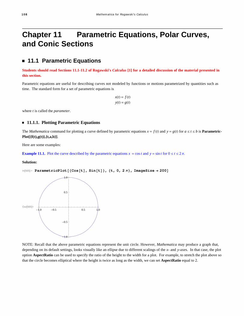
Chapter 11 Parametric Equations, Polar Curves, and Conic Sections
ü 11.1 Parametric Equations
Students should read Sections 11.1-11.2 of Rogawski's Calculus [1] for a detailed discussion of the material presented inthis section.
Parametric equations are useful for describing curves not modeled by functions or motions parametrized by quantities such astime. The standard form for a set of parametric equations is
xt = f tyt = gt
where t is called the parameter.
ü 11.1.1. Plotting Parametric Equations
The Mathematica command for plotting a curve defined by parametric equations x = f t and y = gt for a § t § b is Parametric-
Plot[{f(t),g(t)},{t,a,b}].
Here are some examples:
Example 11.1. Plot the curve described by the parametric equations x = cos t and y = sin t for 0 § t § 2 p.
Solution:
In[565]:= ParametricPlotCost, Sint, t, 0, 2 , ImageSize 200
Out[565]=-1.0 -0.5 0.5 1.0
-1.0
-0.5
0.5
1.0
NOTE: Recall that the above parametric equations represent the unit circle. However, Mathematica may produce a graph that,depending on its default settings, looks visually like an ellipse due to different scalings of the x- and y-axes. In that case, the plot
option AspectRatio can be used to specify the ratio of the height to the width for a plot. For example, to stretch the plot above so
that the circle becomes elliptical where the height is twice as long as the width, we can set AspectRatio equal to 2.
108 Mathematica for Rogawski's Calculus

In[566]:= ParametricPlotCost, Sint, t, 0, 2 , AspectRatio 2, ImageSize 200
Out[566]=-1.0 -0.5 0.5 1.0
-1.0
-0.5
0.5
1.0
Example 11.2. Plot the curve described by the parametric equations x = t2 - 4 and y = t 2 for -2 § t § 3.
Solution: Here is a plot of the curve:
In[567]:= ParametricPlott^2 4, t 2, t, 2, 3
Out[567]=
-4 -2 2 4
-1.0
-0.5
0.5
1.0
1.5
Example 11.3. Plot the curve (prolate cycloid) described by the parametric equations x = 2 q - 4 sin q and y = 2 - 4 cos q for0 § t § 2 p and determine its y-intercepts.
Solution: We first plot the curve:
Chapter 5 109

In[568]:= Clearf, g, f_ 2 4 Sin;
g_ 2 4 Cos;
ParametricPlotf, g, , 4 Pi, 4 Pi,PlotLabel "Prolate cycloid"
Out[571]=
-20 -10 10 20-2
2
4
6Prolate cycloid
To find the y-intercepts (there appears to be two based on the graph), we solve f q = 0 for q:
In[572]:= Solvef 0, Solve::nsmet : This system cannot be solved with the methods available to Solve. à
Out[572]= Solve2 4 Sin 0, Observe that the Solve command here fails to give us an answer since the equation is non-algebraic. However, note that thenegative y-intercept is trivially located at y = -2 corresponding to q = 0. The other (positive) y-intercept must be solved numeri-
cally using the FindRoot command (even the NSolve command fails in this case), where we provide a nearby location (q = p 2)for our desired solution.
In[573]:= root FindRootf 0, , Pi 2Out[573]= 1.89549In[574]:= groot1, 2Out[574]= 3.27609
Thus, the second y-intercept is located approximately at y º f 1.89549 = 3.27609.
NOTE: Observe that we used of the option PlotLabel to print the label "Prolate cycloid" in the plot above. In general, the inside
PlotLabel Ø"text" inside a plot command prints the title text for the given plot.
ü 11.1.2. Parametric Derivatives
Recall that for a curve described by parametric equations x = f t and y = gt, its derivative dy dx can be expressed as a ratiobetween the parametric derivatives dy dt and dx dt (application of the Chain Rule):
dy
dx=
dy
dt
dx
dt
=g' tf ' t
where it is assumed that f ' t ∫ 0.
Example 11.4. Consider the following parametric equations (folium of Descartes):
x = 4 t
1+t3 and y = 4 t2
1+t3
a) Plot the curve described by the parametric equations above (select an appropriate interval for t that captures all the salientfeatures of the graph).b) Find all points of horizontal tangency on the curve.
110 Mathematica for Rogawski's Calculus

c) Find the derivative at the tip of the folium.
Solution:
a) Here is a plot of the folium of Descartes on the interval 0, 20:In[575]:= Clearf, g, t
ft_ 3 t 1 t^3;
gt_ 3 t^2 1 t^3;
ParametricPlotft, gt, t, 0, 20, PlotRange All, AspectRatio 1,PlotLabel "Folium of Descartes", ImageSize 200
Out[578]=
0.5 1.0 1.5
0.5
1.0
1.5
Folium of Descartes
NOTE: The plot above does not reveal the full graph of the folium. A more complete graph is shown in the following plot. Thedashed line indicates an asymptote. Can you generate a Mathematica plot of it? Can you find an equation of the asymptote (seeExercise 7)? Hint: Beware of the discontinuity at t = -1.
-3 -2 -1 1 2 3
-3
-2
-1
1
2
3Folium of Descartes
b) In order to find points of horizontal tangency, that is, points where the slope of the tangent line is equal to zero, it suffices to
solve dy
dx= 0, or equivalently,
dy
dt= 0 (assuming dx
dt∫ 0). Hence, we evaluate
In[579]:= SolveDgt, t 0, tOut[579]= t 0, t 213, t 213, t 123 213
Chapter 5 111
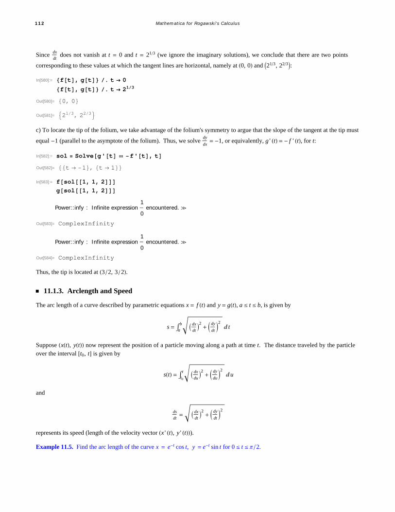
Since dx
dt does not vanish at t = 0 and t = 213 (we ignore the imaginary solutions), we conclude that there are two points
corresponding to these values at which the tangent lines are horizontal, namely at 0, 0 and 213, 223:In[580]:= ft, gt . t 0
ft, gt . t 213
Out[580]= 0, 0Out[581]= 213, 223c) To locate the tip of the folium, we take advantage of the folium's symmetry to argue that the slope of the tangent at the tip must
equal -1 (parallel to the asymptote of the folium). Thus, we solve dy
dx= -1, or equivalently, g ' t = - f ' t, for t:
In[582]:= sol Solveg't f't, tOut[582]= t 1, t 1In[583]:= fsol1, 1, 2
gsol1, 1, 2
Power::infy : Infinite expression 1
0 encountered. à
Out[583]= ComplexInfinity
Power::infy : Infinite expression 1
0 encountered. à
Out[584]= ComplexInfinity
Thus, the tip is located at 3 2, 3 2.
ü 11.1.3. Arclength and Speed
The arc length of a curve described by parametric equations x = f t and y = gt, a § t § b, is given by
s = a
b dx
dt2+ dy
dt2„ t
Suppose xt, yt now represent the position of a particle moving along a path at time t. The distance traveled by the particleover the interval t0, t is given by
st = t0
t dx
du2+ dy
du2„u
and
ds
dt= dx
dt2+ dy
dt2
represents its speed (length of the velocity vector x ' t, y ' t).Example 11.5. Find the arc length of the curve x = e-t cos t, y = e-t sin t for 0 § t § p 2.
112 Mathematica for Rogawski's Calculus

Solution: Here is a plot of the curve:
In[585]:= Clearx, y, txt_ E^t Cost;
yt_ E^t Sint;
ParametricPlotxt, yt, t, 0, Pi 2, ImageSize 250
Out[588]=
0.2 0.4 0.6 0.8 1.0
0.050.100.150.200.250.30
To find its arc length, we compute
In[589]:= 0
2Dxt, t^2 Dyt, t^2 t
Out[589]= 2 1 2In[590]:= NOut[590]= 1.12023
This answer makes sense based on the graph.
Example 11.5. A particle moves along a path described by x = t2 - 4, y = t 2.a) Find the distance traveled by the particle over the interval -3, 3.b) What is the particle's minimum speed over the same interval? When does this occur?
Solution:a) The distance traveled is given by
In[591]:= Clearx, y, txt_ t^2 4;
yt_ t 2;
3
3Dxt, t^2 Dyt, t^2 t
Out[594]=1
812 145 ArcSinh12
In[595]:= NOut[595]= 18.4599
a) We make a plot of the particle's speed:
Chapter 5 113

In[596]:= speed Dxt, t^2 Dyt, t^2Plotspeed, t, 3, 3, ImageSize 250
Out[596]=1
4 4 t2
Out[597]=
-3 -2 -1 1 2 3
1
2
3
4
5
6
This shows that the minimum speed is 1/2 and occurs at t = 0. Can you verify this using calculus techniques?
ü Exercises
In Exercises 1 through 3, sketch the curve represented by the given parametric equations. Be sure to select an appropriateinterval for the parameter that captures all the salient features of the curve.
1. x = t3 , y = t2 2 2. x = 2 q - sin q, y = 1 - cos q 3. x = 3 cos3 q, y = 3 sin3 q
4. Find all points of horizontal and vertical tangency to the curve x = cos q + q sin q, y = sin q - q cos q, 0 § q § 2 p.
5. Consider parametric equations given by x = 3 cos t 3 - cos t and y = 3 sin t 3 - sin t.a) Graph the curve represented by the parametric equations above.b) Find the slope of the line tangent to the curve at the point where t = p 4.c) Find the arc length of the curve from t = 0 to t = 3 p 2.
6. Consider a particle moving along a curve described by x = t - cos t and y = t - sin t with respect to time t.
a) Approximate the distance traveled by the particle over the interval 0, 2 p. Hint: Use the NIntegrate command.b) Find the minimum and maximum speeds of the particle over the same interval. At what times do they occur?
7. Cornu's spiral (also known as Euler's spiral) is a curve defined by the following Fresnel integrals:
xt = 0tcosu2 „u, yt = 0
tsinu2 „u
a) Plot Cornu's spiral for -10 § t § 10.b) Compute the length of Cornu's spiral over the same interval. Then find a formula for the length of Cornu's spiral over theinterval a § t § b.c) Determine the coordinates of the center of the two "eyes" that form Cornu's spiral.
8. Find the asymptote corresponding to the folium of Descartes (see Example 11.4) and plot the asymptote together with thefolium of Descartes.
ü 11.2 Polar Coordinates and Curves
Students should read Sections 11.3-11.4 of Rogawski's Calculus [1] for a detailed discussion of the material presented in
114 Mathematica for Rogawski's Calculus

g pthis section.
Polar coordinates, expressed as r, q), represent the location of a point on the Cartesian plane in terms of distance r from theorigin and angle q with respect to the positive x-axis.
ü 11.2.1. Conversion Formulas
Conversion between Cartesian (rectangular) coordinates x, y and polar coordinates r, q can be achieved by the followingformulas:
r2 = x2 + y2
q = tan-1 y x
x = r cos qy = r sin q
Example 11.6. Perform the following conversions:a) Convert the rectangular coordinates 3, 4 into polar coordinates.b) Convert the polar coordinates 7, p 3 into Cartesian coordinates.
Solution:
a) Using the first set of conversion formulas above, we find that
In[598]:= r 32 42
NArcTan4 3Out[598]= 5
Out[599]= 0.927295
b) This time, we use the second set of conversion formulas:
In[600]:= x 7 CosPi 3y 7 SinPi 3
Out[600]=7
2
Out[601]=7 3
2
ü 11.2.2. Polar Curves
The Mathematica command for plotting a curve described by a polar equation in the form r = f q for a § q § b is Polar-
Plot[f(q),{q, a, b}].
Example 11.7. Plot the graph of the limacon r = 3 - 4 cos q.
Solution: Here is a plot of the limacon:
Chapter 5 115
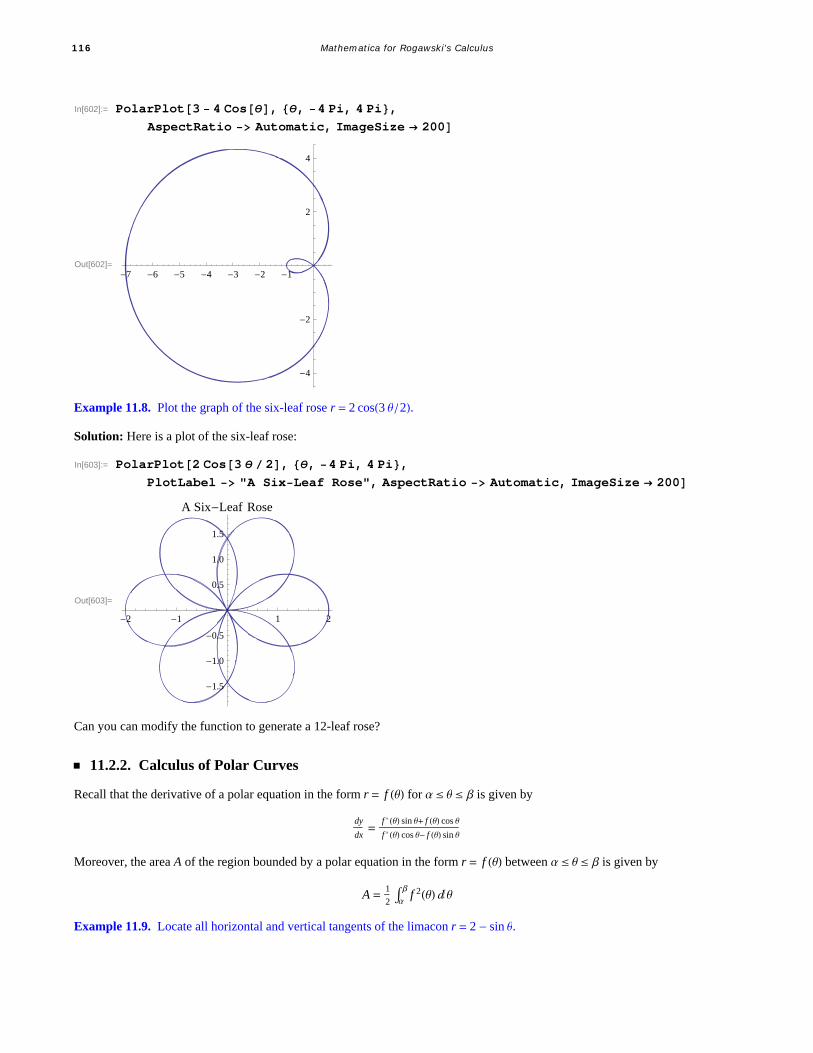
In[602]:= PolarPlot3 4 Cos, , 4 Pi, 4 Pi,
AspectRatio Automatic, ImageSize 200
Out[602]=-7 -6 -5 -4 -3 -2 -1
-4
-2
2
4
Example 11.8. Plot the graph of the six-leaf rose r = 2 cos3 q 2.Solution: Here is a plot of the six-leaf rose:
In[603]:= PolarPlot2 Cos3 2, , 4 Pi, 4 Pi,
PlotLabel "A SixLeaf Rose", AspectRatio Automatic, ImageSize 200
Out[603]=
-2 -1 1 2
-1.5
-1.0
-0.5
0.5
1.0
1.5
A Six-Leaf Rose
Can you can modify the function to generate a 12-leaf rose?
ü 11.2.2. Calculus of Polar Curves
Recall that the derivative of a polar equation in the form r = f q for a § q § b is given by
dy
dx=
f ' q sin q+ f q cos q
f ' q cos q- f q sin q
Moreover, the area A of the region bounded by a polar equation in the form r = f q between a § q § b is given by
A = 1
2 ab f 2q „qExample 11.9. Locate all horizontal and vertical tangents of the limacon r = 2 - sin q.
116 Mathematica for Rogawski's Calculus

Solution: We first plot the limacon to anticipate our solution points:
In[604]:= PolarPlot1 Cos, , 2 Pi, 2 Pi, ImageSize 200
Out[604]=0.5 1.0 1.5 2.0
-1.0
-0.5
0.5
1.0
From the plot above, we should expect to find two horizontal tangents and three vertical tangents.
Next, we compute the derivative of the limacon:
In[605]:= Clearf, f_ 1 Cos
Out[606]= 1 CosIn[607]:= dydx Simplifyf' Sin f Cos f' Cos f Sin
Out[607]= Cos 3
2 Csc
2
1 2 CosTo obtain horizonal tangents, we solve dy dx = 0 for q.
In[608]:= dydx 0
Solvedydx 0,
Out[608]= Cos 3
2 Csc
2
1 2 Cos 0
Solve::ifun : Inverse functions are being used by Solve, so
some solutions may not be found; use Reduce for complete solution information. à
Out[609]= 5
3, ,
3,
3, ,
5
3
Therefore, our two horizontal tangents are located at q = ≤p 3.
As for vertical tangents, we solve for where the reciprocal of the derivative is zero, that is, 1 dy dx = 0 for q.
Chapter 5 117

In[610]:= 1 dydx
Solve1 dydx 0,
Out[610]= 1 2 Cos Sec 3
2 Sin
2
Solve::ifun : Inverse functions are being used by Solve, sosome solutions may not be found; use Reduce for complete solution information. à
Out[611]= 0, 4
3,
2
3,
2
3,
4
3
Since the solution above only gives us the principal solution q = 0 of -tan3 q 2 = 0, we need to additionally solve 3 q 2 = ≤pfor q, which yields our two other solutions, q = ≤2 p 3.
NOTE: What is the derivative at q = p?
Example 11.10. Find the area of the region contained inside the circle r = 3 sin q and outside the convex limacon r = 2 - sin q.
Solution: We first plot the two polar curves on the same set of axes.
In[612]:= PolarPlot3 Sin, 2 Sin, , 0, 2 ,
AspectRatio Automatic, ImageSize 200
Out[612]=-2 -1 1 2
-3
-2
-1
1
2
3
Next, we find their points of intersection by equating them and solving for q:
In[613]:= Solve3 Sin 2 Sin, Solve::ifun : Inverse functions are being used by Solve, so
some solutions may not be found; use Reduce for complete solution information. à
Out[613]=
6
Observe that Mathematica gives only the solution q = p 6, which lies in the first quadrant since trigonometric inverse functionsare involved. We can see from the above graph that the other point of intersection must be at q = 5 p 6 due to symmetry. Thus,the area of the enclosed region is given by the difference in areas enclosed by the circle and limacon between q = p 6 and
118 Mathematica for Rogawski's Calculus

q = 5 p 6:
In[614]:= 1 2 Integrate3 Sin^2, , Pi 6, 5 Pi 6
Integrate2 Sin^2, , Pi 6, 5 Pi 6Out[614]= 3 3
In[615]:= NOut[615]= 5.19615
NOTE: Using even symmetry of our region, it would have been enough to integrate between q = p 6 and q = p 2 and double theresult.
ü Exercises
In Exercises 1 and 2, use Mathematica to perform the following conversions.
1. Convert the rectangular coordinates -1, 3 into polar coordinates.
2. Convert the polar coordinates 5, 3 p 4 into Cartesian coordinates. What if we replace 5, 3 p 4 with -5, 3 p 4?In Exercises 3 through 6, plot the graph of each of the given polar equations and find an interval for q over which each graph istraced only once.3. r = 3 - 4 cos q 4. r = 2 + sin q 5. r = 3 cos 3 q 2 6. r = 5 sin 2 q
7. Generate the butterfly curve r = ‰cos q - 2 cos 4 q + sin5 q 12.8. Find all horizontal and vertical tangents of the lemniscate r2 = cos2 q. Plot its graph to confirm your answers.
9. Consider the rose curve r = cos 2 q for -2 p § q § 2 p.a) Plot its graph.b) Find the area of one petal of the curve.
In Exercises 10 through 12, graph and find the area of each of the given regions.10. The common interior of r = 3 - 2 sin q and r = -3 + 2 sin q.11. Inside r = 2 1 + cos q and outside r = 2 cos q.12. Inner loop of r = 3 + 4 sin q.
In Exercises 13 and 14, find the length of the given curve over the specified interval.13. r = 1 + sin q, 0 § q § 2 p 14. r = 6 1 + cos q, 0 § q § 2 p
15. Consider the polar equations r = 4 sin q and r = 2 2 - sin2 q.a) Graph the polar equations on the same axes.b) Find the points of intersection of the curves.c) Find the circumference of each curve.
ü 11.3 Conic Sections
Students should read Section 11.5 of Rogawski's Calculus [1] for a detailed discussion of the material presented in thissection.
Conic sections refer to the three families of curves (ellipses, hyperbolas, parabolas) generated by intersecting a plane with a cone.Recall the equations for describing each family of curves in standard position:
Chapter 5 119
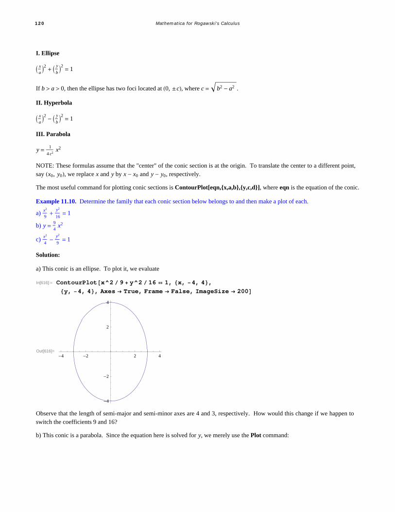
I. Ellipse
x
a2 + y
b2= 1
If b > a > 0, then the ellipse has two foci located at 0, ≤c, where c = b2 - a2 .
II. Hyperbola
x
a2 - y
b2= 1
III. Parabola
y = 1
4 c2x2
NOTE: These formulas assume that the "center" of the conic section is at the origin. To translate the center to a different point,say x0, y0, we replace x and y by x - x0 and y - y0, respectively.
The most useful command for plotting conic sections is ContourPlot[eqn,{x,a,b},{y,c,d}], where eqn is the equation of the conic.
Example 11.10. Determine the family that each conic section below belongs to and then make a plot of each.
a) x2
9+
y2
16= 1
b) y = 9
4x2
c) x2
4-
y2
9= 1
Solution:
a) This conic is an ellipse. To plot it, we evaluate
In[616]:= ContourPlotx^2 9 y^2 16 1, x, 4, 4,y, 4, 4, Axes True, Frame False, ImageSize 200
Out[616]=-4 -2 2 4
-4
-2
2
4
Observe that the length of semi-major and semi-minor axes are 4 and 3, respectively. How would this change if we happen toswitch the coefficients 9 and 16?
b) This conic is a parabola. Since the equation here is solved for y, we merely use the Plot command:
120 Mathematica for Rogawski's Calculus

In[617]:= Plot9 4 x^2, x, 2, 2, ImageSize 200
Out[617]=
-2 -1 1 2
2
4
6
8
c) This conic is a hyperbola. Here is its plot:
In[618]:= ContourPlotx^2 4 y^2 9 1, x, 6, 6,
y, 6, 6, Axes True, Frame False, ImageSize 200
Out[618]=-6 -4 -2 2 4 6
-6
-4
-2
2
4
6
Example 11.11. Find an equation of an ellipse with center at -1, 3 and having semi-major and semi-minor axes of lengths 5and 1/2, respectively.
Solution: From the given data, we see that x0, y0 = -1, 3, a = 5 , and b = 1 2. The equation of our ellipse is therefore:
x+12
5+ 4 y - 32 = 1
To plot it, we evaluate
In[619]:= ContourPlotx 1^2 5 4 y 3^2 1, x, 4, 2, y, 2, 4,AspectRatio 2 3, Axes True, Frame False, ImageSize 200
Out[619]=
-4 -3 -2 -1 1 2
2.5
3.0
3.5
4.0
Chapter 5 121

ü Exercises
In Exercises 1 through 4, plot each of the given conic sections. Can you determine the family that each conic section belongs tobefore plotting? Also, what are the values of the parameters a and b (or c) in each conic section?
1. x2
25+
y2
4= 1 2.
y2
36- x2
16= 1 3. y = 3 x2 4.
y-22
25- x+12
49= 1
5. Consider the ellipse x2
9+ 4 y2 = 1.
a) Make a plot of the ellipse.b) What are the lengths of the semi-major and semi-minor axes?c) Where are the foci located?d) Compute the sum of the distances from the two foci to any point on the ellipse. Do you recognize the answer?
6. Find an equation of an ellipse with center 1 2, -5 and having semi-major and semi-minor axes of lengths 3/4 and 7 ,respectively.
7. Find all points on the hyperbola x2
25-
y2
9= 1 where its slope equals 1.
8. Consider a polar curve of the form r = d e
1+e cos q, where d and e are non-negative constants.
a) Plot this curve for d = 3, and e = 1 2. Do you recognize this curve as a conic section? Of which type? Hint: Use the com-
mand PolarPlot.
b) Repeat part a) but this time use e = 2 instead. Do you recognize this curve as a conic section? Of which type?
c) Repeat part a) but this time use e = 1 instead. Do you recognize this curve as a conic section? Of which type?
d) Describe how the graph changes as we vary the values d and e. What happens to the graph when e = 0? NOTE: The value eis called the eccentricity of the conic section.
e) Assume 0 < e < 1. Convert the polar equation r = d e
1+e cos q to that in standard form for an ellipse, x-x0
a2 + y-y0
b2= 1, and
determine formulas for its center, semi-major, and semi-minor axes. Verify these formulas for the ellipse in part a).
122 Mathematica for Rogawski's Calculus