chapter 8 adaptive control - jccluque.files.wordpress.com · 312 adaptive control chap. 8:...
TRANSCRIPT
Chapter 8Adaptive Control
Many dynamic systems to be controlled have constant or slowly-varying uncertainparameters. For instance, robot manipulators may carry large objects with unknowninertial parameters. Power systems may be subjected to large variations in loadingconditions. Fire-fighting aircraft may experience considerable mass changes as theyload and unload large quantities of water. Adaptive control is a approach to thecontrol of such systems. The basic idea in adaptive control is to estimate the uncertainplant parameters (or, equivalently, the corresponding controller parameters) on-linebased on the measured system signals, and use the estimated parameters in the controlinput computation. An adaptive control system can thus be regarded as a controlsystem with on-line parameter estimation. Since adaptive control systems, whetherdeveloped for linear plants or for nonlinear plants, are inherently nonlinear, theiranalysis and design is intimately connected with the materials presented in this book,and in particular with Lyapunov theory.
Research in adaptive control started in the early 1950's in connection with thedesign of autopilots for high-performance aircraft, which operate at a wide range ofspeeds and altitudes and thus experience large parameter variations. Adaptive controlwas proposed as a way of automatically adjusting the controller parameters in the faceof changing aircraft dynamics. But interest in the subject soon diminished due to thelack of insights and the crash of a test flight. It is only in the last decade that acoherent theory of adaptive control has been developed, using various tools fromnonlinear control theory. These theoretical advances, together with the availability ofcheap computation, have lead to many practical applications, in areas such as robotic
311

312 Adaptive Control Chap. 8
: manipulation, aircraft and rocket control, chemical processes, power systems, shipsteering, and bioengineering.
The objective of this chapter is to describe the main techniques and results inadaptive control. We shall start with intuitive concepts, and then study moresystematically adaptive controller design and analysis for linear and nonlinearsystems. The study in this chapter is mainly concerned with single-input systems.Adaptive control designs for some complex multi-input physical systems are discussedin chapter 9.
8.1 Basic Concepts in Adaptive Control
In this section, we address a few basic questions, namely, why we need adaptivecontrol, what the basic structures of adaptive control systems are, and how to go aboutdesigning adaptive control systems.
8.1.1 Why Adaptive Control ?
In some control tasks, such as those in robot manipulation, the systems to becontrolled have parameter uncertainty at the beginning of the control operation. Unlesssuch parameter uncertainty is gradually reduced on-line by an adaptation or estimationmechanism, it may cause inaccuracy or instability for the control systems. In manyother tasks, such as those in power systems, the system dynamics may have wellknown dynamics at the beginning, but experience unpredictable parameter variationsas the control operation goes on. Without continuous "redesign" of the controller, theinitially appropriate controller design may not be able to control the changing plantwell. Generally, the basic objective of adaptive control is to maintain consistentperformance of a system in the presence of uncertainty or unknown variation in plantparameters. Since such parameter uncertainty or variation occurs in many practicalproblems, adaptive control is useful in many industrial contexts. These include:
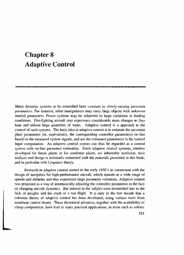
• Robot manipulation: Robots have to manipulate loads of various sizes, weights,and mass distributions (Figure 8.1). It is very restrictive to assume that the inertialparameters of the loads are well known before a robot picks them up and movesthem away. If controllers with constant gains are used and the load parameters arenot accurately known, robot motion can be either inaccurate or unstable. Adaptivecontrol, on the other hand, allows robots to move loads of unknown parameterswith high speed and high accuracy.
Sect. 8.1 Basic Concepts in Adaptive Control 313
• Ship steering: On long courses, ships are usually put under automatic steering.However, the dynamic characteristics of a ship strongly depend on many uncertainparameters, such as water depth, ship loading, and wind and wave conditions(Figure 8.2). Adaptive control can be used to achieve good control performanceunder varying operating conditions, as well as to avoid energy loss due to excessiverudder motion.
• Aircraft control: The dynamic behavior of an aircraft depends on its altitude,speed, and configuration. The ratio of variations of some parameters can liebetween 10 to 50 in a given flight. As mentioned earlier, adaptive control wasoriginally developed to achieve consistent aircraft performance over a large flightenvelope.
• Process control: Models for metallurgical and chemical processes are usuallycomplex and also hard to obtain. The parameters characterizing the processes varyfrom batch to batch. Furthermore, the working conditions are usually time-varying{e.g., reactor characteristics vary during the reactor's life, the raw materialsentering the process are never exactly the same, atmospheric and climaticconditions also tend to -change). In fact, process control is one of the mostimportant and active application areas of adaptive control.
desired trajectoryobstacles
•• unknown load
Figure 8.1 : A robot carrying a load of uncertain mass properties

314 Adaptive Control Chap. 8
Adaptive control has also been applied to other areas, such as power systemsand biomedical engineering. Most adaptive control applications are aimed at handlinginevitable parameter variation or parameter uncertainty. However, in someapplications, particularly in process control, where hundreds of control loops may bepresent in a given system, adaptive control is also used to reduce the number of designparameters to be manually tuned, thus yielding an increase in engineering efficiencyand practicality.
Figure 8.2 : A freight ship under various loadings and sea conditions
To gain insights about the behavior of the adaptive control systems and also toavoid mathematical difficulties, we shall assume the unknown plant parameters areconstant in analyzing the adaptive control designs. In practice, the adaptive controlsystems are often used to handle time-varying unknown parameters. In order for theanalysis results to be applicable to these practical cases, the time-varying plantparameters must vary considerably slower than the parameter adaptation. Fortunately,this is often satisfied in practice. Note that fast parameter variations may also indicatethat the modeling is inadequate and that the dynamics causing the parameter changesshould be additionally modeled.
Finally, let us note that robust control can also be used to deal with parameteruncertainty, as seen in chapter 7. Thus, one may naturally wonder about thedifferences and relations between the robust approach and the adaptive approach. Inprinciple, adaptive control is superior to robust control in dealing with uncertainties inconstant or slowly-varying parameters. The basic reason lies in the learning behaviorof adaptive control systems: an adaptive controller improves its performance asadaptation goes on, while a robust controller simply attempts to keep consistentperformance. Another reason is that an adaptive controller requires little or no apriori information about the unknown parameters, while a robust controller usuallyrequires reasonable a priori estimates of the parameter bounds. Conversely, robustcontrol has some desirable features which adaptive control does not have, such as itsability to deal with disturbances, quickly varying parameters, and unmodeled
1
Sect. 8.1 Basic Concepts in Adaptive Control 315
dynamics. Such features actually may be combined with adaptive control, leading torobust adaptive controllers in which uncertainties on constant or slowly-varyingparameters is reduced by parameter adaptation and other sources of uncertainty arehandled by robustification techniques. It is also important to point out that existingadaptive techniques for nonlinear systems generally require a linear parametrizationof the plant dynamics, i.e., that parametric uncertainty be expressed linearly in termsof a set of unknown parameters. In some cases, full linear parametrization and thusadaptive control cannot be achieved, but robust control (or adaptive control withrobustifying terms) may be possible.
8.1.2 What Is Adaptive Control ?
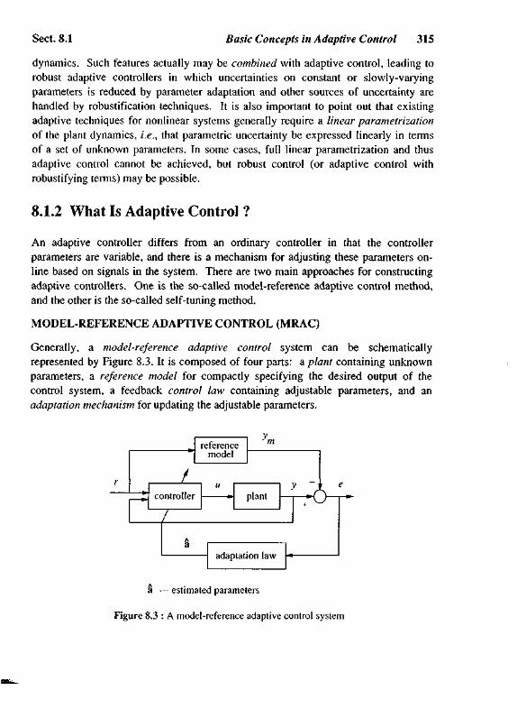
An adaptive controller differs from an ordinary controller in that the controllerparameters are variable, and there is a mechanism for adjusting these parameters on-line based on signals in the system. There are two main approaches for constructingadaptive controllers. One is the so-called model-reference adaptive control method,and the other is the so-called self-tuning method.
MODEL-REFERENCE ADAPTIVE CONTROL (MRAC)
Generally, a model-reference adaptive control system can be schematicallyrepresented by Figure 8.3. It is composed of four parts: a plant containing unknownparameters, a reference model for compactly specifying the desired output of thecontrol system, a feedback control law containing adjustable parameters, and anadaptation mechanism for updating the adjustable parameters.
a — estimated parameters
Figure 8.3 : A model-reference adaptive control system

316 Adaptive Control Chap. 8
The plant is assumed to have a known structure, although the parameters areunknown. For linear plants, this means that the number of poles and the number ofzeros are assumed to be known, but that the locations of these poles and zeros are not.For nonlinear plants, this implies that the structure of the dynamic equations is known,but that some parameters are not.
A reference model is used to specify the ideal response of the adaptive controlsystem to the external command. Intuitively, it provides the ideal plant responsewhich the adaptation mechanism should seek in adjusting the parameters. The choiceof the reference model is part of the adaptive control system design. This choice has tosatisfy two requirements. On the one hand, it should reflect the performancespecification in the control tasks, such as rise time, settling time, overshoot orfrequency domain characteristics. On the other hand, this ideal behavior should beachievable for the adaptive control system, i.e., there are some inherent constraints onthe structure of the reference model (e.g., its order and relative degree) given theassumed structure of the plant model.
The controller is usually parameterized by a number of adjustable parameters(implying that one may obtain a family of controllers by assigning various values tothe adjustable parameters). The controller should have perfect tracking capacity inorder to allow the possibility of tracking convergence. That is, when the plantparameters are exactly known, the corresponding controller parameters should makethe plant output identical to that of the reference model. When the plant parametersare not known, the adaptation mechanism will adjust the controller parameters so thatperfect tracking is asymptotically achieved. If the control law is linear in terms of theadjustable parameters, it is said to be linearly parameterized. Existing adaptivecontrol designs normally require linear parametrization of the controller in order toobtain adaptation mechanisms with guaranteed stability and tracking convergence.
The adaptation mechanism is used to adjust the parameters in the control law.In MRAC systems, the adaptation law searches for parameters such that the responseof the plant under adaptive control becomes the same as that of the reference model,i.e., the objective of the adaptation is to make the tracking error converge to zero.Clearly, the main difference from conventional control lies in the existence of thismechanism. The main issue in adaptation design is to synthesize an adaptationmechanism which will guarantee that the control system remains stable and thetracking error converges to zero as the parameters are varied. Many formalisms innonlinear control can be used to this end, such as Lyapunov theory, hyperstabilitytheory, and passivity theory. Although the application of one formalism may be moreconvenient than that of another, the results are often equivalent. In this chapter, weshall mostly use Lyapunov theory. J

Sect. 8.1 Basic Concepts in Adaptive Control 317
As an illustration of MRAC control, let us describe a simple adaptive controlsystem for an unknown mass.
Example 8.1: MRAC control of an unknown mass
Consider the control of a mass on a frictionless surface by a motor force w, with the plant
dynamics being
mx = u (8.1)
Assume that a human operator provides the positioning command r(t) to the control system
(possibly through a joystick). A reasonable way of specifying the ideal response of the controlled
mass to the external command r(t) is to use the following reference model
with the positive constants Xi and "k^ chosen to reflect the performance specifications, and the
reference model output xm being the ideal output of the control system (i.e., ideally, the mass
should go to the specified position r{t) like a well-damped mass-spring-damper system).
If the mass m is known exactly, we can use the following control law to achieve perfect
tracking
u = m(xm — 2Xx — X2x)
with x = x(t) - xm(t) representing the tracking error and X a strictly positive number. This control
law leads to the exponentially convergent tracking error dynamics
x + 2Xx + X2x = 0
Now let us assume that the mass is not known exactly. We may use the following control law
u = m(xm-2Xic-X2x) (8.3)
which contains the adjustable parameter m. Substitution of this control law into the plant
dynamics leads to the closed-loop error dynamics
mv (8.4)
where s, a combined tracking error measure, is defined by
s = i + Xx (8.5)
the signal quantity v by
v = xm -2Xx -X2x
and the parameter estimation error m by

318 Adaptive Control Chap. 8
fh = m-m
Equation (8.4) indicates that the combined tracking error s is related to the parameter error
through a stable filter relation.
to use the following update law
through a stable filter relation. One way of adjusting parameter m (for reasons to be seen later) is
m = -yvs (8.6)
where y is a positive constant called the adaptation gain. One easily sees the nonlinear nature of
the adaptive control system, by noting that the parameter m is adjusted based on system signals,
and thus the controller (8.3) is nonlinear.
The stability and convergence of this adaptive control system can be analyzed using
Lyapunov theory. For the closed-loop dynamics (8.4) and (8.6), with s and m as states, we can
consider the following Lyapunov function candidate,
V = -[ms2+-m2] (8.7)2 7
Its derivative can be easily shown to be
V = -Xms2 (8.8)
Using Barbalat's lemma in chapter 4, one can easily show that s converges to zero. Due to the
relation (8.5), the convergence of s to zero implies that of the position tracking error x and the
velocity tracking error x.
For illustration, simulations of this simple adaptive control system are provided in Figures
8.4 and 8.5. The true mass is assumed to be m=2. The initial value of m is chosen to be zero,
indicating no a priori parameter knowledge. The adaptation gain is chosen to be y = 0.5, and the
other design parameters are taken to be X^ = 10, Xj = 25, X. = 6. Figure 8.4 shows the results
when the commanded position is r(t) = 0, with initial conditions being x(0) = xm(Q) — 0 and
x(0) = xm(0) = 0.5. Figure 8.5 shows the results when the desired position is a sinusoidal signal,
r(i) = sin(4 t). It is clear that the position tracking errors in both cases converge to zero, while the
parameter error converge to zero only for the latter case. The reason for the non-convergence of
parameter error in the first case can be explained by the simplicity of the tracking task: the
asymptotic tracking of xm(t) can be achieved by many possible values of the estimated parameter
m, besides the true parameter. Therefore, the parameter adaptation law does not bother to find out
the true parameter. On the other hand, the convergence of the parameter error in Figure 8.5 is
because of the complexity of the tracking task, i.e., tracking error convergence can be achieved
only when the true mass is used in the control law. One may examine Equation (8.4) to see the
mathematical evidence for these statements (also see Exercise 8.1). It is also helpful for the
readers to sketch the specific structure of this adaptive mass control system. A more detailed
discussion of parameter convergence is provided in section 8.2. D
1

Sect. 8.1 Basic Concepts in Adaptive Control 319
Ito
0.6
°-50.4
0-3
0.2
0.1
0.0
-0.1
2.5
UIIJ
<u
ter
para
mel
2.0
1.5
1.0
0.5
0.0 0.5 1.0 1.5 2.0 2.5 3.0time(sec)
0.00.0 0.5 1.0 1.5 2.0 2.5 3.0
time(sec)
Figure 8.4 : Tracking Performance and Parameter Estimation for an Unknown Mass,
0.8
0.6
0.4
0.2
0.0
-0.2
-0.4
-0.6
-0.80.0 0.5 1.0 1.5 2.0 2.5 3.0
time(sec)
0.00.0 0.5 1.5 2.0 2.5 3.0
time(sec)
Figure 8.5 : Tracking Performance and Parameter Estimation for an Unknown Mass,
SELF-TUNING CONTROLLERS (STC)
In non-adaptive control design (e.g., pole placement), one computes the parameters ofthe controllers from those of the plant. If the plant parameters are not known, it isintuitively reasonable to replace them by their estimated values, as provided by aparameter estimator. A controller thus obtained by coupling a controller with an on-line (recursive) parameter estimator is called a self-tuning controller. Figure 8.6illustrates the schematic structure of such an adaptive controller. Thus, a self-tuningcontroller is a controller which performs simultaneous identification of the unknownplant.
The operation of a self-tuning controller is as follows: at each time instant, theestimator sends to the controller a set of estimated plant parameters (a in Figure 8.6),

320 Adaptive Control Chap. 8
which is computed based on the past plant input u and output y; the computer finds thecorresponding controller parameters, and then computes a control input u based on thecontroller parameters and measured signals; this control input u causes a new plantoutput to be generated, and the whole cycle of parameter and input updates isrepeated. Note that the controller parameters are computed from the estimates of theplant parameters as if they were the true plant parameters. This idea is often called thecertainty equivalence principle.
controller plant
estimator
S — estimated parameters
Figure 8.6 : A self-tuning controller
Parameter estimation can be understood simply as the process of finding a set ofparameters that fits the available input-output data from a plant. This is different fromparameter adaptation in MRAC systems, where the parameters are adjusted so that thetracking errors converge to zero. For linear plants, many techniques are available toestimate the unknown parameters of the plant. The most popular one is the least-squares method and its extensions. There are also many control techniques for linearplants, such as pole-placement, PID, LQR (linear quadratic control), minimumvariance control, or H°° designs. By coupling different control and estimationschemes, one can obtain a variety of self-tuning regulators. The self-tuning methodcan also be applied to some nonlinear systems without any conceptual difference.
In the basic approach to self-tuning control, one estimates the plant parametersand then computes the controller parameters. Such a scheme is often called indirectadaptive control, because of the need to translate the estimated parameters intocontroller parameters. It is possible to eliminate this part of the computation. To dothis, one notes that the control law parameters and plant parameters are related to eachother for a specific control method. This implies that we may reparameterize the plantmodel using controller parameters (which are also unknown, of course), and then usestandard estimation techniques on such a model. Since no translation is needed in thisscheme, it is called a direct adaptive control scheme. In MRAC systems, one can

Sect. 8.1 Basic Concepts in Adaptive Control 321
similarly consider direct and indirect ways of updating the controller parameters.
Example 8.2 : Self-tuning control of the unknown mass
Consider the self-tuning control of the mass of Example 8.1. Let us still use the pole-placement
(placing the poles of the tracking error dynamics) control law (8.3) for generating the control
input, but let us now generate the estimated mass parameter using an estimation law.
Assume, for simplicity, that the acceleration can be measured by an accelerometer. Since the
only unknown variable in Equation (8.1) is m, the simplest way of estimating it is to simply
divide the control input u{t) by the acceleration x , i.e.,
m(t) = ^ (8.9)x
However, this is not a good method because there may be considerable noise in the measurement
x, and, furthermore, the acceleration may be close to zero. A better approach is to estimate the
parameter using a least-squares approach, i.e., choosing the estimate in such a way that the total
prediction error
J=!e2(r)dr (8.10)
is minimal, with the prediction error e defined as
e{t) = m(t)x(t)-u(f)
The prediction error is simply the error in fitting the known input u using the estimated parameter
m. This total error mini:
The resulting estimate is
m. This total error minimization can potentially average out the effects of measurement noise.
wudr•*o
f w2dr
(8.11)
with w = 'x. If, actually, the unknown parameter m is slowly time-varying, the above estimate has
to be recalculated at every new time instant. To increase computational efficiency, it is desirable
to adopt a recursive formulation instead of repeatedly using (8.11). To do this, we define
P(t) = ~ (8.12)
f wzdr* o
The function P(t) is called the estimation gain, and its update can be directly obtained by using
322 Adaptive Control Chap. 8
i[P-']=w2 (8.13)at
Then, differentiation of Equation (8.11) (which can be written P ~ ' m= f w u dr ) leads to}o
m = -P(t)we (8.14)
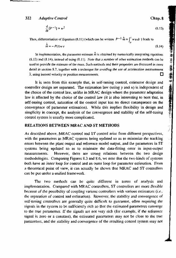
In implementation, the parameter estimate m is obtained by numerically integrating equations
(8.13) and (8.14), instead of using (8.11). Note that a number of other estimation methods can be
used to provide the estimate of the mass. Such methods and their properties are discussed in more
detail in section 8.7, together with a technique for avoiding the use of acceleration measurement
x, using instead velocity or position measurements. Q
It is seen from this example that, in self-tuning control, estimator design andcontroller design are separated. The estimation law (using y and u) is independent ofthe choice of the control law, unlike in MRAC design where the parameter adaptationlaw is affected by the choice of the control law (it is also interesting to note that, inself-tuning control, saturation of the control input has no direct consequence on theconvergence of parameter estimation). While this implies flexibility in design andsimplicity in concept, the analysis of the convergence and stability of the self-tuningcontrol system is usually more complicated.
RELATIONS BETWEEN MRAC AND ST METHODS
As described above, MRAC control and ST control arise from different perspectives,with the parameters in MRAC systems being updated so as to minimize the trackingerrors between the plant output and reference model output, and the parameters in STsystems being updated so as to minimize the data-fitting error in input-outputmeasurements. However, there are strong relations between the two designmethodologies. Comparing Figures 8.3 and 8.6, we note that the two kinds of systemsboth have an inner loop for control and an outer loop for parameter estimation. Froma theoretical point of view, it can actually be shown that MRAC and ST controllerscan be put under a unified framework.
The two methods can be quite different in terms of analysis andimplementation. Compared with MRAC controllers, ST controllers are more flexiblebecause of the possibility of coupling various controllers with various estimators (i.e.,the separation of control and estimation). However, the stability and convergence ofself-tuning controllers are generally quite difficult to guarantee, often requiring thesignals in the system to be sufficiently rich so that the estimated parameters convergeto the true parameters. If the signals are not very rich (for example, if the referencesignal is zero or a constant), the estimated parameters may not be close to the truepamareters, and the stability and convergence of the resulting control system may not
1

Sect. 8.1 Basic Concepts in Adaptive Control 323
be guaranteed. In this situation, one must either introduce perturbation signals in theinput, or somehow modify the control law. In MRAC systems, however, the stabilityand tracking error convergence are usually guaranteed regardless of the richness of thesignals.
Historically, the MRAC method was developed from optimal control ofdeterministic servomechanisms, while the ST method evolved from the study ofstochastic regulation problems. MRAC systems have usually been considered incontinuous-time form, and ST regulators in discrete time-form. In recent years,discrete-time version of MRAC controllers and continuous versions of ST controllershave also been developed. In this chapter, we shall mostly focus on MRAC systems incontinuous form. Methods for generating estimated parameters for self-tuning controlare discussed in section 8.7.
8.1.3 How To Design Adaptive Controllers ?
In conventional (non-adaptive) control design, a controller structure {e.g., poleplacement) is chosen first, and the parameters of the controller are then computedbased on the known parameters of the plant. In adaptive control, the major differenceis that the plant parameters are unknown, so that the controller parameters have to beprovided by an adaptation law. As a result, the adaptive control design is moreinvolved, with the additional needs of choosing an adaptation law and proving thestability of the system with adaptation.
The design of an adaptive controller usually involves the following three steps:
• choose a control law containing variable parameters
• choose an adaptation law for adjusting those parameters
• analyze the convergence properties of the resulting control system
These steps are clearly seen in Example 8.1.
When one uses the self-tuning approach for linear systems, the first two stepsare quite straightforward, with inventories of control and adaptation (estimation) lawsavailable. The difficulty lies in the analysis. When one uses MRAC design, theadaptive controller is usually found by trial and error. Sometimes, the three steps arecoordinated by the use of an appropriate Lyapunov function, or using some symbolicconstruction tools such as the passivity formalism. For instance, in designing theadaptive control system of Example 8.1, we actually start from guessing the Lyapunovfunction V (as a representation of total error) in (8.7) and choose the control and

324 Adaptive Control Chap. 8 | |
adaptation laws so that V decreases. Generally, the choices of control and adaptationlaws in MRAC can be quite complicated, while the analysis of the convergenceproperties are relatively simple.
Before moving on to the application of the above procedure to adaptive controldesign for specific systems, let us derive a basic lemma which will be very useful inguiding our choice of adaptation laws for MRAC systems.
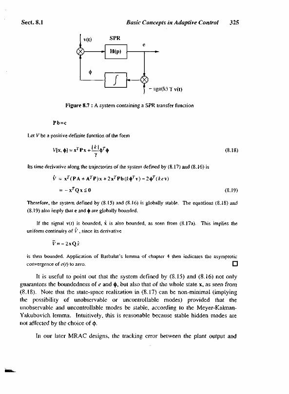
Lemma 8.1: Consider two signals e and <|> related by the following dynamic equation
(8.15)
where e(t) is a scalar output signal, H(p) is a strictly positive real transfer function, kis an unknown constant with known sign, §(t) is a mxl vector function of time, and\(f) is a measurable mxl vector. If the vector § varies according to
<j>(0 = -sgn(£)yev(0 (8.16)
with y being a positive constant, then e(t) and §(t) are globally bounded. Furthermore,if\ is bounded, then
e(t) -> 0 as t -> oo
Note that while (8.15) involves a mixture of time-domain and frequency-domainnotations (with p being the Laplace variable), its meaning is clear: e(t) is the responseof the linear system of SPR transfer function H(p) to the input [k$T(t)\(t)] (witharbitrary initial conditions). Such hybrid notation is common in the adaptive controlliterature, and later on it will save us the definition of intermediate variables.
In words, the above lemma means that if the input signal depends on the outputin the form (8.16), then the whole system is globally stable (i.e., all its states arebounded). Note that this is a feedback system, shown in Figure 8.7, where the plantdynamics, being SPR, have the unique properties discussed in section 4.6.1.
Proof: Let the state-space representation of (8.15) be
x = Ax+b[*<frrvl (8.17a)
e = c r x (8.17b)
Since H(p) is SPR, it follows from the Kalman-Yakubovich lemma in chapter 4 that given a
symmetric positive definite matrix Q, there exists another symmetric positive definite matrix P
such that
A r P + P A = - Q
J
Sect. 8.1 Basic Concepts in Adaptive Control 325
SPR
- sgn(k) y V(t)
Figure 8.7 : A system containing a SPR transfer function
Pb =
Let V be a positive definite function of the form
!A!<|>7> (8.18)
Its time derivative along the trajectories of the system defined by (8.17) and (8.16) is
V =
= -xrQx<0 (8.19)
Therefore, the system defined by (8.15) and (8.16) is globally stable. The equations (8.18) and
(8.19) also imply that e and (|> are globally bounded.
If the signal v(/) is bounded, x is also bounded, as seen from (8.17a). This implies the
uniform continuity of V, since its derivative
is then bounded. Application of Barbalat's lemma of chapter 4 then indicates the asymptotic
convergence of e(l) to zero. CI
It is useful to point out that the system defined by (8.15) and (8.16) not onlyguarantees the boundedness of e and <j>, but also that of the whole state x, as seen from(8.18). Note that the state-space realization in (8.17) can be non-minimal (implyingthe possibility of unobservable or uncontrollable modes) provided that theunobservable and uncontrollable modes be stable, according to the Meyer-Kalman-Yakubovich lemma. Intuitively, this is reasonable because stable hidden modes arenot affected by the choice of $.
In our later MRAC designs, the tracking error between the plant output and

326 Adaptive Control Chap. 8
reference model output will often be related to the parameter estimation errors by anequation of the form (8.15). Equation (8.16) thus provides a technique for adjustingthe controller parameters while guaranteeing system stability. Clearly, the tracking-error dynamics in (8.4) satisfy the conditions of Lemma 8.1 and the adaptation law isin the form of (8.16).
8.2 Adaptive Control of First-Order Systems
Let us now discuss the adaptive control of first-order plants using the MRAC method,as an illustration of how to design and analyze an adaptive control system. Thedevelopment can also have practical value in itself, because a number of simplesystems of engineering interest may be represented by a first-order model. Forexample, the braking of an automobile, the discharge of an electronic flash, or theflow of fluid from a tank may be approximately represented by a first-orderdifferential equation
y = -apy + bpu (8.20)
where y is the plant output, u is its input, and ap and bp are constant plant parameters.
PROBLEM SPECIFICATION
In the adaptive control problem, the plant parameters ap and bp are assumed to beunknown. Let the desired performance of the adaptive control system be specified bya first-order reference model
where am and bm are constant parameters, and r(t) is a bounded external referencesignal. The parameter am is required to be strictly positive so that the reference modelis stable, and bm is chosen strictly positive without loss of generality. The referencemodel can be represented by its transfer function M
where
M =
with p being the Laplace variable. Note that M is a SPR function.
The objective of the adaptive control design is to formulate a control law, and
i

Sect. 8.2 Adaptive Control of First-Order Systems 327
an adaptation law, such that the resulting model following error y{t) - ym
asymptotically converges to zero. In order to accomplish this, we have to assume thesign of the parameter b to be known. This is a quite mild condition, which is oftensatisfied in practice. For example, for the braking of a car, this assumption amounts tothe simple physical knowledge that braking slows down the car.
CHOICE OF CONTROL LAW
As the first step in the adaptive controller design, let us choose the control law to be
u= ar(t)r + ay(t)y (8.22)
where ar and ay are variable feedback gains. With this control law, the closed-loopdynamics are
y = -(ap-aybp)y + arbpr{t) (8.23)
The reason for the choice of control law in (8.22) is clear: it allows thepossibility of perfect model matching. Indeed, if the plant parameters were known, thefollowing values of control parameters
ar =— a =^— (8.24)bp bp
would lead to the closed-loop dynamics
which is identical to the reference model dynamics, and yields zero tracking error. Inthis case, the first term in (8.22) would result in the right d.c. gain, while the secondterm in the control law (8.22) would achieve the dual objectives of canceling the term(- ay) in (8.20) and imposing the desired pole —amy.
In our adaptive control problem, since a and bp are unknown, the control inputwill achieve these objectives adaptively, i.e., the adaptation law will continuouslysearch for the right gains, based on the tracking error y - ym , so as to make y tend toym asymptotically. The structure of the adaptive controller is illustrated in Figure 8.8.
CHOICE OF ADAPTATION LAW
Let us now choose the adaptation law for the parameters ar and ay. Let
e=y-ym
be the tracking error. The parameter errors are defined as the difference between the

328 Adaptive Control Chap. 8
Figure 8.8 : A MRAC system for the first-order plant
controller parameter provided by the adaptation law and the ideal parameters, i.e.,
5(0 =.ar
ay
"A *"ar-arA *
ay-ay
(8.25)
The dynamics of tracking error can be found by subtracting (8.23) from (8.21),
b a )y + (b ar - bm)r
= - ame + bp(arr + ayy)
This can be conveniently represented as
e =bD ~ ~ 1 ~
—i—(arr+ayy) = —M(arr
(8.26)
(8.27)
with p denoting the Laplace operator.
Relation (8.27) between the parameter errors and tracking error is in the familiarform given by (8.15). Thus, Lemma 8.1 suggests the following adaptation law
ar = - sgn(bp) yer
a =-sgn(b )yey
(8.28a)
(8.28b)
with y being a positive constant representing the adaptation gain. From (8.28), it isseen that sgn(fe ) determines the direction of the search for the proper controllerparameters.

Sect. 8.2 Adaptive Control of First-Order Systems 329
TRACKING CONVERGENCE ANALYSIS
With the control law and adaptation law chosen above, we can now analyze thesystem's stability and convergence behavior using Lyapunov theory, or equivalentlyLemma 8.1. Specifically, the Lyapunov function candidate
V(e, *) = I e2 + 1 \bp\(a2 + ay
2) (8.29)
can be easily shown to have the following derivative along system trajectories
V=-a e2
Thus, the adaptive control system is globally stable, i.e., the signals e, ar and a arebounded. Furthermore, the global asymptotic convergence of the tracking error e{t) isguaranteed by Barbalat's lemma, because the boundedness of e, ar and ay implies theboundedness of e (according to (8.26)) and therefore the uniform continuity of V.
It is interesting to wonder why the adaptation law (8.28) leads to tracking errorconvergence. To understand this, let us see intuitively how the control parametersshould be changed. Consider, without loss of generality, the case of a positivesgn(&A Assume that at a particular instant t the tracking error e is negative,indicating that the plant output is too small. From (8.20), the control input u should beincreased in order to increase the plant output. From (8.22), an increase of the controlinput u can be achieved by increasing ar (assuming that r{t) is positive). Thus, theadaptation law, with the variation rate of ar depending on the product of sgn(£>), r ande, is intuitively reasonable. A similar reasoning can be made about ay .
The behavior of the adaptive controller is demonstrated in the followingsimulation example.
Example 8.3: A first-order plant
Consider the control of the unstable plant
y = y + 3«
using the previously designed adaptive controller. The plant parameters a =-l,b = 3 are
assumed to be unknown to the adaptive controller. The reference model is chosen to be
i.e., am = 4, bm = 4. The adaptation gain y is chosen to be equal to 2. The initial values of both
parameters of the controller are chosen to be 0, indicating no a priori knowledge. The initial
conditions of the plant and the model are both zero.

330 Adaptive Control
Two different reference signals are used in the simulation:
Chap. 8
•ga.DO
5.0 r
3.53.02.52.01.51.00.50.0
0.0
• lit) = 4. It is seen from Figure 8.9 that the tracking error converges to zero but the
parameter error does not.
• r(t) - 4 sin(3 f). It is seen from Figure 8.10 that both the tracking error and
parameter error converge to zero. D
1.0 2.0 3.0 4.0 5.0time(sec)
2.0
1.5
1.0
0.5
0.0
g -0-5°- -1.0
-1.5
-2.00.0 1.0 2.0 3.0 4.0 5.0
time(sec)
Figure 8.9 : Tracking performance and parameter estimation, r(t) = 4
2.0 4.0 6.0 8.0 10.0time(sec)
2.0
1.5
1.0
0.5
0.0
-0.5
-1.0
-1.5
-2.00.0 2.0 4.0 6.0 8.0 10.0
time(sec)
Figure 8.10 : Tracking performance and parameter estimation, r(t) = 4 sin(31)
Note that, in the above adaptive control design, although the stability andconvergence of the adaptive controller is guaranteed for any positive j , am and bm , theperformance of the adaptive controller will depend critically on y. If a small gain ischosen, the adaptation will be slow and the transient tracking error will be large.Conversely, the magnitude of the gain and, accordingly, the performance of theadaptive control system, are limited by the excitation of unmodeled dynamics, becausetoo large an adaptation gain will lead to very oscillatory parameters.

Sect. 8.2 Adaptive Control of First-Order Systems 331
PARAMETER CONVERGENCE ANALYSIS
In order to gain insights about the behavior of adaptive control system, let usunderstand the convergence of estimated parameters. From the simulation results ofExample 8.3, one notes that the estimated parameters converge to the exact parametervalues for one reference signal but not for the other. This prompts us to speculate arelation between the features of the reference signals and parameter convergence, i.e.,the estimated parameters will not converge to the ideal controller parameters unlessthe reference signal r(t) satisfies certain conditions.
Indeed, such a relation between the features of reference signal andconvergence of estimated parameters can be intuitively understood. In MRACsystems, the objective of the adaptation mechanism is to find out the parameters whichdrive the tracking error y - ym to zero. If the reference signal r(t) is very simple, suchas a zero or a constant, it is possible for many vectors of controller parameters, besidesthe ideal parameter vector, to lead to tracking error convergence. Then, the adaptationlaw will not bother to find out the ideal parameters. Let Q. denote the set composed ofall the parameter vectors which can guarantee tracking error convergence for aparticular reference signal history r(t). Then, depending on the initial conditions, thevector of estimated parameters may converge to any point in the set or wonder aroundin the set instead of converging to the true parameters. However, if the referencesignal r(t) is so complex that only the true parameter vector a* = \a* ay*]T can leadto tracking error convergence, then we shall have parameter convergence.
Let us now find out the exact conditions for parameter convergence. We shalluse simplified arguments to avoid tedious details. Note that the output of the stablefilter in (8.27) converges to zero and that its input is easily shown to be uniformlycontinuous. Thus, arr + ayy must converge to zero. From the adaptation law (8.28)and the tracking error convergence, the rate of the parameter estimates converges tozero. Thus, when time t is large, a is almost constant, and
i.e.,
vT(t) 2 = 0 (8.30)
with
v = [r y]T a = [a,. ayf
Here we have one equation (with time-varying coefficients) and two variables. Theissue of parameter convergence is reduced to the question of what conditions the

332 Adaptive Control Chap. 8
vector [r(t) y(t)]T should satisfy in order for the equation to have a unique zerosolution.
If r(f) is a constant r0 , then for large t,
with a being the d.c. gain of the reference model. Thus,
[r y] = U «]r0
Equation (8.30) becomes
ar + aa = 0
Clearly, this implies that the estimated parameters, instead of converging to zero,converge to a straight line in parameter space. For Example 8.3, with a = 1, the aboveequation implies that the steady state errors of the two parameters should be of equalmagnitudes but opposite signs. This is obviously confirmed in Figure 8.9.
However, when r{t) is such that the corresponding signal vector v(t) satisfies theso called "persistent excitation" condition, we can show that (8.28) will guaranteeparameter convergence. By persistent excitation of v, we mean that there exist strictlypositive constants ccj and T such that for any t > 0,
' + r a 1 l (8.31)
To show parameter convergence, we note that multiplying (8.30) by v(0 andintegrating the equation for a period of time T, leads to
Ct + T T ~
vv J dra = 0
Condition (8.31) implies that the only solution of this equation is a = 0, i.e., parametererror being zero. Intuitively, the persistent excitation of v(f) implies that the vectorsv(f) corresponding to different times t cannot always be linearly dependent.
The only remaining question is the relation between r(t) and the persistentexcitation of \(t). One can easily show that, in the case of the first order plant, thepersistent excitation of v can be guaranteed, if r(t) contains at least one sinusoidalcomponent.

Sect. 8.2 Adaptive Control of First-Order Systems 333
EXTENSION TO NONLINEAR PLANTS
The same method of adaptive control design can be used for the nonlinear first-orderplant described by the differential equation
y = -apy-cpf(y) + bpu (8.32)
where / is any known nonlinear function. The nonlinearity in these dynamics ischaracterized by its linear parametrization in terms of the unknown constant c. Insteadof using the control law (8.22), we now use the control law
u = ayy + aff(y) + arr (8.33)
where the second term is introduced with the intention of adaptively canceling thenonlinear term.
Substituting this control law into the dynamics (8.32) and subtracting theresulting equation by (8.21), we obtain the error dynamics
1 ~e = —M( ayy + aff(y) + arr)
kr
where the parameter error 5yis defined as
~ A cp
By choosing the adaptation lawA
ay = -sgn(bp)yey (8.34a)
af= ~sgn(bp)yef (8.34b)
ar - -sgn(bp)yer (8.34c)one can similarly show that the tracking error e converges to zero, and the parametererror remains bounded.
As for parameter convergence, similar arguments as before can reveal theconvergence behavior of the estimated parameters. For constant reference inputr = r0, the estimated parameters converge to the line (with a still being the d.c. gain ofthe reference model)
=0
which is a straight line in the three-dimensional parameter space. In order for the

334 Adaptive Control Chap. 8
parameters to converge to the ideal values, the signal vector v = [r(t) y(t) f(y)]T
should be persistently exciting, i.e., there exists positive constants ocj and T such thatfor any time f > 0,
,r+r\vTdr> a, I
Generally speaking, for linear systems, the convergent estimation of mparameters require at least m/2 sinusoids in the reference signal r(t), as will bediscussed in more detail in sections 8.3 and 8.4. However, for this nonlinear case,such simple relation may not be valid. Usually, the qualitative relation between r{t)and v(0 is dependent on the particular nonlinear functions/(y). It is unclear how manysinusoids in r(t) are necessary to guarantee the persistent excitation of v(t).
The following example illustrates the behavior of the adaptive system for anonlinear plant.
Example 8.4: simulation of a first-order nonlinear plant
Assume that a nonlinear plant is described by the equation
y- (8.35)
This differs from the unstable plant in Example 8.3 in that a quadratic term is introduced in the
plant dynamics.
Let us use the same reference model, initial parameters, and design parameters as in Example
8.3. For the reference signal r(r) = 4, the results are shown in Figure 8.11. It is seen that the
tracking error converges to zero, but the parameter errors are only bounded. For the reference
signal r(l) = 4sin(3(), the results are shown in Figure 8.12. It is noted that the tracking error and
the parameter errors for the three parameters all converge to zero. LJ
In this example, it is interesting to note two points. The first point is that asingle sinusoidal component in r(t) allows three parameters to be estimated. Thesecond point is that the various signals (including a and y) in this system are muchmore oscillatory than those in Example 8.3. Let us understand why. The basic reasonis provided by the observation that nonlinearity usually generates more frequencies,and thus v(t) may contain more sinusoids than r(t). Specifically, in the above example,with /-(0 = 4sin(31), the signal vector v converges to
v(t) = [r(t) yss(t) fss(t)]
where ysjj) is the steady-state response and fss(t) the corresponding function value,

Sect. 8.3 Adaptive Control of Linear Systems With Full State Feedback 335
o
KO
gper
f
a
ack
£3
5.04.54.03.53.02.52.01.51.00.50.0
0.0 0.5 1.0 1.5 2.0 2.5 3.0time(sec)
1.81.61.41.21.00.80.60.40.20.0 >
0.0 0.5 1.0 1.5 2.0 2.5 3.0time(sec)
o03
ew
eter
U1E
J1
0.20.0
-0.2-0.4-0.6
-L0-1.2-1.4-1.6-1.8
0.0 0.5 1.0 1.5 2.0 2.5 3.0time(sec)
0.40.20.0
-0.2-0.4-0.6-0.8-1.0-1.2-1.4-1.6
0.0 0.5 1.0 1.5 2.0 2.5 3.0time(sec)
Figure 8.11 : Adaptive control of a first-order nonlinear system, r(t) = 4
upper left: tracking performance
upper right: parameter ar ; lower left: parameter a ; lower right: parameter as
fss(t) = yss2 = 16A2sin2(3r + (J>) = 8 A2( 1 - cos(6? •
where A and <|) are the magnitude and phase shift of the reference model at co = 3.Thus, the signal vector v(t) contains two sinusoids, with/(jy) containing a sinusoid attwice the original frequency. Intuitively, this component at double frequency is thereason for the convergent estimation of the three parameters and the more oscillatorybehavior of the estimated parameters.
Adaptive Control of Linear Systems With Full StateFeedback
Let us now move on to adaptive control design for more general systems. In thissection, we shall study the adaptive control of linear systems when the full state ismeasurable. We consider the adaptive control of «th-order linear systems in

336 Adaptive Control Chap. 8
14.0
3.0
2.0
1.0
0.0
-1.0
-2.0
-3.0
-4.00.0 2.0 4.0 6.0 8.0 10.0
time(sec)
1.8
1.6
1.4
1.2
1.0
0.8
0.6
0.4
0.2
0.00.0 2.0 4.0 6.0 8.0 10.0
time(sec)
B -0.5 -
-1.0 -
-1.5 -
-2.06.0 8.0 10.0
time(sec)
0.5
0.0
-0-5
-1.0
-1.50.0 2.0 4.0 6.0 8.0 10.0
time(sec)
Figure 8.12 : Adaptive control of a first-order nonlinear system, r{t) = 4sin(3t)
upper left: tracking performance
upper right: parameter ar ; lower left: parameter a ; lower right: parameter ay-
companion form:
••••+ ao y = (8.36)
where the state components y,y,... ,y(n~^ are measurable. We assume that thecoefficient vector a = [ an ... aj ao ]T is unknown, but that the sign of an is assumedto be known. An example of such systems is the dynamics of a mass-spring-dampersystem
my + cy + ky = u
where we measure position and velocity (possibly with an optical encoder for positionmeasurement, and a tachometer for velocity measurement, or simply numericallydifferentiate the position signals).
The objective of the control system is to make y closely track the response of astable reference model

Sect. 8.3 Adaptive Control of Linear Systems With Full State Feedback 337
< W f l ) + *n-\ym{n-l) + ••••+ ° w * = >it) (8.37)
with r{t) being a bounded reference signal.
CHOICE OF CONTROL LAW
Let us define a signal z(t) as follows
with Pj,..., fin being positive constants chosen such that pn + fin_ipn~l + .... + Po is astable (Hurwitz) polynomial. Adding (- anz(t)) to both sides of (8.36) andrearranging, we can rewrite the plant dynamics as
Let us choose the control law to be
«= anz + an_x^»-l'> + ....+aoy = \r(t)a(t) (8.39)
where \(t) = [z(t) y("~V ....y y]T and
A , . r A A A A n T
a(t) = [an an_l .... a, a j '
denotes the estimated parameter vector. This represents a pole-placement controllerwhich places the poles at positions specified by the coefficients P,-. The tracking errore = y - ym then satisfies the closed-loop dynamics
an[eW + pn_,eO»-l) + .... + %e] = vT(t) a(r) (8.40)
where~ A
a =a - a
CHOICE OF ADAPTATION LAWLet us now choose the parameter adaptation law. To do this, let us rewrite the closed-loop error dynamics (8.40) in state space form,
k = Ax + b[(l/an)vTa] (8.41a)
e = cx (8.41b)
where

338 Adaptive Control Chap. 8
00
0
"Po
10
0
-Pi
01
0
-P2
. . 0
1
• • - P n - 1
b =
00
01
c = [ l 0 . . 0 0]
Consider the Lyapunov function candidate
where both F and P are symmetric positive definite constant matrices, and P satisfies
PA + ATP = - Q Q = Q r > 0
for a chosen Q. The derivative V can be computed easily as
V = - xrQx + 2aTvbTPx + 2 a r r - l S
Therefore, the adaptation law
a = -TvbrPx (8.42)
leads to
One can easily show the convergence of x using Barbalat's lemma. Therefore, withthe adaptive controller defined by control law (8.39) and adaptation law (8.42), e andits (n-1) derivatives converge to zero. The parameter convergence condition canagain be shown to be the persistent excitation of the vector v. Note that a similardesign can be made for nonlinear systems in the controllability canonical form, asdiscussed in section 8.5.

Sect. 8.4 Adaptive Control of Linear Systems With Output Feedback 339
8.4 Adaptive Control of Linear Systems With OutputFeedback
In this section, we consider the adaptive control of linear systems in the presence ofonly output measurement, rather than full state feedback. Design in this case isconsiderably more complicated than when the full state is available. This partly arisesfrom the need to introduce dynamics in the controller structure, since the output onlyprovides partial information about the system state. To appreciate this need, one cansimply recall that in conventional design (no parameter uncertainty) a controllerobtained by multiplying the state with constant gains (pole placement) can stabilizesystems where all states are measured, while additional observer structures must beused for systems where only outputs are measured.
A linear time-invariant system can be represented by the transfer function
where
... + an_xpn~\ + pn
where kp is called the high-frequency gain. The reason for this term is that the plantfrequency response at high frequency verifies
\W(j<o)\ « —P-
i.e., the high frequency response is essentially determined by kp. The relative degree rof this system is r = n-m. In our adaptive control problem, the coefficients a(-, b:(i = 0, 1,..., n—\;j =0, 1, , m—l) and the high frequency gain kp are all assumed tobe unknown.
The desired performance is assumed to be described by a reference model withtransfer function
Wm(p) = kmZ-p- (8.44)Rm
where Zm and Rm are monic Hurwitz polynomials of degrees nm and mm, and km ispositive. It is well known from linear system theory that the relative degree of the

340 Adaptive Control Chap. 8
reference model has to be larger than or equal to that of the plant in order to allow thepossibility of perfect tracking. Therefore, in our treatment, we will assume thatnm-mm>n-m.
The objective of the design is to determine a control law, and an associatedadaptation law, so that the plant output y asymptotically approaches ym. Indetermining the control input, the output y is assumed to be measured, but nodifferentiation of the output is allowed, so as to avoid the noise amplificationassociated with numerical differentiation. In achieving this design, we assume thefollowing a priori knowledge about the plant:
• the plant order n is known
• the relative degree n- mis known
• the sign of kp is known
• the plant is minimum-phase
Among the above assumptions, the first and the second imply that the modelstructure of the plant is known. The third is required to provide the direction ofparameter adaptation, similarly to (8.28) in section 8.2. The fourth assumption issomewhat restrictive. It is required because we want to achieve convergent tracking inthe adaptive control design. Adaptive control of non-minimum phase systems is still atopic of active research and will not be treated in this chapter.
In section 8.4.1, we discuss output-feedback adaptive control design for linearplants with relative degree one, i.e., plants having one more pole than zeros. Designfor these systems is relatively straightforward. In section 8.4.2, we discuss output-feedback design for plants with higher relative degree. The design andimplementation of adaptive controllers in this case is more complicated because it isnot possible to use SPR functions as reference models.
8.4.1 Linear Systems With Relative Degree One
When the relative degree is 1, i.e., m = n— 1, the reference model can be chosen to beSPR. This choice proves critical in the development of globally convergent adaptivecontrollers.
CHOICE OF CONTROL LAW
To determine the appropriate control law for the adaptive controller, we must firstknow what control law can achieve perfect tracking when the plant parameters are

Sect. 8.4 Adaptive Control of Linear Systems With Output Feedback 341
perfectly known. Many controller structures can be used for this purpose. Thefollowing one, although somewhat peculiar, is particularly convenient for lateradaptation design.
Example 8.5: A controller for perfect tracking
Consider the plant described by
kJp + bn)(8.45)
and the reference model
2P +amlP+am2
r(t)wm(P)
y (t)m
Wp(p)
(8.46)
Figure 8.13 : A model-reference control system for relative degree 1
Let the controller be chosen as shown in Figure 8.13, with the control law being
u = 0CiZ + y + kr (8.47)P + bm
where z = u/(p + bm), i.e., z is the output of a first-order filter with input u, and CX| , p | ,p2 , k are
controller parameters. If we take these parameters to be
P| =_am\-ap\
342 Adaptive Control Chap. 8
kKp
one can straightforwardly show that the transfer function from the reference input r to the plant
output y is
P
Therefore, perfect tracking is achieved with this control law, i.e., y(t) = ym{t), V/ > 0.
It is interesting to see why the closed-loop transfer function can become exactly the same as
that of the reference model. To do this, we note that the control input in (8.47) is composed of
three parts. The first part in effect replaces the plant zero by the reference model zero, since the
transfer function from Mj to y (see Figure 8.13) is
The second part places the closed-loop poles at the locations of those of the reference model.
This is seen by noting that the transfer function from u0 to y is (Figure 8.13)
The third part of the control law (km/kp)r obviously replaces kp , the high frequency gain of the
plant, by km. As a result of the above three parts, the closed-loop system has the desired transfer
function. D
The controller structure shown in Figure 8.13 for second-order plants can beextended to any plant with relative degree one. The resulting structure of the controlsystem is shown in Figure 8.14, where k* , 0j* ,02* and 0O* represents controllerparameters which lead to perfect tracking when the plant parameters are known.
The structure of this control system can be described as follows. The block forgenerating the filter signal ci)[ represents an (« - l) tn order dynamics, which can bedescribed by
(»1 = Aooj + hu
where (Oj is an (n— l)xl state vector, A is an («- l)x(n-1) matrix, and h is a constantvector such that (A, h) is controllable. The poles of the matrix A are chosen to be the

Sect. 8.4 Adaptive Control of Linear Systems With Output Feedback 343
r(t)
Figure 8.14 : A control system with perfect tracking
same as the roots of the polynomial Zm(p), i.e.,
dct[pl-A] =Zm(p)
1 v-
(8.48)
The block for generating the («— l)xl vector oo2 has the same dynamics but with y asinput, i.e.,
d)2 = Aco2 + hy
It is straightforward to discuss the controller parameters in Figure 8.14. The scalargain k* is defined to be
and is intended to modulate the high-frequency gain of the control system. The vector9j* contains (w-1) parameters which intend to cancel the zeros of the plant. Thevector 02* contains (n-1) parameters which, together with the scalar gain 0O* canmove the poles of the closed-loop control system to the locations of the referencemodel poles. Comparing Figure 8.13 and Figure 8.14 will help the reader becomefamiliar with this structure and the corresponding notations.
As before, the control input in this system is a linear combination of thereference signal r(t), the vector signal (al obtained by filtering the control input u, thesignals 0)2 obtained by filtering the plant output y, and the output itself. The controlinput u can thus be written, in terms of the adjustable parameters and the various

344 Adaptive Control Chap. 8
signals, as
u*{t) = k* r + 8 , * « ) 1 + e 2 * a ) 2 + Q*y (8.49)
Corresponding to this control law and any reference input r(t), the output of the plant
is
(8.50)
since these parameters result in perfect tracking. At this point, one easily sees thereason for assuming the plant to be minimum-phase: this allows the plant zeros to becanceled by the controller poles.
In the adaptive control problem, the plant parameters are unknown, and theideal control parameters described above are also unknown. Instead of (8.49), thecontrol law is chosen to be
u = k{t)r + 91(0<»1 + 62(0(»2 + QoW)1 (8-51)
where k(t), 0](O ,92(0 and Q0(t) are controller parameters to be provided by theadaptation law.
CHOICE OF ADAPTATION LAW
For notational simplicity, let 8 be the 2 / ix l vector containing all the controllerparameters, and oo be the 2« x 1 vector containing the corresponding signals, i.e.,
9(0 = WO 6i(f) 92(0 %(t)]T
(o(t) = [r(t) oo,(O oo2(O y(t)]T
Then the control law (8.51) can be compactly written as
u = QT(t)(o{t) (8.52)
Denoting the ideal value of 6 by 0* and the error between 9(0 and 9 by<|>(0 = 9(f) - 9*, the estimated parameters 9(t) can be represented as
9(0 = 9* + (j)(0
Therefore, the control law (8.52) can also be written as
In order to choose an adaptation law so that the tracking error e converges to zero, we
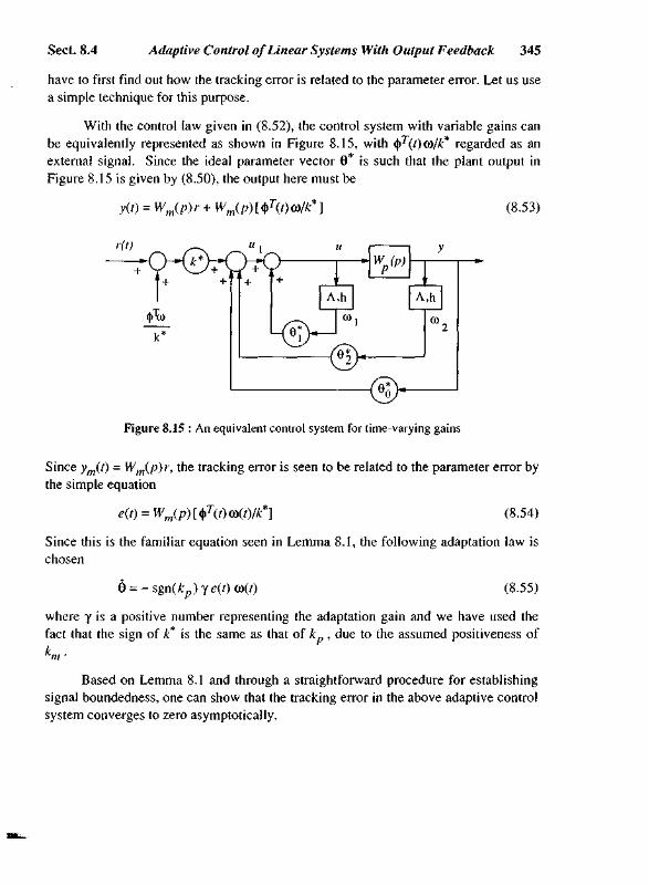
Sect. 8.4 Adaptive Control of Linear Systems With Output Feedback 345
have to first find out how the tracking error is related to the parameter error. Let us usea simple technique for this purpose.
With the control law given in (8.52), the control system with variable gains canbe equivalently represented as shown in Figure 8.15, with <^(t)(o/k* regarded as anexternal signal. Since the ideal parameter vector 0* is such that the plant output inFigure 8.15 is given by (8.50), the output here must be
y(0 = (8.53)
Figure 8.15 : An equivalent control system for time-varying gains
Since ym(t) = Wm{p)r, the tracking error is seen to be related to the parameter error bythe simple equation
e(t) = Wm(p) [§T(t)(o(t)/k*] (8.54)
Since this is the familiar equation seen in Lemma 8.1, the following adaptation law ischosen
= -sgn(k )ye(t)(o(t) (8.55)
where y is a positive number representing the adaptation gain and we have used thefact that the sign of k* is the same as that of k , due to the assumed positiveness of
"w •
Based on Lemma 8.1 and through a straightforward procedure for establishingsignal boundedness, one can show that the tracking error in the above adaptive controlsystem converges to zero asymptotically.

346 Adaptive Control Chap. 8
8.4.2 Linear Systems With Higher Relative Degree
The design of adaptive controller for plants with relative degree larger than 1 is bothsimilar to, and different from, that for plants with relative degree 1. Specifically, thechoice of control law is quite similar but the choice of adaptation law is very different.This difference comes from the fact that the reference model now cannot be SPR.
CHOICE OF CONTROL LAW
We can show that the controller part of the system in Figure 8.15 is also applicable toplants with relative degree larger than 1, leading to exact tracking when the plantparameters are exactly known. Let us again start from a simple example.
Example 8.6: Consider the second order plant described by the transfer function
kpuy=-^—
and the reference model
kmr
which are similar to those in Example 8.5, but now contain no zeros.
Let us consider the control structure shown in Figure 8.16 which is a slight modification of
the controller structure in Figure 8.13. Note that bm in the filters in Figure 8.13 has been replaced
by a positive number Xo . Of course, the transfer functions W and Wm in Figure 8.16 now have
relative degree 2.
The closed-loop transfer function from the reference signal r to the plant output y is
P + K kP
1 + -p + Xo pi + aplp + ap2
Therefore, if the controller parameters ax , P, , $2 > arK^ ^ a r e chosen such that
{p + Xo + a ,) ( p 2 + apXp + ap2) + kp($]P + P2) = {p + \,)(p2 +amlp + am2)
and

Sect. 8.4 Adaptive Control of Linear Systems With Output Feedback 347
r(t)
k+ s
u
a l
P + X0
J
Pjp+P2
P+Xo
wm(P)
Wp(p)
m
y ' •.
Figure 8.16 : A model-reference control system for relative degree 2
then the closed loop transfer function W becomes identically the same as that of the reference
model. Clearly, such choice of parameters exists and is unique. D
For general plants of relative degree larger than 1, the same control structure asgiven in Figure 8.14 is chosen. Note that the order of the filters in the control law isstill ( « - 1). However, since the model numerator polynomial Zm(p) is of degreesmaller than (« - 1), it is no longer possible to choose the poles of the filters in thecontroller so that det[pl - A] = Zm(p) as in (8.48). Instead, we now choose
(8.57)
where X{p) = det[pl - A] and X^(p) is a Hurwitz polynomial of degree (n - 1 - m).With this choice, the desired zeros of the reference model can be imposed.
Let us denote the transfer function of the feedforward part (M/MJ) of thecontroller by X(p)/(k{p) + C(p)), and that of the feedback part by D(p)/X(p), wherethe polynomial C(p) contains the parameters in the vector 0j, and the polynomialD(p) contains 0O and the parameters in the vector 02. Then, the closed-loop transferfunction is easily found to be
W =—ry R
kkpZpXx{p)Zm{P)(8.58)

348 Adaptive Control Chap. 8
The question now is whether in this general case there exist choice of values fork, 60 , 0 ( and 92 such that the above transfer function becomes exactly the same asWm(p), or equivalently
Rp(Up)+ C(p)) + kpZpD{p) = ZpRJp) (8.59)
The answer to this question can be obtained from the following lemma:
Lemma 8.2: Let A{p) and B(p) be polynomials of degree nj and W2» respectively. IfA(p) and B(p) are relatively prime, then there exist polynomials M(p) and N(p) suchthat
A(p)M(p) + B(p)N(p) = A*(p) (8.60)
where A*(p) is an arbitrary polynomial.
This lemma can be used straightforwardly to answer our question regarding(8.59). By regarding Rp as A(p) in the lemma, kpZ as B(P) and X^(p)ZpRm asA*{p), we conclude that there exist polynomials (X(p) + C(p)) and D(p) such that(8.59) is satisfied. This implies that a proper choice of the controller parameters
k = k 6 O = 0 O e l = 0 l e 2 = e 2
exists so that exact model-following is achieved.
CHOICE OF ADAPTATION LAW
When the plant parameters are unknown, we again use a control law of the form(8.52), i.e.,
u = QT(t)<o(t) (8.61)
with the 2n controller parameters in 8(0 provided by the adaptation law. Using asimilar reasoning as before, we can again obtain the output y in the form of (8.53) andthe tracking error in the form of (8.54), i.e.,
e(t) = Wm(p)WTG>/k*} (8.62)
However, the choice of adaptation law given by (8.55) cannot be used, because nowthe reference model transfer function Wm(p) is no longer SPR. A famous techniquecalled error augmentation can be used to avoid the difficulty in finding an adaptationlaw for (8.62). The basic idea of the technique is to consider a so-called augmentederror t(t) which correlates to the parameter error <|> in a more desirable way than thetracking error eit).

Sect. 8.4 Adaptive Control of Linear Systems With Output Feedback 349
(o(t) e (t) e (t)
Figure 8.17 : The augmented error
Specifically, let us define an auxiliary error x\(f) by
= eT(t)Wm(P)[o)] - Wm(p)[QT(t)(0(t)] (8.63)
as shown in Figure 8.17. It is useful to note two features about this error. First, r\(t)can be computed on-line, since the estimated parameter vector. 0(f) and the signalvector (o(t) are both available. Secondly, this error is caused by the time-varyingnature of the estimated parameters 8(f), in the sense that when 8(0 is replaced by thetrue (constant) parameter vector 9*, we have
Q*TWm(p)[o>] - Wm(p)[Q*Tw(t)] = 0
This also implies that T| can be written
Now let us define an augmented error £(t), by combining the tracking error e(t)with the auxiliary error r)(?) as
= e{t) + <x(0 ri(0 (8.64)
where a(t) is a time-varying parameter to be determined by adaptation. Note that oc(r)is not a controller parameter, but only a parameter used in forming the new error e(0-For convenience, let us write a(t) in the form
k
where (J)a = a(t) -1. Substituting (8.62) and (8.63) into (8.64), we obtain

350 Adaptive Control Chap. 8
l r (8.65)
where
(8.66)
This implies that the augmented error can be linearly parameterized by the parametererrors (|>(0 and <j>a. Equation (8.65) thus represents a form commonly seen in systemidentification. A number of standard techniques to be discussed in section 8.7, such asthe gradient method or the least-squares method, can be used to update the parametersfor equations of this form. Using the gradient method with normalization, thecontroller parameters 9(f) and the parameter oc(f) for forming the augmented error areupdated by
sgn(kn)yt(o9 = - p ~ (8.67a)
<x = - 7 E T L (8.67b)1 + ey" G>
With the control law (8.61) and adaptation law (8.67), global convergence of thetracking error can be shown. The proof is mathematically involved and will beomitted here.
Finally, note that there exist other techniques to get around the difficultyassociated with equation (8.62). In particular, it can be shown that an alternativetechnique is to generate a different augmented error, which is related to the parametererror 9 through a properly selected SPR transfer function.
8.5 Adaptive Control of Nonlinear Systems
There exists relatively little general theory for the adaptive control of nonlinearsystems. However, adaptive control has been successfully developed for someimportant classes of nonlinear control problems. Such problems usually satisfy thefollowing conditions:
1. the nonlinear plant dynamics can be linearly parameterized
2. the full state is measurable
3. nonlinearities can be canceled stably (i.e., without unstable hiddenmodes or dynamics) by the control input if the parameters are known

Sect. 8.5 Adaptive Control of Nonlinear Systems 351
In this section, we describe one such class of SISO systems to suggest how to designadaptive controllers for nonlinear systems (as an extension of the technique in section8.3). In chapter 9, we shall study in detail the adaptive control of special classes ofMIMO nonlinear physical systems.
PROBLEM STATEMENT
We consider «th-order nonlinear systems in companion form
n
/"> + £ Of/Hx, f) = bu (8.68)
where x = [y y .... y(n~ ]T is the state vector, the fj are known nonlinear functionsof the state and time, and the parameters oc(- and b are unknown constants. We assumethat the state is measured, and that the sign of b is known. One example of suchdynamics is
m'x + cfx(x) + kf2(x) = u (8.69)
which represents a mass-spring-damper system with nonlinear friction and nonlineardamping.
The objective of the adaptive control design to make the output asymptoticallytracks a desired output yjj) despite the parameter uncertainty. To facilitate theadaptive controller derivation, let us rewrite equation (8.68) as
n
hy(n) + X aifi<x' ^ = u (8 '7°)1=1
by dividing both sides by the unknown constant b, where h = lib and a,- = ajb.
CHOICE OF CONTROL LAW
Similarly to the sliding control approach of chapter 7, let us define a combined error
s = e(n~ » + \_2e("~2) + - + V =V
where e is the output tracking error and A(p) =pn~l + kn-2P^"~^ + + \ ' s a
stable (Hurwitz) polynomial in the Laplace variable p. Note that s can be rewritten as
j = _y(«-l)-_y (n-0
where >"/""'' is defined as
v,(n-l) = v («-l)_a, e(n-2)_ -X eJ yd / V 2 C ^ e

352 Adaptive Control Chap. 8 | j
Consider the control law
n— h (ft) b 4- "" ft A (8 71 ^
i=\
where k is a constant of the same sign as h, and yW is the derivative of yr^n'x\ i.e.,
Note that 31/") , the so-called "reference" value of / n ) , is obtained by modifyingyj-"^ according to the tracking errors.
If the parameters are all known, this choice leads to the tracking error dynamics
h's + ks = 0
and therefore gives exponential convergence of s, which, in turn, guarantees theconvergence of e.
CHOICE OF ADAPTATION LAW
For our adaptive control, the control law (8.71) is replaced by
n
where h and the ai have been replaced by their estimated values. The tracking errorfrom this control law can be easily shown to be
1=1
This can be rewritten as
p + (Kin) ,_|
Since this represents an equation in the form of (8.15) with the transfer functionobviously being SPR, Lemma 8.1 suggests us to choose the following adaptation law
A
h = -
Specifically, using the Lyapunov function candidate
J

Sect. 8.6 Robustness of Adaptive Control Systems 353
V = j [ ^ i ]
it is straightforward to verify that
V = -2\k\s2
and therefore the global tracking convergence of the adaptive control system can beeasily shown.
Note that the formulation used here is very similar to that in section 8.3.However, due to the use of the compact tracking error measure s, the derivation andnotation here is much simpler. Also, one can easily show that global trackingconvergence is preserved if a different adaptation gain y( is used for each unknownparameter.
The sliding control ideas of chapter 7 can be used further to create controllersthat can adapt to constant unknown parameters while being robust to unknown butbounded fast-varying coefficients or disturbances, as in systems of the form
1=1
where the /j- are known nonlinear functions of the state and time, h and the a, areunknown constants, and the time-varying quantities aiv(t) are unknown but of known(possibly state-dependent or time-varying) bounds (Exercise 8.8).
8.6 Robustness of Adaptive Control Systems
The above tracking and parameter convergence analysis has provided us withconsiderable insight into the behavior of the adaptive control system. The analysis hasbeen carried out assuming that no other uncertainties exist in the control systembesides parametric uncertainties. However, in practice, many types of non-parametricuncertainties can be present. These include
• high-frequency unmodeled dynamics, such as actuator dynamics orstructural vibrations
• low-frequency unmodeled dynamics, such as Coulomb friction and stiction
• measurement noise
• computation roundoff error and sampling delay

354 Adaptive Control Chap. 8
Since adaptive controllers are designed to control real physical systems and such non-parametric uncertainties are unavoidable, it is important to ask the following questionsconcerning the non-parametric uncertainties:
• what effects can they have on adaptive control systems ?
• when are adaptive control systems sensitive to them ?
• how can adaptive control systems be made insensitive to them ?
While precise answers to such questions are difficult to obtain, because adaptivecontrol systems are nonlinear systems, some qualitative answers can improve ourunderstanding of adaptive control system behavior in practical applications. Let usnow briefly discuss these topics.
Non-parametric uncertainties usually lead to performance degradation, i.e., theincrease of model following error. Generally, small non-parametric uncertaintiescause small tracking error, while larger ones cause larger tracking error. Suchrelations are universal in control systems and intuitively understandable. We cannaturally expect the adaptive control system to become unstable when the non-parametric uncertainties become too large.
PARAMETER DRIFT
When the signal v is persistently exciting, both simulations and analysisindicate that the adaptive control systems have some robustness with respect to non-parametric uncertainties. However, when the signals are not persistently exciting,even small uncertainties may lead to severe problems for adaptive controllers. Thefollowing example illustrates this situation.
Example 8.7: Rohrs's Example
The sometimes destructive consequence of non-parametric uncertainties is clearly shown in the
well-known example by Rohrs, which consists of an adaptive first-order control system
containing unmodeled dynamics and measurement noise. In the adaptive control design, the plant
is assumed to have a the following nominal model
The reference model has the following SPR function
p + am p + 3

Sect. 8.6 Robustness of Adaptive Control Systems 355
The real plant, however, is assumed to have the transfer function relation
y =229
P + 1 p2 + 30p + 229
This means that the real plant is of third order while the nominal plant is of only first order. The
unmodeled dynamics are thus seen to be 229/(p2 + 30p + 229), which are high-frequency but
lightly-damped poles at (- 15 +j) and (— 15 —j).
Besides the unmodeled dynamics, it is assumed that there is some measurement noise n(t) in
the adaptive system. The whole adaptive control system is shown in Figure 8.18. The
measurement noise is assumed to be n(t) = 0.5 sin(16.11).
referencemodel
y (t)
nominal unmodeled n(t)e(t)
•
i 2: p + 1
i 229 ;
\p2+30p+229 I
Figure 8.18 : Adaptive control with unmodeled dynamics and measurement noise
Corresponding to the reference input lit) = 2, the results of the adaptive control system are shown
in Figure 8.19. It is seen that the output y(t) initially converges to the vicinity of y = 2, then
operates with a small oscillatory error related to the measurement noise, and finally diverges to
infinity. C3
In view of the global tracking convergence proven in the absence of non-
parametric uncertainties and the small amount of non-parametric uncertainties present
in the above example, the observed instability can seem quite surprising. However,
one can gain some insight into what is going on in the adaptive control system by
examining the parameter estimates in Figure 8.19. It is seen that the parameters drift
slowly as t ime goes on, and suddenly diverge sharply. The simplest explanation of the
parameter drift problem is that the constant reference input contains insufficient
parameter information and the parameter adaptation mechanism has difficulty
distinguishing the parameter information from noise. As a result, the parameters drift
in a direction along which the tracking error remains small. Note that even though the

356 Adaptive Control
30 r-
20
10
0
-10
-200 10 20 30 40 50 60 70 80
time(sec)
ers
•am
pai
Chap. 8
20 p !100
-10-20-30
-40-50-60-70-80
-
-
0 10 20 30 40 50 60 70 80time(sec)
Figure 8.19 : Instability and parameter drift
tracking error stays at the same level when the parameters drift, the poles of theclosed-loop system continuously shift (since the parameters vary very slowly, theadaptive control system may be regarded as a linear time-invariant system with threepoles). When the estimated parameters drift to the point where the closed-loop polesenter the right-half complex plane, the whole system becomes unstable. The abovereasoning can be confirmed mathematically.
In general, the following points can be made about parameter drift. Parameterdrift occurs when the signals are not persistently exciting; it is mainly caused bymeasurement noise; it does not affect tracking accuracy until instability occurs; itleads to sudden failure of the adaptive control system (by exciting unmodeleddynamics).
Parameter drift is a major problem associated with non-parametric uncertainties(noise and disturbance). But there are possibly other problems. For example, whenthe adaptation gain or the reference signal are very large, adaptation becomes fast andthe estimated parameters may be quite oscillatory. If the oscillations get into thefrequency range of unmodeled dynamics, the unmodeled dynamics may be excitedand the parameter adaptation may be based on meaningless signals, possibly leadingto instability of the control system. For parameter oscillation problems, techniquessuch as normalization of signals (divide v by 1 + v^ v ) or the composite adaptation insection 8.8 can be quite useful.
DEAD-ZONE
Even though the possibility of small disturbances leading to instability is quiteundesirable, it does not mean that adaptive control is impractical. A number oftechniques for modifying the adaptation law are available to avoid the parameter driftproblem. The simplest is called the "dead-zone" technique. Because of its simplicityand effectiveness, it is most frequently used. J

Sect. 8.6 Robustness of Adaptive Control Systems 357
The dead-zone technique is based on the observation that small tracking errorscontain mostly noise and disturbance, therefore, one should shut the adaptationmechanism off for small tracking errors. Specifically, we should replace an adaptationlaw
by
A
a = - yve
A
a =\e\> A
\e\< A
(8.75)
(8.76)
where A is the size the dead-zone. As the following example shows, such a simplemodification can greatly reduce the effects of the disturbances.
Example 8.8: Use of Dead-Zone
Consider again the adaptive control system of Example 8.7, but modify the adaptation law by
incorporating a dead-zone of A = 0.7. The results are shown in Figure 8.20. It is seen that
tracking error stays around the ideal response of y = 2, with an oscillation due to the measurement
noise. The parameters now do not have any indication of drifting. It is interesting to point out
that the oscillation appears very fast because the time-scale in the figure is large and the noise
itself is of quite high frequency. CD
4.0
3.0
2.0
1.0
0.010 20 30 40 50 60 70 80
time(sec)
2.0
1.5
1.0
0.5
0.0
-0.5
-1.0
-1.50 10 20 30 40 50 60 70 80
time(sec)
Figure 8.20 : Adaptive control with dead-zone
A number of other techniques also exist to relieve the problem of parameterdrift. One involves the so-called o-modification, which approximates the originalintegrator in the adaptation law by a lowpass filter. Another is the "regressorreplacement" technique. By "regressor", we mean the vector v(f) in (8.75). Note that\{t) is usually computed based on the plant measurement y and thus affected bymeasurement noise n(t). Since the adaptation law (8.75) involves the multiplication of
358 Adaptive Control Chap. 8
\(t) by e(t), the update rate is related to the square of the measurement noise andcauses parameter drift. For example, in the presence of measurement noise n(t),(8.28b) can be written
ay = - sgn(6) Y (yx + n - ym) (y, + n)
= - sgn(fc) y [{yx - ym) y{ + n ( 2y, - yj + n2]
where y l is the true plant output. It is noted that the first term truly contains parameterinformation, the second term tends to average out, and the third term - sgn(fr) y rP- isthe reason for the drifting of ay in Figure 8.19 (ar drifts accordingly so that thetracking error remains small). As a result of this observation, one can relieveparameter drift by replacing y in (8.28b) by ym which is independent of n. It isdesirable to start this replacement after the tracking error has converged well.
8.7 * On-Line Parameter Estimation
When there is parameter uncertainty in a dynamic system (linear or nonlinear), oneway to reduce it is to use parameter estimation, i.e., inferring the values of theparameters from the measurements of input and output signals of the system.Parameter estimation can be done either on-line or off-line. Off-line estimation maybe preferable if the parameters are constant and there is sufficient time for estimationbefore control. However, for parameters which vary (even though slowly) duringoperation, on-line parameter estimation is necessary to keep track of the parametervalues. Since problems in the adaptive control context usually involve slowly time-varying parameters, on-line estimation methods are thus more relevant.
In this section, we study a few basic methods of on-line estimation. Unlikemost discussions of parameter estimation, we use a continuous-time formulation ratherthan a discrete-time formulation. This is motivated by the fact that nonlinear physicalsystems are continuous in nature and are hard to meaningfully discretize.Furthermore, digital control systems may be treated as continuous-time systems inanalysis and design if high sampling rates are used. The availability of cheapcomputation generally allows high sampling rates and thus continuous-time models tobe used.
Note that, although the main purpose of the on-line estimators may be toprovide parameter estimates for self-tuning control, they can also be used for otherpurposes, such as load monitoring or failure detection.

Sect. 8.7 * On-Line Parameter Estimation 359
8.7.1 Linear Parametrization Model
The essence of parameter estimation is to extract parameter information fromavailable data concerning the system. Therefore, we need an estimation model torelate the available data to the unknown parameters, similarly to the familiarexperimental data fitting scenario, where we need to hypothesize the form of a curvebefore finding specific coefficients describing it, based on the data. This estimationmodel may or may not be the same as the model used for the control purpose. A quitegeneral model for parameter estimation applications is in the linear parametrizationform
y(0=W(/)a (8.77)
where the /z-dimensional vector y contains the "outputs" of the system, the/w-dimensional vector a contains unknown parameters to be estimated, and the nxmmatrix W(f) is a signal matrix. Note that both y and W are required to be known fromthe measurements of the system signals, and thus the only unknown quantities in(8.77) are the parameters in a. This means that (8.77) is simply a linear equation interms of the unknown a. For every time instant t, there is such an equation. So if weare given the continuous measurements of y(0 and W(0 throughout a time interval, wehave an infinite number of equations in the form of (8.77). If we are given the valuesof y(f) and W(r) at k sampling instants, we have k sets of such equations instead. Theobjective of parameter estimation is to simply solve these redundant equations for them unknown parameters. Clearly, in order to be able to estimate m parameters, weneed at least a total of m equations. However, in order to estimate the parameters awell in the presence of inevitable noise and modeling error, more data points arepreferable.
In off-line estimation, one collects the data of y and W for a period of time, andsolves the equations once and for all. In on-line estimation, one solves the equationrecursively, implying that the estimated value of a is updated once a new set of data yand W is available.
How well and how fast the parameters a are estimated depends on two aspects,namely, the estimation method used and the information content (persistent excitation)of the data y and W. Our primary objective in this section is to examine the propertiesof some standard estimation methods. The generation of informative data is acomplex issue discussed extensively in the system identification literature. While weshall not study this issue in detail, the relation between the signal properties andestimation results will be discussed.
Model (8.77), although simple, is actually quite general. Any linear system can

360 Adaptive Control Chap. 8
be rewritten in this form after filtering both sides of the system dynamics equationthrough an exponentially stable filter of proper order, as seen in the followingexample.
Example 8.9: Filtering Linear Dynamics
Let us first consider the first-order dynamics
y=-a{y + bxu (8.78)
Assume that a^ and foj in the model are unknown, and that only the output y and the input u are
available. The above model cannot be directly used for estimation, because the derivative of y
appears in the above equation (note that numerically differentiating y is usually undesirable
because of noise considerations). To eliminate y in the above equation, let us filter (multiply) both
sides of the equation by l/(p + Xj) (where p is the Laplace operator and Xr is a known positive
constant). Rearranging, this leads to the form
y(t) = yf(Xrax) + ufbx (8.79)
where
with the subscript / denoting filtered quantities. Note that, as a result of the filtering operation,
the only unknown quantities in (8.79) are the parameters (Kj- ax) and by
Note that the above filtering introduces a d.c. gain of \[kf, i.e., the magnitudes of >y-and «y
are smaller than those of y and u by a factor of Xr at low frequencies. Since smaller signals may
lead to slower estimation, one may multiply both sides of (8.79) by a constant number, e.g., Xr.
Generally, for a linear single-input single-output system, its dynamics can be described by
A(p)y = B(p)u (8.80)
with
M)= ao + a{p + .... + a n _ , p " ~ 1 + p"
Let us divide both sides of (8.80) by a known monic polynomial of order n, leading to
y-W-«P\+«ELu (8.81)AO(P) Ao(p)
where

Sect. 8.7 * On-Line Parameter Estimation 361
Ao = ao + a\P + • - + an- \Pn~ ' + P "
has known coefficients. In view of the fact that
A0(p)-A{p) = (ao-ao) + (al-al)P + ....+(an_l-an_l)p"-]
we can write (8.81) in the basic form
y = 0rw(0 (8.82)
with 6 containing 2n unknown parameters, and w containing the filtered versions of the input and
output, defined by
6 = l(ao-ao) (a , -*,) ... ( a n _ , - a n _ , ) bo ... bn_{)T
,y py pn~{y u pn~lu,TW-[A-0 To - -TT To - ^ T J
Note that w can be computed on-line based on the available values of y and u. d
The dynamics of many nonlinear systems can also be put into the form (8.77).
A simple example is the nonlinear mass-spring-damper system (8.69), for which the
input force is obviously linear in terms of mass, friction coefficient, and spring
coefficient. For some more complicated nonlinear dynamics, proper filtering and
parameter transformation may be needed to put the dynamics into the form of (8.77),
as we now show.
Example 8.10: Linear parametrization of robot dynamics
Consider the nonlinear dynamics (6.9) of the two-link robot of Example 6.2. Clearly, the joint
torque vector q is nonlinear in terms of joint positions and velocities. It is also nonlinear in terms
of the physical parameters / c ] , lc2, and so on. However, it can be put into the form of (8.77) by a
proper reparametrization and a filtering operation.
Consider the reparametrization first. Let us define
ax = m2
a2 = m2 lc2
Then, one can show that each term on the left-hand side of (6.9) is linear in terms of the
equivalent inertia parameters a = [«! a2 a3 a4]T. Specifically

362 Adaptive Control Chap. 8
2 2 = a4
Note that /, and /2 are kinematic parameters, which are assumed to be known (they can be
similarly treated if not known). The above expressions indicate that the inertia torque terms are
linear in terms of a. It is easy to show that the other terms are also linear in a. Thus, we can write
T=Y1(q,q>q)a (8.83)
with the matrix V[ expressed (nonlinearly) as a function of only q, q and q; and a being a mxl
vector of equivalent parameters. This linear parametrization property actually applies to any
mechanical system, including multiple-link robots.
Relation (8.83) cannot be directly used for parameter estimation, because of the presence of
the unmeasurable joint acceleration q. To avoid the joint acceleration in this relation, we can use
the above filtering technique. Specifically, let w(i) be the impulse response of a stable, proper
filter (for example, for the first-order filter X/(p + X), the impulse response is e'"^). Then,
convolving both sides of (6.9) by w yields
ft .t
I w{t-r)i(r)dr=\ w{t-r)[ Hq + Cq + G]dro Jo
(8.84)
Using partial integration, the first term on the right-hand side of (8.84) can be rewritten as
= w(0)H(q)q - w(0)H[q(0)]q(0) - f [w(l-r)Hq- w(f-r)Hq]dro
This means that equation (8.84) can be rewritten as
y(/)=W(q,q)a (8.85)
where y is the fdtered torque and W is the filtered version of Y|. Thus, the matrix W can be
computed from available measurements of q and q. The filtered torque y can also be computed
(assuming no actuator dynamics) because the torque signals issued by the computer are known. [ 3
It is obvious at this point that the "output" y in model (8.77) does not have to bethe same as the output in a control problem. In the above robotic example, the"output" y is actually the filtered version of the physical input to the robot. From aparameter estimation point of view, what we want is just a linear relation betweenknown data and the unknown parameters. The following example further demonstrates

Sect. 8.7 * On-Line Parameter Estimation 363
this point.
Example 8.11: An alternative estimation model for robots
Consider again the above 2-link robot. Using the principle of energy conversation, one sees that
the rate of change of mechanical energy is equal to the power input from the joint motors, i.e.,
T rq = ^ ' (8.86)at
where £(q, q) is the total mechanical energy of the robot. Since it is easy to show that the
mechanical energy can be linearly parameterized, i.e.,
£ = v(q, q)a
one can write the energy relation (8.86) as
dt
with v computable from the measurement of q and q. To eliminate the joint acceleration q in this
relation, we can again use filtering by a first-order filter l/(p + XA . This leads to
I Xfv[ t ] [ V ] a
This is in the form of (8.77), with
1y = - [tTqJ
T
XrV _
W = V - -J— Dp + Xf
In the above example, note that the control model and the estimation model aredrastically different. Actually, while the control model (6.9) has two equations andtwo outputs, the estimation model (8.86) has only one equation and one output(actually, the scalar model (8.86) is applicable to robots with any number of linksbecause the energy relation is always scalar). With the energy relation (8.86), thecomputation of w is greatly simplified compared with that of W in (8.85), becausethere is no need to compute the complex centripetal and Coriolis forces (which maycontain hundreds of terms for multiple-DOF robots).

364 Adaptive Control Chap. 8
8.7.2 Prediction-Error-Based Estimation Methods
Before studying the various methods for parameter estimation, let us first discuss theconcept of prediction error. Assume that the parameter vector in (8.77) is unknown,and is estimated to be a(f) at time t. One can predict the value of the output y{t) basedon the parameter estimate and the model (8.77),
y(0 = W(r)a(0 (8.87)
where y is called the predicted output at time t. The difference between the predictedoutput and the measured output y is called the prediction error, denoted by e , i.e.,
y(0 (8-88)
The on-line estimation methods to be discussed in this section are all based on thiserror, i.e., the parameter estimation law is driven by e j . The resulting estimatorsbelong to the so-called prediction-error based estimators, a major class of on-lineparameter estimators. The prediction error is related to the parameter estimation error,as can be seen from
(8.89)
where a = a - a is the parameter estimation error.
In the following, we shall discuss the motivation, formulation and properties ofthe following methods:
• Gradient estimation
• Standard least-squares estimation
• Least-squares with exponential forgetting
• A particular method of variable exponential forgetting
Note that in the convergence analysis of these estimators we shall assume that the trueparameters are constant, so that insights concerning the estimator's behavior can beobtained. However, in the back of our mind, we will always be aware of the task ofhandling time-varying parameters.
8.7.3 The Gradient Estimator
The simplest on-line estimator is the gradient estimator. Let us discuss itsformulation, convergence properties, and robustness properties.

Sect. 8.7 On-Line Parameter Estimation 365
FORMULATION AND CONVERGENCE
The basic idea in gradient estimation is that the parameters should be updated so thatthe prediction error is reduced. This idea is implemented by updating the parameters inthe converse direction of the gradient of the squared prediction error with respect tothe parameters, i.e.,
3 a
where po is a positive number called the estimator gain. In view of (8.88) and (8.87),this can be written as
(8.90)
To see the properties of this estimator, we use (8.90) and (8.89) to obtain
Using the Lyapunov function candidate
V= a r a
its derivative is easily found to be
V=-2poS.TWTWa<0
This implies that the gradient estimator is always stable. By noting that V is actuallythe squared parameter error, we see that the magnitude of the parameter error isalways decreasing.
However, the convergence of the estimated parameters to the true parametersdepends on the excitation of the signals. To gain some insights on that point, let usconsider the estimation of a single parameter.
Example 8.12: Gradient estimation of a single parameter
Consider the estimation of one parameter from the model
y — wa
(with the mass estimation in Example 8.2 being such a case). The gradient estimation law is
a = -powex
This implies that

366 Adaptive Control Chap. 8
which can be solved as
2(() = 2(0)exp[-J pow2(r)dr]
This implies that the parameter error will converge to zero if the signal w is such that
im f w\r)dr =Urnoa'o
Note that a will exponentially converge to zero if w is persistently exciting, i.e., if there exist
positive constants T and <Xj such that for all t > 0 ,
In fact, the convergence rate is easily found to be poa.^fT.
Clearly, in this case, a constant non-zero w can guarantee the exponential convergence of a.
However, if the signal w decays too fast (e.g., w = e~'), one easily shows that the parameter error
does not converge to zero. LJ
The above convergence result concerning the one-parameter case can byextended to the estimation of multiple parameters. Specifically, if the matrix W ispersistently exciting, i.e., there exist positive constants o^ and T such that VT > 0
j ' + rWTWc/r > a j l (8.91)
then the parameter error a will converge exponentially, as shown in [Anderson, 1977;Morgan and Narendra, 1977] through a fairly involved procedure. Such a condition forparameter convergence is easily understandable, analogously to the case of model-reference adaptive control. In the case of linear systems, as described by (8.80), it iseasy to verify that m sinusoids in the input signal u can guarantee the estimation of upto 1m parameters. In the case of nonlinear systems, the relation between the numberof sinusoids and the number of parameters which can be estimated is not so clear. It ispossible to estimate more than 2m parameters with an input u containing m sinusoids,as explained in section 8.2.
A slightly more general version of the gradient estimator is obtained byreplacing the scalar gain by a positive definite matrix gain Po,
J

Sect. 8.7 On-Line Parameter Estimation 367
A _ dreJe.la = - P
0 3 A
da
The global stability of the algorithm can be shown using the Lyapunov function
The convergence properties are very similar.
EFFECTS OF ESTIMATION GAIN
The choice of estimation gain po has a fundamental influence on the convergencebehavior of the estimator. For the single-parameter estimation case, one easily seesthat a larger p0 implies faster parameter convergence. In fact, the convergence rate islinearly related to the estimation gain p0. For the multiple-parameter case, however,the relation between the magnitude of p0 and the convergence rate of the estimatedparameters is not as simple. Generally speaking, in a small range, increasingestimation gain leads to faster parameter convergence. But beyond some point, furtherincreasing the estimation gain leads to more oscillatory and slower convergence, ascan be demonstrated with the estimation of the four load parameters in the robotexample 8.10. This phenomenon is caused by the gradient nature of the estimation,similarly to what happens in the gradient search method in optimization: within asmall range, increase in step size in the gradient direction leads to faster convergence;but beyond some point, larger size leads to more oscillatory and possibly slowerconvergence.
Besides the effect on convergence speed, the choice of p0 also has implicationson the ability of the estimator to track time-varying parameters and withstanddisturbances, as will be discussed soon.
ROBUSTNESS PROPERTIES
The above analysis and simulations have been based on the assumed absence ofparameter variation and non-parametric uncertainties. In order for an estimator tohave practical value, however, it must have some robustness, i.e., maintain reasonablygood parameter estimation in the presence of parameter variation, measurement noise,disturbances, etc.
The quality of the parameter estimates in a gradient estimator depends on anumber of factors, mainly,
• the level of persistent excitation of the signal W

368 Adaptive Control Chap. 8
• the rate of parameter variation and the level of non-parametric uncertainties
• the magnitude of the estimator gain p0
The level of persistent excitation in W is decided by the control task orexperiment design. Persistent excitation is essential for the robustness of the estimator.If the signals in the original design are not persistently exciting, parameters will notconverge even in the absence of non-parametric uncertainties. In the presence of non-parametric uncertainties, the estimator may possibly become unstable, i.e., theparameters may diverge. One may have to add some perturbation signals to thecontrol input to obtain good parameter estimation. The specific details in the datageneration may be complicated, but the bottom line is that one should produce asmuch persist excitation as allowed by the involved constraints.
How fast the true parameters vary and how large the non-parametricuncertainties also affect the quality of the parameter estimates. Obviously, if the trueparameters vary faster, it is harder for the parameter estimator to estimate accurately.If a lot of noise and unmodeled disturbances and dynamics are present, the estimatesalso become poor. To see this, let us consider the mass estimation problem, but now inthe presence of disturbance (unmodeled Coulomb friction or measurement noise) andtime-varying mass. The mass dynamics becomes
T(0 = m(t) w(t) + d(t)
where d(t) is the disturbance and w is the acceleration. The prediction error in thiscase is
A ~e-j = x — x= mw-d
By substituting this into (8.90), the parameter error is easily shown to satisfy
^ = - p o w 2 3 - f l + p o w d (8.92)
This can be interpreted as a time-varying filter with "output" a and "input"(-a + powd). Clearly, larger parameter variation rate a and larger disturbance d(t)leads to larger parameter error 5. If parameter a varies too fast or the non-parametricuncertainties have too large values, one should consider using more accurate models,i.e., modeling the dynamics of the parameter variation and also the disturbance.
The magnitude of the estimator gain also has a considerable influence on therobustness of the estimator. If po is chosen to be large, the "bandwidth" of the filterp0 vP- becomes large (so that higher-frequency noise can pass) and the inputcomponent powd to the filter becomes larger. This means that parameter estimation

Sect. 8.7 On-Line Parameter Estimation 369
error due to disturbance will become larger. The increase of estimation gain has theopposite effect on the estimator ability to estimate time-varying parameters. Considerthe case of w being a constant for example. The steady-state error of the estimatedparameter in (8.92) is m/(pow
2), which shows that the parameter error is decreased bythe increase of the estimation gain.
The following simple simulation illustrates the behavior of the gradientestimator in the presence of measurement noise.
Example 8.13: Gradient estimation of a constant mass
Consider the problem of mass estimation for the dynamics
u = tn w(t) + d(t)
with w(t) = sin(/), and d(t) is interpreted as either disturbance or measurement noise. The true
mass is assumed to be m = 2. When the disturbance d{t) = 0, the estimation results are shown in
the left plot in Figure 8.21. It is seen that larger gain corresponds to faster convergence, as
expected. When the disturbance is d(i) = 0.5 sin(200, the estimation results are shown on the
right plot in Figure 8.21. It is seen that larger estimation gain leads to larger estimation error.
o
B2
1.2
1.0
0.8
0.6
0.4
0.2
0.0
tio
i
g(U
w
a
pai
1.2
1.0
0.8
0.6
0.4
0.2
0.0 1.0 2.0 3.0 4.0 5.0time(sec)
0.00.0 2.0 3.0 4.0 5.0
time(sec)
Figure 8.21 : gradient method, left: without noise, right: with noise
The following simple simulation illustrates the behavior of the gradientestimator in the presence of both parameter variation and measurement noise.
Example 8.14: Gradient estimation of a time-varying mass
Now suppose that the true parameter is slowly time-varying, with m(t) = 1 + O.5sin(O.5()- Let us
take pg= 1. The estimation results in the absence of disturbance is shown in the left plot in
Figure 8.22. In the presence of the disturbance of the previous example, the parameter estimation
result is shown in the right plot. It is seen that the gradient method works quite well in the
presence of parameter variation and disturbance. D

370 Adaptive Control Chap. 8
.6
.4
.2
.00.80.60.40.20.0
20 25time(sec)
Figure 8.22 : Time-varying gradient
10 15 20 25time(sec)
8.7.4 The Standard Least-Squares Estimator
We all have some experience with least squares estimation (data fitting). In thissubsection, we shall formalize the technique and carefully study its properties.
FORMULATION
In the standard least-squares method, the estimate of the parameters is generated byminimizing the total prediction error
/ = f'|| y(r)-W(r)a(f) \\2dr (8.93)o
with respect to a(t). Since this implies the fitting of all past data, this estimatepotentially has the advantage of averaging out the effects of measurement noise. Theestimated parameter a satisfies
' WTWdr] a(f) = j'WTydr (8.94)
Define
(8.95)
To achieve computational efficiency, it is desirable to compute P recursively, insteadof evaluating the integral at every time instant. This amounts to replacing the aboveequation by the differential equation
at(8.96)

Sect. 8.7 * On-Line Parameter Estimation 371
Differentiating (8.94) and using (8.95) and (8.96), we find that the parameter updatesatisfies
a = -P(/)WTe, (8.97)
with P(f) being called the estimator gain matrix, similarly to the case of gradientestimation. In the implementation of the estimator, it is desirable to update the gain Pdirectly, rather than using (8.96) and then inverting the matrix P~ ' . By using theidentity
[ p p ] p p + p [ p ] odt dt
we obtain
p = -PWrWP (8.98)
In using (8.97) and (8.98) for on-line estimation, we have to provide an initialparameter value and an initial gain value. But there is a difficulty with thisinitialization, because (8.97) and (8.98) imply that P should be infinity, while a isinitially undefined. To avoid this problem, we shall provide finite values to initialize Pand a. Clearly, one should use the best guess to initialize the a. The choice of theinitial gain P(0) should be chosen as high as allowed by the noise sensitivity. P(0) canbe chosen to be diagonal, for simplicity.
It is useful to remark that the above least-squares estimator can be interpreted ina Kalman filter framework, with a being the state to be estimated and P being theestimation covariance matrix. Based on this perspective, the initial gain P(0) shouldbe chosen to represent the covariance of the initial parameter estimates a(0).
PARAMETER CONVERGENCE
The convergence property of the estimator can be best understood by solvingthe differential equations (8.96) and (8.97), assuming the absence of noise andparameter variation. From (8.96), (8.97) and (8.98), one easily shows that
dr (8.99)
^[Pat
Thus,
a(0 = P(0P~'(0) 5(0) (8.100)

372 Adaptive Control Chap. 8
If W is such that
Xmin{^'y/TWdr} - ^ o o a s f_> oo (8.101)
where ^m i n[] denotes the smallest eigenvalue of its argument, then the gain matrixconverges to zero, and the estimated parameters asymptotically (but usually notexponentially) converge to the true parameters. Note that the "infinite-integral"condition (8.101) is a weaker condition than the persistent excitation (8.91). Indeed,for any positive integer k,
f WTWdr = Yj\ WTWdr> kaxl (8.102)
Thus, if W is persistently exciting, (8.102) is satisfied, P —» 0 and a —> 0.
The effects of the initial gain and initial parameter estimates can be easily seenfrom (8.100) and (8.99). Obviously, a small initial parameter error 3(0) results in asmall parameter error all the time. A large initial gain P(0) also leads to a smallparameter error. This is particularly clear if we choose P(0) = pol, which leads to
3(0 = [I + po\'y/T(r)W(r)dr]-la(0)
ROBUSTNESS
Roughly speaking, the least-squares method has good robustness with respect to noiseand disturbance, but poor ability in tracking time-varying parameters. The reason forthe good noise-rejection property is easy to understand: noise, particularly high-frequency noise, is averaged out. The estimator's inability in tracking time-varyingparameters can also be understood intuitively, from two points of views. From amathematical point of view, P(0 converges to zero when W is persistently exciting,i.e., the parameter update is essentially shut off after some time, and the changingparameters cannot be estimated any more. From an information point of view, theleast-square estimate attempts to fit all the data up to the current time, while, in reality,the old data is generated by old parameters.
The following example illustrates the behavior of the least-squares estimator inthe presence of measurement noise.
Example 8.15: Least-squares estimation of one parameter
Consider again the estimation of the mass system, now with a least-square method. The
parameter estimation results in the absence of disturbance, are shown in the left plot of Figure
8.23, with the two curves corresponding to the initial gain p0 = 2 and p0 = 10, respectively. It is
seen that the parameter converges faster with larger initial gain. Another feature is that least

Sect. 8.7 ' On-Line Parameter Estimation 373
square converge fast initially, but slowly afterward.
The parameter estimation results in the presence of disturbance are presented in the right plot
of Figure 8.23. The same initial gain values are used. It is seen that the estimated parameters are
much smoother than those from the gradient method. d
1-0
0.8
0.6
°-4
0.2
2.0 3.0 4.0 5.0time(sec)
0.00.0 1.0 2.0 3.0 4.0 5.0
time(sec)
Figure 8.23 : Least-squares method; left: without noise ; right: with noise
The inability of the least-squares method to estimate time-varying parameters is
demonstrated in the following example.
Example 8.16: Least-squares estimation of time-varying parameter
Now the true parameter in = 1 is replaced by m{t)= 1 + 0.5sin(0.5/). The initial gain value is
chosen to be f(0) = 1. The true and estimated parameters in the absence of disturbance are shown
in the left plot of Figure 8.24. Those in the presence of disturbance are shown in the right plot. It
is seen that the estimated parameters cannot follow the true parameter variation, regardless of the
disturbance. O
1.81.61.41.21.00.80.60.40.20.0
. / '
f
• )
_A^ / \\ X / \\ / \ /\ / \ /\y \y
i i i i i
5 10 15 20 25time(sec)
ore
sitm
para
1.81.61.41.21.00.80.6
0.40.2
0 0c
•i/\\' \ ^ ^
\ /\ /\y
5 10
/ \/ \U^~T—-—
\ /\ /
i i i
15 20 25time(sec)
Figure 8.24 : Least-squares time-varying gradient

374 Adaptive Control Chap. 8
8.7.5 Least-Squares With Exponential Forgetting
Exponential forgetting of data is a very useful technique in dealing with time-varyingparameters. Its intuitive motivation is that past data are generated by past parametersand thus should be discounted when being used for the estimation of the currentparameters. In this subsection, we describe the general formulation of least squaremethod with time-varying forgetting factor. In the next subsection, a desirable form offorgetting factor variation will be discussed.
If exponential forgetting of data is incorporated into least-square estimation, oneminimizes
instead of (8.93), where X(t) > 0 is the time-varying forgetting factor. Note that theexponential term in the integral represents the weighting for the data. One easilyshows that the parameter update law is still of the same form,
a = -P(f)W re, (8.103)
but that the gain update law is now
[P- 1 ][ P ] M O P + W(f)W(0 (8.104)at
In implementation, it is more efficient to use the following form of the gain update
tP]tP] ^-(0PPW(0W(r)P (8.105)
dtTo understand the convergence properties of the estimator, let us again solve for
the gain and parameter errors explicitly. The estimator gain can be explicitly solvedfrom (8.104) to be
P~x(t) = P-1(O)exp[-f'x.('-)dr] + f'exp[-f'x.(v)rfv]Wr(/-)W(r)c/r (8.106)O O V
To solve the explicit form of the parameter error, let us note that one can easily obtain
- [ p - ! a ] = - ^ P - ' a (8.107)dt
Therefore,
1
Sect. 8.7 * On-Line Parameter Estimation 375
a(f) = exp[-\'X(r)dr]P(t)P-l(O)a(O) (8.108)
That is,
Comparing this and (8.100), and noting that
exp[fX(v)dv] > 1o
one sees that exponential forgetting always improves parameter convergence overstandard least-squares. It also shows that the "infinite integral" condition (8.101) forstandard least-squares still guarantees the asymptotic convergence of the estimatedparameters. This also implies that persistent excitation of the signal W can guaranteethe convergence of the estimated parameters.
It is easy to see that exponential forgetting leads to exponential convergence ofthe estimated parameters, provided that X{i) is chosen to be larger than or equal to apositive constant and that signals are p.e. Specifically, assume that X(t) > Xo , with Xo
being a positive constant. Then, we have from (8.104)
^ [P - i ] = -A,0P-' + WTW + (X(t) -Xo)P~l
p-l(t) = p-\0)e-K' + f'e-K('-r){WTXVo
This guarantees from (8.92) that P~'(0 > e~K^a.\ I and, accordingly, that
a,
for t > 8. This and (8.108) show the exponential convergence of a(t) to zero with a rateof at least Xo.
It is interesting to remark that, if the forgetting factor is constant, then theexponential convergence rate of the estimated parameters is the same as the forgettingfactor. However, a constant forgetting factor may lead to diminishing magnitude incertain directions of P~ ' (and accordingly, unbounded magnitude in certain directionsof P) in the absence of p.e., due to the exponential decaying components in (8.106).Unboundedness (or even large magnitude) of the gain matrix is undesirable, since itimplies that the disturbance and noise in the prediction error may, through the update
376 Adaptive Control Chap. 8
law (8.103), lead to violent oscillations of the estimated parameters.
The following one-parameter example demonstrates the desirable andundesirable properties for exponential forgetting with a constant forgetting factor.
Example 8.17 : Estimating one parameter with a constant forgetting factor
Consider the estimation of parameter a from the equation y = wa using the least-squares methodwith a constant forgetting factor. The cost to be minimized is
/ = f W ' - ' ' ) [y(r)-w(r)a(0]2d''
The parameter update law is
a(t) = -P(t)w(t)e(t)
and the gain update law is
1[P-'] = -XoP-l+ww
The gain update is easily solved to be
p-i(t) = P'l(0)e-K'+ f e-\M'^w2dro
and the parameter error is
2(0 = e~K' P(t)p-](0)a(0)
If the signal w is persistently exciting, P(t) will be upper bounded and a will converge to zero
exponentially with a rate Xo . If w is not persistently exciting (for example, for w = e~', P~l(t)
may converge to zero and thus P(t) to infinity). C3
Thus, we see that caution has to be exercised in choosing the forgetting factor.A zero forgetting factor leads to vanishing gain (standard least-squares and thusinability of tracking time-varying parameters) in the presence of persistent excitation,while a constant positive factor leads to exploding gain in the absence of persistentexcitation. Since an estimator may encounter signals with different levels of persistentexcitation, an automatic tuning method for the forgetting factor is necessary.
8.7.6 Bounded-Gain Forgetting
To keep the benefits of data forgetting (parameter tracking ability) while avoiding thepossibility of gain unboundedness, it is desirable to tune the forgetting factor variation

Sect. 8.7 * On-Line Parameter Estimation 377
so that data forgetting is activated when w is persistently exciting, and suspendedwhen w is not. We now discuss such a tuning technique and the resulting estimatorconvergence and robustness properties.
A FORGETTING FACTOR TUNING TECHNIQUE
Since the magnitude of the gain matrix P is an indicator of the excitation level of W, itis reasonable to correlate the forgetting factor variation with ||P(OII- A specifictechnique for achieving this purpose is to choose
WN^O-P) (8-109)ko
with Xo and k0 being positive constants representing the maximum forgetting rate andprespecified bound for gain matrix magnitude, respectively. The forgetting factor in(8.109) implies forgetting the data with a factor Xo if the norm of P is small (indicatingstrong p.e.), reducing the forgetting speed if the norm of P becomes larger andsuspends forgetting if the norm reaches the specified upper bound. Since a largervalue of Xo means faster forgetting (which implies both stronger ability in followingparameter variations, but also more oscillations in the estimated parameters due toshorter-time "averaging" of noisy data points), the choice of Xo represents a tradeoffbetween the speed of parameter tracking and the level of estimated parameteroscillation. The gain bound k0 affects the speed of parameter update and also theeffects of disturbance in the prediction error, thus involving a similar tradeoff. To beconsistent with our gain-bounding intention, we choose || P(0) |[ < k0 (henceP(0)<£oI). We shall refer to the least-squares estimator with the forgetting factor(8.109) as the bounded-gain-forgetting (BGF) estimator, because the norm of the gainmatrix can be shown to be upper bounded by the pre-specified constant ko regardlessof persistent excitation.
CONVERGENCE PROPERTIES
We now show that the form (8.109) of forgetting factor variation guarantees that theresulting gain matrix P(t) is upper bounded regardless of the persistent excitation ofW, unlike the case of constant forgetting factor. With the forgetting factor form(8.109), the gain update equation (8.104) can be expressed as
OV^ (8.110)
This leads to

378 Adaptive Control Chap. 8
P- ! (0 =P- 1 (O)e"V+ \' e-KC-^l— | |P| |P - 1 + W rW]dr
> (P- 1(0)-yt o- 1I)e-^ ' + (l//to)I+f'e-^('-'')W7"Wrfr (8.111)
where we used the inequality ||P(r) ||P~ '(f) > I , obtained from the fact that
Note that ||P(0)||<£o guarantees the positive-definiteness of (P~l(0)-ko~ll), and
therefore for all t> 0 ,
Kso that P(r) < £OI. Note that this implies, from (8.109), that
X(t) > 0
Thus, we have shown the boundedness of P and the non-negative nature o
If W(t) is p.e. as defined by (8.91), we can further show that X(t) > \\>0, and,thus, the estimated parameters are exponentially convergent. To show this, note that,from (8.111) and (8.91),
+ r ^ 8 o c ] I
P(0< °—.r-^I (8.H2)\+k0axe~Kob
This, in turn, leads to the uniform lower boundedness of the forgetting factor by apositive constant,
X(t) = -g(*o-||P||) > ° ° ' . - = *-i (8.H3)k k K bo \+koaxeK
which in turn implies the exponential convergence of the estimated parameters. Notethat, if W is strongly p.e., i.e., (X| is very large, \{t) ~ ~k0.
Under p.e., one can also show that P(0 is uniformly lower bounded by aconstant p.d. matrix, a property which is desirable for estimating time-varyingparameters. Indeed, from (8.106) and (8.113),
JL

Sect. 8.7 * On-Line Parameter Estimation 379
P" '(0 < P" '(0) + f'exp [-k, (t - T) ] WTWdr* o
The second term on the right-hand side can be regarded as the output of the stablefilter
M + Xx M = W rW (8.114)
M is bounded if W is bounded. Thus, from (8.114) and (8.112), if W is p.e. and upperbounded, P will be upper bounded and lower bounded uniformly, i.e.,
k2l<P(t)<k{l
where 0 < k2< kx < k0.
The properties of the BGF estimator are summarized below:
Theorem 8.1 In the bounded-gain-forgetting estimator, the parameter errors andthe gain matrix are always upper bounded; If W is persistently exciting, then theestimated parameters converge exponentially and P(t) is upper and lower boundeduniformly by positive definite matrices.
The advantage of the BGF method over the gradient method is that theestimated parameters are smooth. This implies, given the allowable level of estimatedparameter oscillation, that much larger gain bound can be used in BGF method. As aresult, faster parameter convergence can be achieved.
AN ALTERNATIVE TECHNIQUE OF DATA FORGETTING
It is interesting to note that the bounded-gain forgetting is not the only way to keepdata forgetting while avoiding gain explosion. In view of the fact that the problemwith the non-zero forgetting factor is the possibility of P" 1 diminishing, we may, asan alternative to variable-forgetting approach, use the following simple gain updatemodification
- P " 1 = -A. (0(P~ I -K o - 1 ) + W rW (8.115)
where Ko is a symmetric p.d. matrix specifying the upper bound of the gain matrix P,and X(t) is a constant or time-varying positive forgetting factor independent of P. X(t)is chosen to satisfy Xo < X(t) < A,j with Xo and A,j denoting two positive constants. Theparameter update law is still (8.103). One can easily show that this gain update leadsto similar properties as the bounded-gain forgetting.

380 Adaptive Control Chap. 8
ROBUSTNESS PROPERTIES
Let us now look at the behavior of the estimator in the presence of parametervariations and disturbances. Consider again the single-parameter estimation problemof Example 8.12. The gain update is
f ( r )df
One notes that the presence of noise and parameter variation does not affect the gainvalue.
To see how the parameter error behaves, let us note that
~[P-la]+X(t)P-lZ = -P-la + wd (8.116)dt
This describes a first-order filter of "bandwidth" ^.(0 with {-P~la + wd) as input andf"1 a as output. We can easily draw some conclusions about the estimator behaviorbased on this relation, assuming that the signal w is persistently exciting, thedisturbance d is bounded, and the rate of parameter variation is bounded. Since P~1
has been shown to be upper bounded, the input to the filter is bounded. Furthermore,since the forgetting factor X(f) has been shown to be lower bounded, equation (8.116)represents an exponentially stable filter and its output P~^a is guaranteed to bebounded. The upper boundedness of P further indicates the boundedness of a. Notethat the bound of a will depend on the magnitude of the disturbance and the parametervariation rate a. It also depends on the persistent excitation level of the signal w(t)(which affects X(t)).
If the signal w is not persistently exciting, then the estimator can no longerguarantee the boundedness of parameter errors in the presence of parameter variationand disturbances. We can only say that P(t) (being independent to the additivedisturbances and parameter variations) is bounded and the parameter errors cannotdiverge too fast.
Example 8.18: BGF estimation of the single parameter
The BGF estimator is used to estimate the time-varying parameter. In the absence of
measurement noise, the estimated and true parameters are shown in the left plot of Figure 8.25. In
the presence of measurement noise, they are shown in the right-hand side plot of Figure 8.25. [ j

Sect. 8.7 On-Line Parameter Estimation 381
10 15 20 25time(sec)
10 15 20 25time(sec)
Figure 8.25 : BGF least-squares estimation; left: without noise; right: with noise
USE OF DEAD-ZONE
Similarly to the MRAC case, one should use a small dead-zone in estimatingparameters by the previous methods. It is particularly important when the signal W(t)is not persistently exciting, leading to the avoidance of parameter drift. The dead-zoneshould now be placed on the prediction error. The size of the dead-zone should bechosen to be larger than the range of noise and disturbance in the prediction error.The motivation is still that small error signals are dominated by noise and cannot beused for reliable estimation.
8.7.7 Concluding Remarks and Implementation Issues
We have discussed a number of estimators in this section. Persistent excitation isessential for good estimation. Most estimators do not have both fast convergence andgood robustness. The gradient estimator is simple but has slow convergence. Thestandard least-squares estimator is robust to noise but cannot estimate time-varyingparameters. Least-squares estimation with exponential forgetting factor has the abilityto track time-varying parameters but there is a possibility of gain windup in theabsence of persistent excitation.
A particular technique of gain tuning, called bounded-gain-forgetting, isdeveloped to maintain the benefits of data forgetting while avoiding gain-windup. Theresulting estimator has both fast convergence and good noise sensitivity. Thecomputation and analysis of this estimator is reasonably simple.
In order to have good estimation performance, many implementation issueshave to be considered carefully, including
> choice of the bandwidth of the filter for generating (8.77)
382 Adaptive Control Chap. 8
• choice of initial parameter and initial gain matrix
• choice of forgetting rate and gain bound
• choice of excitation signals
Tradeoffs and judgement have to be used in making the above choices. The filterbandwidth should be chosen to be larger than the plant bandwidth, so that the systemsignals are able to pass through. But it should be smaller than frequency range (usuallyhigh frequency) of the noise. Of course, the initial parameter estimates should bechosen to be as accurate as possible. The initial gain matrix should be chosen toobtain the proper convergence speed and noise robustness. The forgetting factorshould be chosen to be large enough so that parameter variation can be trackedsufficiently accurately. However, it cannot be chosen too large lest the gain matrix istoo large or too oscillatory. The gain bound is chosen based on the knowledge of thenoise magnitude and the allowable level of estimated parameter oscillation, with largernoise leading to smaller gain bound. The excitation signals should contain sufficientspectrum lines to allow parameter convergence, and their frequencies should be withinthe bandwidth of the plant so as to be able to excite the plant. Note that, althoughunknown parameters can be time-varying, the speed of the variation should be muchsmaller than the plant bandwidth, otherwise the parameter dynamics should bemodeled.
8.8 Composite Adaptation
In the MR AC controllers developed in sections 8.2-8.4, the adaptation laws extractinformation about the parameters from the tracking errors e. However, the trackingerror is not the only source of parameter information. The prediction error e\ alsocontains parameter information, as reflected in the parameter estimation schemes ofsection 8.7. This section examines whether the different sources of parameterinformation can be combined for parameter adaptation, and whether such a combineduse of information sources can indeed improve the performance of the adaptivecontroller.
These questions are answered positively by a new adaptation method, calledcomposite adaptation, which drives the parameter adaptation using both tracking errorand prediction error. As we shall see, such an adaptation scheme not only maintainsthe global stability of the adaptive control system, but also leads to fast parameterconvergence and smaller tracking errors. Indeed, the fundamental feature ofcomposite adaptation is its ability to achieve quick adaptation.

Sect. 8.8 Composite Adaptation 383
Composite
Adaptation
Figure 8.26 : Composite adaptation: e - tracking error e\ - prediction error
In the following, we first describe the concept of composite adaptation using thesimple mass control example, and then extend the results to more general linear andnonlinear systems.
COMPOSITE ADAPTATION FOR A MASS
Although the benefits of composite adaptation are most obvious in adaptive controlproblems involving multiple parameters, its mechanism is most easily explained firston the simple example of controlling a mass. Consider the system m'x = u . A MRACcontroller has been designed in Example 8.1 for this system, with the control lawbeing
u = mv (8.117)
and the adaptation law being
m = -yvs (8.118)
If, instead, a prediction-error based estimator is used to estimate the parameter m, thenthe parameter update law is
m = -ywel (8.119)
Note that while the adaptation law (8.118) is driven by the tracking error s, theestimation law (8.119) is driven by e\.
In the so-called composite adaptive control, the control is the same as (8.117),but the adaptation law is now a "combination" of the earlier adaptation law and theprediction-error based estimation law
m = — P[vs + w£[]
Note that this adaptation law now is driven by both s and e( . Also note that the gainP{t) is provided by any of the gain update laws in section 8.7.
To show the stability of the resulting adaptive control system, let us still use theLyapunov function candidate

384 Adaptive Control Chap. 8
V = ~[ms2 + P~lm2]
This is essentially the same as the V in (8.7) except for the replacement of 7by P{t).
If P{t) is chosen to be a constant, the derivative of V is easily found to be
V = — Xms2- — w2m2
Note that the expression of V now contains a desirable additional quadratic (onlysemi-negative) term in m. Using a similar reasoning as that in Example 8.1, one cannow show that both s —> 0 and e^ —> 0 as t —>°° .
If P is time-varying and generated as in BGF estimator, i.e., using equation(8.104), we obtain
V = - Xms2 - 1 w2m2 - - X(t)P~l m2
This can also be shown to lead to s —> 0 and e —» 0 as t ->°° . Furthermore, if w ispersistently exciting, one can easily show that both .s and m are exponentiallyconvergent to zero, i.e., the adaptive controller has exponential convergence.
COMPOSITE ADAPTIVE CONTROL OF FIRST-ORDER SYSTEMS
The advantages of composite adaptation are most clearly seen in systems with morethan one unknown parameters. In such cases, the composite adaptation law allowshigh adaptation gain to be used without getting the oscillatory behavior and slowconvergence observed for the tracking-error-based adaptation laws (see section 8.2).Let us use the first-order system in section 8.2 to illustrate the performance features ofcomposite adaptive controllers.
Tracking-Error Based Adaptive Control
Using the MRAC controller in section 8.2, the control law is of the form
w = v r a (8.120)
The parameter adaptation law is
a = -sgnOtp)Yve (8.121)
with
a = [ar ay]T v = [r y]T

Sect. 8.8 Composite Adaptation 385
Prediction-Error Based Estimation
The estimation methods of section 8.7 can also be used to estimate ar and ay. Butbefore doing this we have to parameterize the plant in terms of these parameters. Byadding amy to both sides of (8.20), we obtain
y + amy = -(ap-am)y + bpu
This leads to
\ , , apamu = —{p + am)y + -z- y
b b"p up
Since the ideal controller parameters and the plant parameters are related by (8.24), weobtain
(P + ajyu = ar + ay
bm
Multiplying both sides by 1 /(p + am), we then obtain
u = a _L + a y
p + am r bm
yP + am
This can be compactly expressed in the linear parametrization form
M[ = w a
with
u r , 7 r y y i«1 = a = [ ar ayY w = [— —-—]
p + am * bm p + am
Therefore, we can straightforwardly use the estimation algorithms of section 8.7 toobtain the following estimation laws
a = - P w e , (8.122)
where e\ is the prediction error on« | .
Composite Adaptive Control
The composite adaptation laws can be easily constructed, from (8.121) and (8.122), as
a = -P[sgn(6 )\e + a{t)v/ex] • (8.123)
386 Adaptive Control Chap. 8
The controller is the same as in (8.120).
To analyze the stability and convergence of the composite adaptive controller,one can still use the Lyapunov function in (8.29). If P is chosen to be constant, one has
One can easily show that e —> 0 and e) —> 0 as t —> °° .
If P is updated by the least-squares type algorithms, one can obtain similarresults. For example, if P is updated by (8.104), we can use the Lyapunov functioncandidate
V = -[e2+aTP-lsi]
whose derivative is
From this, we can infer asymptotic and exponential convergence results, similarly tothe previous mass-control case.
Simulation Results
Simulations are used to illustrate the behavior of the composite adaptive controller.
Example 8.19: Composite adaptive control of first-order systems
The same first-order system as in section 8.2 is used for composite adaptive control. Everything is
as in section 8.2, except that now the prediction error term is incorporated into the adaptation law.
For the case of r(t) = 4, the tracking and estimation results are shown in Figure 8.27. The results
for r(() = 4 sin3( are shown in Figure 8.28. It is seen the parameter and tracking results are both
smooth. One can further increase the adaptation gain to obtain smaller tracking errors without
incurring much oscillation in the estimated parameters. LJ
The advantage of the composite adaptive controller essentially comes from thesmoothness of the results. This has significant implications on the adaptive controlperformance. Due to the possibility of using high adaptation gain, we can obtainsmaller tracking error, faster parameter convergence without exciting high-frequencyunmodeled dynamics. In fact, simulations show that composite adaptive controllersperform much better than standard adaptive controllers when unmodeled dynamics arepresent.
i

Sect. 8.8 Composite Adaptation 387
2.0 3.0 4.0 5.0time(sec)
-2.02.0 3.0 4.0 5.0
time(sec)
Figure 8.27 : Tracking performance and parameter estimationr(t) = 4, composite adaptation
4.0
3.0
2.0
1.0
0.0
-1.0
-2.0
-3.0
-4.00.0 1.0 2.0 3.0 4.0 5.0
time(sec)
2.0
1.5
1.0
0.5
0.0
-0.5
-1.0
-1.5
-2.00.0 1.0 2.0 3.0 4.0 5.0
time(sec)
Figure 8.28 : Tracking performance and parameter estimationr(t) = 4 sin 3?, composite adaptation
Interpretation of Composite Adaptation
To gain an intuitive interpretation of the composite adaptation law, let us forsimplicity choose P(f) = yl. Using (8.123) and (8.89), the composite adaptation lawcan be expressed as
a + yw rwa = - y vTe (8.125)
Without the prediction term, we obtain the original MRAC adaptation law (8.28)
i = -yyTe (8.126)
Comparing (8.125) and (8.126), one notes that (8.126) represents an integrator while(8.125) a time-varying low-pass filter. Both tend to attenuate the high-frequencycomponents in <?, and thus parameters in both cases tend to be smoother than thetracking errors. However, an integrator also attenuates low frequency components, as

388 Adaptive Control Chap. 8
: can be seen from its Bode plot. The stable filter in (8.125), on the other hand, hasi much less attenuation on the low frequency components in e (for example, if w is a
constant, (8.125) is a stable filter with a bandwidth of yw2). Therefore, the parametersearch in the composite adaptation goes along an "average" or "filtered" direction as
I specified by the low frequency components in the tracking error e. This explains thesmoothness of the parameter estimates in composite adaptive control.
i As shown in this section, the principle of composite adaptation is to combine aI tracking-error based adaptation law and a prediction-error based parameter estimation
law. This idea can be straightforwardly extended to adaptive control in general. Notethat one must parameterize both the plant model and the controller using a common
I set of parameters in order to be able to combine the two types of errors for adaptation.i In chapter 9, we shall discuss the application of this idea to the adaptive control of
robot manipulators, an important class of multi-input multi-output nonlinear systems.
8.9 Summary
Adaptive control is an appealing approach for controlling uncertain dynamic systems.In principle, the systems can be uncertain in terms of its dynamic structure or itsparameters. So far, however, adaptive control can only deal with parameter-uncertainsystems. Furthermore, existing adaptation methods generally require linearparametrization of the control law or the system dynamics.
Systematic theories exist on how to design adaptive controllers for generallinear systems. If the full state is available, adaptive control design andimplementation is quite simple. If only output feedback is available, however,adaptive control design is much more involved because of the need to introducedynamics into the controller. Some classes of nonlinear systems can also be adaptivelycontrolled.
In MRAC systems, the adaptation law extracts parameter information from thetracking errors. In self-tuning controllers, the parameter estimator extracts informationfrom prediction errors. In a new technique called composite adaptive control, theadaptation law extracts parameter information from both sources. This new adaptationmethod leads to faster adaptation without incurring significant oscillation in theestimated parameters, thus yielding improved performance.
Sect. 8.11 Exercises 389
8.10 Notes and References
Analyses and discussions on the material of this chapter can be found, e.g., in the recent books
[Narendra and Annasswamy, 1989], which provides a systematic treatment of model-reference
adaptive control theory for linear systems, and [Astrb'm and Wittenmark, 1989], which includes
extensive studies of self-tuning algorithms as well as discussions of adaptive control implementation
issues. The basic formulation of a Lyapunov formalism for model-reference adaptive control is due
to [Parks, 1966]. Detailed discussions of discrete versions and self-tuning control can be found in
[Goodwin and Sin, 1984]. Passivity interpretations of model reference adaptive controllers are
discussed in [Landau, 1979]. Detailed studies of robustness can be found, e.g., in [Ioannou and
Kokotovic, 1983; Anderson, el al., 1986; Sastry and Bodson, 1989] and references therein.
The theoretical framework in section 8.4 is based on [Narendra and Annasswamy, 1989],
from which Lemmas 8.1 and 8.2 and Figures 8.14 and 8.17 are adapted. Example 8.7 and Figure
8.18 are based on [Rohrs, et al, 1985].
The development of section 8.5 is adapted from [Slotine and Coetsee, 1986], which also
details "robust" combinations with sliding control terms. Extensions and applications to specific
classes of nonlinear MIMO systems (robot manipulators) are developed in [Slotine and Li, 1986,
1987], and will be further detailed in chapter 9. [Taylor, et al, 1988, 1989] study extensions to
general MIMO systems under certain matching conditions, and most interestingly a singular
perturbation analysis of the effects of unmodeled dynamics. [Kanellakopoulos, et al, 1989] develop
adaptive nonlinear controllers under some less stringent, "extended" matching conditions. [Sastry
and Isidori, 1989] consider output tracking under the two assumptions of uniformly exponentially
stable zero-dynamics and of global Lipschitzness of the regressor. [Bastin and Campion, 1989;
Pomet and Praly, 1989] study indirect approaches to adaptive control of nonlinear systems.
Discrete-time parameter estimation is extensively studied in [Ljung, 1987]. The development
of section 8.7 is adapted from [Li and Slotine, 1987]. Related discussions can be found in
[Middleton, et al, 1988]. [Nicolo and Katende, 1982; Atkeson, et al, 1985; Khoshla and Kanade,
1985] detail linear parametrizations for robot dynamics.
Our discussion of section 8.8 is based on [Slotine and Li, 1987d, 1989] (see also chapter 9).
A closely related approach is presented in [Narendra and Duarte, 1988, 1989] using separate
controller and regressor parametrizations.
8.11 Exercises
8.1 Draw the block diagram for the adaptive mass control system in Example 8.1. Discuss the
intuitive reasonableness of the adaptation law.

390 Adaptive Control Chap. 8
8.2 Simulate the adaptive control system for the nonlinear first order plant in section 8.2, but with
the nonlinearity beingfiy) = siny.
8.3 Simulate the adaptive control system for the second order plant
with apl = 0.1, V = - 4 , f t p = 2
8.4 Consider a second-order linear system with a constant unknown disturbance d. Compare the
structure of a P.I.D. controller with that of a P.D. controller with adaptive compensation of d.
8.5 Carry out the detailed proof of tracking error convergence for general linear systems with
relative degree 1 (section 8.4.1).
8.6 Simulate the adaptive control system for the second order plant
P2+aPlP+ap2
with j | = 0.1, a2 = - 4,6 = 2 for two cases. In the first case, the output y and its derivative y are
assumed to be available. In the second case, only y is assumed to be available.
8.7 For the system
x, = sinx2 + N t + 1 x2
design an adaptive controller to track an arbitrary desired trajectory xdx(t). Assume that the state
[Xj x2]T is measured, that xdx(i) ,'xdx(t), id{(t) are all known, and that ot| and rx2 are unknown
constants.
Write the full expression of the controller, as a function of the measured state [xj x2] •
Check your design in simple simulations. {Hint: First feedback linearize the system by differentiating
the first equation.)
8.8 Consider systems of the form
where the state vector x= [y y .... ;y("~')] r is measured, the/) are known nonlinear functions of
the state and time, h and the a, are unknown constants (or very slowly varying "average"
coefficients), with h > 0 , and the time-varying quantities a,-v(f) are unknown but of known bounds

Sect. 8.11 Exercises 391
(possibly state-dependent or time-varying)
Show that the ideas of chapter 7 and section 8.5 can be combined to yield a robust adaptive
controller. To do so, essentially replace s by s^ = s — <I>sat(.s/<I>) in the Lyapunov function of
section 8.5, i.e., use
n
V = hsA2 + [yo~i~h2 + X Y - ' 2 , 2 ]
For simplicity, you may first choose <I> to be constant.
Show that, assuming that the noise level in the system is small, the boundary layer concept
leads to a natural choice of adaptation dead-zone (Hint: Choose the sliding control terms and the
boundary layer thickness <t> as if the constant parameters at were known, and note that sA = 0 in the
boundary layer).
Illustrate your design in simple simulations. (Adapted from [Slotine and Coetsee, 1986]).
8.9 For the nonlinear adaptive controller of section 8.5, show that if a priori bounds are known on
certain parameters, tracking convergence is preserved by temporarily stopping adaptation on a given
parameter estimate if the adaptation law would otherwise drive the estimate outside the known
bounds.
8.10 Discuss intuitively why parameter estimation can be easier on unstable systems than on
stable systems.
8.11 Derive a composite adaptive controller for the nonlinear first-order plant in section 8.2.
Simulate its behavior using different gains.