chapter 8 chiang

9/27/20119/27/2011 Prepared by NachrowiPrepared by Nachrowi

Comparative-Static Analysis of GeneralFunction Models

• The study of partial derivatives has enabled us to handle the simpler

type of comparative-static problems, in which the equilibrium solutionof the model can be explicitly stated in the reduced form. This means that parameters and/or exogenous variables which appear in thereduced-form solution must be mutually independent.


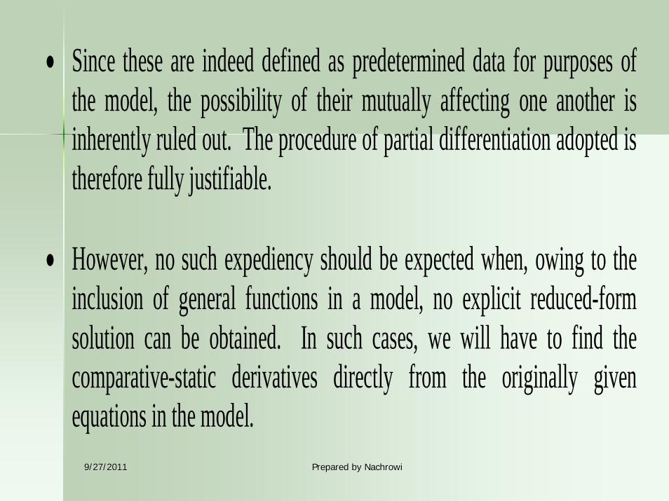
• Since these are indeed defined as predetermined data for purposes ofthe model, the possibility of their mutually affecting one another isinherently ruled out. The procedure of partial differentiation adopted istherefore fully justifiable.

• However, no such expediency should be expected when, owing to the

inclusion of general functions in a model, no explicit reduced-form solution can be obtained. In such cases, we will have to find thecomparative-static derivatives directly from the originally givenequations in the model.


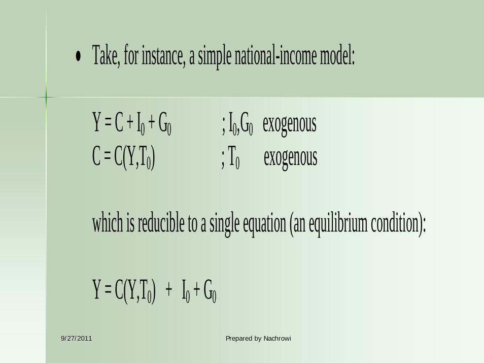
• Take, for instance, a simple national-income model:

Y = C + I0 + G0 ; I0,G0 exogenous C = C(Y,T0) ; T0 exogenous

which is reducible to a single equation (an equilibrium condition): Y = C(Y,T0) + I0 + G0


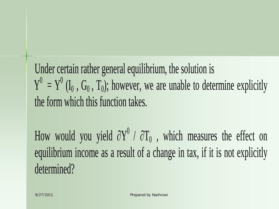
Under certain rather general equilibrium, the solution is Y0 = Y0 (I0 , G0

, T0); however, we are unable to determine explicitlythe form which this function takes. How would you yield ∂Y0 / ∂T0 , which measures the effect onequilibrium income as a result of a change in tax, if it is not explicitlydetermined?


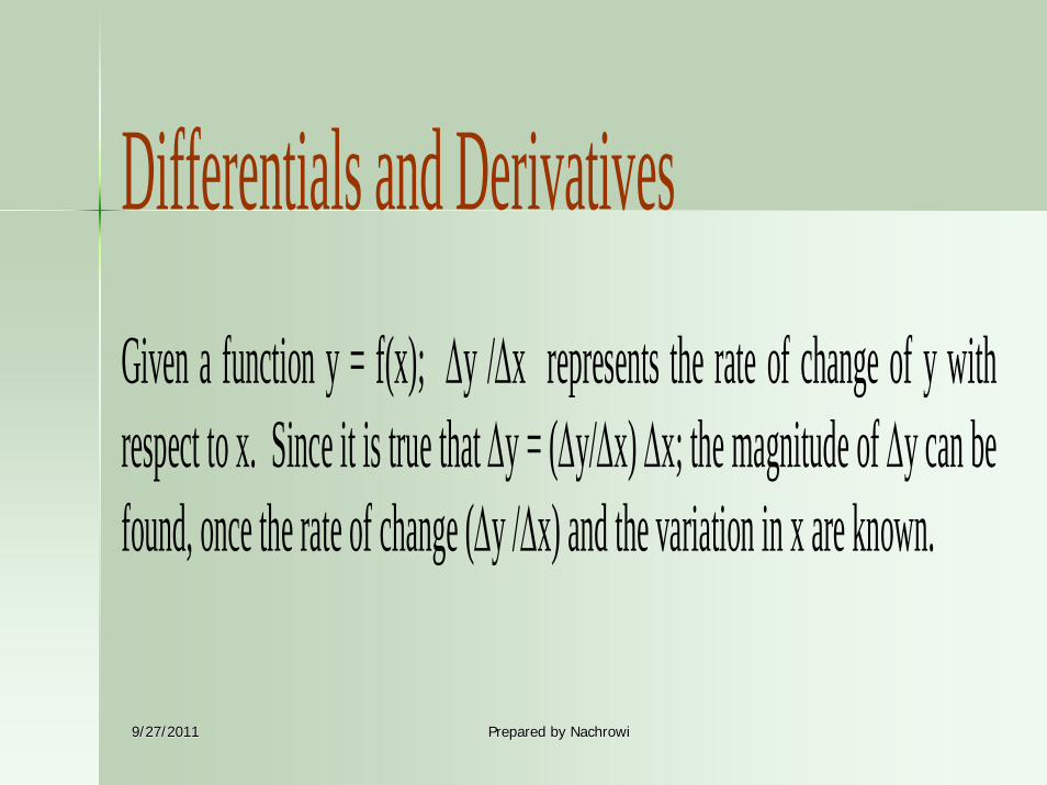
Differentials and Derivatives Given a function y = f(x); Δy /Δx represents the rate of change of y withrespect to x. Since it is true that Δy = (Δy/Δx) Δx; the magnitude of Δy can be found, once the rate of change (Δy /Δx) and the variation in x are known.


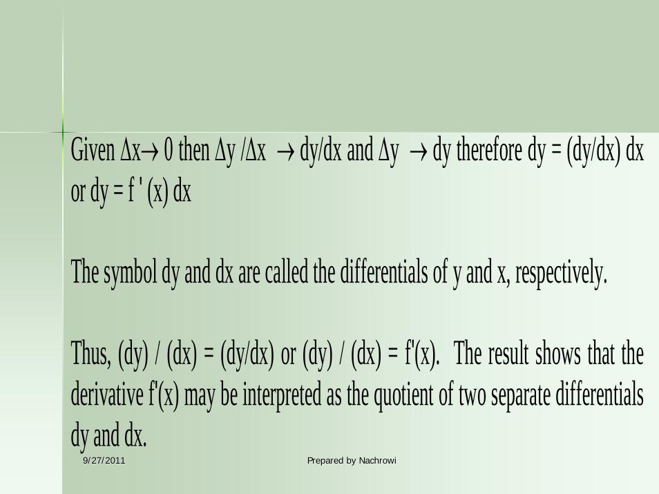
Given Δx→ 0 then Δy /Δx → dy/dx and Δy → dy therefore dy = (dy/dx) dx or dy = f ' (x) dx The symbol dy and dx are called the differentials of y and x, respectively. Thus, (dy) / (dx) = (dy/dx) or (dy) / (dx) = f'(x). The result shows that thederivative f'(x) may be interpreted as the quotient of two separate differentialsdy and dx.


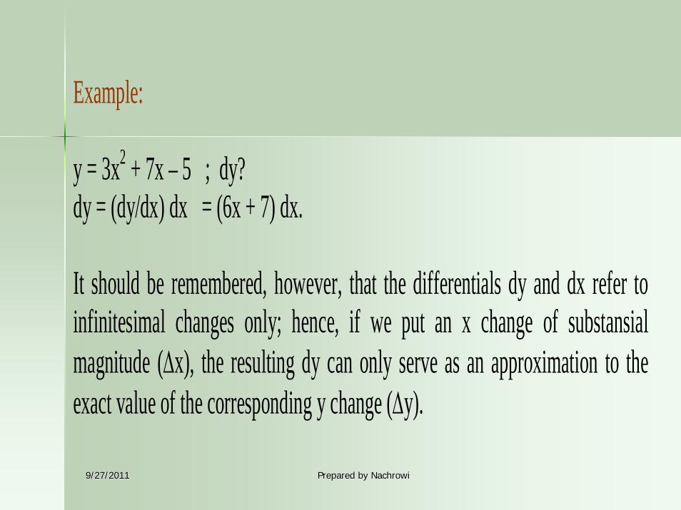
Example: y = 3x2 + 7x – 5 ; dy? dy = (dy/dx) dx = (6x + 7) dx. It should be remembered, however, that the differentials dy and dx refer toinfinitesimal changes only; hence, if we put an x change of substansialmagnitude (Δx), the resulting dy can only serve as an approximation to theexact value of the corresponding y change (Δy).


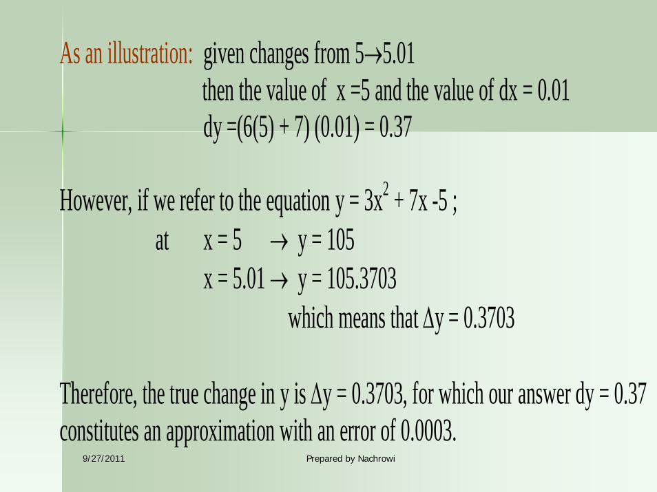
As an illustration: given changes from 5→5.01 then the value of x =5 and the value of dx = 0.01 dy =(6(5) + 7) (0.01) = 0.37 However, if we refer to the equation y = 3x2 + 7x -5 ; at x = 5 → y = 105 x = 5.01 → y = 105.3703 which means that Δy = 0.3703 Therefore, the true change in y is Δy = 0.3703, for which our answer dy = 0.37 constitutes an approximation with an error of 0.0003.


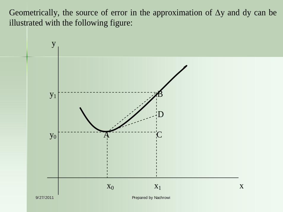
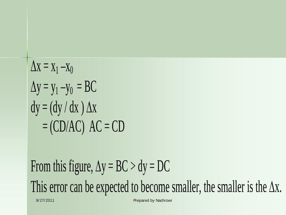
Geometrically, the source of error in the approximation of Δy and dy can beillustrated with the following figure: y y1 B D y0 A C x0 x1 x


Δx = x1 –x0

Δy = y1 –y0 = BC dy = (dy / dx ) Δx = (CD/AC) AC = CD From this figure, Δy = BC > dy = DC This error can be expected to become smaller, the smaller is the Δx.


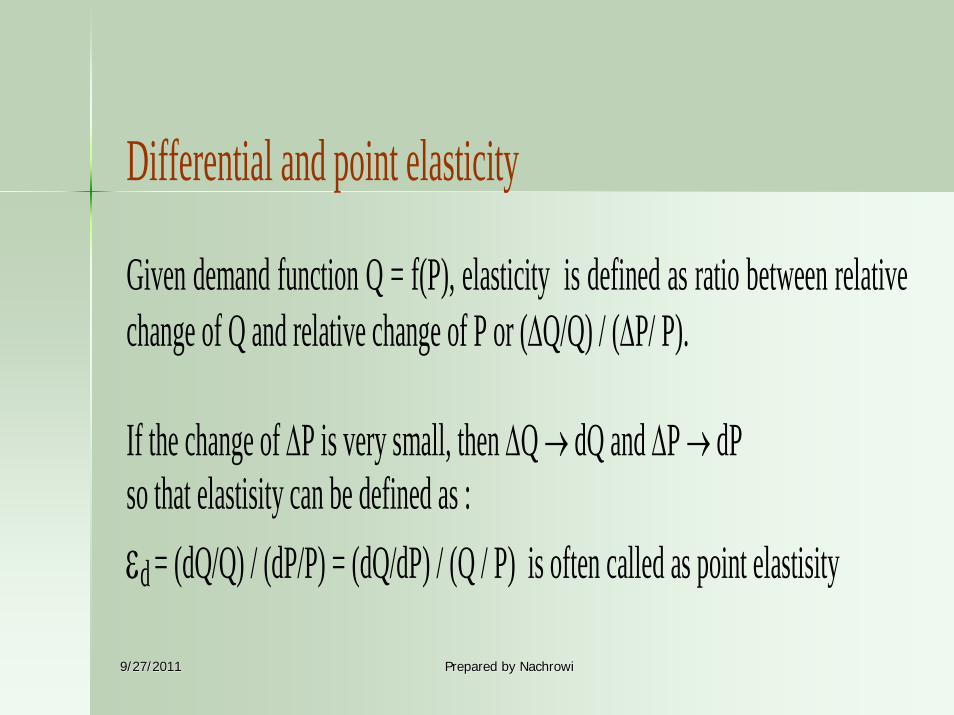
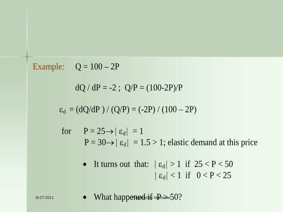
Differential and point elasticity Given demand function Q = f(P), elasticity is defined as ratio between relative change of Q and relative change of P or (ΔQ/Q) / (ΔP/ P). If the change of ΔP is very small, then ΔQ → dQ and ΔP → dP so that elastisity can be defined as : εd = (dQ/Q) / (dP/P) = (dQ/dP) / (Q / P) is often called as point elastisity


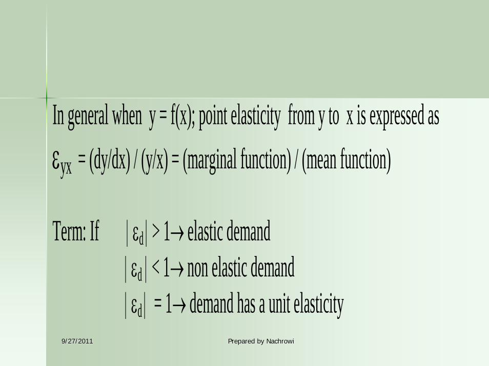
In general when y = f(x); point elasticity from y to x is expressed as εyx = (dy/dx) / (y/x) = (marginal function) / (mean function) Term: If | εd | > 1→ elastic demand | εd | < 1→ non elastic demand | εd | = 1→ demand has a unit elasticity


Example: Q = 100 – 2P dQ / dP = -2 ; Q/P = (100-2P)/P εd = (dQ/dP ) / (Q/P) = (-2P) / (100 – 2P) for P = 25→ | εd | = 1 P = 30→ | εd | = 1.5 > 1; elastic demand at this price

• It turns out that: | εd | > 1 if 25 < P < 50

| εd | < 1 if 0 < P < 25

• What happened if P > 50?


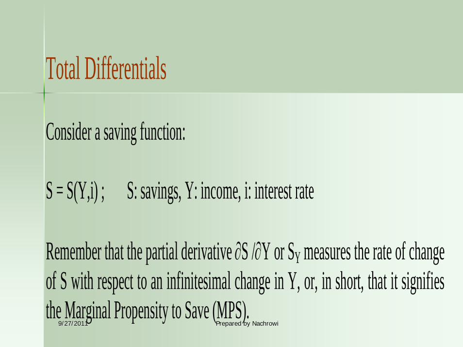
Total Differentials Consider a saving function: S = S(Y,i) ; S: savings, Y: income, i: interest rate Remember that the partial derivative ∂S /∂Y or SY measures the rate of change of S with respect to an infinitesimal change in Y, or, in short, that it signifies the Marginal Propensity to Save (MPS).


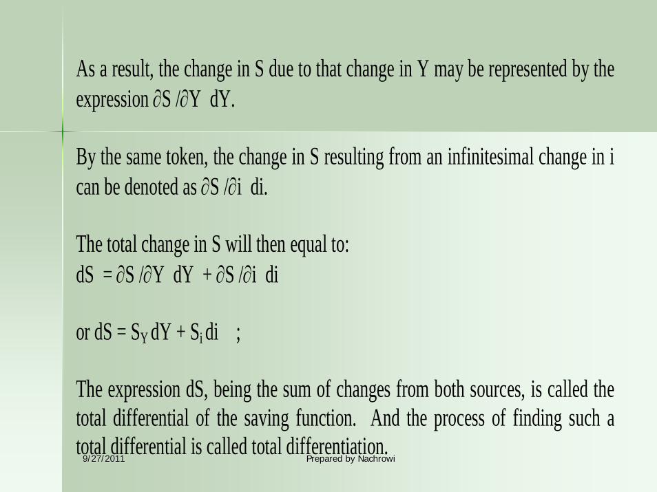
As a result, the change in S due to that change in Y may be represented by theexpression ∂S /∂Y dY. By the same token, the change in S resulting from an infinitesimal change in ican be denoted as ∂S /∂i di. The total change in S will then equal to: dS = ∂S /∂Y dY + ∂S /∂i di or dS = SY dY + Si di ; The expression dS, being the sum of changes from both sources, is called thetotal differential of the saving function. And the process of finding such atotal differential is called total differentiation.


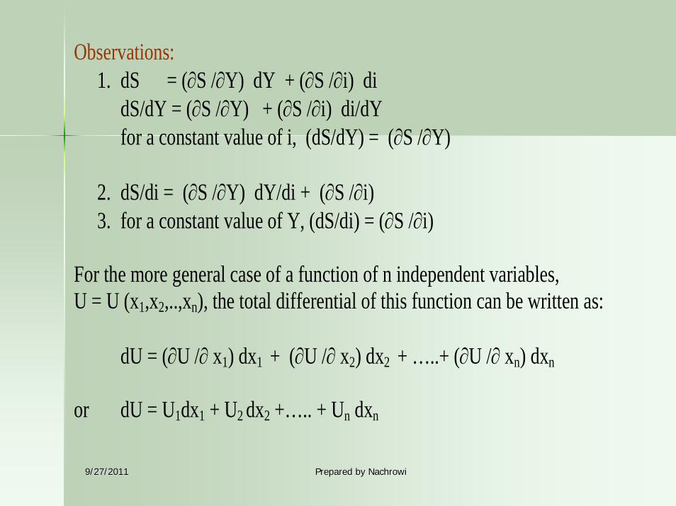
Observations: 1. dS = (∂S /∂Y) dY + (∂S /∂i) di

dS/dY = (∂S /∂Y) + (∂S /∂i) di/dY for a constant value of i, (dS/dY) = (∂S /∂Y)

2. dS/di = (∂S /∂Y) dY/di + (∂S /∂i) 3. for a constant value of Y, (dS/di) = (∂S /∂i)

For the more general case of a function of n independent variables, U = U (x1,x2,..,xn), the total differential of this function can be written as: dU = (∂U /∂ x1) dx1 + (∂U /∂ x2) dx2 + …..+ (∂U /∂ xn) dxn or dU = U1dx1 + U2 dx2 +….. + Un dxn


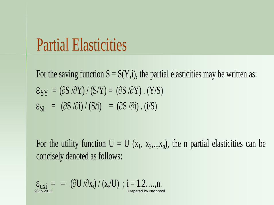
Partial Elasticities For the saving function S = S(Y,i), the partial elasticities may be written as: εSY = (∂S /∂Y) / (S/Y) = (∂S /∂Y) . (Y/S) εSi = (∂S /∂i) / (S/i) = (∂S /∂i) . (i/S) For the utility function U = U (x1, x2,..,xn), the n partial elasticities can be concisely denoted as follows: εuxi = = (∂U /∂xi) / (xi/U) ; i = 1,2….,n.


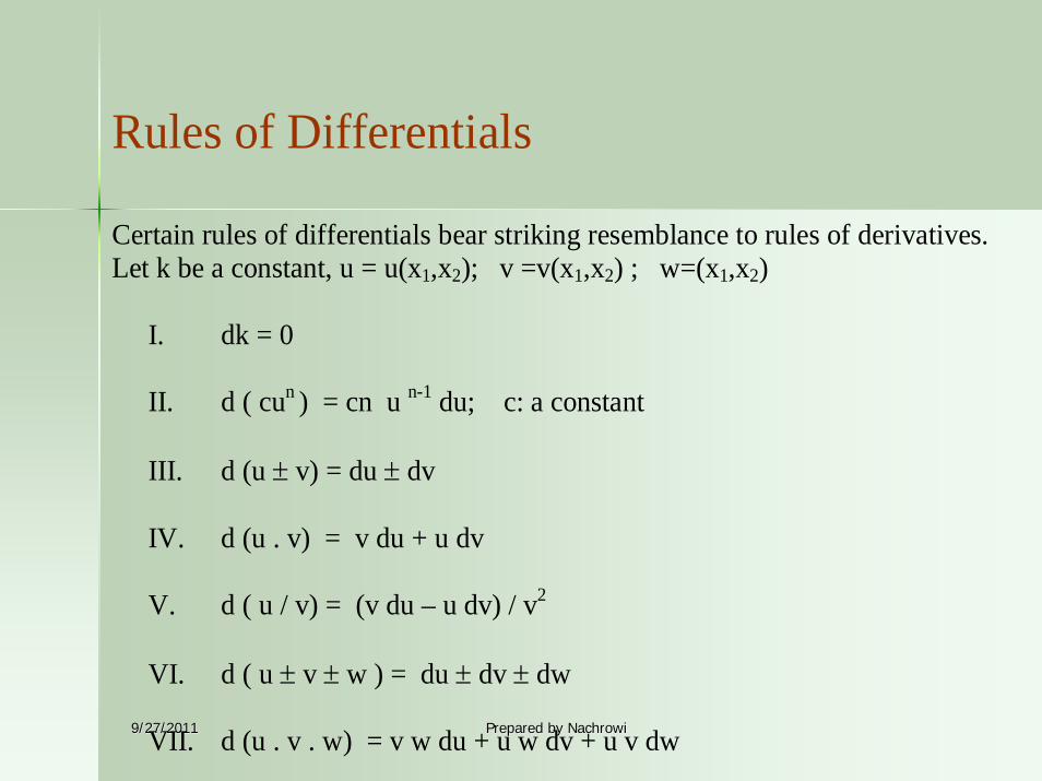
Rules of Differentials Certain rules of differentials bear striking resemblance to rules of derivatives.Let k be a constant, u = u(x1,x2); v =v(x1,x2) ; w=(x1,x2)

I. dk = 0 II. d ( cun ) = cn u n-1 du; c: a constant III. d (u ± v) = du ± dv

IV. d (u . v) = v du + u dv

V. d ( u / v) = (v du – u dv) / v2

VI. d ( u ± v ± w ) = du ± dv ± dw

VII. d (u . v . w) = v w du + u w dv + u v dw


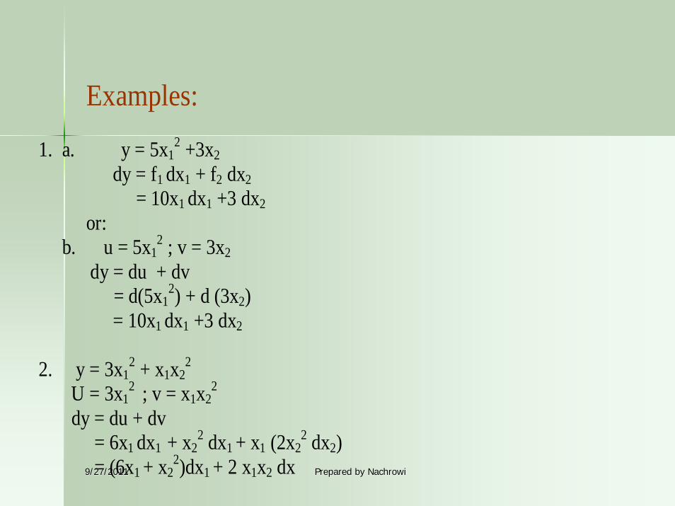
Examples: 1. a. y = 5x1

2 +3x2 dy = f1 dx1 + f2 dx2 = 10x1 dx1 +3 dx2 or: b. u = 5x1

2 ; v = 3x2 dy = du + dv = d(5x1

2) + d (3x2) = 10x1 dx1 +3 dx2 2. y = 3x1

2 + x1x22

U = 3x12 ; v = x1x2

2 dy = du + dv = 6x1 dx1 + x2

2 dx1 + x1 (2x22 dx2)

= (6x1 + x22)dx1 + 2 x1x2 dx


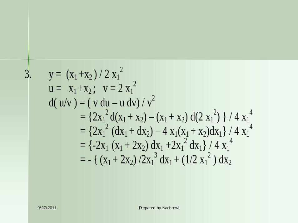
3. y = (x1 +x2 ) / 2 x12

u = x1 +x2 ; v = 2 x12

d( u/v ) = ( v du – u dv) / v2 = {2x1

2 d(x1 + x2) – (x1 + x2) d(2 x12) } / 4 x1

4 = {2x1

2 (dx1 + dx2) – 4 x1(x1 + x2)dx1} / 4 x14

= {-2x1 (x1 + 2x2) dx1 +2x1

2 dx1} / 4 x14

= - { (x1 + 2x2) /2x13 dx1 + (1/2 x1

2 ) dx2


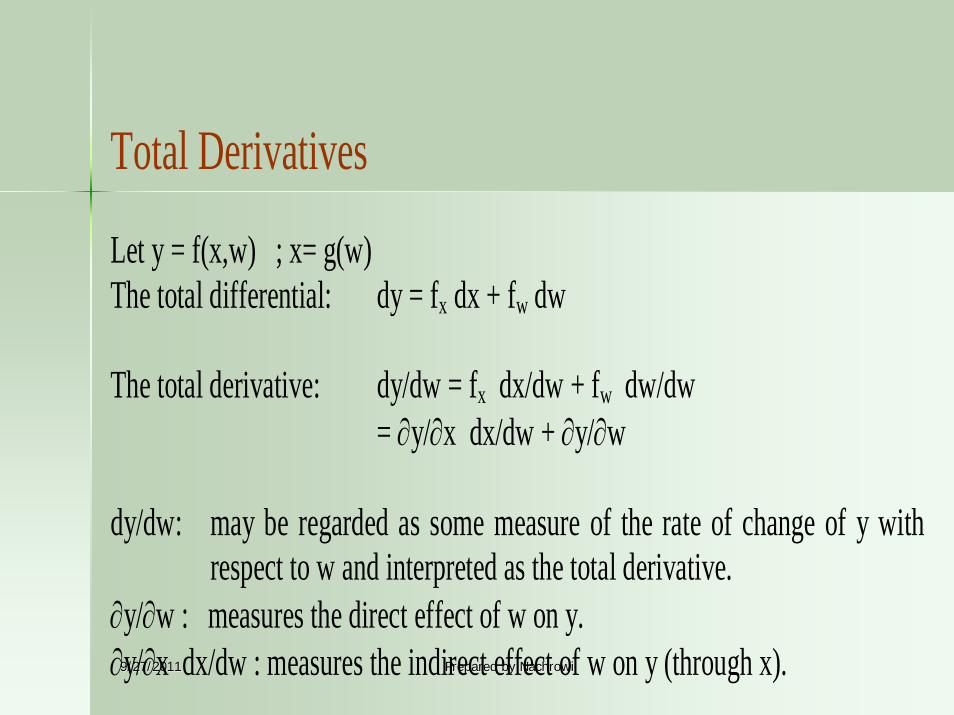
Total Derivatives Let y = f(x,w) ; x= g(w) The total differential: dy = fx dx + fw dw The total derivative: dy/dw = fx dx/dw + fw dw/dw = ∂y/∂x dx/dw + ∂y/∂w dy/dw: may be regarded as some measure of the rate of change of y with

respect to w and interpreted as the total derivative. ∂y/∂w : measures the direct effect of w on y. ∂y/∂x dx/dw : measures the indirect effect of w on y (through x).


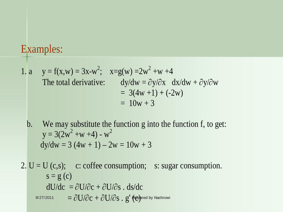
Examples: 1. a y = f(x,w) = 3x-w2; x=g(w) =2w2 +w +4 The total derivative: dy/dw = ∂y/∂x dx/dw + ∂y/∂w = 3(4w +1) + (-2w) = 10w + 3

b. We may substitute the function g into the function f, to get: y = 3(2w2 +w +4) - w2 dy/dw = 3 (4w + 1) – 2w = 10w + 3 2. U = U (c,s); c: coffee consumption; s: sugar consumption. s = g (c) dU/dc = ∂U/∂c + ∂U/∂s . ds/dc = ∂U/∂c + ∂U/∂s . g' (c)


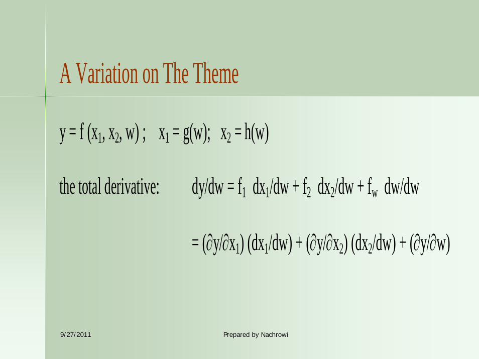
A Variation on The Theme y = f (x1, x2, w) ; x1 = g(w); x2 = h(w) the total derivative: dy/dw = f1 dx1/dw + f2 dx2/dw + fw dw/dw = (∂y/∂x1) (dx1/dw) + (∂y/∂x2) (dx2/dw) + (∂y/∂w)


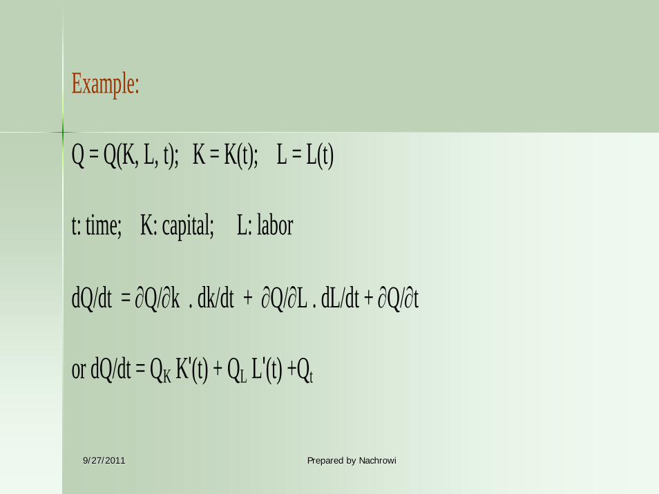
Example: Q = Q(K, L, t); K = K(t); L = L(t) t: time; K: capital; L: labor dQ/dt = ∂Q/∂k . dk/dt + ∂Q/∂L . dL/dt + ∂Q/∂t or dQ/dt = QK K'(t) + QL L'(t) +Qt


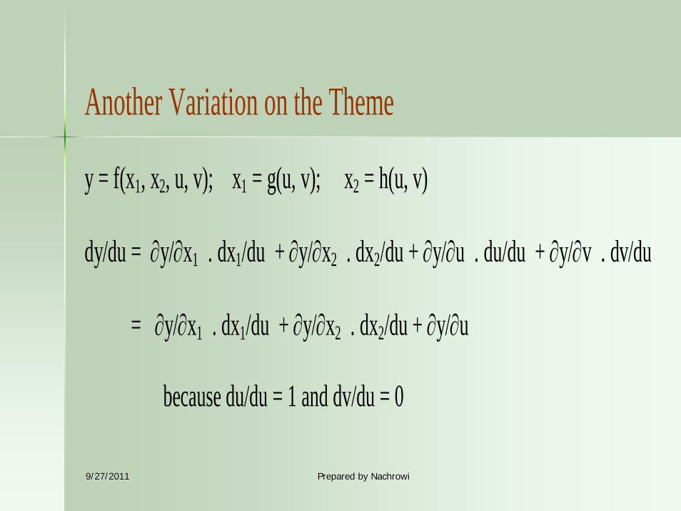
Another Variation on the Theme y = f(x1, x2, u, v); x1 = g(u, v); x2 = h(u, v) dy/du = ∂y/∂x1 . dx1/du + ∂y/∂x2 . dx2/du + ∂y/∂u . du/du + ∂y/∂v . dv/du = ∂y/∂x1 . dx1/du + ∂y/∂x2 . dx2/du + ∂y/∂u because du/du = 1 and dv/du = 0


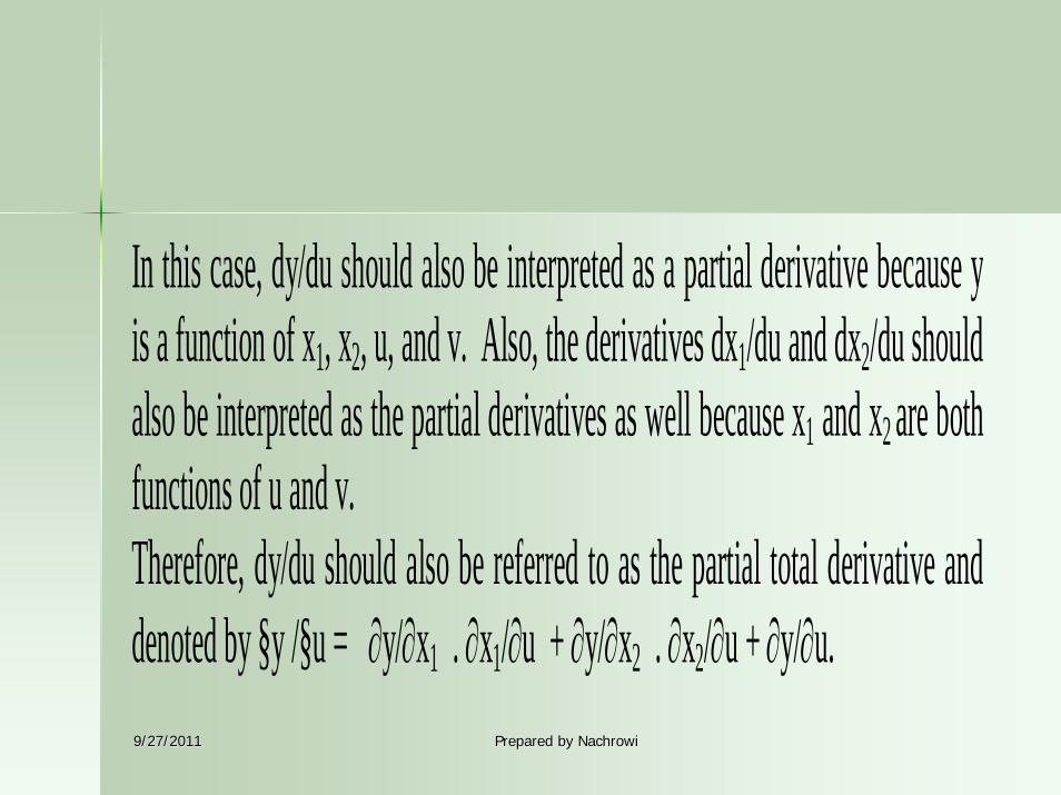
In this case, dy/du should also be interpreted as a partial derivative because yis a function of x1, x2, u, and v. Also, the derivatives dx1/du and dx2/du shouldalso be interpreted as the partial derivatives as well because x1 and x2 are bothfunctions of u and v. Therefore, dy/du should also be referred to as the partial total derivative anddenoted by §y /§u = ∂y/∂x1 . ∂x1/∂u + ∂y/∂x2 . ∂x2/∂u + ∂y/∂u.


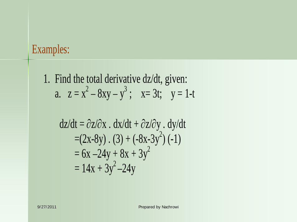
Examples:

1. Find the total derivative dz/dt, given: a. z = x2 – 8xy – y3 ; x= 3t; y = 1-t dz/dt = ∂z/∂x . dx/dt + ∂z/∂y . dy/dt

=(2x-8y) . (3) + (-8x-3y2) (-1) = 6x –24y + 8x + 3y2 = 14x + 3y2 –24y


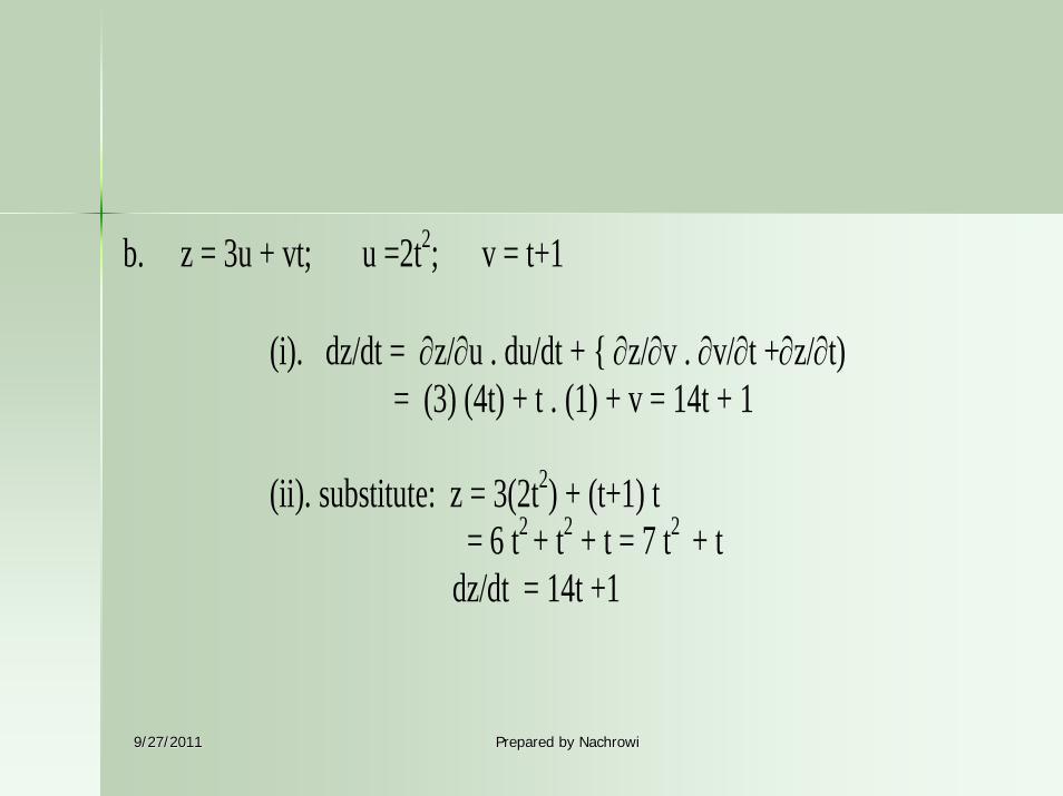
b. z = 3u + vt; u =2t2; v = t+1 (i). dz/dt = ∂z/∂u . du/dt + { ∂z/∂v . ∂v/∂t +∂z/∂t) = (3) (4t) + t . (1) + v = 14t + 1 (ii). substitute: z = 3(2t2) + (t+1) t = 6 t2 + t2 + t = 7 t2 + t dz/dt = 14t +1


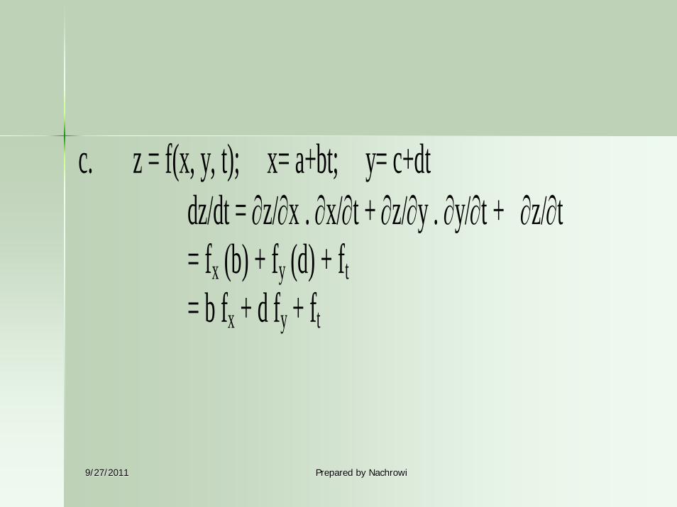
c. z = f(x, y, t); x= a+bt; y= c+dt dz/dt = ∂z/∂x . ∂x/∂t + ∂z/∂y . ∂y/∂t + ∂z/∂t = fx (b) + fy (d) + ft = b fx + d fy + ft


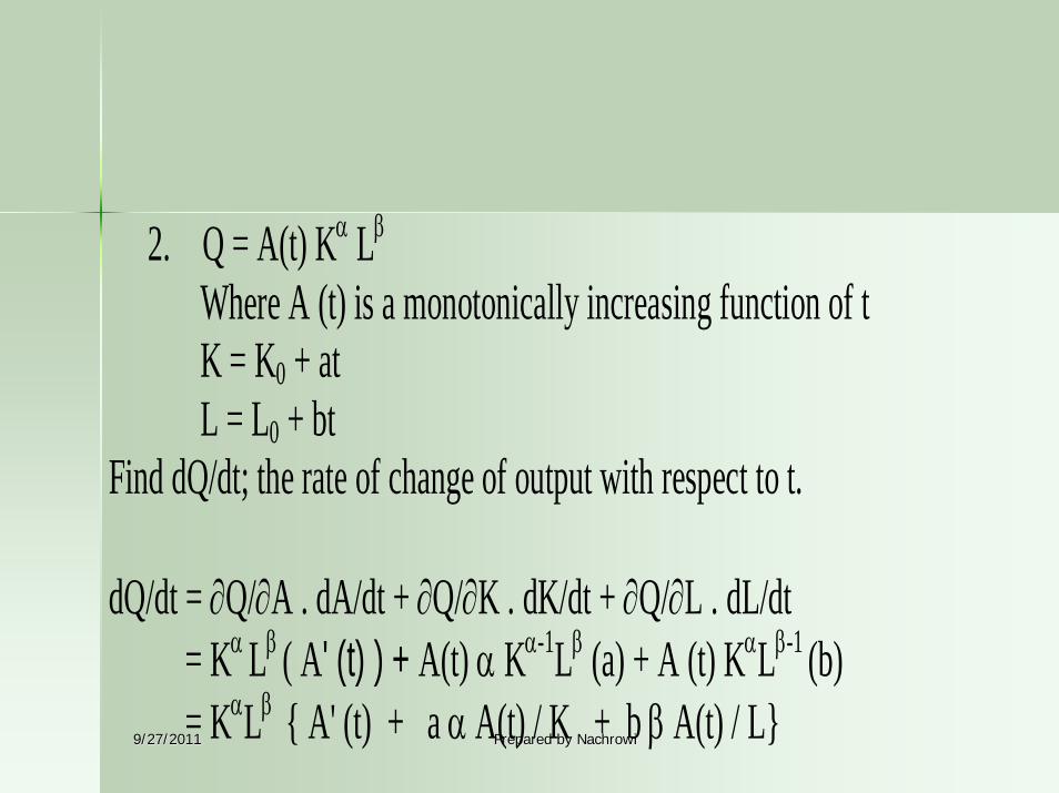
2. Q = A(t) Kα Lβ Where A (t) is a monotonically increasing function of t K = K0 + at L = L0 + bt Find dQ/dt; the rate of change of output with respect to t. dQ/dt = ∂Q/∂A . dA/dt + ∂Q/∂K . dK/dt + ∂Q/∂L . dL/dt = Kα Lβ ( A' (t) ) + A(t) α Kα-1Lβ (a) + A (t) KαLβ-1 (b) = KαLβ { A' (t) + a α A(t) / K + b β A(t) / L}


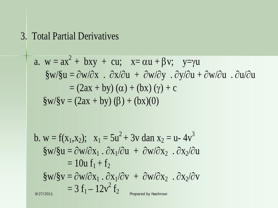
3. Total Partial Derivatives a. w = ax2 + bxy + cu; x= αu + βv; y=γu §w/§u = ∂w/∂x . ∂x/∂u + ∂w/∂y . ∂y/∂u + ∂w/∂u . ∂u/∂u = (2ax + by) (α) + (bx) (γ) + c §w/§v = (2ax + by) (β) + (bx)(0) b. w = f(x1,x2); x1 = 5u2

+ 3v dan x2 = u- 4v3

§w/§u = ∂w/∂x1 . ∂x1/∂u + ∂w/∂x2 . ∂x2/∂u = 10u f1 + f2

§w/§v = ∂w/∂x1 . ∂x1/∂v + ∂w/∂x2 . ∂x2/∂v = 3 f1 – 12v2 f2


The end of The end of the lessonthe lesson

Created by Nachrowi D. Nachrowi.Created by Nachrowi D. Nachrowi.

chapter 8 chiang

Documents