chapter 9 fluids - universiteit...
TRANSCRIPT

Chapter 9
Fluids
9.1 Newtonian Fluids
The equations of motion for an incompressible Newtonian fluid were derivedin the previous chapter. The conclusion was that the constitutive law for thestress is
T = −pI + 2µD, (9.1)
where p is the pressure, D is the rate of deformation tensor given in (8.67),and µ is the dynamic viscosity. The SI unit for µ is the Pascal-second (Pas), and to help provide some perspective on this, the viscosities of some well-known fluids are given in Table 9.1. Not unexpectedly, the viscosity of air issignificantly less than the viscosity of water, which in turn is less viscous thanolive oil. What might seem odd is that there is an entry for peanut butter,which was determined experimentally in Baker et al. [2004]. You might thinkthat a substance like peanut butter behaves more as a solid than a fluid.This is partly due to the length of time it takes peanut butter to flow. It is soslow that it seems to have more of the characteristics of a solid. As it turnsout, peanut butter is not a Newtonian fluid, but this is not due to its slowflow characteristic. It has properties similar to toothpaste and ketchup, twomaterials that are discussed in more depth in the next section.
Fluid Viscosity (Pa s) Density (kg/m3)
Air 1.8× 10⁻⁵ 1.18
Water 0.89× 10⁻³ 0.997× 10³
Mercury 1.5× 10⁻³ 1.3× 10⁴
Olive Oil 0.8× 10⁻¹ 0.92× 10³
Peanut Butter 1.2× 10⁵ 1.02× 10³
Table 9.1 Viscosity and density of various substances at 25 C.
M.H. Holmes, Introduction to the Foundations of Applied Mathematics, 403Texts in Applied Mathematics 56, DOI 10.1007/978-0-387-87765-5 9,c© Springer Science+Business Media, LLC 2009

404 9 Fluids
The question that arose about peanut butter is one of the objectives ofthis chapter, namely how can you determine if a substance can be modeledas a Newtonian fluid? This same question came up in Chapters 6 and 7 whenstudying elasticity and viscoelasticity, and the answer is the same as before.Namely, we will derive solutions to the equations of motion and then comparethem with what is found experimentally. Assuming they agree then we shouldbe able to use the experimental data to determine the viscosity. We will alsouse this approach to investigate various simplifications that can be made inthe Newtonian model. For example, the viscosity of air is so small, it wouldseem that it might be possible to simply assume it is zero. This assumptionproduces what is known as an inviscid fluid, and the resulting mathematicalproblem gives the appearance of being simpler than what is obtained for aviscous fluid. In this chapter a progression of such simplifying assumptions isexamined, with the goal of better understanding fluid motion.
9.2 Steady Flow
One of the more studied problems in fluids involves steady flow. This meansthat the fluid velocity and pressure are independent of time. Assuming thereare no body forces then the equations of motion for a steady incompressiblefluid, coming from (8.77) and (8.78), are
ρ(v · ∇)v = −∇p+ µ∇2v, (9.2)∇ · v = 0. (9.3)
As always, with incompressible motion, it is assumed that ρ is constant.We will solve several fluid problems, and it is always of interest on such
occasions to be able to visualize the flow. One method is to find the pathsof individual fluid particles as the fluid moves, what are known as pathlines.Once the velocity is known, then the pathline x = X(t) that starts out atx = A is found by solving
dXdt
= v(X, t), (9.4)
whereX(0) = A.
As is probably evident, a pathline is just the position function used to definematerial coordinates introduced in Sections 6.2 and 8.2. As demonstrated inExercise 6.3, even for one dimensional motion it is not particularly easy tofind an analytical solution of (9.4). For steady motion, which is what we arecurrently investigating, the problem is a bit easier as the velocity does notdepend explicitly on time. However, for most problems numerical methodsare usually needed to find the solution.

9.2 Steady Flow 405
Figure 9.1 In plane Couette flow the lower plate is stationary, while the top platemoves in the x-direction. Solving this problem shows that the velocity of the fluidvaries linearly between the two plates.
9.2.1 Plane Couette Flow
One of the more basic flows arises when studying the motion of a fluid betweentwo parallel plates. A cross-section of this configuration is shown in Figure9.1. The lower plate, located at y = 0, is fixed, while the upper plate, aty = h, moves with a constant velocity u0 in the x-direction. The associatedboundary conditions are
v = (u0, 0, 0) on y = h, (9.5)v = 0 on y = 0. (9.6)
It is assumed that the upper plate has been moving with this constant velocityfor a long time, so the flow is steady. It is also assumed that the fluid isincompressible, so (9.2), (9.3) apply.
At first glance, given that (9.2) is a nonlinear partial differential equation,finding the velocity and pressure would seem to be an almost impossibletask. However, some useful insights on the properties of the solution can bederived from the boundary conditions and the geometry. In particular, giventhat the upper and lower boundaries are flat plates, and the upper one moveswith a constant velocity in the x-direction, it is not unreasonable to guessthat there is no dependence on, or motion in, the z-direction. In other wordsv = (u, v, 0), where u, v, and p are independent of z. In this case, (9.2), (9.3)reduce to
ρ(u∂x + v∂y)u = −∂xp+ µ∇2u,
ρ(u∂x + v∂y)v = −∂yp+ µ∇2v,
∂xu+ ∂yv = 0.
This is still a formidable problem, so we need another insight into the formof the solution. Given that the upper plate is sliding in the x-direction, it isnot unreasonable to expect that there is no flow in the y-direction. In thiscase, v = 0 and the above system reduces to

406 9 Fluids
ρu∂xu = −∂xp+ µ∂2yu,
0 = −∂yp,
∂xu = 0.
From the last two equations we have that p = p(x) and u = u(y). In this case,the first equation reduces to p′(x) = µu′′(y). The only way for a function ofx to equal a function of y is that both functions are constants. Consequently,p′(x) constant means p(x) = p0 + xp1, where p0 and p1 are constants. It isassumed that the pressure remains bounded, and so p1 = 0. With this, thesolution of µu′′(y) = p′(x) is u = ay + b. Imposing the boundary conditionsu(0) = 0 and u(h) = u0, it follows that u = u0y/h.
The solution of the plane Couette flow problem is, therefore,
v = (γy, 0, 0), (9.7)
where p = p0 is constant, andγ =
u0
h(9.8)
is known as the shear rate. This shows that the fluid velocity in the x-directionincreases linearly between the two plates, from zero to u0. This dependenceis illustrated in Figure 9.2. Also, the resulting fluid stress tensor (9.9) is
T = −p0I + µ
0
u0
h0
u0
h0 0
0 0 0
. (9.9)
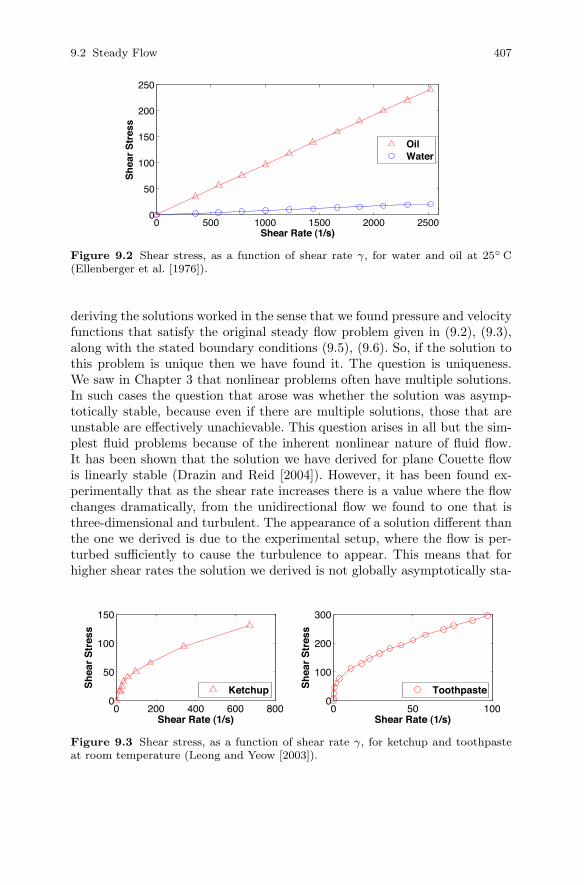
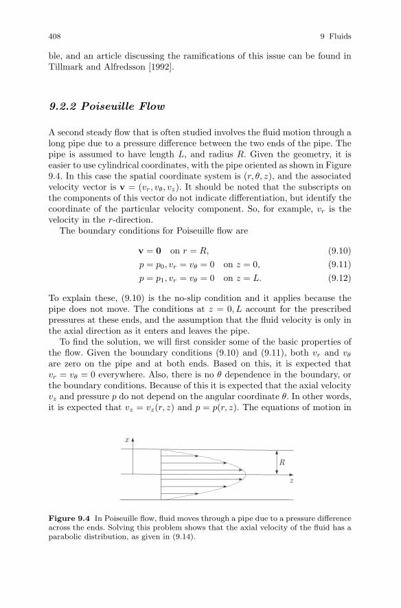
The above solution gives us something we sorely need, and that is a methodfor checking on the assumption that a fluid is Newtonian. The solution showsthat for a Newtonian fluid the shear stress is T12 = µu0/h. Therefore, theshear stress depends linearly on the shear rate γ = u0/h, with the slope ofthe curve equal to the viscosity. This is the basis for one of the more impor-tant experiments in fluid dynamics, where the shear stress is measured as afunction of the shear rate. Results from such tests are shown in Figures 9.2and 9.3, for fluids most people have experience with. Based on the linearityof the data in Figure 9.2, the assumption that water and oil are Newtonian isreasonable. For the same reason, from Figure 9.3, ketchup and toothpaste arenot Newtonian, or only Newtonian for very small shear rates. They are exam-ples of what are called nonlinear power-law fluids, where T12 = αγβ . Basedon the data in Figure 9.3, for ketchup, β = 0.55, where as for toothpaste,β = 0.44. Some of the implications of such a constitutive law are investigatedin Exercise 9.7.
Before moving on to another topic, a comment needs to be made aboutour solution of the plane Couette flow problem. The assumptions we made in
9.2 Steady Flow 407
0 500 1000 1500 2000 25000
50
100
150
200
250
Shear Rate (1/s)
Shea
r Stre
ss
Oil Water
Figure 9.2 Shear stress, as a function of shear rate γ, for water and oil at 25 C(Ellenberger et al. [1976]).
deriving the solutions worked in the sense that we found pressure and velocityfunctions that satisfy the original steady flow problem given in (9.2), (9.3),along with the stated boundary conditions (9.5), (9.6). So, if the solution tothis problem is unique then we have found it. The question is uniqueness.We saw in Chapter 3 that nonlinear problems often have multiple solutions.In such cases the question that arose was whether the solution was asymp-totically stable, because even if there are multiple solutions, those that areunstable are effectively unachievable. This question arises in all but the sim-plest fluid problems because of the inherent nonlinear nature of fluid flow.It has been shown that the solution we have derived for plane Couette flowis linearly stable (Drazin and Reid [2004]). However, it has been found ex-perimentally that as the shear rate increases there is a value where the flowchanges dramatically, from the unidirectional flow we found to one that isthree-dimensional and turbulent. The appearance of a solution different thanthe one we derived is due to the experimental setup, where the flow is per-turbed sufficiently to cause the turbulence to appear. This means that forhigher shear rates the solution we derived is not globally asymptotically sta-
0 200 400 600 8000
50
100
150
Shear Rate (1/s)
Shea
r Stre
ss
Ketchup
0 50 1000
100
200
300
Shear Rate (1/s)
Shea
r Stre
ss
Toothpaste
Figure 9.3 Shear stress, as a function of shear rate γ, for ketchup and toothpasteat room temperature (Leong and Yeow [2003]).
408 9 Fluids
ble, and an article discussing the ramifications of this issue can be found inTillmark and Alfredsson [1992].
9.2.2 Poiseuille Flow
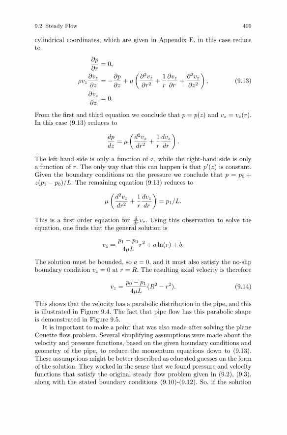
A second steady flow that is often studied involves the fluid motion through along pipe due to a pressure difference between the two ends of the pipe. Thepipe is assumed to have length L, and radius R. Given the geometry, it iseasier to use cylindrical coordinates, with the pipe oriented as shown in Figure9.4. In this case the spatial coordinate system is (r, θ, z), and the associatedvelocity vector is v = (vr, vθ, vz). It should be noted that the subscripts onthe components of this vector do not indicate differentiation, but identify thecoordinate of the particular velocity component. So, for example, vr is thevelocity in the r-direction.
The boundary conditions for Poiseuille flow are
v = 0 on r = R, (9.10)p = p0, vr = vθ = 0 on z = 0, (9.11)p = p1, vr = vθ = 0 on z = L. (9.12)
To explain these, (9.10) is the no-slip condition and it applies because thepipe does not move. The conditions at z = 0, L account for the prescribedpressures at these ends, and the assumption that the fluid velocity is only inthe axial direction as it enters and leaves the pipe.
To find the solution, we will first consider some of the basic properties ofthe flow. Given the boundary conditions (9.10) and (9.11), both vr and vθ
are zero on the pipe and at both ends. Based on this, it is expected thatvr = vθ = 0 everywhere. Also, there is no θ dependence in the boundary, orthe boundary conditions. Because of this it is expected that the axial velocityvz and pressure p do not depend on the angular coordinate θ. In other words,it is expected that vz = vz(r, z) and p = p(r, z). The equations of motion in
Figure 9.4 In Poiseuille flow, fluid moves through a pipe due to a pressure differenceacross the ends. Solving this problem shows that the axial velocity of the fluid has aparabolic distribution, as given in (9.14).
9.2 Steady Flow 409
cylindrical coordinates, which are given in Appendix E, in this case reduceto
∂p
∂r= 0,
ρvz∂vz
∂z= −∂p
∂z+ µ
(∂2vz
∂r2+
1r
∂vz
∂r+∂2vz
∂z2
), (9.13)
∂vz
∂z= 0.
From the first and third equation we conclude that p = p(z) and vz = vz(r).In this case (9.13) reduces to
dp
dz= µ
(d2vz
dr2+
1r
dvz
dr
).
The left hand side is only a function of z, while the right-hand side is onlya function of r. The only way that this can happen is that p′(z) is constant.Given the boundary conditions on the pressure we conclude that p = p0 +z(p1 − p0)/L. The remaining equation (9.13) reduces to
µ
(d2vz
dr2+
1r
dvz
dr
)= p1/L.
This is a first order equation for ddrvz. Using this observation to solve the
equation, one finds that the general solution is
vz =p1 − p0
4µLr2 + a ln(r) + b.
The solution must be bounded, so a = 0, and it must also satisfy the no-slipboundary condition vz = 0 at r = R. The resulting axial velocity is therefore
vz =p0 − p1
4µL(R2 − r2). (9.14)
This shows that the velocity has a parabolic distribution in the pipe, and thisis illustrated in Figure 9.4. The fact that pipe flow has this parabolic shapeis demonstrated in Figure 9.5.
It is important to make a point that was also made after solving the planeCouette flow problem. Several simplifying assumptions were made about thevelocity and pressure functions, based on the given boundary conditions andgeometry of the pipe, to reduce the momentum equations down to (9.13).These assumptions might be better described as educated guesses on the formof the solution. They worked in the sense that we found pressure and velocityfunctions that satisfy the original steady flow problem given in (9.2), (9.3),along with the stated boundary conditions (9.10)-(9.12). So, if the solution

410 9 Fluids
t = 0
t = 5
t = 10
Figure 9.5 Two fluids flowing, from left to right, in a clear pipe (Kunkle [2008]). Att = 0 the darker fluid is located at the left end. At t = 10 sec the darker fluid showsthe parabolic shape predicted by the solution given in (9.14).
to this problem is unique then we have found it. Moreover, an experimentaldemonstration that the solution has the predicted parabolic profile is shownin Figure 9.5.
As it turns out, experiments show that non-parabolic flow can be obtainedin pipe flow. As with the plane Couette problem, for large enough perturba-tions in the flow, it is found that at high velocities the flow in the pipe canbe three-dimensional and turbulent. This does not mean our solution is inquestion, it just means that it is not globally asymptotically stable at highflow rates. A great deal of effort has been invested into understanding theproperties of flow in a pipe, and a recent review of this work can be found inEckhardt et al. [2007].

9.3 Vorticity 411
9.3 Vorticity
If you float on an inner tube on a river you notice that not only do you movedownstream, the moving water also causes you to spin. It is the rotationalcomponent of the motion that we are now interested in exploring. The firststep is to derive a variable that can be used to measure the rotation, at leastlocally.
To explain how this is done, consider three fluid particles located on thecoordinate axis, at t = 0, as shown in Figure 9.6. For simplicity the flow isassumed to be two-dimensional, and the positions of the three particles att = ∆t are also shown in the figure. The velocity, at t = 0, of the particlelocated at the origin is v0 = (u0, v0), where u0 = u(0, 0) and v0 = v(0, 0).The initial velocity of the particle located at x = ∆x is v1 = (u1, v1), whereu1 = u(∆x, 0) and v1 = v(∆x, 0). We are interested in the case of when ∆xand ∆t are small. In this case, Taylor’s theorem gives us
u1 = u(∆x, 0)= u(0, 0) +∆xux(0, 0) + · · ·= u0 +∆xux + · · · .
Similarly, v1 = v0 +∆xvx + · · · . With this, v1 ≈ v0 +∆x(ux, vx). Now, att = ∆t the particle that started at the origin is located at approximately∆tv0, and the one that started at x = ∆x is at approximately ∆tv1 ≈∆t(v0 +∆x(ux, vx)). With this
tan(θ1) ≈∆t(v0 +∆xvx)−∆tv0
∆x+∆t(u0 +∆xux)−∆tu0
=∆tvx
1 +∆tux
≈ ∆tvx.
Figure 9.6 Three nearby fluid particles used to introduce the concept of vorticity.Their motion from t = 0 to t = ∆t, causes both a translation and relative rotation intheir configuration.

412 9 Fluids
Given that the angle is small, so tan(θ1) ≈ θ1, we have that θ1 ≈ ∆t vx.Carrying out a similar analysis using the particle that started at y = ∆y onefinds that θ2 ≈ −∆tuy. The average angular velocity around the z-axis istherefore (θ1 +θ2)/(2∆t) ≈ 1
2 (vx−uy). Similar expressions can be derived forthe rotation around the other two axes. This is the motivation for introducingthe vorticity ω, which is defined as
ω = ∇× v
=(∂w
∂y− ∂v
∂z
)i +(∂u
∂z− ∂w
∂x
)j +(∂v
∂x− ∂u
∂y
)k, (9.15)
where v = (u, v, w). Consequently, ω is twice the average angular velocityin the three coordinate planes. This also helps explain why W in (8.68) isknown as the vorticity tensor.
Example: Plane Couette Flow
As shown in Figure 9.1, the fluid particles in Couette flow move in straightlines, and, consequently, appear to have no rotational component. However,using the solution (9.7) in (9.15), one obtains ω = (0, 0,−γ). In other words,the vorticity is nonzero. To explain this, plane Couette flow can be thoughtof using traffic flow on a multilane road, where the fluid particles are the cars.This is shown in Figure 9.7. The slowest lane is at y = 0, and the fastest laneis at y = h. Given a line of cars that start out at x = 0, after a short time theywill have a linear distribution as shown in Figure 9.7. A driver in one of middlelanes will see the car on the left a bit farther ahead, and the one on the righta bit farther behind. Hence, from the driver’s perspective there has been arotation in the orientation, the rotation being in the clockwise direction. Thisgives rise to a negative angular velocity, and this is why the z-component ofthe vorticity is negative for this flow. This example also shows that nonzerovorticity does not necessarily mean that the fluid particles themselves arerotating. The definition of vorticity assumes nothing about how the fluidparticles interact, it only measures their respective orientations as they flowpast each other.
9.3.1 Vortex Motion
A vortex is a circular flow around a center, and is similar to what is seenin a tornado, hurricane, and in the swirling flow through a drain. To studysuch motions, it is often convenient to use cylindrical coordinates, and theequations of motion in this coordinate system are given in Appendix E.The coordinates in this system are (r, θ, z), with corresponding velocityv = (vr, vθ, vz). Assuming the center of the vortex is the z-axis then to have

9.3 Vorticity 413
circular motion around the z-axis we assume that vr = vz = 0. This meansthere is no motion in either the z- or r-direction, and so the fluid particlesmove on circles centered on the z-axis. Making the additional assumptionthat vθ = vθ(r, t) then the equations of motion reduce to
∂vθ
∂t= ν
∂
∂r
(1r
∂(rvθ)∂r
), (9.16)
∂p
∂r=ρ
rv2
θ . (9.17)
This assumes the fluid is incompressible, and that there are no body forces.The vorticity for this flow is
ω =(
0, 0,1r
∂(rvθ)∂r
). (9.18)
The momentum equation (9.16) is an old friend because it is the radiallysymmetric diffusion equation given in (4.78). In this case, the kinematic vis-cosity is the diffusion coefficient. The point source solution given in (4.81)gives rise to what is known as the Taylor vortex. The analysis of this vortexis carried out in Exercise 9.10, while we will investigate a related vortex inthe following example.
Example: Oseen-Lamb Vortex
In this flow vr = vz = 0, and
vθ =α
r
(1− exp
(−r2
β2 + 4νt
)). (9.19)
It is not hard to show that this function satisfies (9.16), and is therefore anexact solution of the incompressible fluid equations. The pressure is found byintegrating (9.17), and the vorticity is calculated using (9.18). One finds that
Figure 9.7 Multilane traffic flow analogy used to explain vorticity in plane Couetteflow.

414 9 Fluids
Figure 9.8 The rotational motionof a hurricane is an example of vortextype motion, with the eye containingthe central axis.
ω =(
0, 0,2α
β2 + 4νtexp(
−r2
β2 + 4νt
)). (9.20)
The velocity (9.19) is shown in Figure 9.9 at different time points, for α =β = 4ν = 1. This shows that when the vortex starts out, it is confined to theregion near r = 0. As time passes the vortex slows down, with the maximumvelocity moving outward from the center and decreasing in the process. Thisis due entirely to the viscosity of the fluid, and the result is that in the limitof t→∞, the vortex disappears. Also note that when this vortex starts out,there is a region near r = 0 where there is little motion, which is reminiscentof the eye of the hurricane shown in Figure 9.8.
9.4 Irrotational Flow
One of the ideas underlying the introduction of vorticity is that the mo-tion of a fluid can be split into two components, a rotational part and anon-rotational part. How this can be done is obtained from the HelmholtzRepresentation Theorem, and this will be presented shortly. In preparationfor this we introduce the concept of an irrotational flow.
0 1 2 3 4 5 60
0.4
0.8
r−axis
v−axis
t = 0 t = 2 t = 8
Figure 9.9 Circumferential velocity (9.19) for a Oseen-Lamb vortex.

9.4 Irrotational Flow 415
Definition 9.1. A fluid for which the vorticity is identically zero is said tobe irrotational. The flow is rotational if the vorticity is nonzero anywhere inthe flow.
One might guess that a flow which moves in a straight line is irrotational, butthe plane Couette flow example shows that statement is incorrect. It is alsoincorrect to assume that if the flow is a vortex then it must be rotational.The next example explains why.
Example: Line Vortex
In the special case of when vr = vz = 0, and vθ = vθ(r, t), then the vortic-ity is given in (9.18). This will be zero if rvθ is constant. Consequently, anirrotational flow is achieved by taking
vθ =α
r, (9.21)
where α is a constant. The flow in this case is circular motion around thez-axis, just as it is for the Oseen-Lamb vortex shown in Figure 9.9. This iscalled a line vortex, and it produces irrotational flow.
As the above example clearly demonstrates, rotational motion around theorigin does not necessarily mean that the vorticity is nonzero. The reasonthis is confusing is that vorticity is a local property of the flow, and it isdetermined by the relative movement of nearby fluid particles. This is notnecessarily the same as what is happening to the flow on the macroscopiclevel. This is why the conclusion coming from the line vortex example, thatthis particular rotational flow around the origin is irrotational, is not self-contradictory.
One of the difficulties with assuming a flow is irrotational is that it is astatement about the absence of a property, namely no vorticity. The questionarises whether it might be possible to characterize the solutions of the Navier-Stokes equation that are irrotational. To answer this, we will make use of thefollowing result, which is known as the Helmholtz Representation Theorem.
Theorem 9.1. Assume q(x) is a smooth function of x in a domain D. Inthis case, there exists a scalar function φ(x) and a vector function g(x) sothat for x ∈ D,
q(x) = ∇φ+∇× g, (9.22)
where ∇ · g = 0. The function φ is called the scalar potential, and g is thevector potential, for q.
The proof of this theorem involves two vector identities and a result frompartial differential equations. The first identity is that, given any smoothvector function h(x),

416 9 Fluids
∇2h = ∇(∇ · h)−∇× (∇× h).
The right hand side of this equation resembles the result in (9.22), whereφ = ∇ · h and g = −∇ × h. What is needed is to find h so that q = ∇2h.This is where the result from partial differential equations comes in. Solving∇2h = q for h is known as Poisson’s equation, and a particular solution is(Weinberger [1995])
h(x) = − 14π
∫∫∫D
q(s)||x− s||
dVs, (9.23)
where the subscript s indicates integration with respect to s. With this choicefor h we have derived an expression of the form given in (9.22). The only thingleft to show is that ∇·g = 0. This follows because g = −∇×h and the vectoridentity that states, given any smooth vector function h(x), ∇ · (∇×h) = 0.
The above proof relied on the solution of Poisson’s equation, and thisrequires certain conditions to be satisfied. If the closure of D is a boundedregular region, then the stated assumption that q is smooth is sufficient.Specifically, what this means is that∇×q and∇·q are continuous functions. IfD is not bounded then the integral requires an additional condition, which isthat q goes to zero faster than ||x||−2 as ||x|| → ∞. It is, however, possible tomodify the proof so this latter condition is not needed. The details concerningthe extension to unbounded domains can be found in Gregory [1996].
Another comment concerning the proof is that it is constructive in thesense that it provides formulas for the potential functions. To explore someof the consequences of this, suppose for the moment that D = R3. Given thatφ = ∇ · h, then from (9.23) the scalar potential function can be written as
φ = − 14π∇ ·∫∫∫
q(s)||x− s||
dVs
= − 14π
∫∫∫q · ∇x
1||x− s||
dVs
= − 14π
∫∫∫q · ∇s
1||x− s||
dVs
= − 14π
∫∫∫∇s ·
q||x− s||
− ∇s · q||x− s||
dVs
=14π
∫∫∫∇s · q||x− s||
dVs.
Carrying out a similar calculation for g one finds that the vector potentialcan be written as
g = − 14π
∫∫∫∇s × q||x− s||
dVs. (9.24)

9.4 Irrotational Flow 417
It should be remembered that this is for D = R3, so any contribution fromthe boundary of the domain is not accounted for in this formula.
9.4.1 Potential Flow
We are interested in irrotational fluid motion, and what can be learned usingthe Helmholtz Representation Theorem. Taking q to be the fluid velocitythen ∇×q = ω. For an irrotational flow, so ω = 0, the conclusion we derivefrom (9.22) and (9.24) is that the velocity has the form
v = ∇φ. (9.25)
Any flow in which the velocity can be written in this way is called potentialflow. To investigate the consequences of this, we will assume that the fluid isincompressible and there are no body forces. The continuity equation∇·v = 0in this case reduces to
∇2φ = 0. (9.26)
This means that the velocity can be found by simply solving Laplace’s equa-tion, and this is one of the reasons why potential flow is a centerpiece in mostfluid dynamics textbooks. It is important to point out here that nothing hasbeen said about the boundary conditions. These have major repercussionsfor potential flow, and this will be discussed in more detail shortly.
The pressure p for potential flow is determined by solving the momentumequations. In the x-direction, as given in (8.77), we have that
ρ
(∂2φ
∂x∂t+∂φ
∂x
∂2φ
∂x2+∂φ
∂y
∂2φ
∂x∂y+∂φ
∂z
∂2φ
∂x∂z
)= −∂p
∂x+ µ∇2 ∂φ
∂x. (9.27)
Given (9.26), then the viscous stress term µ∇2∂xφ in the above equation iszero. In other words, for irrotational flow the viscosity does not contributeto the momentum equation. With this, it is possible to rewrite (9.27) in theform
∂
∂x
[∂φ
∂t+
12
(∂φ
∂x
)2
+12
(∂φ
∂y
)2
+12
(∂φ
∂z
)2
+1ρp
]= 0.
Not too surprisingly, the y and z momentum equations show that the yand z derivatives of the above quantity in the square brackets are zero. Theconclusion is that
∂φ
∂t+
12
(∂φ
∂x
)2
+12
(∂φ
∂y
)2
+12
(∂φ
∂z
)2
+1ρp
is only a function of time. In other words,

418 9 Fluids
p = p0(t)− ρ
[∂φ
∂t+
12
(∂φ
∂x
)2
+12
(∂φ
∂y
)2
+12
(∂φ
∂z
)2], (9.28)
or equivalently
p = p0(t)− ρ
(∂φ
∂t+
12∇φ · ∇φ
). (9.29)
This is known as Bernoulli’s theorem for irrotational flow. Once Laplace’sequation is solved to find the potential function, (9.25) is used to find thevelocity and (9.29) is used to find the pressure.
Example: Line Vortex (cont’d)
Using cylindrical coordinates, then v = (vr, vθ, vz), and
∇φ =(∂φ
∂r,1r
∂φ
∂θ,∂φ
∂z
). (9.30)
To obtain vr = vz = 0 it is required that φ = φ(θ, t). To have (9.21) hold itis required that ∂φ
∂θ = α. Therefore, the scalar potential function for the linevortex is φ = αθ. The pressure, obtained from (9.29), is p = p0− 1
2ρα2/r2.
One question that has not been addressed is, how realistic is it to assumea flow is irrotational? In applications, in addition to the equations of mo-tion, there are boundary and initial conditions, and these were convenientlyignored when deriving (9.24). The fact is that they can easily ruin the assump-tion of irrotationality. To explain why, consider the no-slip condition (8.7).This prescribes all three components of the velocity vector on the boundary.The equation to solve for an irrotational flow is Laplace’s equation (9.26),from which the velocities are determined using (9.25). Mathematically, forLaplace’s equation, one can only impose one condition on the boundary, and
Figure 9.10 The motion of theairflow around a plane generatesvorticity into the flow (Morris[2006]). This is evident in the mo-tion of the clouds behind the planein the photograph.

9.5 Ideal Fluid 419
not three as required from the no-slip condition. The usual choice is to havethe solution satisfy the impermeability condition (8.79). Therefore, if the flowis to be irrotational, the other two boundary conditions making up the no-slip condition would have to be selected to be consistent with the resultingsolution of Laplace’s equation. What this means is that irrotational flow in aviscous fluid is possible, but the boundary conditions have to be just right. Anexample is the line vortex above, where there are no boundaries, and henceno difficulties trying to satisfy the no-slip condition. Physically, what hap-pens in most fluid problems is that the boundaries generate vorticity, whichthen spreads into the flow and causes it to be rotational. An example of thisis shown in Figure 9.10. One way to avoid this from happening, in additionto adjusting the boundary conditions, is to assume the fluid viscosity is zero.This produces what is known as an inviscid fluid, and this is the subject ofthe next section.
Because of the complications of the no-slip condition, most textbooks as-sociate potential flow with an inviscid fluid. In fact, to overcome this asso-ciation, in the research literature the above discussion would be referred toas viscous potential flow, just to make sure to point out that the viscosityhas not been assumed to be zero. Those interested in learning about some ofthe consequences of keeping the viscosity in a potential flow should consultJoseph [2006].
9.5 Ideal Fluid
As seen in Table 9.1, the viscosity of air is much less than it is, for example,for water. It is for this reason that when studying air flow that it is oftenassumed to be inviscid, which means the viscosity is zero. If, in addition, thefluid is assumed to be incompressible then one has what is called an idealfluid. The equations of motion in this case are
ρ(∂t + v · ∇)v = −∇p, (9.31)∇ · v = 0. (9.32)
The above system is known as the Euler equations. The absence of viscositymeans that the no-slip condition is inappropriate, but the impermeabilityboundary condition still applies.
Two assumptions are made in this section. One is relatively minor, and itis that there are no body forces. The formulas derived below can be extendedin a straightforward manner to include body forces, and the results are givenin Exercise 9.15. The second assumption is not minor, and it is that there isa unique solution of the ideal fluid problem and it is smooth. This issue willbe discussed again at the end of this section.

420 9 Fluids
Example: Plane Couette Flow Revisited
The lack of viscosity has some interesting consequences. As an example, sup-pose in the plane Couette flow problem the fluid starts from rest. With aviscous fluid, because of the no-slip condition, when the upper surface startsto move it pulls the nearby fluid with it. After a short amount of time the fluidbetween the two plates approaches a steady flow, and the solution given in(9.7) applies. This does not happen if the fluid is inviscid. The only boundarycondition at y = h is the impermeability condition, which is that the velocityin the vertical direction is zero. The motion of the plate has no effect on thefluid, and so the fluid remains at rest. Therefore, the solution of the planeCouette flow problem for an ideal fluid is simply v = 0 and p = p0.
9.5.1 Circulation and Vorticity
An important property of an ideal fluid is that if it starts out irrotational, itis irrotational for all time. To explain why, we start with the surface integral∫∫
S
ω · n dA, (9.33)
where S is an oriented smooth surface that is bounded by a simple, closed,smooth boundary curve C with positive orientation. This is the vorticity fluxacross the surface S, and it can be used to measure the vorticity. The firststep is to recall Stokes’ theorem, which states that∫∫
S
∇× v · n dA =∫
C
v · dx.
Using this in (9.33) we have∫∫S
ω · n dA =∫
C
v · dx. (9.34)
It is the last integral that we will work with, and so let
Γ (t) =∫
C
v · dx. (9.35)
The function Γ (t) is called the circulation.
Example: Oseen-Lamb Vortex Revisited

9.5 Ideal Fluid 421
The vorticity for the Oseen-Lamb vortex is given in (9.20). Suppose we wantto calculate the circulation when the curve C is the circle in the x,y-plane,with radius R and centered at the origin (see Figure 9.11). It is easier, in thiscase, to use (9.34) and write
Γ (t) =∫∫S
ω · n dA.
Using cylindrical coordinates, the surface S is the disk r ≤ R in the planez = 0, and n = (0, 0, 1). From (9.20), ω · n = 2αq(t) exp(−q(t)r2), whereq(t) = 1/(β2 + 4νt), and so
Γ =∫ 2π
0
∫ R
0
2αq(t) exp(−q(t)r2)rdrdθ
= 2πα[1− exp(−q(t)R2)
].
Consequently, for a viscous fluid, the circulation starts out with the valueΓ0 = 2πα
[1− exp(−R2/β2)
], and decays to zero as t→∞. In contrast, for
an ideal fluid, so ν = 0, the circulation has the constant value Γ0. It is thisproperty, that the circulation is constant for an ideal fluid, that is the centralidea of the next theorem.
Before stating the theorem, the concept of a material curve needs to beexplained. Suppose one starts out, at t = 0, with a simple closed curve. Astime progresses, the material points making up this initial curve move withthe fluid, deforming the original shape. Due to the impenetrability of matterassumption, the points never intersect, so the shape remains a simple closedcurve. This is what is known as a material curve. With this, we can now statewhat is known as Kelvin’s Circulation Theorem.
Theorem 9.2. For an ideal fluid, if C is a material curve, then dΓdt = 0.
Figure 9.11 Surface, and contour, used to calculate the circulation for an Oseen-Lamb vortex.

422 9 Fluids
To prove this, we need what effectively is a Reynolds transport theorem forline integrals. The first step is to use material coordinates to get the timedependence out of the limits of integration, and so, at t = 0 assume the curveC is given as A = G(s), for a ≤ s ≤ b. At later times the curve is describedas x = X(G(s), t). With this, dx = FG′(s)ds, and so (9.35) becomes
Γ =∫ b
a
V · FG′(s)ds,
where V and F are evaluated at A = G in the above integral. Taking thetime derivative yields
dΓ
dt=∫ b
a
(∂V∂t
· FG′(s) + V · ∂F∂t
G′(s))ds. (9.36)
Using the results from Exercise 8.9, and remembering that V is evaluated atA = G, it follows that
V · ∂F∂t
G′(s) = V · ∇AVG′(s)
=d
ds
12(V ·V).
Given that the curve is closed then (9.36) reduces to
dΓ
dt=∫ b
a
∂V∂t
· FG′(s)ds
=∫
C
DvDt
· dx. (9.37)
What remains is to recall a property of line integrals. Specifically, given anysmooth function φ, and a closed curve C, the following holds
∫C∇φ ·dx = 0.
From (9.32) we have that DvDt = − 1
ρ∇p, where ρ is constant. Therefore, from(9.37), we have that dΓ
dt = 0.The above result will enable us to make the stated conclusion about the
irrotationality of an ideal fluid. The following result is known as Helmholtz’sThird Vorticity Theorem.
Theorem 9.3. If an ideal fluid is irrotational at t = 0, then it is irrotationalfor all time.
The proof of this starts with using Stokes’ theorem to write the circulationas
Γ =∫∫S
ω · n dA.

9.5 Ideal Fluid 423
This shows that because ω = 0 at t = 0, then Γ = 0 at t = 0. Given thatΓ is constant, it follows that Γ = 0 for all time. To use this observation toprove the vorticity is always zero, suppose ω is nonzero at some point in theflow. In this case, given that ω is continuous, it is possible to find a smallsurface containing this point for which the above integral is nonzero. This isa contradiction, and therefore ω must be zero everywhere.
As an example, the above theorem shows that an ideal fluid which startsat rest is irrotational for all time. The reason is that because v = 0 at t = 0then ω = 0 at t = 0.
9.5.2 Potential Flow
What we have been able to show is that if the fluid is irrotational at t = 0,then it is possible to introduce a potential function φ so that
v = ∇φ, (9.38)
and
p = p0(t)− ρ
(∂φ
∂t+
12∇φ · ∇φ
). (9.39)
To find φ one solves∇2φ = 0, (9.40)
along with the appropriate boundary conditions. For example, at a solidboundary surface the impermeability boundary condition (8.79) is imposed.If the boundary S is not moving then, given (9.38), the resulting boundarycondition is
∇φ · n = 0 on S, (9.41)
or equivalently∂φ
∂n= 0 on S. (9.42)
If the problem involves a pressure boundary condition, then the correspondingboundary condition for φ is obtained using (9.39). However, this can make theproblem much harder to solve because the ∇φ · ∇φ term causes the problemto be nonlinear.
Any fluid flow in which the velocity satisfies (9.38) is known as potentialflow. Although this might seem obvious, it differs from the definition usedin some textbooks on fluid dynamics, where a potential flow is defined as“an irrotational flow in an inviscid and incompressible fluid.” The reason forincluding these additional qualifications, as explained at the end of Section9.4.1, is the difficulty of obtaining a potential flow when the fluid is viscous.However, it is inappropriate to include them. The reason is that potential

424 9 Fluids
Figure 9.12 Cross-section for uniform flow past a cylinder.
flow is a statement about a fluid’s motion, while the statement that it isinviscid is an assumption about its material properties.
We have been making a series of simplifying assumptions in this chap-ter, attempting to obtain a more tractable mathematical problem. By thismeasure, we have been extraordinarily successful because we have reduced acoupled system of nonlinear equations down to the single linear equation in(9.40). This has been done by excluding the effects of viscosity, and assumingthe flow is irrotational. This degree of simplification helps explain the inter-est in potential flow. It is also why textbooks on the applications of complexvariables inevitably have a chapter on fluid flow, although they must limittheir analysis to flow in two dimensions. The question is, however, just howrealistic is it to assume a potential flow? The next example will shed somelight on this topic.
Example: Potential Flow Past a Cylinder
Consider air flow over a solid cylinder of radius R centered on the z-axis, asshown in Figure 9.12. It is assumed that the flow is from left to right, andthe specific condition is that v = (u0, 0, 0) as x → −∞. The flow must alsosatisfy the impermeability condition on the surface of the cylinder, and thismeans that v ·n = 0 on ||x|| = R, where n is the unit normal to the boundary.Given the geometry and flow at infinity it is reasonable to expect there is noflow in the z-direction, and the potential function is independent of z. Withthis, Laplace’s equation in cylindrical coordinates becomes
∂2φ
∂r2+
1r
∂φ
∂r+
1r2∂2φ
∂θ2= 0, for r > R. (9.43)
The impermeability condition (9.42) takes the form
∂φ
∂r= 0, for r = R, (9.44)
and the flow at infinity requires that

9.5 Ideal Fluid 425
−6 −4 −2 0 2 4 6−2
−1
0
1
2
x−axis
y−axis
Figure 9.13 Flow lines around a cylinder in uniform flow, calculated using thepotential function given in (9.46). In this calculation, u0 = R = 1.
cos θ∂φ
∂r+ sin θ
1r
∂φ
∂θ= u0,
sin θ∂φ
∂r+ cos θ
1r
∂φ
∂θ= 0.
for r →∞ (9.45)
This is one of the few unbounded domain problems for which the method ofseparation of variables can be used. So, assuming that φ(r, θ) = F (r)G(θ)one finds from (9.43) that F = αrn + βr−n and G = A cos(nθ) + B sin(nθ).Because the solution must be 2π periodic in θ, it is required that n be apositive integer. From (9.44) it follows that β = αR2n. Imposing (9.45) yieldsn = 1, αA = u0, and B = 0. The resulting potential is
φ = u0 cos θ(r +
R2
r
). (9.46)
The velocity field is therefore
vr =∂φ
∂r= u0 cos θ
(1− R2
r2
),
vθ =1r
∂φ
∂θ= −u0 sin θ
(1 +
R2
r2
).
It is possible to determine the paths of individual fluid particles by solving(9.4) using the above velocity functions. This is easily done numerically, andthe results from this calculation are shown in Figure 9.13.
If air can be assumed to be an ideal fluid, then it would seem that potentialflow could be used in aerodynamics to help understand flight. As an example,you could think of Figure 9.13 as the flow around an airplane wing that hasa circular cross-section. You also might think that this is not particularly

426 9 Fluids
realistic because cross-sections of airplane wings are relatively thin, to helpreduce the drag and increase lift. Well, let’s see about this. The pressure isdetermined by substituting (9.46) into (9.39), yielding
p =12ρ
(u0R
r
)2(4 cos2 θ − 2− R2
r2
). (9.47)
The force on the circular-cross section is
F = −∫
C
pnds,
where C is the boundary circle x2 + y2 = R2, and n is the unit outwardnormal to the circle. The x and y components of this force are
Fx = −R∫ 2π
0
p(R, θ) cos(θ)dθ,
Fy = −R∫ 2π
0
p(R, θ) sin(θ)dθ.
A straightforward calculation shows that both integrals are zero. In otherwords, the drag Fx, and the lift Fy, are both zero. As it turns out, thishappens with any shape, as long as the fluid is ideal and the flow is steadyand irrotational. This is clearly at odds with what is expected, and it isknown as d’Alembert’s paradox. It is possible to produce lift, an essentialrequirement to be able to fly, if the flow is rotational. This result is known asthe Kutta-Joukowski theorem, but as we saw earlier, it is impossible to get anideal fluid to be rotational if you start from rest. In other words, if you strapon a pair of wings and starting running in still air, there is no way you aretaking off, no matter how fast you are able to run. What this means is thatif you want your airplane to fly it is essential that the fluid is viscous. Or,more precisely, that the contribution of the viscosity in generating vorticityfrom the solid surface of the wing is accounted for in the model. One methodhow this can be done is explained in the next section.
9.5.3 End Notes
An important issue that arises when assuming the fluid is inviscid concernsthe regularity of the solution. Viscosity acts to smooth out jumps and otherirregular behavior. By not having viscosity, we have equations similar to thoseused to model traffic flow. This means that shock wave solutions are possible,and the uniqueness of the solution is an issue. In traffic flow we introducedthe entropy condition to determine uniqueness, but for multidimensional fluidproblems there are still questions related to the appropriate condition. In fact,

9.6 Boundary Layers 427
there are several open problems associated with the Euler equations. Onethat has generated considerable interest is the Euler blow-up problem. It issuspected that the solution of the three-dimensional Euler equations developsa singularity in finite time, but no one has been able to prove this assertion.This means that most of the evidence has come from numerical solutions,but even this has been contradictory. An interesting survey of the blow-upproblem, as well as other aspects of the Euler equations, can be found in theproceedings of the conference, Euler Equations: 250 Years On (Eyink et al.[2008]).
9.6 Boundary Layers
The assumption that a fluid is inviscid corresponds to setting the viscosityequal to zero in the Navier-Stokes equation (8.77). What drops out of theequation in this case is the highest spatial derivative in the problem. As wefound in Section 2.4, this is the type of limit that is associated with theappearance of a boundary layer. The fact that boundary layers might occurin the flow of a viscous fluid is not surprising given the rapid transitionsshown in Figure 8.7. However, the situation is not as straightforward as whatoccurred in Chapter 2, because the viscous fluid problem is time dependent,and it is not clear what exactly the assumption “small viscosity” means. Toget started, we will consider a example that illustrates what happens in atime-dependent flow.
9.6.1 Impulsive Plate
This example is known as Stokes’ first problem, and it is one of the few timedependent solutions known for the Navier-Stokes equation. It is assumed thatthe fluid is incompressible, has no body forces, and it occupies the regiony > 0. Also, it is at rest for t < 0, and at t = 0 the lower boundary, aty = 0, is given the constant velocity v = (u0, 0, 0). This situation is similar tothe plane Couette flow problem, in the sense that a planar boundary surfaceproduces a flow in the x-direction. For this reason, the argument used to solvethe Couette flow problem can be used here. Assuming that v = (u(y, t), 0, 0),then the problem reduces to solving
ρ(ut + u∂xu) = −∂xp+ µ∂2yu,
0 = −∂yp,
∂xu = 0.

428 9 Fluids
0 1 2 3 40
0.5
1
y−axis
u−ax
is
t = 0.01 t = 0.1 t = 1.0
Figure 9.14 Solution (9.49) of the impulsive plate problem, at three time values.
As before, it follows that p is constant, and the entire problem reduces tosolving
∂u
∂t= ν
∂2u
∂y2, (9.48)
where u(y, 0) = 0, u(0, t) = u0, and u(∞, t) = 0. Also, ν = µ/ρ is thekinematic viscosity. This diffusion problem was solved in Section 1.4 using asimilarity variable. The solution, given in (1.61), is
u(y, t) = u0 erfc(
y
2√νt
), (9.49)
where
erfc(η) = 1− 2√π
∫ η
0
e−s2ds. (9.50)
This solution is shown in Figure 9.14 at three time values, in the case ofwhen u0 = ν = 1. What is seen is that the effect of the moving plate isinitially located near y = 0, which is expected of a boundary layer. However,as time passes the effects spread through the fluid domain, and this is due tothe diffusive nature of the viscous stress. This gives rise to what is known asa diffusive boundary layer. To quantify what this means, in the engineeringliterature the boundary layer thickness is defined to be the distance betweenthe boundary and the point where the velocity is 1% of the imposed value.Given that erfc(η) = 0.01 for η ≈ 1.8, then the boundary layer thickness inthis problem is approximately y = 3.6
√νt. Consequently, this layer grows
and spreads through the fluid region.The existence of a boundary layer separates the flow into an inner and
outer region. In the outer region the fluid can be approximated to be inviscid,and the viscous effects are confined to the inner, or boundary layer, region.This observation is routinely used in the numerical solution of the Navier-Stokes equation, because the resolution needed in the inviscid region is usuallymuch less than what is needed in the boundary layer. This is seen in Figure
9.6 Boundary Layers 429
??, where the grid structure near the surface of the plane is much finer thanthe one used in the outer, inviscid, flow region.
9.6.2 Blasius Boundary Layer
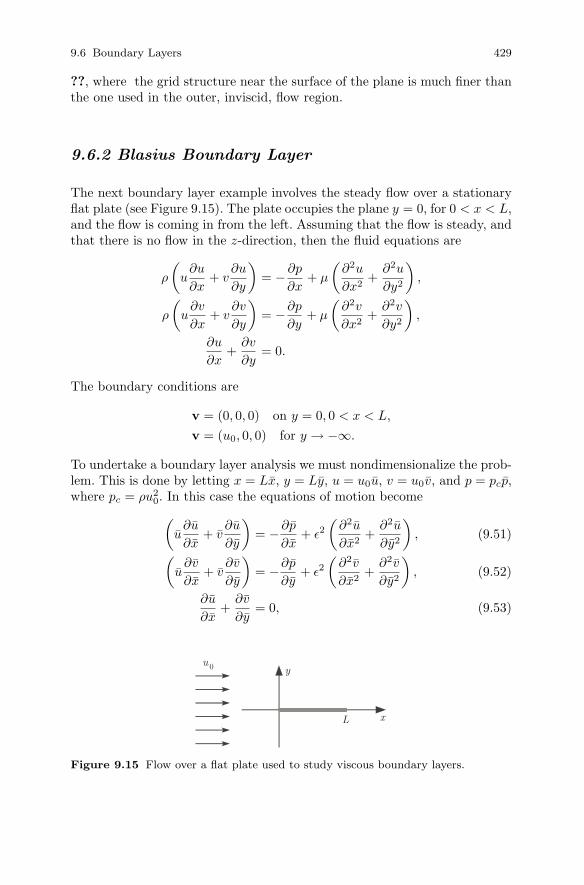
The next boundary layer example involves the steady flow over a stationaryflat plate (see Figure 9.15). The plate occupies the plane y = 0, for 0 < x < L,and the flow is coming in from the left. Assuming that the flow is steady, andthat there is no flow in the z-direction, then the fluid equations are
ρ
(u∂u
∂x+ v
∂u
∂y
)= −∂p
∂x+ µ
(∂2u
∂x2+∂2u
∂y2
),
ρ
(u∂v
∂x+ v
∂v
∂y
)= −∂p
∂y+ µ
(∂2v
∂x2+∂2v
∂y2
),
∂u
∂x+∂v
∂y= 0.
The boundary conditions are
v = (0, 0, 0) on y = 0, 0 < x < L,
v = (u0, 0, 0) for y → −∞.
To undertake a boundary layer analysis we must nondimensionalize the prob-lem. This is done by letting x = Lx, y = Ly, u = u0u, v = u0v, and p = pcp,where pc = ρu2
0. In this case the equations of motion become(u∂u
∂x+ v
∂u
∂y
)= −∂p
∂x+ ε2
(∂2u
∂x2+∂2u
∂y2
), (9.51)(
u∂v
∂x+ v
∂v
∂y
)= −∂p
∂y+ ε2
(∂2v
∂x2+∂2v
∂y2
), (9.52)
∂u
∂x+∂v
∂y= 0, (9.53)
Figure 9.15 Flow over a flat plate used to study viscous boundary layers.

430 9 Fluids
whereε2 =
µ
ρLu0. (9.54)
From (1.20), we have that ε2 = 1/Re. In other words, ε2 is the inverse ofthe Reynolds number for the flow. Our assumption that the viscosity is smalltranslates into the assumption that the Reynolds number is large. As anexample, consider the flow over an airplane wing. The width of the wing onthe Boeing 787 is 18 ft (5.5 m) and cruises at a speed of 561 mph (903 km/h).In this case, Re = 4×10⁷, which certainly qualifies as high Reynolds numberflow.
The reduction of the above problem will closely follow the format used inSection 2.4, although the calculations are a bit more involved.
Outer SolutionThe expansion in this region is assumed to have the form v ∼ v0 + εv1 + · · ·and p ∼ p0 + εp1 + · · · . The problem for the first term, obtained by settingε = 0 in (9.51) - (9.53), is the problem for an inviscid flow. The solution isjust v0 = (u0, 0, 0), and p0 is a constant. It is assumed, for simplicity, thatp0 = 0.
Boundary Layer SolutionThe boundary layer coordinate is
Y =y
ε.
As in Section (2.4), capitals will be used to designate the dependent variablesin the boundary layer region. With this, (9.51) - (9.53) take the form(
U∂U
∂x+
1εV∂U
∂Y
)= −∂P
∂x+ ε2
∂2U
∂x2+∂2U
∂Y 2, (9.55)(
U∂V
∂x+
1εV∂V
∂Y
)= −1
ε
∂P
∂Y+ ε2
∂2V
∂x2+∂2V
∂Y 2, (9.56)
∂U
∂x+
1ε
∂V
∂Y= 0, (9.57)
The appropriate expansions in this case are U ∼ U0 + · · · , V ∼ ε(V0 + · · · ),and P ∼ P0 + · · · . Introducing these into (9.55) - (9.57), and letting ε → 0we obtain (
U0∂U0
∂x+ V0
∂U0
∂Y
)= −∂P0
∂x+∂2U0
∂Y 2, (9.58)
∂P0
∂Y= 0 , (9.59)
∂U0
∂x+∂V0
∂Y= 0. (9.60)

9.6 Boundary Layers 431
From the no-slip condition on the plate, it is required that
(U0, V0) = (0, 0) on Y = 0, 0 < x < 1. (9.61)
Moreover, the solution must match with the outer solution, and for this reasonit is required that
U0 → 1 and P0 → 0 as Y →∞, 0 < x < 1. (9.62)
There is a matching condition for V0, but it is not needed at the moment andthis will be explained after the solution is derived.
From (9.59) and (9.62) it follows that P0 = 0. The usual method for findingthe velocity functions is to introduce a stream function ψ(x, Y ), which isdefined so that
U0 =∂ψ
∂Y, (9.63)
V0 = −∂ψ∂x
. (9.64)
By doing this, the continuity equation (9.57) is satisfied automatically. Thisleaves the momentum equation (9.55), which reduces to
∂ψ
∂Y
∂2ψ
∂Y ∂x− ∂ψ
∂x
∂2ψ
∂Y 2=∂3ψ
∂Y 3. (9.65)
The boundary (9.61) and matching (9.62) conditions transform into the fol-lowing
∂ψ
∂Y=∂ψ
∂x= 0, on Y = 0, (9.66)
and∂ψ
∂Y→ 1, as Y →∞. (9.67)
Something that was not explained above is where the idea of using a streamfunction comes from. The answer is the Helmholtz Representation Theorem(9.22). When the flow is incompressible, and two-dimensional as in the presentexample, then the velocity vector can be written as v = ∇ × g, where g =(0, 0, ψ). Expanding the curl, one obtains v = (∂yψ,−∂xψ, 0), and this givesrise to the stream function.
It is not possible to find an analytical solution of the above problem for thestream function. However, it is possible to come close if we make one moreassumption. Instead of a plate of finite length, we assume that the plate issemi-infinite and occupies the interval 0 ≤ x < ∞. This gives rise to whatis known as the Blasius boundary layer problem, and it can be reduced byintroducing a similarity variable. Specifically, assuming that ψ =
√xf(η),
where η = Y/√x, then (9.65) reduces to

432 9 Fluids
f ′′′ +12ff ′′ = 0, for 0 < η <∞, (9.68)
where (9.66) and (9.67) become
f(0) = f ′(0) = 0, and f ′(∞) = 1. (9.69)
One might argue that we have not made much progress, because the solutionof the above problem is not known. However, the ordinary differential equa-tion (9.68) is certainly simpler than the partial differential equation (9.65),and this does provide some benefit. For example, it is much easier to solve(9.68) numerically than it is to solve (9.65) numerically. Just one last com-ment to make here, before working out an example, is that once the functionf is determined then the velocity functions are calculated using the formulas
U0 = f ′(η), (9.70)
V0 = − 12√x
(f − ηf ′). (9.71)
These expressions are obtained by substituting the similarity solution into(9.63) and (9.64).
Example: Numerical Solution
To use a numerical method to solve (9.68) it is a bit easier to rewrite theequation as a system by letting g = f ′. In this case the equation can bewritten as
00y
−axis
00
x−axis
y−axis
Figure 9.16 Flow over a flat plate, as determined from solving (9.68), (9.69). Theupper graph shows U0, as a function of Y , at three points on the plate. The dashedcurve in the lower graph is where U0 = 0.99.

9.6 Boundary Layers 433
f ′ = g,
g′′ = −12fg′.
The boundary conditions (9.69) become g(0) = 0, g(∞) = 1, and f(0) = 0.With this, it is relatively straightforward to use finite differences to solve theproblem (Holmes [2005]). The result of such a calculation is given in Figure9.16. The upper graph shows the horizontal velocity u at three locations alongthe plate. As required, the velocity is zero on the plate, and as the verticaldistance from the plate increases it approaches the constant velocity of theouter region. It is also evident that the velocity reaches this constant valuefairly quickly for a point on the plate that is near the leading edge, wherex = 0, and less so as the distance from the leading edge increases. The reasonis that the boundary layer on the plate grows with distance from the leadingedge. Using the engineering definition that the boundary layer thickness iswhere the flow reaches 99% of the outer flow value, the dashed curve shownin the lower graph is obtained. The shape of this curve can be explained using(9.71). By definition, the dashed curve is where U0 = 0.99, and this meansthat f ′(η) = 0.99. Letting the solution of this equation be η0 then, becauseη = Y/
√x, we have that the dashed curve is Y = η0
√x.
The above example illustrates how a flow can be separated into an outer,inviscid, region, and a boundary layer where the viscous affects play an im-portant role. This requires a large value for the Reynolds number, and doesnot hold for a low Reynolds number. It is also based on the solution for aninfinitely long plate, something that is rather rare in the real world. Whenthe plate has finite length, a wake is formed downstream from the plate.An example of this is shown in Figure 9.17. The pattern seen in the wake isknown as a Karman vortex street. It is also possible to see the boundary layeron the plate in the upper figure. What is interesting is that the fluid used inthis experiment is water, and not air. This is indicative of the fact that theseparation of the flow into inviscid and boundary layer domains is a charac-
Figure 9.17 Wake behind a flat plate, showing the vortices generated in the flow(Tanaka [1986]). The photograph of the left is the flow immediately behind the plate,and the one on the right is further downstream. The vortices are evident becausealuminum particles are suspended in the flow. In this experiment, Re = 15800.

434 9 Fluids
teristic of any fluid governed by the Navier-Stokes equations, assuming theReynolds number is sufficiently large. It is also evident, given the complexityof the flow, that finding the solution for the finite plate requires numericalmethods. Some of the issues that arise with this are discussed in Cebeci andCousteix [2005].
Before closing this section, a couple of comments are needed about theboundary layer reduction. First, the flow in the immediate vicinity of theleading edge requires a more refined boundary layer analysis that was usedhere. The same comment applies to the trailing edge for the finite length plate.Second, there are questions remaining about the matching requirement forthe vertical velocity. In particular, there must be a matching condition, yetit is not included in (9.62). This is an issue, because according to (9.71), itappears that the vertical velocity is unbounded when one moves out of theboundary layer into the outer region. Namely, given that f ′(∞) = 1 then ηf ′
is unbounded as η → ∞. In comparison, we know that the vertical velocityin the inviscid region is just zero. Therefore, to guarantee that the verticalvelocity matches it must be that f ∼ η as η → ∞. If the solution of (9.68)does not do this then the whole approximation fails. It is found, from thenumerical solution, that f does indeed have the correct limiting behavior,and so the expansions match.
Exercises
9.1. Suppose an incompressible viscous fluid has velocity v = (u, v, 0), withu = ax2 + bxy + cy2, where a, b, and c are constant.
(a) Find v assuming that v(x, 0, z) = 0.(b) Find T.(c) For what values of a, b, and c, if any, is the flow irrotational?
9.2. Suppose the velocity for an incompressible fluid is v = (−αy, αx, β),where α and β are constants.
(a) Show v satisfies the continuity equation.(b) Assuming no external body forces, find the pressure.(c) Is this flow rotational or irrotational?(d) Find the pathlines.(e) This is known as steady helical flow. Why?
9.3. Suppose the velocity for an incompressible fluid is v = (x+ y, 3x− y, 0).(a) Show v satisfies the continuity equation.(b) Assuming no external body forces, find the pressure.(c) Is this flow rotational or irrotational?(d) Find the pathlines.(e) Use the result from part (d) to find the material description of the flow.(f) Find the invariants for D.

Exercises 435
Figure 9.18 Concentric rotating cylinders used in the Taylor-Couette problem inExercise 9.6.
9.4. This problem considers some of the limitations on the method used tosolve the steady flow equations.
(a) Suppose in the Poiseuille flow problem in Section 9.2.2 that the pipe hasan elliptical cross-section. What assumptions about the solution used toderive (9.13) no longer apply? What assumptions should still be valid?
(b) Suppose in the plane Couette flow problem in Section 9.2.1 that gravityis included. This means that a forcing function must be included in (9.2),as determined from (8.77), of the form f = (0,−g, 0). What assumptionsabout the solution used to derive (9.7) no longer apply? What assumptionsshould still be valid?
9.5. As a modification of the plane Couette flow problem, suppose there aretwo fluids between the plates. One fluid occupies the region 0 < y < h0,and has density ρ1 and viscosity ν1. The second fluid occupies the regionh0 < y < h and has density ρ2 and viscosity ν2.
(a) In plane Couette flow the velocity has the form v = (u(y), 0, 0). Also, atthe interface, where y = h0, the velocity and stress are assumed to becontinuous. Use this to show that p, u and u′(y) are continuous at y = h0.
(b) Using the results from part (a), solve this plane Couette problem.
9.6. An incompressible viscous fluid occupies the region between two concen-tric cylinders of radii R1 and R2, where R1 < R2. Assume the cylinders areinfinitely long, and centered on the z-axis (see Figure 9.18). The inner cylin-der is assumed rotating around the z-axis with angular velocity ω1, while theouter cylinder rotates around the z-axis with angular velocity ω2. The flowis assumed to be steady, and there are no body forces. This is known as theTaylor-Couette problem.
(a) Using cylindrical coordinates, explain why the boundary conditions on thecylinders are (vr, vθ, vz) = (0, ωiRi, 0) for r = Ri.
(b) Explain why it is reasonable to assume that the solution has vz = 0 andvr = 0.

436 9 Fluids
(c) Find vθ and p.(d) What is the vorticity for this flow? With this show that the flow is irrota-
tional if R21ω1 = R2
2ω2.
9.7. This problem examines a model for power-law fluids. It is based on theobservation coming from Figure 9.3 that the shear stress for plane Couetteflow has the form T12 = α(∂u
∂y )β . It is assumed here that the fluid is incom-pressible.
(a) In plane Couette flow the velocity has the form v = (u(y), 0, 0). What areD and its three invariants in this case?
(b) As shown in Section 8.10.2.1, the general form of the constitutive law fora nonlinear viscous fluid is T = −pI + G, where G = α0I + α1D + α2D2.Explain how the power-law
T12 = α
∣∣∣∣∂u∂y∣∣∣∣m ∂u
∂y
is obtained by assuming that α0 = α2 = 0 and α1 depends on IID in aparticular way. It is assumed that m > −1, which guarantees that G = 0if D = 0.
(c) Assuming that ∂u∂y > 0, and using the constitutive law from part (b),
solve the resulting plane Couette flow problem. From this show that T12 =αγm+1, where γ is given in (9.8).
(d) On the same axes, sketch T12 as function of γ when −1 < m < 0, whenm = 0, and when 1 < m. Use this to compare the differences in thebehavior of the shear stress for large values of γ. Would the −1 < m < 0case be called a shear-thickening or a shear-thinning situation?
9.8. This problem examines the vorticity for a linear flow, which means thatv = Hx + h, where the matrix H and vector h can dependent on t. Otherproperties of linear flows were developed in Exercises 8.4 and 8.5.
(a) Show that ω = (H32 −H23,H13 −H31,H21 −H12). What is the vorticitywhen H is symmetric?
(b) Show that for rigid body motion, as given in (8.13), H = Q′QT andh = b′−Q′QT b. Therefore, rigid body motion is a special case of a linearflow.
(c) What is v in the case when Q is given in (8.14) and b = 0? For this flowshow that ω = (0, 0, 2ω).
(d) The equations for vortex motion are given in Section 9.3.1. Show that theonly vortex with a smooth velocity and constant vorticity has vθ = 1
2rω.In this case, show that h = 0 and
H =
0 −ω 0
ω 0 0
0 0 0
.

Exercises 437
(e) For the H given in part (d) find a rotation Q so that H = Q′QT . Dothis by showing that this equation reduces to solving Q′′ = H2Q, withQ(0) = I and Q′(0) = H, and then solving for Q. Make sure to verify thatthe solution is a rotation matrix.
(f) Explain why it is possible to conclude that a vortex motion with a smoothvelocity and constant vorticity must be a rigid body motion.
9.9. Suppose that v = α||x||kx, where k and α are real numbers.(a) Show that the flow is irrotational.(b) Find a potential function φ for this flow.(c) Show that this velocity function does not correspond to incompressible
fluid motion, unless α = 0.
9.10. For a Taylor vortex, vr = vz = 0, and
vθ =αr
t2exp(−r2/(4νt)
).
Show this satisfies the equations of motion, assuming the fluid is incompress-ible and there are no body forces. In doing this also determine the pressure.
9.11. For Burger’s vortex, vr = −αr, vz = 2αz, and
vθ =β
r
(1− e−αr2/(2ν)
).
Show this satisfies the equations of motion, assuming the fluid is incompress-ible and there are no body forces. In doing this also determine the pressure.
9.12. This exercise explores the connections between vorticity and energydissipation in a viscous fluid.
(a) The viscous dissipation function Φ is given in (8.110). Show that
Φ = 2µ(D2xx +D2
yy +D2zz + 2D2
xy + 2D2xz + 2D2
yz),
where the Dij ’s are the components of the rate of deformation tensor givenin (8.67).
(b) Show that for an incompressible fluid,
Φ = µω · ω + 2µ∇ · q,
where q = (∇v)v.(c) Let B is a bounded region in space. Use the result from part (b) to derive
what is known as the Bobyleff-Forsyth formula, given as∫∫∫B
ΦdV = µ
∫∫∫B
ω · ω dV + 2µ∫∫∂B
n · q dS.

438 9 Fluids
(d) If v = 0 on ∂B show that∫∫∫B
ΦdV = µ
∫∫∫B
ω · ω dV .
This shows that the total energy dissipation in the region is determinedby the magnitude of the vorticity vector.
(e) Show that for an incompressible fluid, with no body force,
d
dt
∫∫∫R(t)
12ρv · v dV =
∫∫∂R(t)
g · n dS − µ
∫∫∫R(t)
ω · ω dV ,
where g = −pv − µω × v + 2µq, and q is given in part (b).(f) If the fluid is compressible, show that the generalization of the Bobyleff-
Forsyth formula is∫∫∫B
ΦdV =∫∫∫
B
[(λ+ 2µ)Θ2 + µω · ω
]dV + 2µ
∫∫∂B
n · q dS,
where Θ = ∇ · v and q = (∇v)v −Θv.
9.13. There are three known principal invariants, or conserved quantities,for an ideal fluid. One is the circulation, which comes directly from Kelvin’sCirculation Theorem. This problem derives the other two. Assume R(t) is amaterial volume, as used for the Reynolds Transport Theorem, and there areno body forces.
(a) If v · n = 0 on ∂R, show that
d
dt
∫∫∫R
v · v dV = 0.
This is the energy invariant, and states that the kinetic energy of thematerial volume is constant.
(b) If ω · n = 0 on ∂R, show that
d
dt
∫∫∫R
ω · v dV = 0.
This is called the helicity invariant, and it measures the extent the path-lines coil around each other.
(c) Explain why the conclusions of parts (a) and (b) hold if the body forcehas the form f = ∇Ψ .
9.14. Suppose that the velocity of an incompressible fluid is v = v0+ 12Ω×x,
where v0 and Ω are constant vectors. Consequently, v consists of a constant
Exercises 439
velocity v0 added to the velocity for circular motion in the plane perpendic-ular to Ω.
(a) Show that ω = Ω.(b) The helicity density is defined as h = ω ·v, and it gives rise to the invariant
derived in Exercise 9.13(b). Using the result from part (a), show thath = Ω · v0.
(c) Assuming Ω = (0, 0, Ω) and v0 = (0, 0, w0), find the pathlines and fromthis show that the flow is helictical.
(d) From the description of v given above, one might think that it correspondsto rigid body motion. Prove this using the results from Exercises 8.22(d)and 9.8(b).
9.15. In this problem assume the body force in the Navier-Stokes equationscan be written as f = ∇Ψ .
(a) Assuming that the fluid is ideal show that
∂v∂t
+∇(
12v · v +
1ρp− Ψ
)+ ω × v = 0.
In the case where the fluid is also irrotational show that
p = p0(t)− ρ
(∂φ
∂t+
12∇φ · ∇φ
)+ ρΨ.
This is a generalization of Bernoulli’s theorem given in (9.29).(b) Suppose the fluid is inviscid and irrotational. Also, assume it satisfies the
equation of state for a polytropic fluid, which is p = kργ , where γ > 1.Adapt the argument of part (a) to show that
∂φ
∂t+
γ
γ − 1p
ρ+
12∇φ · ∇φ− Ψ = c(t).
9.16. For the impulsive plate problem in Section 9.6.1, suppose the lowerplate moves with velocity v = (u0f(t), 0, 0). Assuming that f(t) is a smoothfunction of t, use the Laplace transform to show that
u(y, t) = u0f(0)erfc(
y
2√νt
)+ u0
∫ t
0
f ′(t− r)erfc(
y
2√νr
)dr.
9.17. For the impulsive plate problem in Section 9.6.1, suppose the lowerplate moves with velocity v = (u0 cos(ωt), 0, 0). This is known as Stokes’second problem. The exact solution can be found using the formula from theprevious problem, but a different approach is taken here.
(a) After a sufficiently long period of time the solution should be approxi-mately periodic. Assume that u = eiωtq(y), where it is understood thatthe real part of this expression is used. This expression should satisfy themomentum equation, and the two boundary conditions. Show that thisresults in the solution of the form u = u0e
−σy cos(σy − ωt).

440 9 Fluids
(b) Sketch the solution as a function of y, and describe the basic characteristicsof the solution.
(c) Show that the boundary layer thickness is approximately 5√
2ν/ω. Whathappens to the thickness as the frequency increases?