chapter 9 randomized algorithms

Chapter 9

Randomized Algorithms

The theme of this chapter israndomized

madendrizo algorithms. These are algorithms that make use ofrandomness in their computation. You might know of quicksort, which is efficient on averagewhen it uses a random pivot, but can be bad for any pivot that is selected without randomness.

Analyzing randomized algorithms can be difficult, so you might wonder why randomiza-tion in algorithms is so important and worth the extra effort. Well it turns out that for certainproblems randomized algorithms are simpler or faster than algorithms that do not use random-ness. The problem of primality testing (PT), which is to determine if an integer is prime, isa good example. In the late 70s Miller and Rabin developed a famous and simple random-ized algorithm for the problem that only requires polynomial work. For over 20 years it wasnot known whether the problem could be solved in polynomial work without randomization.Eventually a polynomial time algorithm was developed, but it is much more complicated andcomputationally more costly than the randomized version. Hence in practice everyone still usesthe randomized version.

There are many other problems in which a randomized solution is simpler or cheaper thanthe best non-randomized solution. In this chapter, after covering the prerequisite background,we will consider some such problems. The first we will consider is the following simple prob-lem:

Question: How many comparisons do we need to find the top two largest numbersin a sequence of n distinct numbers?

Without the help of randomization, there is a trivial algorithm for finding the top two largestnumbers in a sequence that requires about 2n − 3 comparisons. We show, however, that if theorder of the input is randomized, then the same algorithm uses only n+ O(log n) comparisonsin expectation (on average). This matches a more complicated deterministic version based ontournaments.

Randomization plays a particular important role in developing parallel algorithms, and an-alyzing such algorithms introduces some new challenges. In this chapter we will look at two

151

152 CHAPTER 9. RANDOMIZED ALGORITHMS

randomized algorithms with significant parallelism: one for finding the kth smallest element ina sequences, and the other is quicksort. In future chapters we will cover many other randomizedalgorithms.

In this book we will require that randomized algorithms always return the correct answer,but their costs (work and span) will depend on random choices. Such algorithms are sometimescalled Las Vegas algorithms. Algorithms that run in a fixed amount of time, but may or may notreturn the corret answer, depending on random choices, are called Monte Carlo algorithms.

9.1 Discrete Probability: Let’s Toss Some Dice

Not surprisingly analyzing randomized algorithms requires understanding some (discrete) prob-ability. In this section we will cover a variety of ideas that will be useful in analyzing algorithms.

Expected vs. High Probability Bounds. In analyzing costs for a randomized algorithmsthere are two types of bounds that we will find useful: expected bounds, and high-probabilitybounds. Expected bounds basically tell us about the average case across all random choicesused in the algorithm. For example if an algorithm has O(n) expected work, it means that onaverage across all random choices it makes, the algorithm has O(n) work. Once it a while,however, the work could be much larger, for example once in every

√n tries the algorithm

might require O(n3/2) work.

Exercise 9.1. Explain why if an algorithm has Θ(n) expected (average) work it cannotbe the case that once in every n or so tries the algorithm requires Θ(n3) work?

High-probability bounds on the other hand tell us that it is very unlikely that the cost willbe above some bound. Typically the probability is stated in terms of the problem size n. Forexample, we might determine that an algorithm on n elements has O(n) work with probabilityat least 1 − 1/n5. This means that only once in about n5 tries will the algorithm require morethan O(n) work. High-probability bounds are typically stronger than expectation bounds.

Exercise 9.2. Argue that if an algorithm has O(log n) span with probability at least1 − 1/n5, and if its worst case span is O(n), then it must also have O(log n) span inexpectation.

Expected bounds are often very convenient when analyzing work (or running time in tradi-tional sequential algorithms). This is because of the linearity of expectations, discussed furtherbelow. This allows one to add expectations across the components of an algorithm to get theoverall expected work. For example, if we have 100 students and they each take on average 2

April 29, 2015 (DRAFT, PPAP)

9.1. DISCRETE PROBABILITY: LET’S TOSS SOME DICE 153

Figure 9.1: Every year around the mid-dle of April the Computer Science De-partment at Carnegie Mellon Universityholds an event called the “Random Dis-tance Run”. It is a running event aroundthe track, where the official dice tosserrolls a dice immediately before the raceis started. The dice indicates how manyinitial laps everyone has to run. Whenthe first person is about to complete thelaps, a second dice is thrown indicatinghow many more laps everyone has to run.Clearly, some understanding of probabil-ity can help one decide how to practice forthe race and how fast to run at the start.Thanks to Tom Murphy for the design ofthe 2007 T-shirt.

hours to finish an exam, then the total time spent on average across all students (the work) willbe 100× 2 = 200 hours. This makes analysis reasonably easy since it is compositional. Indeedmany textbooks that cover sequential randomized algorithms only cover expected bounds.

Unfortunately such composition does not work when taking a maximum, which is what weneed to analyze span. Again if we had 100 students starting at the same time and they take 2hours on average, we cannot say that the average maximum time across students (the span) is 2hours. It could be that most of the time each student takes 1 hour, but that once on every 100exams or so, each student gets hung up and takes 101 hours. The average for each student is(99× 1 + 1× 101)/100 = 2 hours, but on most exams with a hundred students one student willget hung up, so the expected maximum will be close to 100 hours, not 2 hours. We thereforecannot compose the expected span from each student by taking a maximum. However, if wehave high-probability bounds we can do a sort of composition. Lets say we know that everystudent will finish in 2 hours with probability 1 − 1/n5, or equivalently that they will takemore than two hours with probability 1/n5. Now lets say n students take the exam, what is theprobability that any takes more than 2 hours? It is at most 1/n4, which is still very unlikely. Wewill come back to why when we talk about the union bound.

Because of these properties of summing vs. taking a maximum, in this book we oftenanalyze work using expectation, but analyze span using high probability.

We now describe more formally the probability we require for analyzing randomized algo-rithms. We begin with an example:



Example 9.3. Suppose we have two fair dice, meaning that each is equally likely to landon any of its six sides. If we toss the dice, what is the chance that their numbers sum to4? You can probably figure out that the answer is

# of outcomes that sum to 4# of total possible outcomes

=3

36=

1

12

since there are three ways the dice could sum to 4 (1 and 3, 2 and 2, and 3 and 1), outof the 6× 6 = 36 total possibilities.

Such throwing of dice is called a probabilistic experiment since it is an “experiment” (we canrepeat it many time) and the outcome is probabilistic (each experiment might lead to a differentoutcome).

Discrete probability is really about counting, or possibly weighted counting. In the diceexample we had 36 possibilities and a subset (3 of them) had the property we wanted. Weassumed the dice were unbiased so all possibilities are equally likely. Indeed in general it isuseful to consider all possible outcomes and then count how many of the outcomes match ourcriteria, or perhaps take an average of some value associated with each outcome (e.g. the sumof the values of the two dice). If the outcomes are not equally likely, then the average has tobe weighted by the probability of each outcome. For these purposes we define the notion of asample space (the set of all possible outcomes), primitive events (each element of the samplespace, i.e., each possible outcome), events (subsets of the sample space), probability functions(the probability for each primitive event), and random variables (functions from the samplespace to the real numbers indicating a value associated with the primitive event). We go overeach in turn.

Sample Spaces and Events. A sample space Ω is an arbitrary and possibly infinite (but count-able) set of possible outcomes of a probabilistic experiment. For the dice example, the samplespace is the 36 possible outcomes of the dice. If we are using random numbers, the samplespace corresponds to all possible values of the random numbers used. In the next section weanalyze finding the top two largest elements in a sequence, by using as our sample space allpermutations of the sequence.

A primitive event (or sample point) of a sample space Ω is any one of its elements, i.e. anyone of the outcomes of the random experiment. An event is any subset of Ω and most oftenrepresenting some property common to multiple primitive events. We typically denote eventsby capital letters from the start of the alphabet, e.g. A, B, C.

Probability Functions. A probability function Pr : Ω → [0, 1] is a function that maps eachprimitive event in the sample space to the probability of that primitive event. It must be the casethat the probabilities add to one, i.e.

∑e∈Ω Pr [e] = 1. The probability of an event A is simply



the sum of the probabilities of its primitive events:

Pr [A] =∑e∈A

Pr [e] .

If all probabilities are equal, all we have to do is figure out the size of the event (correspondingset) and divide it by |Ω|. In general this might not be the case. We will use (Ω,Pr) to indicatethe sample space along with its probability function.

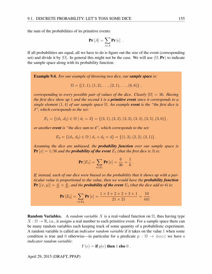
Example 9.4. For our example of throwing two dice, our sample space is:

Ω = (1, 1), (1, 2), . . . , (2, 1), . . . , (6, 6) ,

corresponding to every possible pair of values of the dice. Clearly |Ω| = 36. Havingthe first dice show up 1 and the second 4 is a primitive event since it corresponds to asingle element (1, 4) of our sample space Ω. An example event is the “the first dice is3”, which corresponds to the set:

E1 = (d1, d2) ∈ Ω | d1 = 3 = (3, 1), (3, 2), (3, 3), (3, 4), (3, 5), (3, 6) ,

or another event is “the dice sum to 4”, which corresponds to the set:

E2 = (d1, d2) ∈ Ω | d1 + d2 = 4 = (1, 3), (2, 2), (3, 1) .

Assuming the dice are unbiased, the probability function over our sample space isPr [x] = 1/36 and the probability of the event E1 (that the first dice is 3) is:

Pr [E1] =∑e∈E1

Pr [e] =6

36=

1

6.

If, instead, each of our dice were biased so the probability that it shows up with a par-ticular value is proportional to the value, then we would have the probability functionPr [(x, y)] = x

21× y

21, and the probability of the event E2 (that the dice add to 4) is:

Pr [E2] =∑e∈E2

Pr [e] =1× 3 + 2× 2 + 3× 1

21× 21=

10

441.

Random Variables. A random variable X is a real-valued function on Ω, thus having typeX : Ω→ R, i.e., it assigns a real number to each primitive event. For a sample space there canbe many random variables each keeping track of some quantity of a probabilistic experiment.A random variable is called an indicator random variable if it takes on the value 1 when somecondition is true and 0 otherwise—in particular for a predicate p : Ω → bool we have sindicator random variable:

Y (e) = if p(e) then 1 else 0 .



For a random variable X and a value a ∈ R, we use the following shorthand for the eventcorresponding to X equaling a:

X = a ≡ ω ∈ Ω | X(ω) = a .

We typically denote random variables by capital letters from the end of the alphabet, e.g. X , YZ.

Example 9.5. For throwing two dice, a useful random variables is the sum of the twodice:

X(d1, d2) = d1 + d2 ,

and a useful indicator random variable corresponds to getting doubles (the two dicehave the same value):

Y (d1, d2) = if (d1 = d2) then 1 else 0 .

Using our shorthand, the event X = 4 corresponds to the event “the dice sum to 4”.

We note that the term random variable might seem counter intuitive since it is actually afunction not a variable, and it is not really random at all since it is a well defined deterministicfunction on the sample space. However if you think of it in conjunction with the random ex-periment that selects a primitive element, then it is a variable that takes on its value based on arandom process.

Expectation. We are now ready to talk about expectation. The expectation of a random vari-ableX given a sample space (Ω,Pr) is the sum of the random variable over the primitive eventsweighted by their probability, specifically:

EΩ,Pr

[X] =∑e∈Ω

X(e) · Pr [e] .

One way to think of expectation is as the following higher order function that takes as argumentsthe random variable, along with the sample space and corresponding probability function:

E (Ω,Pr) X = reduce + 0X(e)× Pr [e] : e ∈ Ω

In the notes we will most often drop the (Ω,Pr) subscript on E since it is clear from the context.

We note that it is often not practical to compute expectations directly since the sample spacecan be exponential in the size of the input, or even countably infinite. We therefore resort tovarious shortcuts. For example we can also calculate expectations by considering each value ofa random variable, weighting it by its probability, and summing:

EΩ,Pr

[X] =∑

a∈range of Xa · Pr [X = a] .



Also, the expectation of an indicator random variable Y is the probability that the associatedpredicate p is true (i.e. that Y = 1):

E [Y ] = 0 · Pr [Y = 0] + 1 · Pr [Y = 1]

= Pr [Y = 1] .

Example 9.6. Assuming unbiased dice (Pr [(d1, d2)] = 1/36), the expectation of therandom variable X representing the sum of the two dice is:

EΩ,Pr

[X] =∑

(d1,d2)∈Ω

X(d1, d2)× 1

36=

∑(d1,d2)∈Ω

d1 + d2

36= 7 .

If we bias the coins so that for each dice the probability that it shows up with a particularvalue is proportional to the value, we have Pr′[(d1, d2)] = (d1/21)× (d2/21) and:

EΩ,Pr′

[X] =∑

(d1,d2)∈Ω

((d1 + d2)× d1

21× d2

21

)= 8

2

3,

although that last sum is a bit messy.

Independence. Two events A and B are independent if the occurrence of one does not affectthe probability of the other. This is true if and only if Pr [A ∩B] = Pr [A] · Pr [B]. The proba-bility Pr [A ∩B] is called the joint probability of the events A and B and is sometimes writtenPr [A,B]. When we have multiple events, we say that A1, . . . , Ak are mutually independent ifand only if for any non-empty subset I ⊆ 1, . . . , k,

Pr

[⋂i∈I

Ai

]=∏i∈I

Pr [Ai] .

Example 9.7. For two dice, the events A = (d1, d2) ∈ Ω | d1 = 1 (the first dice is 1)and B = (d1, d2) ∈ Ω | d2 = 1 (the second dice is 1) are independent since

Pr [A]× Pr [B] = 16× 1

6= 1

36

= Pr [A ∩B] = Pr [(1, 1)] = 136.

However, the event C ≡ X = 4 (the dice add to 4) is not independent of A since

Pr [A]× Pr [C] = 16× 3

36= 1

72

6= Pr [A ∩ C] = Pr [(1, 3)] = 136.

A and C are not independent since the fact that the first dice is 1 increases the proba-bility they sum to 4 (from 1

12to 1

6).



Two random variablesX and Y are independent if fixing the value of one does not affect theprobability distribution of the other. This is true if and only if for every a and b the events X =a and Y = b are independent. In our two dice example, a random variable X representingthe value of the first dice and a random variable Y representing the value of the second dice areindependent. However X is not independent of a random variable Z representing the sum ofthe values of the two dice.

Exercise 9.8. For throwing two dice, are the two random variables X and Y in Exam-ple 9.5 independent.

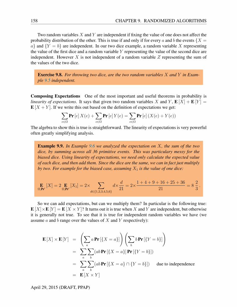
Composing Expectations One of the most important and useful theorems in probability islinearity of expectations. It says that given two random variables X and Y , E [X] + E [Y ] =E [X + Y ]. If we write this out based on the definition of expectations we get:∑

e∈Ω

Pr [e]X(e) +∑e∈Ω

Pr [e]Y (e) =∑e∈Ω

Pr [e] (X(e) + Y (e))

The algebra to show this is true is straightforward. The linearity of expectations is very powerfuloften greatly simplifying analysis.

Example 9.9. In Example 9.6 we analyzed the expectation on X , the sum of the twodice, by summing across all 36 primitive events. This was particulary messy for thebiased dice. Using linearity of expectations, we need only calculate the expected valueof each dice, and then add them. Since the dice are the same, we can in fact just multiplyby two. For example for the biased case, assuming X1 is the value of one dice:

EΩ,Pr′

[X] = 2 EΩ,Pr′

[X1] = 2×∑

d∈1,2,3,4,5,6

d× d

21= 2×1 + 4 + 9 + 16 + 25 + 36

21= 8

2

3.

So we can add expectations, but can we multiply them? In particular is the following true:E [X]×E [Y ] = E [X × Y ]? It turns out it is true whenX and Y are independent, but otherwiseit is generally not true. To see that it is true for independent random variables we have (weassume a and b range over the values of X and Y respectively):

E [X]× E [Y ] =

(∑a

aPr [X = a]

)(∑b

bPr [Y = b]

)=

∑a

∑b

(abPr [X = a] Pr [Y = b])

=∑a

∑b

(abPr [X = a ∩ Y = b]) due to independence

= E [X × Y ]



Example 9.10. Suppose we toss n coins, where each coin has a probability p of comingup heads. What is the expected value of the random variable X denoting the totalnumber of heads?

Solution I: We will apply the definition of expectation directly. This willrely on some messy algebra and useful equalities you might or might notknow, but don’t fret since this not the way we suggest you do it.

E [X] =n∑k=0

k · Pr [X = k]

=n∑k=1

k · pk(1− p)n−k(n

k

)=

n∑k=1

k · nk

(n− 1

k − 1

)pk(1− p)n−k [ because

(n

k

)=n

k

(n− 1

k − 1

)]

= nn∑k=1

(n− 1

k − 1

)pk(1− p)n−k

= nn−1∑j=0

(n− 1

j

)pj+1(1− p)n−(j+1) [ because k = j + 1 ]

= npn−1∑j=0

(n− 1

j

)pj(1− p)(n−1)−j)

= np(p+ (1− p))n [ Binomial Theorem ]= np

That was pretty tedious :(

Solution II: We’ll use linearity of expectations. Let Xi =Ii-th coin turns up heads. That is, 1 if the i-th coin turns up heads and0 otherwise. Clearly, X =

∑ni=1Xi. So then, by linearity of expectations,

E [X] = E

[n∑i=1

Xi

]=

n∑i=1

E [Xi] .

What is the probability that the i-th coin comes up heads? This is exactly p,so E [X] = 0 · (1− p) + 1 · p = p, which means

E [X] =n∑i=1

E [Xi] =n∑i=1

p = np.



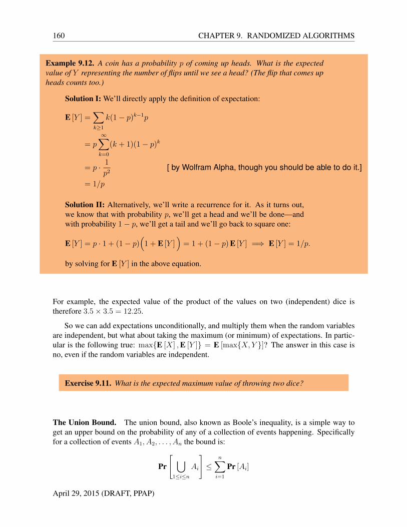
Example 9.12. A coin has a probability p of coming up heads. What is the expectedvalue of Y representing the number of flips until we see a head? (The flip that comes upheads counts too.)

Solution I: We’ll directly apply the definition of expectation:

E [Y ] =∑k≥1

k(1− p)k−1p

= p∞∑k=0

(k + 1)(1− p)k

= p · 1

p2[ by Wolfram Alpha, though you should be able to do it.]

= 1/p

Solution II: Alternatively, we’ll write a recurrence for it. As it turns out,we know that with probability p, we’ll get a head and we’ll be done—andwith probability 1− p, we’ll get a tail and we’ll go back to square one:

E [Y ] = p · 1 + (1− p)(

1 + E [Y ])

= 1 + (1− p) E [Y ] =⇒ E [Y ] = 1/p.

by solving for E [Y ] in the above equation.

For example, the expected value of the product of the values on two (independent) dice istherefore 3.5× 3.5 = 12.25.

So we can add expectations unconditionally, and multiply them when the random variablesare independent, but what about taking the maximum (or minimum) of expectations. In partic-ular is the following true: maxE [X] ,E [Y ] = E [maxX, Y ]? The answer in this case isno, even if the random variables are independent.

Exercise 9.11. What is the expected maximum value of throwing two dice?

The Union Bound. The union bound, also known as Boole’s inequality, is a simple way toget an upper bound on the probability of any of a collection of events happening. Specificallyfor a collection of events A1, A2, . . . , An the bound is:

Pr

[ ⋃1≤i≤n

Ai

]≤

n∑i=1

Pr [Ai]



This bound is true unconditionally, whether the events are independent or not. To see why thebound holds we note that the primitive events in the union on the left are all included in the sumon the right (since the union comes from the same set of events). In fact they might be includedmultiple times in the sum on the right, hence the inequality. In fact sum on the right could addto more than one, in which case the bound is not useful. However, the union bound is veryuseful in generating high-probability bounds, when the probability of each of n events is verylow, e.g. 1/n5 and the sum remains very low, e.g. 1/n4.

Markov’s Inequality. Consider a non-negative random variable X . We can ask how muchlarger can X’s maximum value be than its expected value. With small probability it can be arbi-trarily much larger. However, since the expectation is taken by averaging X over all outcomes,and it cannot take on negative values, X cannot take on a much larger value with significantprobability. If it did it would contribute too much to the sum.

Question 9.13. Can more than half the class do better than twice the average score onthe midterm?

More generally X cannot be a multiple of β larger than its expectation with probability greaterthan 1/β. This is because this part on its own would contribute more than β E [X]× 1

β= E [X]

to the expectation, which is a contradiction. This gives us for a non-negative random variableX the inequality:

Pr[X ≥ β E [X]

]≤ 1

β

or equivalently (by substituting β = α/E [X]),

Pr [X ≥ α] ≤ E [X]

α

which is known as Markov’s inequality.

High-Probability Bounds. As discussed at the start of this section, it can be useful to arguethat some bound on the cost of an algorithm is true with “high probability”, even if not alwaystrue. Unlike expectations, high-probability bounds allow us to compose the span of componentsof algorithms when run in parallel. For a problem of size n we say that some property is truewith high probability if it is true with probability 1−1/nk for some constant k > 1. This meansthe inverse is true with very small probability 1/nk. It is often easier to work with the inverse.Now if we had n experiments each with inverse probability 1/nk we can use the union boundto argue that the total inverse probability is n · 1/nk = 1/nk−1. This means that for k > 2 theprobability 1− 1/nk−1 is still true with high probability.

We now consider how to derive high-probability bounds. We can start by considering theprobability that when flipping n unbiased coins all of them come up heads. This is simply 1/2n



since the sample space is of size 1/2n, each primitive event has equal probability, and only oneof the primitive events has all heads. Certainly asymptotically 1/2n < 1/nk so the fact thatwe will not flip n heads is true with high probability. Even if there are n people each flippingn coins, the probability that no one will flip all heads is still high (at least 1 − n/2n using theunion bound).

Another way to prove high-probability bounds is to use Markov’s inequality. As we will seein Section 9.3 it is sometimes possible to bound the expectation of a random variable X to bevery small, e.g. E [X] ≤ 1/nk. Now using Markov’s inequality we have that the probabilitythat X ≥ 1 is at most 1/nk.

9.2 Finding The Two Largest

The max-two problem is to find the two largest elements from a sequence of n (unique) numbers.Lets consider the following simple algorithm for the problem.

Algorithm 9.14 (Iterative Max-Two).

1 function max2(S) =2 let3 function replace((m1,m2), v) =4 if v ≤ m2 then (m1,m2)5 else if v ≤ m1 then (m1, v)6 else (v,m1)7 val start = if S1 ≥ S2 then (S1, S2) else (S2, S1)8 in9 iter replace start S 〈 3, . . . , n 〉

10 end

We assume S is indexed from 1 to n. In the following analysis, we will be meticulousabout constants. The naıve algorithm requires up to 1 + 2(n− 2) = 2n− 3 comparisons sincethere is one comparison to compute start each of the n − 2 replaces requires up to twocomparisons. On the surface, this may seem like the best one can do. Surprisingly, there is adivide-and-conquer algorithm that uses only about 3n/2 comparisons (exercise to the reader).More surprisingly still is the fact that it can be done in n+O(log n) comparisons. But how?

Puzzle: How would you solve this problem using only n+O(log n) comparisons?

A closer look at the analysis above reveals that we were pessimistic about the number ofcomparisons; not all elements will get past the “if” statement in Line 4; therefore, only some ofthe elements will need the comparison in Line 5. But we didn’t know how many of them, so weanalyzed it in the worst possible scenario.


9.2. FINDING THE TWO LARGEST 163

Let’s try to understand what’s happening better by looking at the worst-case input. Can youcome up with an instance that yields the worst-case behavior? It is not difficult to convinceyourself that there is a sequence of length n that causes this algorithm to make 2n− 3 compar-isons. In fact, the instance is simple: an increasing sequence of length n, e.g., 〈1, 2, 3, . . . , n〉.As we go from left to right, we find a new maximum every time we counter a new element—thisnew element gets compared in both Lines 4 and 5.

But perhaps it’s unlikely to get such a nice—but undesirable—structure if we consider theelements in random order. With only 1 in n! chance, this sequence will be fully sorted. Youcan work out the probability that the random order will result in a sequence that looks “approx-imately” sorted, and it would not be too high. Our hopes are high that we can save a lot ofcomparisons in Line 5 by considering elements in random order.

The algorithm we’ll analyze is the following. On input a sequence T of n elements:

1. Let S = permute(T, π), where π is a random permutation (i.e., we choose one of then! permutations).

2. Run algorithm max2 on S.

Remarks: We don’t need to explicitly construct S. We’ll simply pick a random elementwhich hasn’t been considered and consider that element next until we are done looking at thewhole sequence. For the analysis, it is convenient to describe the process in terms of S.

In reality, the performance difference between the 2n− 3 algorithm and the n− 1 + 2 log nalgorithm is unlikely to be significant—unless the comparison function is super expensive. Formost cases, the 2n− 3 algorithm might in fact be faster to due better cache locality.

The point of this example is to demonstrate the power of randomness in achieving somethingthat otherwise seems impossible—more importantly, the analysis hints at why on a typical “real-world” instance, the 2n−3 algorithm does much better than what we analyzed in the worst case(real-world instances are usually not adversarial).

Analysis

After applying the random permutation we have that our sample space Ω corresponds to eachpermutation. Since there are n! permutations on a sequence of length n and each has equalprobability, we have |Ω| = n! and Pr [e] = 1/n!, e ∈ Ω. However, as we will see, we do notreally need to know this, all we need to know is what fraction of the sample space obeys someproperty.

Let i be the position in S (indexed from 1 to n). Now let Xi be an indicator random variabledenoting whether Line 5 and hence its comparison gets executed for the value at Si (i.e., Recallthat an indicator random variable is actually a function that maps each primitive event (eachpermutation in our case) to 0 or 1. In particular given a permutation, it returns 1 iff for that



permutation the comparison on Line 5 gets executed on iteration i. Lets say we want to nowcompute the total number of comparisons. We can define another random variable (function)Y that for any permutation returns the total number of comparison the algorithm takes on thatpermutation. This can be defined as:

Y (e) = 1︸︷︷︸Line 7

+ n− 2︸︷︷︸Line 4

+n∑i=3

Xi(e)︸︷︷︸Line 5

It is common, however, to use the shorthand notation

Y = 1 + (n− 2) +n∑i=3

Xi

where the argument e and function definition is implied.

We are interested in computing the expected value of Y , that is E [Y ] =∑

e∈Ω Pr [e]Y (e).By linearity of expectation, we have

E [Y ] = E

[1 + (n− 2) +

n∑i=3

Xi

]

= 1 + (n− 2) +n∑i=3

E [Xi] .

Our tasks therefore boils down to computing E [Xi] for i = 3, . . . , n. To compute this expec-tation, we ask ourselves: What is the probability that Si > m2? A moment’s thought showsthat the condition Si > m2 holds exactly when Si is either the largest element or the secondlargest element in S1, . . . , Si. So ultimately we’re asking: what is the probability that Si isthe largest or the second largest element in randomly-permuted sequence of length i?

To compute this probability, we note that each element in the sequence is equally likely tobe anywhere in the permuted sequence (we chose a random permutation. In particular, if welook at the k-th largest element, it has 1/i chance of being at Si. (You should also try to workit out using a counting argument.) Therefore, the probability that Si is the largest or the secondlargest element in S1, . . . , Si is 1

i+ 1

i= 2

i, so

E [Xi] = 1 · 2i

= 2/i.


9.3. FINDING THE KTH SMALLEST ELEMENT 165

Plugging this into the expression for E [Y ], we get

E [Y ] = 1 + (n− 2) +n∑i=3

E [Xi]

= 1 + (n− 2) +n∑i=3

2

i

= 1 + (n− 2) + 2(

13

+ 14

+ . . . 1n

)= n− 4 + 2

(1 + 1

2+ 1

3+ 1

4+ . . . 1

n

)= n− 4 + 2Hn,

where Hn is the n-th Harmonic number. But we know that Hn ≤ 1 + log2 n, so we get E [Y ] ≤n− 2 + 2 log2 n. We could also use the following sledgehammer:

As an aside, the Harmonic sum has the following nice property:

Hn = 1 +1

2+ · · ·+ 1

n= lnn+ γ + εn,

where γ is the Euler-Mascheroni constant, which is approximately 0.57721 · · · , and εn ∼ 12n

,which tends to 0 as n approaches ∞. This shows that the summation and integral of 1/i arealmost identical (up to a small adative constant and a low-order vanishing term).

9.3 Finding The kth Smallest Element

Consider the following problem:

Problem 9.15 (The kth Smallest Element (KS)). Given an α sequence, S, an in-teger k, 0 ≤ k < |S|, and a comparison < defining a total ordering over α, return(sort<(S))k, where sort is the standard sorting problem.

This problem can obviously be implemented using a sort, but this would require O(n log n)work (we assume the comparison takes constant work). Our goal is to do better. In particularwe would like to achieve linear work, while still achieving O(log2 n) span. Here’s where thepower of randomization gives the following simple algorithm.



Algorithm 9.16 (contracting kth smallest).

1 function kthSmallest(k, S) = let2 val p = S0

3 val L = 〈x ∈ S | x < p 〉4 val R = 〈x ∈ S | x > p 〉5 in6 if (k < |L|) then kthSmallest(k, L)7 else if (k < |S| − |R|) then p8 else kthSmallest(k − (|S| − |R|), R)

This algorithm is similar to quicksort but instead of recursing on both sides, it only recurses onone side. Basically it figures out in which side the kth smallest must be in, and just explores thatside. When exploring the right side, R, the k needs to be adjusted by since all elements less orequal to the pivot p are being thrown out: there are |S| − |R| such elements. The algorithm isbased on contraction.

As written the algorithm picks the first key instead of a random key. As with the two-maxproblem, we can add randomness by first randomly permuting a sequence T to generate S andthen applying kthSmallest on S. You should convince yourself that this is equivalent torandomly picking a pivot at each step of contraction.

We now analyze the work and span of this algorithm. Let X = max|L|, |R|/|S|, whichis the fractional size of the larger side. Notice that X is an upper bound on the fractional size ofthe side the algorithm actually recurses into. Now since lines 3 and 4 are simply two filtercalls, we have the following recurrences:

W (n) ≤ W (X · n) + O(n)

S(n) ≤ S(X · n) + O(log n)

Let’s first look at the work recurrence. Specifically, we are interested in E [W (n)]. First,let’s try to get a sense of what happens in expectation.

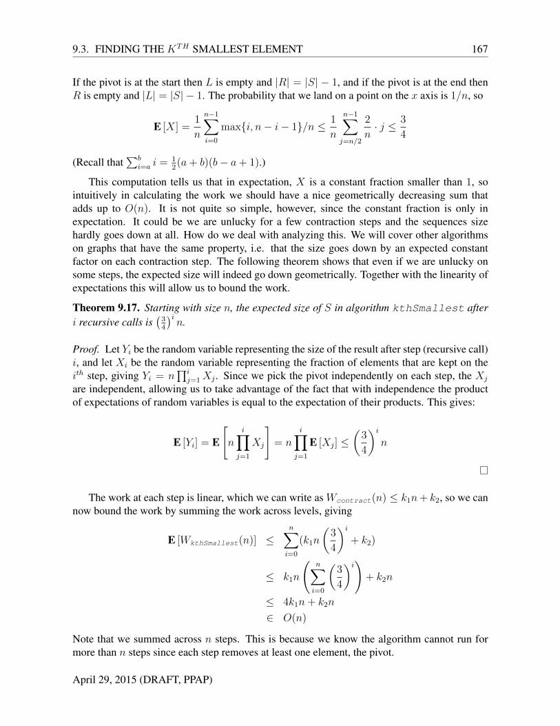
What is the value of E [X]? To understand this we note that all pivots are equally likely. Wecan then draw the following plot of the size of L and size of R as a function of where the pivotbelongs in the sorted order of S.

RL

max(L, R)


9.3. FINDING THE KTH SMALLEST ELEMENT 167

If the pivot is at the start then L is empty and |R| = |S| − 1, and if the pivot is at the end thenR is empty and |L| = |S| − 1. The probability that we land on a point on the x axis is 1/n, so

E [X] =1

n

n−1∑i=0

maxi, n− i− 1/n ≤ 1

n

n−1∑j=n/2

2

n· j ≤ 3

4

(Recall that∑b

i=a i = 12(a+ b)(b− a+ 1).)

This computation tells us that in expectation, X is a constant fraction smaller than 1, sointuitively in calculating the work we should have a nice geometrically decreasing sum thatadds up to O(n). It is not quite so simple, however, since the constant fraction is only inexpectation. It could be we are unlucky for a few contraction steps and the sequences sizehardly goes down at all. How do we deal with analyzing this. We will cover other algorithmson graphs that have the same property, i.e. that the size goes down by an expected constantfactor on each contraction step. The following theorem shows that even if we are unlucky onsome steps, the expected size will indeed go down geometrically. Together with the linearity ofexpectations this will allow us to bound the work.

Theorem 9.17. Starting with size n, the expected size of S in algorithm kthSmallest afteri recursive calls is

(34

)in.

Proof. Let Yi be the random variable representing the size of the result after step (recursive call)i, and let Xi be the random variable representing the fraction of elements that are kept on theith step, giving Yi = n

∏ij=1Xj . Since we pick the pivot independently on each step, the Xj

are independent, allowing us to take advantage of the fact that with independence the productof expectations of random variables is equal to the expectation of their products. This gives:

E [Yi] = E

[n

i∏j=1

Xj

]= n

i∏j=1

E [Xj] ≤(

3

4

)in

The work at each step is linear, which we can write as Wcontract(n) ≤ k1n+ k2, so we cannow bound the work by summing the work across levels, giving

E [WkthSmallest(n)] ≤n∑i=0

(k1n

(3

4

)i+ k2)

≤ k1n

(n∑i=0

(3

4

)i)+ k2n

≤ 4k1n+ k2n

∈ O(n)

Note that we summed across n steps. This is because we know the algorithm cannot run formore than n steps since each step removes at least one element, the pivot.



We now use Theorem 9.17 to bound the number of steps taken by kthSmallest to muchbetter than n using high probability bounds. This will allow us to bound the span of the algo-rithm. Consider step i = 10 log2 n. In this case we have the expected size upper bounded byn(

34

)10 log2 n, which with a little math is the same as n×n−10 log2(4/3) ≈ n−3.15. We can now useMarkov’s inequality and observe that if the expected size is at most n−3.15 then the probabilityof having size at least 1 (if less than 1 then the algorithm is done) is bounded by:

Pr[Y10 log2 n ≥ 1

]≤ E[Y10 log2 n]/1 = n−3.15

This is a high probability bound as discussed at the start of Section 9.1. By increasing 10 to20 we can decrease the probability to n−7.15, which is extremely unlikely: for n = 106 this is10−42. We have therefore show that the number of steps is O(log n) with high probability. Eachstep has span O(log n) so the overall span is O(log2 n) with high probability.

In summary, we have shown than the kthSmallest algorithm on input of size n doesO(n) work in expectation and has O(log2 n) span with high probability. As mentioned at thestart of Section 9.1 we will typically be analyzing work using expectation and span using highprobability.

Exercise 9.18. Show that the high probability bounds on span for kthSmallest im-ply equivalent bounds in expectation.

9.4 Quicksort

You have surely seen quicksort before. The purpose of this section is to analyze the work andspan of quicksort. In later chapters we will see that the analysis of quicksort presented here isis effectively identical to the analysis of a certain type of balanced tree called Treaps. It is alsothe same as the analysis of “unbalanced” binary search trees under random insertion.

Quicksort is one of the earliest and most famous algorithms. It was invented and analyzed byTony Hoare around 1960. This was before the big-O notation was used to analyze algorithms.Hoare invented the algorithm while an exchange student at Moscow State University whilestudying probability under Kolmogorov—one of the most famous researchers in probabilitytheory. The analysis we will cover is different from what Hoare used in his original paper,although we will mention how he did the analysis. It is interesting that while Quicksort isoften used as an quintessential example of a recursive algorithm, at the time, no programminglanguage supported recursion and Hoare spent significant space in his paper explaining how tosimulate recursion with a stack.

Consider the quicksort algorithm given in Algorithm 9.19. In this algorithm, we intention-ally leave the pivot-choosing step unspecified because the property we are discussing holdsregardless of the choice of the pivot.


9.4. QUICKSORT 169

Algorithm 9.19 (Quicksort).

1 function sort(S) =2 if |S| = 0 then S3 else let4 val p = pick a pivot from S5 val S1 = 〈 s ∈ S | s < p 〉6 val S2 = 〈 s ∈ S | s = p 〉7 val S3 = 〈 s ∈ S | s > p 〉8 val (R1, R3) = (sort(S1) || sort(S3))9 in

10 append(R1, append(S2, R3))11 end

Question 9.20. Is there parallelism in quicksort?

There is plenty of parallelism in this version quicksort.1 There is both parallelism due to thetwo recursive calls and in the fact that the filters for selecting elements greater, equal, and lessthan the pivot can be parallel.

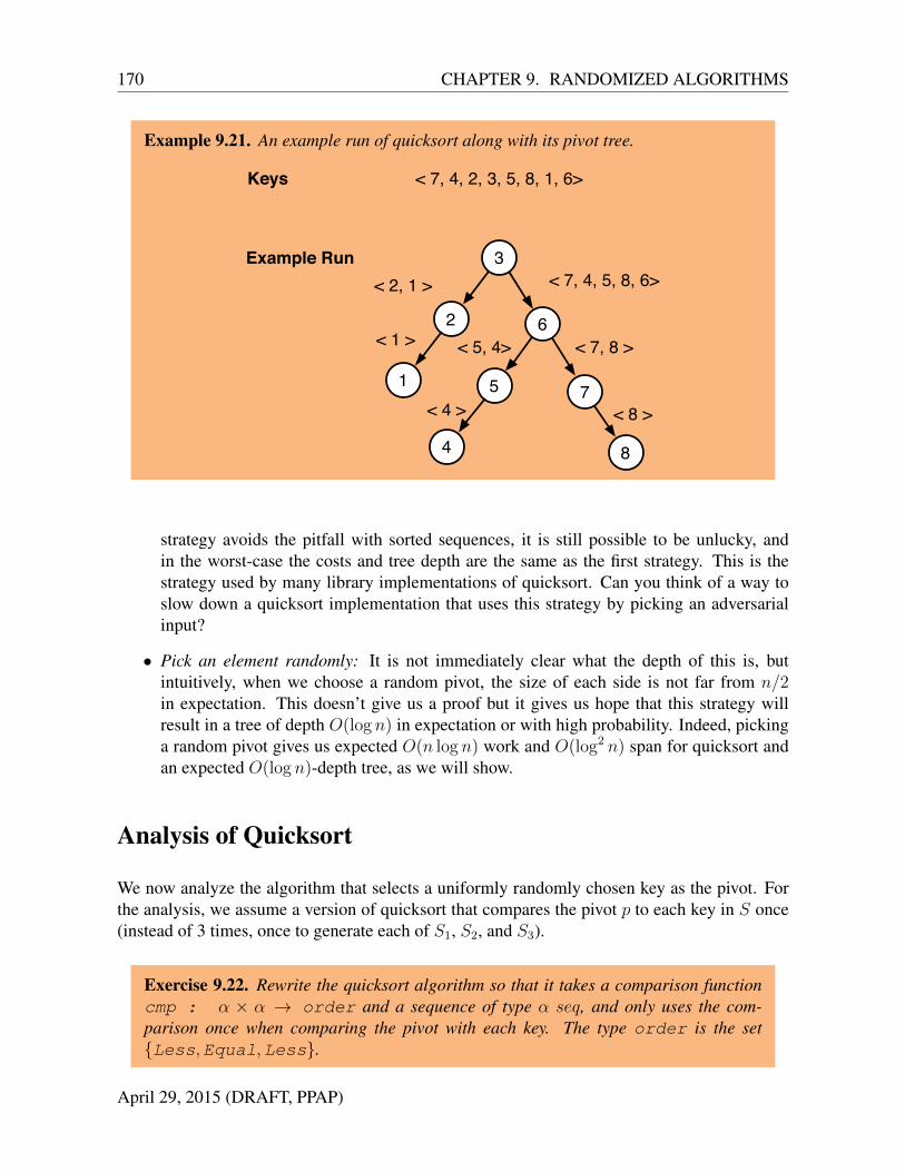
Note that each call to quicksort either makes no recursive calls (the base case) or two recur-sive calls. The call tree is therefore binary. We will often find it convenient to map the run ofa quicksort to a binary-search tree (BST) representing the recursive calls along with the pivotschosen. We will sometimes refer to this tree as the call tree or pivot tree. We will use this call-tree representation to reason about the properties of quicksort, e.g., the comparisons performed,its span. An example is shown in Example 9.21.

Let’s consider some strategies for picking a pivot.

• Always pick the first element: If the sequence is sorted in increasing order, then pickingthe first element is the same as picking the smallest element. We end up with a lopsidedrecursion tree of depth n. The total work is O(n2) since n− i keys will remain at level iand hence we will do n− i− 1 comparisons at that level for a total of

∑n−1i=0 (n− i− 1).

Similarly, if the sequence is sorted in decreasing order, we will end up with a recursiontree that is lopsided in the other direction. In practice, it is not uncommon for a sortfunction input to be a sequence that is already sorted or nearly sorted.

• Pick the median of three elements: Another strategy is to take the first, middle, and thelast elements and pick the median of them. For sorted lists the split is even, so each sidecontains half of the original size and the depth of the tree is O(log n). Although this

1This differs from Hoare’s original version which sequentially partitioned the input by the pivot using twofingers that moved from each end and swapping two keys whenever a key was found on the left greater than thepivot and on the right less than the pivot.



Example 9.21. An example run of quicksort along with its pivot tree.

3

2

1

6

5

4

7

8

Keys

Example Run

< 7, 4, 2, 3, 5, 8, 1, 6>

< 7, 4, 5, 8, 6>< 2, 1 >

< 1 > < 7, 8 >< 5, 4>

< 4 > < 8 >

strategy avoids the pitfall with sorted sequences, it is still possible to be unlucky, andin the worst-case the costs and tree depth are the same as the first strategy. This is thestrategy used by many library implementations of quicksort. Can you think of a way toslow down a quicksort implementation that uses this strategy by picking an adversarialinput?

• Pick an element randomly: It is not immediately clear what the depth of this is, butintuitively, when we choose a random pivot, the size of each side is not far from n/2in expectation. This doesn’t give us a proof but it gives us hope that this strategy willresult in a tree of depth O(log n) in expectation or with high probability. Indeed, pickinga random pivot gives us expected O(n log n) work and O(log2 n) span for quicksort andan expected O(log n)-depth tree, as we will show.

Analysis of Quicksort

We now analyze the algorithm that selects a uniformly randomly chosen key as the pivot. Forthe analysis, we assume a version of quicksort that compares the pivot p to each key in S once(instead of 3 times, once to generate each of S1, S2, and S3).

Exercise 9.22. Rewrite the quicksort algorithm so that it takes a comparison functioncmp : α × α → order and a sequence of type α seq, and only uses the com-parison once when comparing the pivot with each key. The type order is the setLess,Equal,Less.


9.4. QUICKSORT 171

In the analysis, for picking the pivots, we are going to use a priority-based selection technique.Before the start of the algorithm, we’ll pick for each key a random priority uniformly at randomfrom the real interval [0, 1] such that each key has a unique priority. We then pick in Line ??the key with the highest priority. Notice that once the priorities are decided, the algorithm iscompletely deterministic.

Example 9.23. Quicksort with priorities and its call tree, which is a binary-search-tree,illustrated.

3

2

1

6

5

4

7

8

Keys

Example Run

< 7, 4, 2, 3, 5, 8, 1, 6 >

< 7, 4, 5, 8, 6>< 2, 1 >

< 1 > < 7, 8 >< 5, 4>

< 4 > < 8 >

Priorities < 0.3, 0.2, 0.7, 0.8, 0.4, 0.1, 0.5 , 0.6 >

Exercise 9.24. Convince yourself that the two presentations of randomized quicksortare fully equivalent (modulo the technical details about how we might store the priorityvalues).

Before we get to the analysis, let’s observe some properties of quicksort. For these obser-vations, it might be helpful to consider the example shown above. In quicksort, a comparisonalways involves a pivot and another key. Since, the pivot is never sent to a recursive call, a keyis selected as a pivot exactly once, and is not involved in further comparisons (after is becomesa pivot). Before a key is selected as a pivot, it may be compared to other pivots, once per pivot,and thus two keys are never compared more than once.

Question 9.25. Can you tell which keys are compared by looking at just the call tree?

Following the discussion above, we note that a key is compared with all its ancestors in the calltree, and all its descendants in the call tree.

Question 9.26. Let x and z two keys such that x < z. Suppose that a key y is selectedas a pivot before either x or z is selected. Are x and z compared?

When the algorithm selects a key (y) in between two keys (x, z) as a pivot, it sends the twokeys to two separate subtrees. The two keys (x and z) separated in this way are never comparedagain.



Question 9.27. Suppose that the keys x and y are adjacent in the sorted order, howmany times are they compared?

Adjacent keys are compared exactly once. This is the case because there is no key that will everseparate them.

Question 9.28. Would it be possible to modify quicksort so that it never compares ad-jacent keys?

Indeed adjacent keys must be compared by any sorting algorithm since otherwise it would beimpossible to tell which one appears first in the output.

Question 9.29. Based on these observations, can you bound the number of comparisonsperformed by quicksort in terms of the comparisons between keys.

The total number of comparisons can be written by summing over all comparisons involvingeach key. Since each key is involved in a comparison with another key at most once, the totalnumber of comparisons can be expressed as the sum over all pairs of keys. That is, we can justconsider each pair of key once and check whether they are ancestors/descendants or not and addone to our sum if so.

Expected work for randomized quicksort. We are now ready to analyze the expected workof randomized quicksort by counting how many comparisons quicksort it makes in expec-tation. We introduce a random variable

Xn = # of comparisons quicksort makes on input of size n,

and we are interested in finding an upper bound on E [Xn]. In particular we will show it is inO(n log n). E [Xn] will not depend on the order of the input sequence.

For our analysis we will consider the final sorted order of the keys T = sort(S). In thisterminology, we’ll also denote by pi the priority we chose for the element Ti. We’ll derive anexpression forXn by breaking it up into a bunch of random variables and bound them. Considertwo positions i, j ∈ 1, . . . , n in the sequence T (the output ordering). We define followingrandom variable:

Aij =

1 if Ti and Tj are compared by quicksort0 otherwise

Based on the discussion in the previous section, we can write Xn by summing over all Aij’s:

Xn ≤n∑i=1

n∑j=i+1

Aij


9.4. QUICKSORT 173

Ti T j

pp pp

=

p

=

Figure 9.2: The possible relationships between the selected pivot p, Ti and Tj illustrated.

Note that we only need to consider the case that i < j since we only want to count eachcomparison once. By linearity of expectation, we have

E [Xn] ≤n∑i=1

n∑j=i+1

E [Aij]

Furthermore, since each Aij is an indicator random variable, E [Aij] = Pr [Aij = 1]. Ourtask therefore comes down to computing the probability that Ti and Tj are compared (i.e.,Pr [Aij = 1]) and working out the sum.

To compute this probability, let’s take a closer look at the quicksort algorithm to gathersome intuitions. Notice that the top level takes as its pivot p the element with highest priority.Then, it splits the sequence into two parts, one with keys larger than p and the other with keyssmaller than p. For each of these parts, we run quicksort recursively; therefore, inside it,the algorithm will pick the highest priority element as the pivot, which is then used to split thesequence further.

For any one call to quicksort there are three possibilities (illustrated in Figure 9.2) forAij , where i < j:

• The pivot (highest priority element) is either Ti or Tj , in which case Ti and Tj are com-pared and Aij = 1.

• The pivot is element between Ti and Tj , in which case Ti is in S1 and Tj is in S3 and Tiand Tj will never be compared and Aij = 0.

• The pivot is less than Ti or greater than Tj . Then Ti and Tj are either both in S1 or bothin S3, respectively. Whether Ti and Tj are compared will be determined in some laterrecursive call to quicksort.

Let us first consider the first two cases when the pivot is one of Ti, Ti+1, ..., Tj . With thisview, the following observation is not hard to see:

Claim 9.30. For i < j, Ti and Tj are compared if and only if pi or pj has the highestpriority among pi, pi+1, . . . , pj.



Proof. Assume first that Ti (Tj) has the highest priority. In this case, all the elements in thesubsequence Ti . . . Tj will move together in the call tree until Ti (Tj) is selected as pivot. Whenit is, Ti and Tj will be compared. This proves the first half of the theorem.

For the second half, assume that Ti and Tj are compared. For the purposes of contradiction,assume that there is a key Tk, i < k < j with a higher priority between them. In any collectionof keys that include Ti and Tj , Tk will become a pivot before either of them. Since Ti ≤Tk ≤ Tj it will separate Ti and Tj into different buckets, so they are never compared. This is acontradiction; thus we conclude there is no such Tk.

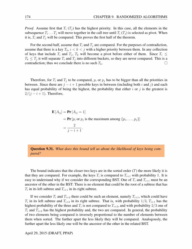
Therefore, for Ti and Tj to be compared, pi or pj has to be bigger than all the priorities inbetween. Since there are j − i + 1 possible keys in between (including both i and j) and eachhas equal probability of being the highest, the probability that either i or j is the greatest is2/(j − i+ 1). Therefore,

E [Aij] = Pr [Aij = 1]

= Pr [pi or pj is the maximum among pi, . . . , pj]

=2

j − i+ 1.

Question 9.31. What does this bound tell us about the likelihood of keys being com-pared?

The bound indicates that the closer two keys are in the sorted order (T ) the more likely it isthat they are compared. For example, the keys Ti is compared to Ti+1 with probability 1. It iseasy to understand why if we consider the corresponding BST. One of Ti and Ti+1 must be anancestor of the other in the BST: There is no element that could be the root of a subtree that hasTi in its left subtree and Ti+1 in its right subtree.

If we consider Ti and Ti+2 there could be such an element, namely Ti+1, which could haveTi in its left subtree and Ti+2 in its right subtree. That is, with probability 1/3, Ti+1 has thehighest probability of the three and Ti is not compared to Ti+2, and with probability 2/3 one ofTi and Ti+2 has the highest probability and, the two are compared. In general, the probabilityof two elements being compared is inversely proportional to the number of elements betweenthem when sorted. The further apart the less likely they will be compared. Analogously, thefurther apart the less likely one will be the ancestor of the other in the related BST.


9.4. QUICKSORT 175

Hence, the expected number of comparisons made in randomized quicksort is

E [Xn] ≤n−1∑i=1

n∑j=i+1

E [Aij]

=n−1∑i=1

n∑j=i+1

2

j − i+ 1

=n−1∑i=1

n

n−i+1∑k=2

2

k

≤ 2n−1∑i=1

Hn

= 2nHn ∈ O(n log n)

(Recall: Hn = lnn+O(1).)

Indirectly, we have also shown that the average work for the basic deterministic quicksort(always pick the first element) is also O(n log n). Just shuffle the data randomly and then applythe basic quicksort algorithm. Since shuffling the input randomly results in the same input aspicking random priorities and then reordering the data so that the priorities are in decreasing or-der, the basic quicksort on that shuffled input does the same operations as randomized quicksorton the input in the original order. Thus, if we averaged over all permutations of the input thework for the basic quicksort is O(n log n) on average.

An alternative analysis of work. Another way to analyze the work of quicksort is to writea recurrence for the expected work (number of comparisons) directly. This is the approachtaken by Tony Hoare in his original paper. For simplicity we assume there are no equal keys(equal keys just reduce the cost). The recurrence for the number of comparisons X(n) done byquicksort is then:

X(n) = X(Yn) +X(n− Yn − 1) + n− 1

where the random variable Yn is the size of the set S1 (we use X(n) instead of Xn to avoiddouble subscrips). We can now write an equation for the expectation of X(n).

E [X(n)] = E [X(Yn) +X(n− Yn − 1) + n− 1]

= E [X(Yn)] + E [X(n− Yn − 1)] + n− 1

=1

n

n−1∑i=0

(E [X(i)] + E [X(n− i− 1)]) + n− 1

where the last equality arises since all positions of the pivot are equally likely, so we can justtake the average over them. This can be by guessing the answer and using substitution. It givesthe same result as our previous method. We leave this as exercise.



Span of Quicksort. We now analyze the span of quicksort. All we really need to calculate isthe depth of the pivot tree, since each level of the tree has span O(log n)—needed for the filter.We argue that the depth of the pivot tree is O(log n) by relating it to the number of contractionsteps of the randomized kthSmallest we considered in Section 9.3. The refer to the ith nodeof the pivot tree as the node corresponding to the ith smallest key. This is also the ith node in anin-order traversal.

Claim 9.32. The path from the root to the ith node of the pivot tree is the same as thesteps of kthSmallest on k = i. That is to the say that the distribution of pivotsselected and the sizes of each problem is identical. [NEEDS A BIT MORE EXPLANA-TION.]

The reason this is true, is that kthSmallest is the same as quicksort except we only godown one of the two recursive branches—the branch that contains the kth key. We are almostdone now since we showed that the number of steps of kthSmallest will be more than10 lg n with probability at most 1/n3.15. We might be tempted to say immediately that thereforethe probability that quicksort has any node of depth 10 lg n is also 1/n3.15. This is wrong.

Question 9.33. Why is it wrong?

It is wrong because all we have analyzed is that each node had depth greater than 10 lg n withprobability at most 1/n3.15. Since we have multiple nodes the probably increases that at leastone will go above the bound. Here is where we get to apply the union bound. Recall theunion bound says the probability of the union of a bunch of events is at most the sum of theprobabilities of the events. In our case the individual events are the depths of each node beinglarger 10 lg n, and the union is the probability that any of the nodes has depth larger than 10 lg n.There are n events each with probability 1/n3.15, so the union bound states that:

Pr [depth of quicksort pivot tree > 10 lg n] ≤ n

n3.15=

1

n2.15

We thus have our high probability bounds on the depth.

The overall span of randomized quicksort is therefore O(log2 n) with high probability.


chapter 9 randomized algorithms

Documents