chapter 9 the existence, strength, and direction of an

BIVARIATE ANALYSIS

Chapter 9 The Existence, Strength, andDirection of an Association

In Chapters 7 and 8, we looked at the relationships between pairs of variables.There are three big questions you should ask about a statistical relationship. First,is there evidence of its existence? If so, then there is a second question: What is itsstrength? Third, in a relationship involving variables measured at the ordinal,interval, or ratio level, what is its direction? In this chapter, we’ll look at ways ofunderstanding the existence, strength, and direction of relationships betweenvariables.

In our previous discussions, you may have been frustrated over the ambigu-ity as to what constitutes a strong or a weak relationship. Ultimately, there is noabsolute answer to this question. The strength or significance of a relationshipbetween two variables depends on many things, but we’ll try to pin down thebasic answers.

If you are trying to account for differences between people on some variable,such as their attitudes about the death penalty, the explanatory power of one vari-able, such as education, must be contrasted with the explanatory power of othervariables. So you might be interested in knowing whether education, politicalaffiliation, or region of upbringing has the greatest impact on a person’s attitudesabout the death penalty.

Sometimes the importance of a relationship is based on practical policy impli-cations. Thus the impact of some variable in explaining (and potentially reducing)auto theft rates, for example, might be converted to a matter of dollars. Does thevery popular anti–drug abuse program Project DARE actually bring about anymeasurable decline in drug or alcohol abuse among young people? Other relation-ships might be expressed in terms of lives saved, students graduating fromcollege, and so forth.

In this chapter, we address another standard for judging the significance ofrelationships between variables, one commonly used by social scientists.Whenever analyses are based on samples selected from a population rather thanon data collected from everyone in that population, there is always the possibilitythat what we learn from the samples may not truly reflect the whole population.Thus we might discover that women are more religious than men in a sample, butthat could simply be an artifact of our sample: We happened to pick too many reli-gious women or too few religious men.

139

09-Logio-45507.qxd 1/28/2008 3:53 PM 39

Social scientists often test the statistical significance of relationships discov-ered between variables. Although this does not constitute a direct measure of thestrength of a relationship, it tells us the likelihood that the observed relationshipcould have resulted from the vagaries of probability sampling, which we call sam-pling error. These tests relate to the strength of relationships in that the strongeran observed relationship, the less likely it is that it could be the result of samplingerror. Likewise, it is more probable that the observed relationship representssomething that exists in the population as a whole.

9.1 Chi-Square

To learn the logic of statistical significance, let’s begin with a measure, chi-square,that is based on the kinds of crosstabulations we’ve been examining in previouschapters. For a concrete example, we’ll return to one of the tables that examinesthe relationship between religion and abortion attitudes.

Let’s reexamine the relationship between religious affiliation and uncondi-tional support for abortion.

Do a crosstab of ABANY (row variable) and RELIGCAT (column variable),with cells percentaged by column.

The question this table is designed to answer is whether a person’s religiousaffiliation affects his or her attitude toward abortion. You’ll recall that we con-cluded it does: Catholics and Protestants are the most opposed to abortion, andpeople with no religion or “other” religion are the most supportive. The questionwe now confront is whether the observed differences point to some genuine pat-tern in the U.S. population at large or if they result from a quirk of sampling.

To assess the observed relationship, we are going to begin by asking whatwe should have expected to find if there were no relationship between religiousaffiliation and abortion attitudes. An important part of the answer lies in the

140 Bivariate Analysis

09-Logio-45507.qxd 1/28/2008 3:53 PM Page 140

rightmost column in the table. It indicates that 48.3% of the whole sample sup-ported a woman’s unconditional right to an abortion and 51.7% did not.

If there were no relationship between religious affiliation and abortion atti-tudes, we should expect to find 48.3% of the Protestants approving, 48.3% of theCatholics approving, 48.3% of the Jews approving, and so forth. But recall that theearlier results did not match this perfect model of no relationship. So the questionis whether the disparity between the model and our observations falls within thenormal degree of sampling error.

To measure the extent of the disparity between the model and what’s beenobserved, we need to calculate the number of cases we’d expect in each cell of thetable if there were no relationship. The following table shows how to calculate theexpected cell frequencies.

ABANY Protestant Catholic Jewish None Other

Approve 144 109 10 62 21× 0.483 × 0.483 × 0.483 × 0.483 × 0.483

Disapprove 144 109 10 62 21× 0.517 × 0.517 × 0.517 × 0.517 × 0.517

If there were no relationship between religious affiliation and abortion atti-tudes, we would expect that 48.3% of the 144 Protestants (144 × 0.483 = 70) wouldapprove and 51.7% of the 144 Protestants (144 × 0.517 = 74) would disapprove. Ifyou continue this series of calculations, you should arrive at the following set ofexpected cell frequencies.


Approve 70 53 5 30 10Disapprove 74 56 5 32 11

The next step in calculating chi-square is to calculate the difference betweenexpected and observed values in each cell of the table. For example, if religion hadno effect on abortion, we would have expected to find 70 Protestants approving;in fact, we observed only 68. Thus the discrepancy in that cell is –2. The discrep-ancy for Catholics approving is –15 (observed – expected = 38 – 53). The follow-ing table shows the discrepancies for each cell.


Approve –2 –15 3 11 2Disapprove 2 15 –3 –11 –2

Finally, for each cell, we square the discrepancy and divide it by the expectedcell frequency. For the Protestants approving of abortion, then, the squared discrep-ancy is 4 (–2 × –2). Dividing it by the expected frequency of 70 yields 0.06 (roundedoff a bit). When we repeat this for each cell, we get the following results:

Chapter 9: The Existence, Strength, and Direction of an Association 141

09-Logio-45507.qxd 1/28/2008 3:53 PM Page 141


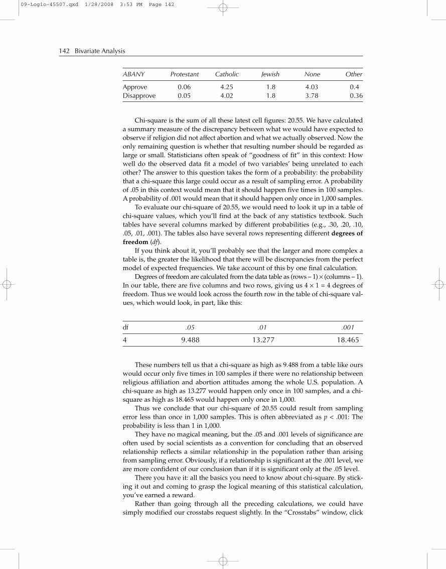
Approve 0.06 4.25 1.8 4.03 0.4Disapprove 0.05 4.02 1.8 3.78 0.36

Chi-square is the sum of all these latest cell figures: 20.55. We have calculateda summary measure of the discrepancy between what we would have expected toobserve if religion did not affect abortion and what we actually observed. Now theonly remaining question is whether that resulting number should be regarded aslarge or small. Statisticians often speak of “goodness of fit” in this context: Howwell do the observed data fit a model of two variables’ being unrelated to eachother? The answer to this question takes the form of a probability: the probabilitythat a chi-square this large could occur as a result of sampling error. A probabilityof .05 in this context would mean that it should happen five times in 100 samples.A probability of .001 would mean that it should happen only once in 1,000 samples.

To evaluate our chi-square of 20.55, we would need to look it up in a table ofchi-square values, which you’ll find at the back of any statistics textbook. Suchtables have several columns marked by different probabilities (e.g., .30, .20, .10,.05, .01, .001). The tables also have several rows representing different degrees offreedom (df).

If you think about it, you’ll probably see that the larger and more complex atable is, the greater the likelihood that there will be discrepancies from the perfectmodel of expected frequencies. We take account of this by one final calculation.

Degrees of freedom are calculated from the data table as (rows – 1) × (columns – 1).In our table, there are five columns and two rows, giving us 4 × 1 = 4 degrees offreedom. Thus we would look across the fourth row in the table of chi-square val-ues, which would look, in part, like this:

df .05 .01 .001

4 9.488 13.277 18.465

These numbers tell us that a chi-square as high as 9.488 from a table like ourswould occur only five times in 100 samples if there were no relationship betweenreligious affiliation and abortion attitudes among the whole U.S. population. Achi-square as high as 13.277 would happen only once in 100 samples, and a chi-square as high as 18.465 would happen only once in 1,000.

Thus we conclude that our chi-square of 20.55 could result from samplingerror less than once in 1,000 samples. This is often abbreviated as p < .001: Theprobability is less than 1 in 1,000.

They have no magical meaning, but the .05 and .001 levels of significance areoften used by social scientists as a convention for concluding that an observedrelationship reflects a similar relationship in the population rather than arisingfrom sampling error. Obviously, if a relationship is significant at the .001 level, weare more confident of our conclusion than if it is significant only at the .05 level.

There you have it: all the basics you need to know about chi-square. By stick-ing it out and coming to grasp the logical meaning of this statistical calculation,you’ve earned a reward.

Rather than going through all the preceding calculations, we could havesimply modified our crosstabs request slightly. In the “Crosstabs” window, click


09-Logio-45507.qxd 1/28/2008 3:53 PM Page 142

“Statistics” and select “Chi-square” in the upper left corner of the window. Thenrun the “Crosstabs” request.

We are interested primarily in the first row of figures in this report. Notice thatthe 20.524 value of chi-square is slightly different from our hand calculation. Thisis due to our rounding off in our cell calculations and shouldn’t worry you. Noticethat we’re told there are 4 degrees of freedom. Finally, SPSS has calculated theprobability of getting a chi-square this high with 4 degrees of freedom and has runout of space after five zeros to the right of the decimal point. Thus the probabilityis far less than .001, as we determined by checking a table of chi-square values.

The reference to a “minimum expected frequency” of 4.83 (found under thechi-square table) is worth noting. Because the calculation of chi-square involvesdivisions by expected cell frequencies, it can be greatly inflated if any of them arevery small. By convention, adjustments to chi-square should be made if more than20% of the expected cell frequencies are below 5. You should check a statistics textif you want to know more about this.

While it is fresh in your mind, why don’t you have SPSS calculate some morechi-squares for you? For example, why don’t you see what the chi-square is for therelationship between SEX and ABANY?

To experiment more with chi-square, you might rerun some of the other tablesrelating various demographic variables to abortion attitudes. Notice that chi-square offers a basis for comparing the relative importance of different variablesin determining attitudes on this controversial topic.

It bears repeating here that tests of significance are different from measures ofassociation, although they are related. The stronger an association between twovariables, the more likely it is that the association will be judged statisticallysignificant—that is, not a simple product of sampling error. Other factors alsoaffect statistical significance, however. As we’ve already mentioned, the number


09-Logio-45507.qxd 1/28/2008 3:53 PM Page 143

of degrees of freedom in a table is relevant. So is the size of the sample: The largerthe sample, the more likely the association is to be judged significant.

Researchers often distinguish between statistical significance (examined inthis section) and substantive significance. The latter refers to the importance of anassociation, and it can’t be determined by empirical analysis alone. As we sug-gested at the outset of this chapter, substantive significance depends on practicaland theoretical factors. All this notwithstanding, social researchers often find sta-tistical significance a useful device in gauging associations.

Whereas chi-square operates on the logic of the contingency table, whichyou’ve grown accustomed to through the crosstabs procedure, we’re going to turnnext to a test of significance based on means.

9.2 t-Tests

Who do you suppose lives longer, men or women? Whichever group lives longershould have a higher average age at any given time. Regardless of whether youknow the answer to this question for the U.S. population as a whole, let’s seewhether our GSS data can shed some light on the issue.

We could find the average ages of men and women in our GSS sample withthe simple command path

Analyze → Compare Means → Means

Because age is the characteristic we want to compare men and women on,AGE is the dependent variable and SEX the independent. Transfer those variablesto the appropriate fields in the window. Then click “OK.”


09-Logio-45507.qxd 1/28/2008 3:53 PM Page 144

As you can see, our sample reflects the general population in that womenhave a mean age of 45.45, compared with 44.02 for men. The task facing us nowparallels the one pursued in the discussion of chi-square. Does the observeddifference reflect a pattern that exists in the whole population, or is it simply aresult of a sampling procedure that happened to get too many old women or toomany young men this time? Would another sample indicate that men are olderthan women or that there is no difference?

Given that we’ve moved very deliberately through the logic and calculationsof chi-square, we are going to avoid such details in the present discussion. Thet-test examines the distribution of values on one variable (age) among differentgroups (men and women) and calculates the probability that the observed differ-ence in means results from sampling error alone.

To request a t-test from SPSS to examine the relationship between AGE andSEX, you enter the following command path:

Analyze → Compare Means → Independent-Samples T-Test


09-Logio-45507.qxd 1/28/2008 3:53 PM Page 145

In this window, we want to enter AGE as the “Test Variable” and SEX as the“Grouping Variable.” This means that SPSS will group respondents by sex andthen examine and compare the mean ages of the two groups.

Notice that when you enter the “Grouping Variable,” SPSS puts “SEX[??]” inthat field. Although the comparison groups are obvious in the case of SEX, theymight not be so obvious with other variables, so SPSS wants some guidance. Click“Define Groups.”

Type 1 into “Group 1” and 2 into “Group 2.” Click “Continue” and then “OK.”


09-Logio-45507.qxd 1/28/2008 3:53 PM Page 146

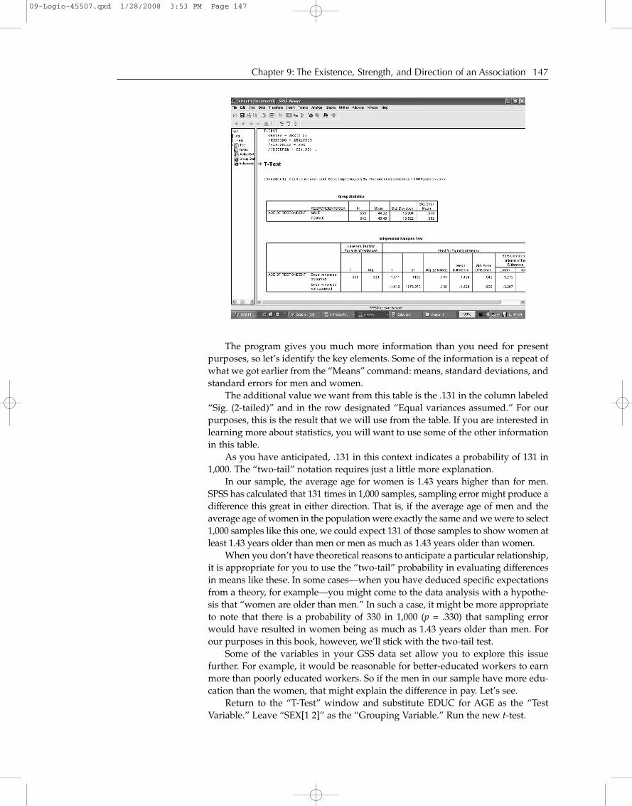
The program gives you much more information than you need for presentpurposes, so let’s identify the key elements. Some of the information is a repeat ofwhat we got earlier from the “Means” command: means, standard deviations, andstandard errors for men and women.

The additional value we want from this table is the .131 in the column labeled“Sig. (2-tailed)” and in the row designated “Equal variances assumed.” For ourpurposes, this is the result that we will use from the table. If you are interested inlearning more about statistics, you will want to use some of the other informationin this table.

As you have anticipated, .131 in this context indicates a probability of 131 in1,000. The “two-tail” notation requires just a little more explanation.

In our sample, the average age for women is 1.43 years higher than for men.SPSS has calculated that 131 times in 1,000 samples, sampling error might produce adifference this great in either direction. That is, if the average age of men and theaverage age of women in the population were exactly the same and we were to select1,000 samples like this one, we could expect 131 of those samples to show women atleast 1.43 years older than men or men as much as 1.43 years older than women.

When you don’t have theoretical reasons to anticipate a particular relationship,it is appropriate for you to use the “two-tail” probability in evaluating differencesin means like these. In some cases—when you have deduced specific expectationsfrom a theory, for example—you might come to the data analysis with a hypothe-sis that “women are older than men.” In such a case, it might be more appropriateto note that there is a probability of 330 in 1,000 (p = .330) that sampling errorwould have resulted in women being as much as 1.43 years older than men. Forour purposes in this book, however, we’ll stick with the two-tail test.

Some of the variables in your GSS data set allow you to explore this issuefurther. For example, it would be reasonable for better-educated workers to earnmore than poorly educated workers. So if the men in our sample have more edu-cation than the women, that might explain the difference in pay. Let’s see.

Return to the “T-Test” window and substitute EDUC for AGE as the “TestVariable.” Leave “SEX[1 2]” as the “Grouping Variable.” Run the new t-test.


09-Logio-45507.qxd 1/28/2008 3:53 PM Page 147

What conclusion do you draw from these latest results? Notice first that themen and women in our sample have a slightly different mean number of years ofeducation. This fact is confirmed by the probability reported: The difference issmall and could be expected by chance alone in about 91 samples in 1,000 (p = .091).

In concluding from this that men do not have significantly more educationthan women, we rule out that education is a legitimate reason for women earningless than men. That’s not to say that there aren’t other legitimate reasons that mayaccount for a gender difference in pay. For instance, it is often argued that womentend to concentrate in less prestigious jobs than men: nurses rather than doctors,secretaries rather than executives, teachers rather than principals. Leaving asidethe reasons for such occupational differences, that might account for the differ-ences in pay. As you may recall, your GSS data contain a measure of socioeco-nomic status (SEI). We used that variable in our experimentation withcorrelations. Let’s see whether the women in our sample have less prestigiousjobs, on the average, than the men.

Go back to the “T-Test” window and replace EDUC with SEI. Run the proce-dure, and you should get the following result.


09-Logio-45507.qxd 1/28/2008 3:53 PM Page 148

The mean difference in socioeconomic index ratings of men and women is 2.3on a scale from 0 to 100. Moreover, SPSS tells us that such a difference could beexpected as a consequence of sampling error in about 55 samples in 1,000 (p =.055). Gender evidently is not the reason women earn less.

To pursue this line of inquiry further, you will need additional analytic skills,which will be covered shortly in our discussion of multivariate analysis.

If you want to experiment more with t-tests, you might substitute RACE forSEX in the commands we’ve been sending to SPSS. If you do that, realize that youhave asked SPSS to consider only code categories 1 and 2 on SEX; applied to RACE,that will limit the comparison to whites and blacks, omitting the “other” category.

9.3 Analysis of Variance

The t-test is limited to the comparison of two groups at a time. If we wanted tocompare the levels of education of different religious groups, we’d have to com-pare Protestants and Catholics, Protestants and Jews, Catholics and Jews, and soforth. And if some of the comparisons found significant differences and othercomparisons did not, we’d be hard-pressed to reach an overall conclusion aboutthe nature of the relationship between the two variables.

The analysis of variance (ANOVA) is a technique that resolves the shortcom-ing of the t-test. It examines the means of subgroups in the sample and analyzesthe variances as well. That is, it examines more than whether the actual values areclustered around the mean or spread out from it.

If we were to ask ANOVA to examine the relationship between RELIGCATand EDUC, it would determine the mean years of education for each of the differ-ent religious groups, noting how they differed from one another. Those between-group differences would be compared with the within-group differences(variance), such as how much Protestants differed among themselves. Both setsof comparisons are reconciled by ANOVA to calculate the likelihood thatthe observed differences are merely the result of sampling error.


09-Logio-45507.qxd 1/28/2008 3:53 PM Page 149

To get a clearer picture of ANOVA, ask SPSS to perform the analysis we’vebeen discussing. You can probably figure out how to do that, but here’s a hint:

Analyze → Compare Means → One-Way ANOVA

Put EDUC into the “Dependent” list and RELIGCAT in the “Factor” field.Launch the procedure.

Here’s the SPSS report on the analysis. Again, we’ve gotten more informa-tion than we want for our present purposes. For our immediate purposes, let’s


09-Logio-45507.qxd 1/28/2008 3:53 PM Page 150

look simply at the row titled “Between Groups.” This refers to the amount ofvariance in EDUC that can be explained by variations in RELIG. We have intro-duced you to ANOVA because we feel it is useful and we wanted to open upfor you the possibility of your using this popular technique; however, you willneed more specialized training in the performance of analysis of variance to useit effectively.

9.4 Summary

This chapter has taken on the difficult question of whether the observed relation-ship between two variables is important. It is natural that you would want toknow whether and when you have discovered something worth writing homeabout. No one wants to shout, “Look what I’ve discovered!” and have others say,“That’s no big thing.”

We’ve presented several statistics that help resolve whether a relationshipexists between two variables. We’ve also seen that the level of measurement of thevariables determines which statistic to use and how much we learn about theassociation. For nominal-level variables, we can learn only whether a relationshipexists. For ordinal variables, we can learn whether it exists and in what direction(positive or negative). For interval- and ratio-level variables, we have a lot moreinformation, and we learn not only about existence and direction but also aboutthe strength of the relationship.

Ultimately, there is no simple test of the substantive significance of a relation-ship between variables. If we found that women earn less than men, who can saywhether that amounts to a lot less or just a little bit less? In a more precise study,we could calculate exactly how much less in dollars, but we would still not be ina position to say absolutely whether that amount was a lot or a little. If womenmade a dollar a year less than men on the average, we’d all probably agree thatthat was not an important difference. Conversely, if we learned that men earneda hundred times as much as women, we’d probably all agree that that was a bigdifference. Few of the differences we discover in social science research are thatdramatic, however.

In this chapter, we’ve examined a very specific approach that social scientistsoften take in addressing the issue of significance. As distinct from notions ofsubstantive significance, we have examined statistical significance. In each of themeasures we’ve examined—chi-square, t-test, and analysis of variance—we’veasked how likely it would be that sampling error could produce the observed rela-tionship if there were actually no relationship in the population from which thesample was drawn.

This assumption of no relationship is sometimes called the null hypothe-sis. The tests of significance we’ve examined all deal with the probability thatthe null hypothesis is correct. If the probability is high, we conclude thatthere is no relationship between the two variables under study in the wholepopulation.

If the probability is small that the null hypothesis could be true, we concludethat the observed relationship reflects a genuine pattern in the population.


09-Logio-45507.qxd 1/28/2008 3:53 PM Page 151

Key Terms


Student Study Site

Log on to the Web-based student study site at http://www.sagepub.com/logiostudy for access tothe data sets referred to in the text and additional study resources.

analysis of variance (ANOVA)chi-squaredegrees of freedom (df)null hypothesis

sampling errorstatistical significancesubstantive significancet-test

09-Logio-45507.qxd 1/28/2008 3:53 PM Page 152

chapter 9 the existence, strength, and direction of an

Documents