chapter 9files.openscad.org/tutorial/chapter_9.pdf · chapter 9 doing math calculations in openscad...

Chapter 9

Doing math calculations in OpenSCAD

So far you have learned that OpenSCAD variables can hold only one value throughout the

execution of a script, the last value that has been assigned to them. You have also learned that a

common use of OpenSCAD variables is to provide parameterization of your models. In this case

every parameterized model would have a few independent variables, whose values you can

change to tune that model. These variables are usually directly assigned a value as in the

following examples.

…

wheel_diameter = 12;

…

body_length = 70;

…

wheelbase = 40;

…

// etc.

…

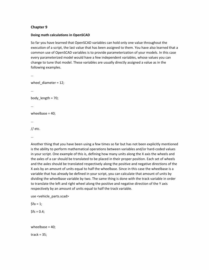
Another thing that you have been using a few times so far but has not been explicitly mentioned

is the ability to perform mathematical operations between variables and/or hard-coded values

in your script. One example of this is, defining how many units along the X axis the wheels and

the axles of a car should be translated to be placed in their proper position. Each set of wheels

and the axles should be translated respectively along the positive and negative directions of the

X axis by an amount of units equal to half the wheelbase. Since in this case the wheelbase is a

variable that has already be defined in your script, you can calculate that amount of units by

dividing the wheelbase variable by two. The same thing is done with the track variable in order

to translate the left and right wheel along the positive and negative direction of the Y axis

respectively by an amount of units equal to half the track variable.

use <vehicle_parts.scad>

$fa = 1;

$fs = 0.4;

wheelbase = 40;

track = 35;

translate([-wheelbase/2, track/2]) simple_wheel();

translate([-wheelbase/2, -track/2]) simple_wheel();

translate([-wheelbase/2, 0, 0])axle(track=track);

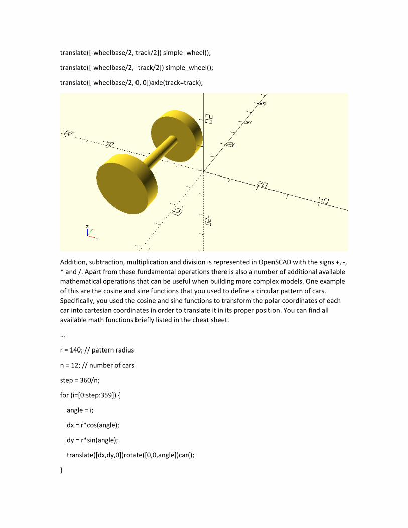
Addition, subtraction, multiplication and division is represented in OpenSCAD with the signs +, -,

* and /. Apart from these fundamental operations there is also a number of additional available

mathematical operations that can be useful when building more complex models. One example

of this are the cosine and sine functions that you used to define a circular pattern of cars.

Specifically, you used the cosine and sine functions to transform the polar coordinates of each

car into cartesian coordinates in order to translate it in its proper position. You can find all

available math functions briefly listed in the cheat sheet.

…

r = 140; // pattern radius

n = 12; // number of cars

step = 360/n;

for (i=[0:step:359]) {

angle = i;

dx = r*cos(angle);

dy = r*sin(angle);

translate([dx,dy,0])rotate([0,0,angle])car();

}

…

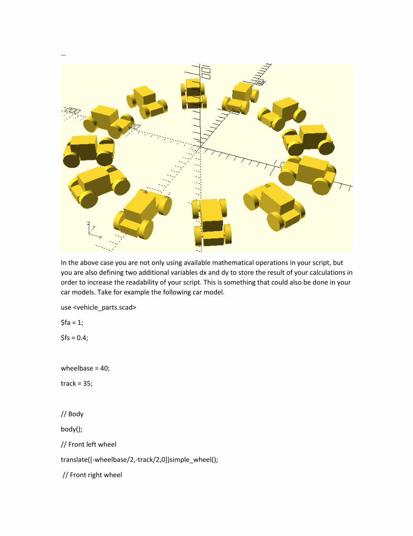
In the above case you are not only using available mathematical operations in your script, but

you are also defining two additional variables dx and dy to store the result of your calculations in

order to increase the readability of your script. This is something that could also be done in your

car models. Take for example the following car model.


$fa = 1;

$fs = 0.4;

wheelbase = 40;

track = 35;

// Body

body();

// Front left wheel

translate([-wheelbase/2,-track/2,0])simple_wheel();

// Front right wheel

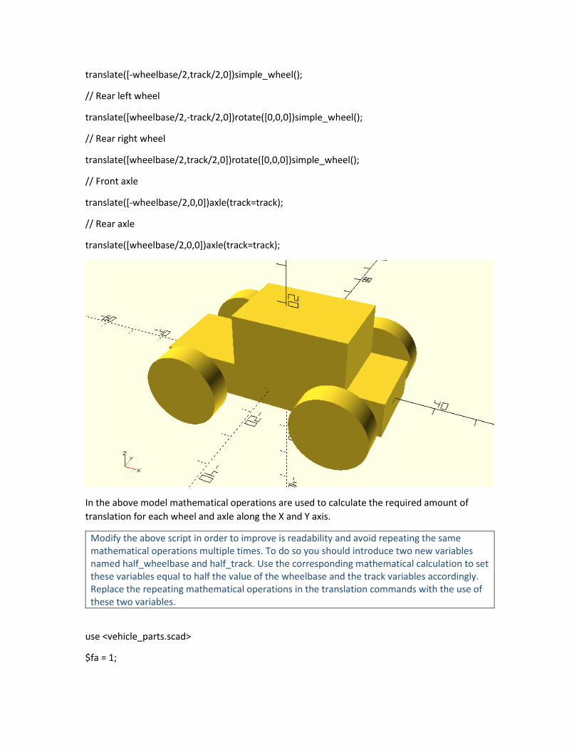
translate([-wheelbase/2,track/2,0])simple_wheel();

// Rear left wheel

translate([wheelbase/2,-track/2,0])rotate([0,0,0])simple_wheel();

// Rear right wheel

translate([wheelbase/2,track/2,0])rotate([0,0,0])simple_wheel();

// Front axle

translate([-wheelbase/2,0,0])axle(track=track);

// Rear axle

translate([wheelbase/2,0,0])axle(track=track);

In the above model mathematical operations are used to calculate the required amount of

translation for each wheel and axle along the X and Y axis.

Modify the above script in order to improve is readability and avoid repeating the same mathematical operations multiple times. To do so you should introduce two new variables named half_wheelbase and half_track. Use the corresponding mathematical calculation to set these variables equal to half the value of the wheelbase and the track variables accordingly. Replace the repeating mathematical operations in the translation commands with the use of these two variables.


$fa = 1;

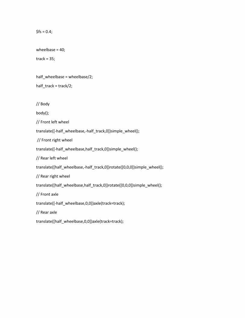
$fs = 0.4;

wheelbase = 40;

track = 35;

half_wheelbase = wheelbase/2;

half_track = track/2;

// Body

body();

// Front left wheel

translate([-half_wheelbase,-half_track,0])simple_wheel();

// Front right wheel

translate([-half_wheelbase,half_track,0])simple_wheel();

// Rear left wheel

translate([half_wheelbase,-half_track,0])rotate([0,0,0])simple_wheel();

// Rear right wheel

translate([half_wheelbase,half_track,0])rotate([0,0,0])simple_wheel();

// Front axle

translate([-half_wheelbase,0,0])axle(track=track);

// Rear axle

translate([half_wheelbase,0,0])axle(track=track);

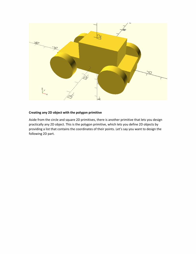
Creating any 2D object with the polygon primitive

Aside from the circle and square 2D primitives, there is another primitive that lets you design

practically any 2D object. This is the polygon primitive, which lets you define 2D objects by

providing a list that contains the coordinates of their points. Let’s say you want to design the

following 2D part.

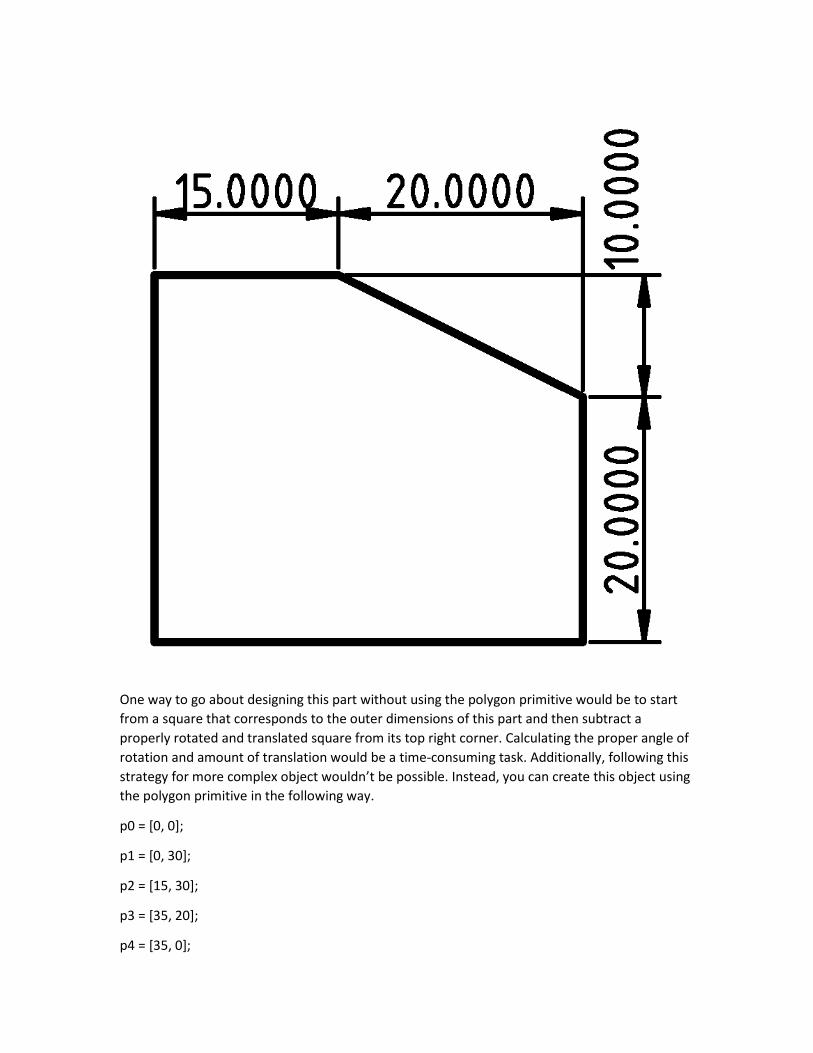
One way to go about designing this part without using the polygon primitive would be to start

from a square that corresponds to the outer dimensions of this part and then subtract a

properly rotated and translated square from its top right corner. Calculating the proper angle of

rotation and amount of translation would be a time-consuming task. Additionally, following this

strategy for more complex object wouldn’t be possible. Instead, you can create this object using

the polygon primitive in the following way.

p0 = [0, 0];

p1 = [0, 30];

p2 = [15, 30];

p3 = [35, 20];

p4 = [35, 0];

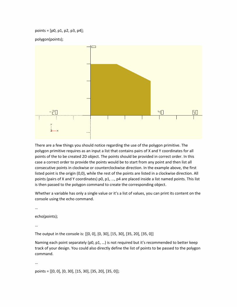
points = [p0, p1, p2, p3, p4];

polygon(points);

There are a few things you should notice regarding the use of the polygon primitive. The

polygon primitive requires as an input a list that contains pairs of X and Y coordinates for all

points of the to be created 2D object. The points should be provided in correct order. In this

case a correct order to provide the points would be to start from any point and then list all

consecutive points in clockwise or counterclockwise direction. In the example above, the first

listed point is the origin (0,0), while the rest of the points are listed in a clockwise direction. All

points (pairs of X and Y coordinates) p0, p1, …, p4 are placed inside a list named points. This list

is then passed to the polygon command to create the corresponding object.

Whether a variable has only a single value or it’s a list of values, you can print its content on the

console using the echo command.

…

echo(points);

…

The output in the console is: [[0, 0], [0, 30], [15, 30], [35, 20], [35, 0]]

Naming each point separately (p0, p1, …) is not required but it’s recommended to better keep

track of your design. You could also directly define the list of points to be passed to the polygon

command.

…

points = [[0, 0], [0, 30], [15, 30], [35, 20], [35, 0]];

…

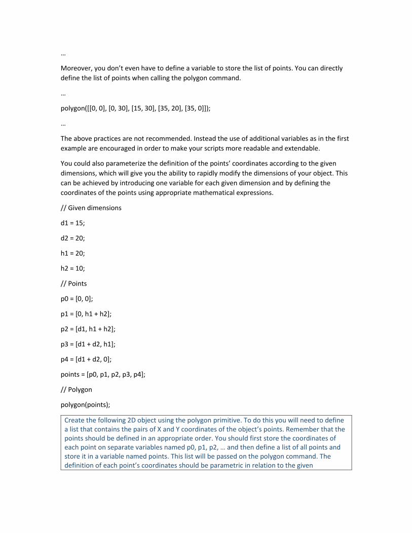
Moreover, you don’t even have to define a variable to store the list of points. You can directly

define the list of points when calling the polygon command.

…

polygon([[0, 0], [0, 30], [15, 30], [35, 20], [35, 0]]);

…

The above practices are not recommended. Instead the use of additional variables as in the first

example are encouraged in order to make your scripts more readable and extendable.

You could also parameterize the definition of the points’ coordinates according to the given

dimensions, which will give you the ability to rapidly modify the dimensions of your object. This

can be achieved by introducing one variable for each given dimension and by defining the

coordinates of the points using appropriate mathematical expressions.

// Given dimensions

d1 = 15;

d2 = 20;

h1 = 20;

h2 = 10;

// Points

p0 = [0, 0];

p1 = [0, h1 + h2];

p2 = [d1, h1 + h2];

p3 = [d1 + d2, h1];

p4 = [d1 + d2, 0];

points = [p0, p1, p2, p3, p4];

// Polygon

polygon(points);

Create the following 2D object using the polygon primitive. To do this you will need to define a list that contains the pairs of X and Y coordinates of the object’s points. Remember that the points should be defined in an appropriate order. You should first store the coordinates of each point on separate variables named p0, p1, p2, … and then define a list of all points and store it in a variable named points. This list will be passed on the polygon command. The definition of each point’s coordinates should be parametric in relation to the given

dimensions which can be achieved by using appropriate mathematical expressions. To do this you will also need to define a variable for each given dimension.

// Given dimensions

h1 = 23;

h2 = 10;

h3 = 8;

d1 = 25;

d2 = 12;

d3 = 15;

// Points

p0 = [0, 0];

p1 = [0, h1 + h2];

p2 = [d3, h1];

p3 = [d1 + d2, h1 + h2];

p4 = [d1 + d2, h3];

p5 = [d1, 0];

points = [p0, p1, p2, p3, p4, p5];

// Polygon

polygon(points);

Using the linear_extrude and rotate_extrude commands create a tube and a ring respectively that have the above profile. The tube should have a height of 100 units. The ring should have an inner diameter of 100 units. How many units do you need to translate the 2d profile along the positive direction of the X axis to achieve this?

…

linear_extrude(height=100)polygon(points);

…

…

rotate_extrude(angle=360)translate([50,0,0])polygon(points);

…

Challenge

It’s time to use your new skills to create the body of a racing car!

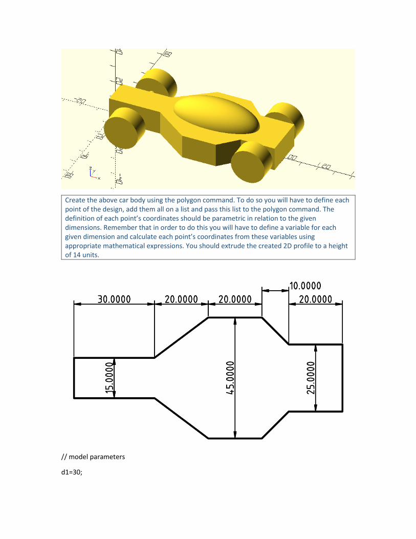
Create the above car body using the polygon command. To do so you will have to define each point of the design, add them all on a list and pass this list to the polygon command. The definition of each point’s coordinates should be parametric in relation to the given dimensions. Remember that in order to do this you will have to define a variable for each given dimension and calculate each point’s coordinates from these variables using appropriate mathematical expressions. You should extrude the created 2D profile to a height of 14 units.

// model parameters

d1=30;

d2=20;

d3=20;

d4=10;

d5=20;

w1=15;

w2=45;

w3=25;

h=14;

// right side points

p0 = [0, w1/2];

p1 = [d1, w1/2];

p2 = [d1 + d2, w2/2];

p3 = [d1 + d2 + d3, w2/2];

p4 = [d1 + d2 + d3 + d4, w3/2];

p5 = [d1 + d2 + d3 + d4 + d5, w3/2];

// left side points

p6 = [d1 + d2 + d3 + d4 + d5, -w3/2];

p7 = [d1 + d2 + d3 + d4, -w3/2];

p8 = [d1 + d2 + d3, -w2/2];

p9 = [d1 + d2, -w2/2];

p10 = [d1, -w1/2];

p11 = [0, -w1/2];

// all points

points = [p0, p1, p2, p3, p4, p5, p6, p7, p8, p9, p10, p11];

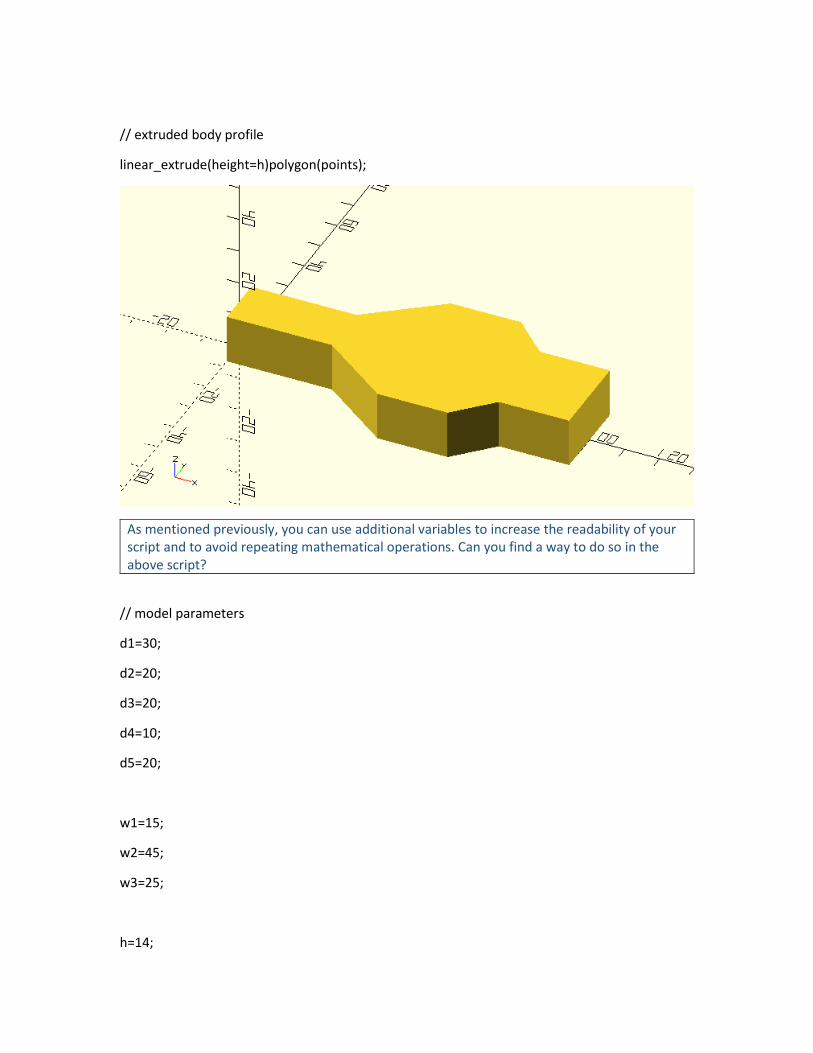
// extruded body profile

linear_extrude(height=h)polygon(points);

As mentioned previously, you can use additional variables to increase the readability of your script and to avoid repeating mathematical operations. Can you find a way to do so in the above script?

// model parameters

d1=30;

d2=20;

d3=20;

d4=10;

d5=20;

w1=15;

w2=45;

w3=25;

h=14;

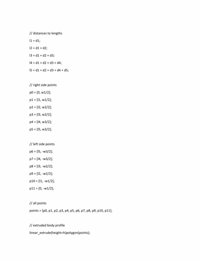
// distances to lengths

l1 = d1;

l2 = d1 + d2;

l3 = d1 + d2 + d3;

l4 = d1 + d2 + d3 + d4;

l5 = d1 + d2 + d3 + d4 + d5;


p0 = [0, w1/2];

p1 = [l1, w1/2];

p2 = [l2, w2/2];

p3 = [l3, w2/2];

p4 = [l4, w3/2];

p5 = [l5, w3/2];

// left side points

p6 = [l5, -w3/2];

p7 = [l4, -w3/2];

p8 = [l3, -w2/2];

p9 = [l2, -w2/2];

p10 = [l1, -w1/2];

p11 = [0, -w1/2];

// all points




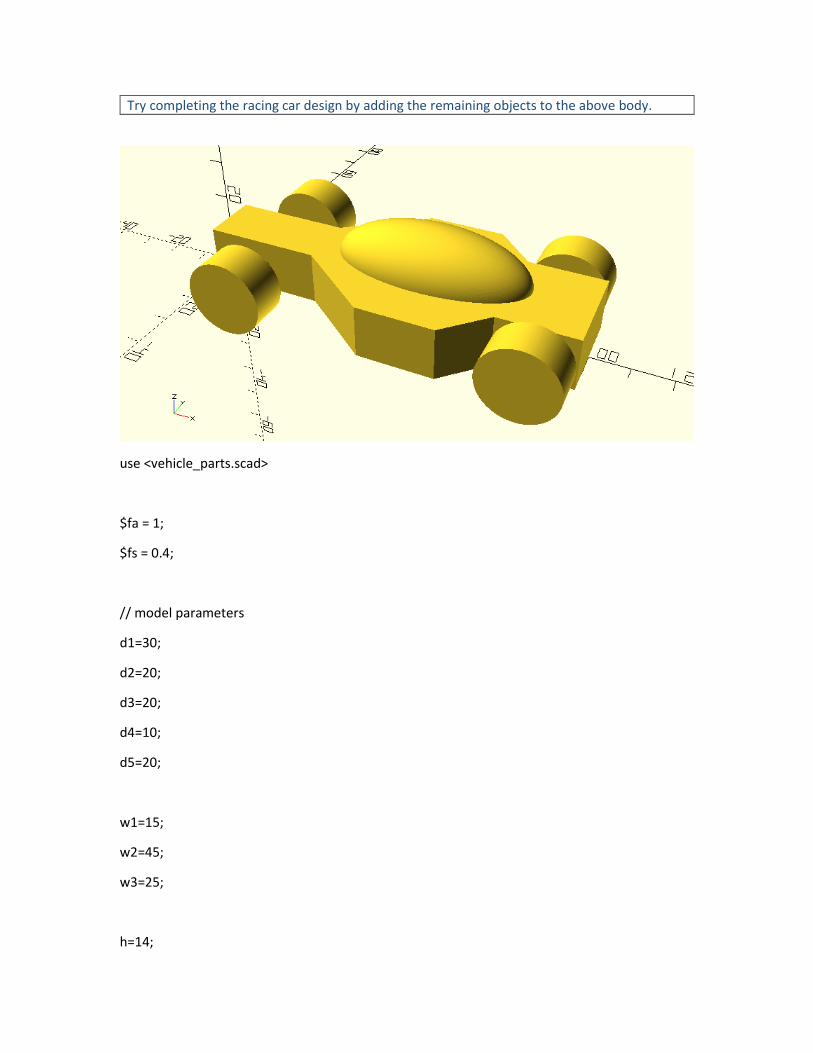
Try completing the racing car design by adding the remaining objects to the above body.


$fa = 1;

$fs = 0.4;

// model parameters

d1=30;

d2=20;

d3=20;

d4=10;

d5=20;

w1=15;

w2=45;

w3=25;

h=14;

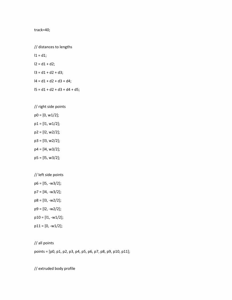
track=40;


l1 = d1;

l2 = d1 + d2;

l3 = d1 + d2 + d3;

l4 = d1 + d2 + d3 + d4;

l5 = d1 + d2 + d3 + d4 + d5;


p0 = [0, w1/2];

p1 = [l1, w1/2];

p2 = [l2, w2/2];

p3 = [l3, w2/2];

p4 = [l4, w3/2];

p5 = [l5, w3/2];

// left side points

p6 = [l5, -w3/2];

p7 = [l4, -w3/2];

p8 = [l3, -w2/2];

p9 = [l2, -w2/2];

p10 = [l1, -w1/2];

p11 = [0, -w1/2];

// all points




// canopy

translate([d1+d2+d3/2,0,h])resize([d2+d3+d4,w2/2,w2/2])sphere(d=w2/2);

// axles

l_front_axle = d1/2;

l_rear_axle = d1 + d2 + d3 + d4 + d5/2;


translate([l_front_axle,0,h/2])axle(track=track);

translate([l_rear_axle,0,h/2])axle(track=track);

// wheels

translate([l_front_axle,half_track,h/2])simple_wheel(wheel_width=10);

translate([l_front_axle,-half_track,h/2])simple_wheel(wheel_width=10);

translate([l_rear_axle,half_track,h/2])simple_wheel(wheel_width=10);

translate([l_rear_axle,-half_track,h/2])simple_wheel(wheel_width=10);

Creating more complex object using the polygon primitive and math

From the above examples it should be quite obvious that the polygon primitive opens the

possibilities to create objects than would hardly be possible by just using the fundamental 2D or

3D primitives. In these examples you created custom 2D profiles by defining the coordinates of

their points according to a given design. To unlock the true power of the polygon command

thought and to create even more complex and impressive designs you have to programmatically

define the points of your profiles using math. This is because defining each point separately is

not scalable to the hundreds of points that are required to design smooth non-square profiles.

One example of this is the following heart. Can you manually define the required points to

create it? There is no way.

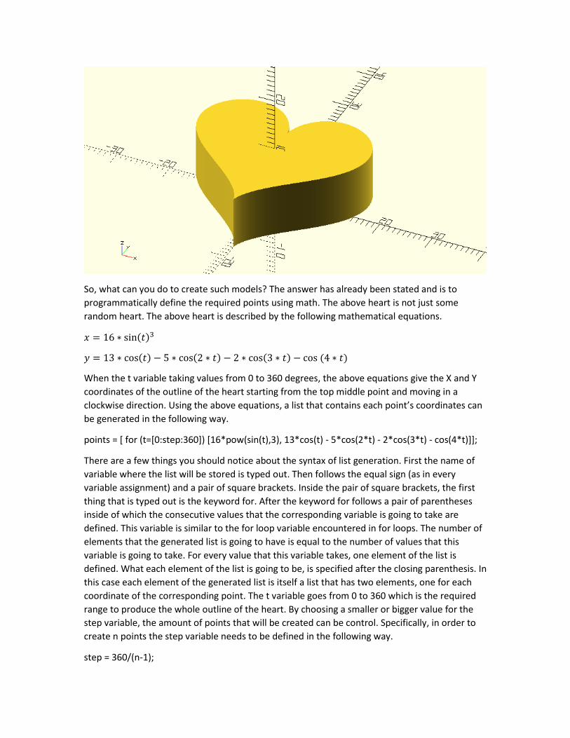
So, what can you do to create such models? The answer has already been stated and is to

programmatically define the required points using math. The above heart is not just some

random heart. The above heart is described by the following mathematical equations.

𝑥 = 16 ∗ sin(𝑡)3

𝑦 = 13 ∗ cos(𝑡) − 5 ∗ cos(2 ∗ 𝑡) − 2 ∗ cos(3 ∗ 𝑡) − cos(4 ∗ 𝑡)

When the t variable taking values from 0 to 360 degrees, the above equations give the X and Y

coordinates of the outline of the heart starting from the top middle point and moving in a

clockwise direction. Using the above equations, a list that contains each point’s coordinates can

be generated in the following way.

points = [ for (t=[0:step:360]) [16*pow(sin(t),3), 13*cos(t) - 5*cos(2*t) - 2*cos(3*t) - cos(4*t)]];

There are a few things you should notice about the syntax of list generation. First the name of

variable where the list will be stored is typed out. Then follows the equal sign (as in every

variable assignment) and a pair of square brackets. Inside the pair of square brackets, the first

thing that is typed out is the keyword for. After the keyword for follows a pair of parentheses

inside of which the consecutive values that the corresponding variable is going to take are

defined. This variable is similar to the for loop variable encountered in for loops. The number of

elements that the generated list is going to have is equal to the number of values that this

variable is going to take. For every value that this variable takes, one element of the list is

defined. What each element of the list is going to be, is specified after the closing parenthesis. In

this case each element of the generated list is itself a list that has two elements, one for each

coordinate of the corresponding point. The t variable goes from 0 to 360 which is the required

range to produce the whole outline of the heart. By choosing a smaller or bigger value for the

step variable, the amount of points that will be created can be control. Specifically, in order to

create n points the step variable needs to be defined in the following way.

step = 360/(n-1);

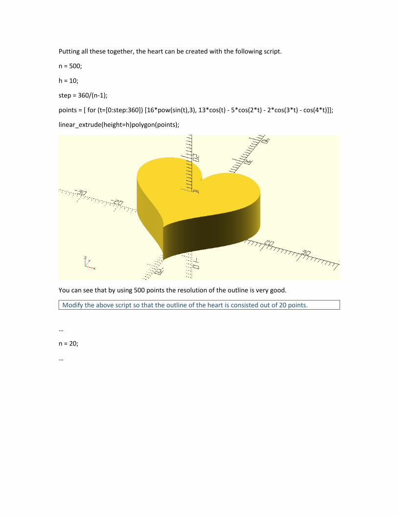
Putting all these together, the heart can be created with the following script.

n = 500;

h = 10;

step = 360/(n-1);

points = [ for (t=[0:step:360]) [16*pow(sin(t),3), 13*cos(t) - 5*cos(2*t) - 2*cos(3*t) - cos(4*t)]];


You can see that by using 500 points the resolution of the outline is very good.

Modify the above script so that the outline of the heart is consisted out of 20 points.

…

n = 20;

…

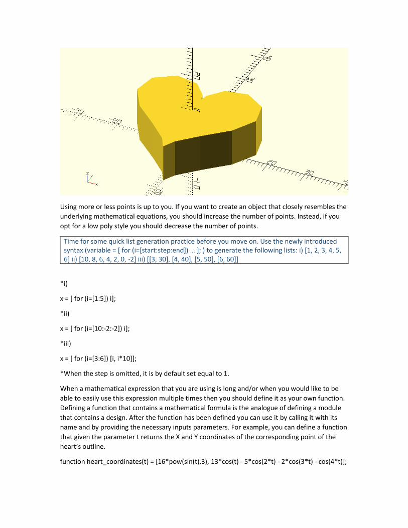
Using more or less points is up to you. If you want to create an object that closely resembles the

underlying mathematical equations, you should increase the number of points. Instead, if you

opt for a low poly style you should decrease the number of points.

Time for some quick list generation practice before you move on. Use the newly introduced syntax (variable = [ for (i=[start:step:end]) … ]; ) to generate the following lists: i) [1, 2, 3, 4, 5, 6] ii) [10, 8, 6, 4, 2, 0, -2] iii) [[3, 30], [4, 40], [5, 50], [6, 60]]

*i)

x = [ for (i=[1:5]) i];

*ii)

x = [ for (i=[10:-2:-2]) i];

*iii)

x = [ for (i=[3:6]) [i, i*10]];

*When the step is omitted, it is by default set equal to 1.

When a mathematical expression that you are using is long and/or when you would like to be

able to easily use this expression multiple times then you should define it as your own function.

Defining a function that contains a mathematical formula is the analogue of defining a module

that contains a design. After the function has been defined you can use it by calling it with its

name and by providing the necessary inputs parameters. For example, you can define a function

that given the parameter t returns the X and Y coordinates of the corresponding point of the

heart’s outline.

function heart_coordinates(t) = [16*pow(sin(t),3), 13*cos(t) - 5*cos(2*t) - 2*cos(3*t) - cos(4*t)];

In this case the script that creates the heart would take the following form.

n = 500;

h = 10;

step = 360/(n-1);


points = [ for (t=[0:step:360]) heart_coordinates(t)];


There are a few things you should notice about the definition of a function. First the word

function is typed out. Then follows the name that you want to give to the function. In this case

the function is named heart_coordinates. After the name of the function follows a pair of

parentheses that contains the input parameters of the function. The input parameters similar to

their use in modules can also have a default value. In this case the only input parameter is the

desired number of points n and it’s not given a default value. After the closing parenthesis

follows the equal sign and the command that defines the pair of X and Y coordinates of the

heart’s outline.

The generation of the list of points can also be turned in a function. This can be done in a similar

fashion as follows.

function heart_points(n=50) = [ for (t=[0:360/(n-1):360]) heart_coordinates(t)];

In this case the script that creates the heart would take the following form.

n=20;

h = 10;


function heart_points(n=50) = [ for (t=[0:360/(n-1):360]) heart_coordinates(t)];

points = heart_points(n=n);


In short you should remember that any command that returns a single value or a list of values

can be turned into a function. Like modules, functions should be used to organize your designs

and make then reusable.

Since you have already defined the function for generating the list of points that is required to create a heart, it would be a good ide to also define a module that creates a heart. Create a module named heart. The module should have two input parameter h and n corresponding to the height of the heart and the number of points used. The module should call the heart_points function to create the required list of points and then pass that list to a polygon

command to create the 2D profile of the heart. This profile should be extruded to the specified height.

module heart(h=10, n=50) {

points = heart_points(n=n);


}

You can save the heart_coordinates and heart_points functions along with the heart module on a script named heart.scad and add it on your libraries. Every time you want to include a heart on a design that you are working on, you can use the use command to make the functions and modules of this script available to you.

Challenge

You are going to put your knew skills into practice to create an aerodynamic spoiler for your

racing car!

You are going to use a symmetrical 4-digit NACA airfoil for your spoiler. The half thickness of

such an airfoil on a given point x is given by the formula 𝑦𝑡 = 5 ∗ 𝑡 ∗ [0.2969 ∗ ξ𝑥 − 0.1260 ∗𝑥 − 0.3516 ∗ 𝑥2 + 0.2843 ∗ 𝑥3 − 0.1015 ∗ 𝑥4]. In the above formula x is the position along the chord with 0 corresponding to the leading edge and 1 to the trailing edge, while t is the maximum thickness of the airfoil expressed as a percentage of the chord. Create a function named naca_half_thickness. The function should have two input parameter, x and t. Given x and t the function should return the half thickness of the corresponding NACA airfoil. The x and t input parameter shouldn’t have any default value.

function naca_half_thickness(x,t) = 5*t*(0.2969*sqrt(x) - 0.1260*x - 0.3516*pow(x,2) +

0.2843*pow(x,3) - 0.1015*pow(x,4));

Create a function named naca_top_coordinates. This function should return a list that contains the pairs of X and Y coordinates for the top half of the airfoil. The first point should correspond to the leading edge while the last point should correspond to the trailing edge. The function should have two input parameter, t and n. The parameter t should correspond to the airfoil’s maximum thickness while the parameter n should correspond to the number of created points. The list of points should be generated using an appropriate list generation command. You will need to call the naca_half_thickness function.

function naca_top_coordinates(t,n) = [ for (x=[0:1/(n-1):1]) [x, naca_half_thickness(x,t)]];

Create a similar function named naca_bottom_coordinates that returns a list of points for the bottom half of the airfoil. This time the points should be given in reverse order. The first point should correspond to the trailing edge while the last point should correspond to the leading edge. This is done so that when the lists that are generated from the naca_top_coordinates and naca_bottom_coordinates functions are joined, all point of the airfoil are defined in a clockwise direction starting from the leading edge, thus making the resulting list suitable for use with the polygon command.

function naca_bottom_coordinates(t,n) = [ for (x=[1:-1/(n-1):0]) [x, - naca_half_thickness(x,t)]];

Create a function named naca_coordinates that joins the two lists of points. To join any number of lists you can use an available command that has this function. This command is called concat. The concat command takes as inputs the to be joined lists.

function naca_coordinates(t,n) = concat(naca_top_coordinates(t,n),

naca_bottom_coordinates(t,n));

Try using the naca_coordinates function to create a list that contains the points for an airfoil with a maximum thickness of 0.12 and with 300 points on each half. The list should be stored in a variable named points. The points variable should be passed to a polygon command to create the airfoils 2D profile.

…

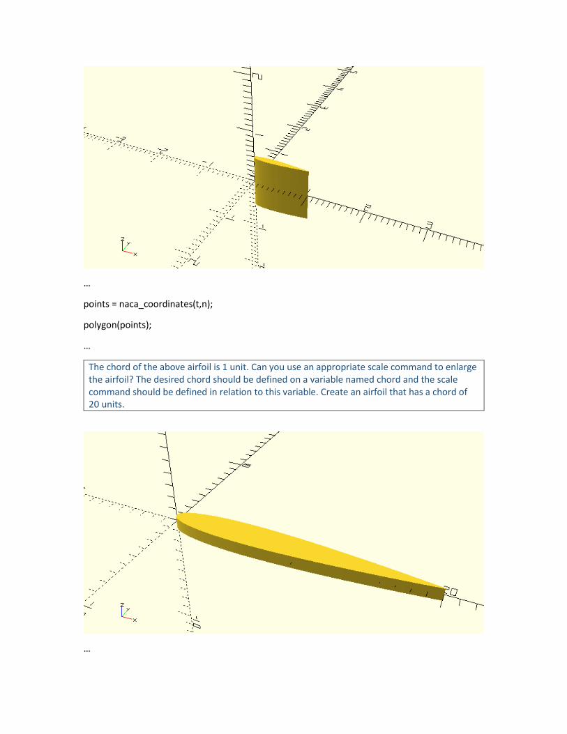
points = naca_coordinates(t,n);

polygon(points);

…

The chord of the above airfoil is 1 unit. Can you use an appropriate scale command to enlarge the airfoil? The desired chord should be defined on a variable named chord and the scale command should be defined in relation to this variable. Create an airfoil that has a chord of 20 units.

…

chord = 20;

points = naca_coordinates(t=0.12,n=300);

scale([chord,chord,1])polygon(points);

…

Turn the above script into a module named naca_airfoil. The module should have three input parameter, chord, t and n. There shouldn’t be default values for any of the input parameters.

module naca_airfoil(chord,t,n) {

points = naca_coordinates(t,n);

scale([chord,chord,1])polygon(points);

}

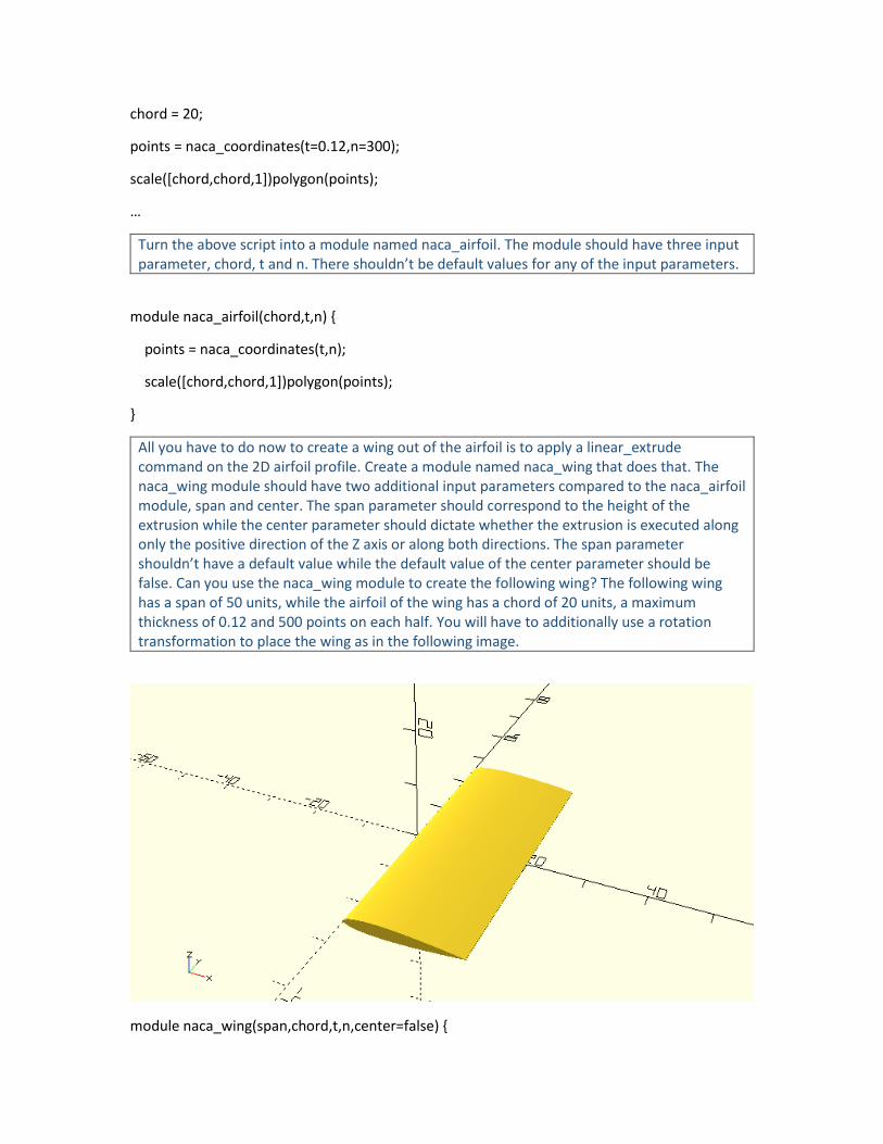
All you have to do now to create a wing out of the airfoil is to apply a linear_extrude command on the 2D airfoil profile. Create a module named naca_wing that does that. The naca_wing module should have two additional input parameters compared to the naca_airfoil module, span and center. The span parameter should correspond to the height of the extrusion while the center parameter should dictate whether the extrusion is executed along only the positive direction of the Z axis or along both directions. The span parameter shouldn’t have a default value while the default value of the center parameter should be false. Can you use the naca_wing module to create the following wing? The following wing has a span of 50 units, while the airfoil of the wing has a chord of 20 units, a maximum thickness of 0.12 and 500 points on each half. You will have to additionally use a rotation transformation to place the wing as in the following image.

module naca_wing(span,chord,t,n,center=false) {

linear_extrude(height=span,center=center) {

naca_airfoil(chord,t,n);

}

}

…

rotate([90,0,0])naca_wing(span=50,chord=20,t=0.12,n=500,center=true);

…

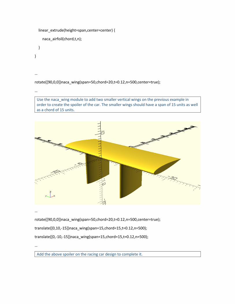
Use the naca_wing module to add two smaller vertical wings on the previous example in order to create the spoiler of the car. The smaller wings should have a span of 15 units as well as a chord of 15 units.

…


translate([0,10,-15])naca_wing(span=15,chord=15,t=0.12,n=500);

translate([0,-10,-15])naca_wing(span=15,chord=15,t=0.12,n=500);

…

Add the above spoiler on the racing car design to complete it.


$fa = 1;

$fs = 0.4;

// model parameters

d1=30;

d2=20;

d3=20;

d4=10;

d5=20;

w1=15;

w2=45;

w3=25;

h=14;

track=40;


l1 = d1;

l2 = d1 + d2;

l3 = d1 + d2 + d3;

l4 = d1 + d2 + d3 + d4;

l5 = d1 + d2 + d3 + d4 + d5;


p0 = [0, w1/2];

p1 = [l1, w1/2];

p2 = [l2, w2/2];

p3 = [l3, w2/2];

p4 = [l4, w3/2];

p5 = [l5, w3/2];

// left side points

p6 = [l5, -w3/2];

p7 = [l4, -w3/2];

p8 = [l3, -w2/2];

p9 = [l2, -w2/2];

p10 = [l1, -w1/2];

p11 = [0, -w1/2];

// all points




// canopy

translate([d1+d2+d3/2,0,h])resize([d2+d3+d4,w2/2,w2/2])sphere(d=w2/2);

// axles

l_front_axle = d1/2;

l_rear_axle = d1 + d2 + d3 + d4 + d5/2;


translate([l_front_axle,0,h/2])axle(track=track);

translate([l_rear_axle,0,h/2])axle(track=track);

// wheels

translate([l_front_axle,half_track,h/2])simple_wheel(wheel_width=10);

translate([l_front_axle,-half_track,h/2])simple_wheel(wheel_width=10);

translate([l_rear_axle,half_track,h/2])simple_wheel(wheel_width=10);

translate([l_rear_axle,-half_track,h/2])simple_wheel(wheel_width=10);

// spoiler

use <naca.scad>

module car_spoiler() {


translate([0,10,-15])naca_wing(span=15,chord=15,t=0.12,n=500);

translate([0,-10,-15])naca_wing(span=15,chord=15,t=0.12,n=500);

}

translate([l4+d5/2,0,25])car_spoiler();

chapter 9files.openscad.org/tutorial/chapter_9.pdf · chapter 9 doing math calculations in openscad...

Documents