chapter iii research methodology chapter -...
TRANSCRIPT

84
CHAPTER III Research Methodology Chapter
3.1. Introduction
Research methodology is a way to systematically solve the research problem. The
purpose of this chapter is to show why this current study has been undertaken, how
the problem has been defined, in what way and why the hypothesizes have been
formulated, what data have been collected and what particular method has been
adopted, and why particular technique of analyzing of data has been used.
The large volume of numerical (quantitative) information gives rise to the need for
systematic methods which can be used to organize, present, analyze, and interpret the
information effectively.
From the 1980s, researchers in developed and developing countries expressed a
renewed interest in information about cash flows. One aspect of that interest focused
on the assertion of the Financial Accounting Standards Board (FASB 1978), which
pointed out that “enterprise earnings based on accrual accounting generally provides a
better indication of an enterprise’s present and continuing ability to generate favorable
cash flows than information limited to cash flows alone.”. This assertion was
questioned, both directly and indirectly, in research that compared the predictive
ability of accrual-based information to that of cash flow information in three different
settings: (1) Bankruptcy prediction, (2) Predicting security returns, and (3) Predicting
operating cash flows.
The cash flow prediction studies ask whether net income (aggregated earnings) alone,
operating cash flow alone or a combination of operating cash flow and accrual
components of earnings is a better predictor of future operating cash flow.

85
They have used single as well as multiple models for showing association between the
cash flows from operation data of each year and the aggregated earnings (earnings
alone), the cash flows from operation (alone), and combination of flows from
operation and components of earnings previous years.
Investors as well as creditors are clearly concerned about a firm’s future cash flows. A
primary objective of financial reporting is to provide information to help investors,
creditors, and others assess the amount, timing and uncertainty of prospective cash
flows. The problem is, however, that prospective cash flows are elusive and difficult
to pinpoint, because the term literally means all prospective flows of cash. A
researcher who wants to find a number that represents .prospective cash flows
encounters many problems.
Prior studies have led to conflicting results. Some research in a single variable testing
model has concluded that the predictive ability of earnings outperforms that of cash
flows in forecasting future cash flows. In contrast, some findings showed conflicting
results in which cash flows are the better predictor of future cash flows. However a
study rejected both conclusions and claimed that neither earnings nor cash flows are a
good predictor of future cash flows.
In addition to single variable testing, some researchers have focused on multiple
variables, such as the components of earnings including cash flow and accrual
accounting data. They concluded that each accrual component reflected different
information relating to future cash flows. In contrast of them a study concluded that
accruals do not improve upon current cash flow in predicting future cash flows.
Moreover, most research has focused narrowly on operating cash flow, earnings and
accrual components of earnings. Those previous studies have ignored the potential of
other cash flow variables, particularly cash flow ratios.
86
Prior studies carried some issues in cases of deriving cash flows from operation in
their models, how comparing predictive accuracy of their models, their time span and
sample size. Also they did not concern about some questions such as whether
predictive ability of the variables are the same across the different industries, and also
whether predictive ability of the variables are different in the indexed companies (
small-cap, mid-cap,…) in compare with no indexed companies. Moreover no study
focused on different predictive accuracy measures to compare their capabilities to test
of hypothesis. In addition the prior studies did not concern about cyclical manners of
models as tools or clue to show turning points of industries or economic conditions.
With purpose of contributing to this field of study, this current work conducted based
on the following questions:
1. Are past earnings significant predictors of future cash flows of Selected Indian
Companies listed on Bombay stock exchange?
2. Are past cash flows significant predictors of future cash flows of Selected Indian
Companies listed on Bombay stock exchange?
3. Are past cash flows and accrual components of earnings significant predictors of
future cash flows of Selected Indian Companies listed on Bombay stock exchange?
4. Are three prediction models, earnings, cash flows and cash flows and accrual
components of earnings models different in predictive powers?
5. Are past cash flow ratios significant predictors of future cash flows of Selected
Indian Companies listed on Bombay stock exchange?
According to the existing conflict on FASB assertion and above research questions
the research hypothesizes have been formulated as bellow:

87
1. (Past) earnings have significant predictive power in estimating future cash
flows of Selected Indian Companies listed on Bombay stock exchange.
2. (Past) cash flows have significant predictive power in estimating future cash
flows of Selected Indian Companies listed on Bombay stock exchange.
3. (Past) cash flows and accrual components of earnings have significant
predictive power in estimating future cash flows of Selected Indian Companies
listed on Bombay stock exchange.
4. Predictions based on three different models do not suggest the same directions
of future cash flows.
5. Ratios calculated based on past cash flows are significant predictors of future
The major purpose of this research is to test hypothesizes. This research intends to test
whether aggregated earnings, cash flows from operation, accrual accounting data, and
cash flow ratios can be used to predict future cash flows of firms by using secondary
data and also evaluate FASB assertion. The models are analyzed to test hypothesizes
and obtain results.
This chapter will continue with following sections as bellow:
In section 3.2, competing researches which already designed to deal with the FASB
assertion have discussed. Selected research design for this study has explained in
section 3.3. Section 3.4 has determined the source of data. Section 3.5 has described
time period of the study. Section 3.6 has shown Sample Selection. Section 3.7 has
explained method of Statistical Analysis, correlation analysis (to check condition to
use the regression technique), procedure to verify of each regression model, analytical
techniques, definition of dependent variable in this study. Section 3.8 has shown
method for conducting regression technique for testing first three hypothesizes.
Section 3.9 has described hypothesis and the models for testing them. Sub-section

88
3.9.1 has shown first hypothesis and related earnings model, independent variable and
measurement in earnings model, and hypothesis testing plan for the first hypothesis.
Sub-section 3.9.2 has shown second hypothesis and related cash flows model,
independent variable and measurement in cash flows model, and hypothesis testing
plan for the second hypothesis. Sub-section 3.9.3 has shown third hypothesis and
related combined model, independent variable and measurement in combined model
hypothesis testing plan for the third hypothesis. Sub-section 3.9.4 has shown forth
hypothesis and evaluation of the predictive ability of the models in and out of sample,
and hypothesis testing plan for the forth hypothesis. Sub-section 3.9.5 fifth hypothesis
and related ratios model, independent variable and measurement in ratios model, and
hypothesis testing plan for the fifth hypothesis. Section 3.10 has explained the validity
of the study, and finally, the conclusion of the chapter is provided in Section 3.11.
3.2. Competing researches which already designed to deal with the
FASB assertion
Apart from bankruptcy investigation, studies on comparative abilities of Accruals
Earnings measures & Cash Flows measures in line of prediction of Future cash flows
Can be categorize in different ways, for instant, they can divided based on how they
have constructed their predictive models, in the case of using dependent variable in
the model they can categorize in two main approaches :
1. The research which examined the comparative abilities of accruals earnings &
cash flows in predicting Securities Prices as a proxy of future cash flows.
2. The studies that compared the accruals earnings measures & cash flows
measures as Predictors of future cash flows from operations (as well as finding
the association between Accruals, future cash flows & future earnings).

89
As the focus of current study was on the second category, it also can be divided in
three main groups in the case of using the independent variables in their models: (1)
Aggregated (earnings) based models; (2) Cash based models, and (3) Combined based
models
In these models independent variables in each model can be from past year (t-1), two
years ago (t-2), and three years ago (t-3) which named as one-year lag, two-year lags,
three-year lags respectively.
These models also can be use in whole (pool) year analysis as well as yearly analysis
of designed hypothesis.
The following figure (figure 2.1) demonstrated the categories in studies related to
cash flows prediction which shows studies on cash flows prediction used different
statistical methods, cross sectional and time series method. In using on cross sectional
method the studies applied pooled cross sectional sample as well as sample which
derived from cross sectional sample by industry.
The studies also have taken different type of data, annuals data as well as quarterly
data in different forms of numbers, absolute, algorithmic, and deflated numbers.
In case of comparing predictive ability of competing models, the researchers have
used in- sample testing alone or together with out- of - sample testing in their studies.
Previous studies also differ from selecting the time span and sample size. The
following figure will show the different aspects of studies on cash flows prediction.

90
Bases of Categorize the studies
Studies on comparative abilities of Accruals Earnings measures & Cash Flows measures in line of prediction of Future cash flows based on how they have constructed their predictive models, in the case of using dependent variable in the model they can categorize in two main approaches :
Based on
Dependent Variable
in the Model
The research which examined the comparative abilities
of accruals earnings & cash flows in predicting
Securities Prices as a proxy of future cash flows.
The studies that compared the accruals earnings measures & cash flows measures as
Predictors of future cash flows from operations
Based on Independent Variables in the Model
Cash based Models
Core Vs.
noncore
Estimated Vs.
Statement
Direct Vs.
Indirect
Cash ratios
Accruals based Models (Aggregated
Earnings)
Mixed based Models (Disaggregated
Earnings)
Accruals
Cash Flows
Short Vs.
Long term
Normal Vs.
Abnormal
Based on Break down of Independent
Variables or
Apply different methods for calculating
Independent Variables
in the Model
Based on Using different
Statistical Methods
Cross Sectional
Pooled Cross Sectional
Cross Sectional By Industry
Firm Specific (Time series)
Based on
Using Different Type of
Accounting Data
Annuals Data
Deflated numbers by average assets or equity
Deflated numbers By inflation indexes
Absolute numbers Algorithmic numbers
Quarterly Data
Comparing Predictive accuracy
Out of sample (MAPE) test
Time span Short horizon Long horizon
Sample size Fewer Firms More Firms
Control for: Size of firms, Life cycle stages, Geographical location, Ownership, & Economic cycle
In sample (using R2) testing
Figure 2.1: Different aspects of studies on cash flows prediction

91
3.3. Selected research design for this study Based on viewing the previous studies; this study chose the design which aim to
contribute in more than two decades working that concentrated on the topic which
compare the abilities of accruals earnings measures and cash flows measures in line of
prediction of Future cash flows by using cash flows from operations (derived from
cash flows statement prepared based on indirect method). In temping to resolve
some lack in some previous studies the current study on cash flows prediction has
following general characters:
3.4. Source of Data
This current study designed to use the annual accounting data of selected Indian
companies listed on Bombay Stock Exchanges which needed in the current study
from Center for Monitoring Indian Economy (CMIE ) data base (14, May,
2009),called “Prowess” which available in Research center of Sinhgad Institute of
management of Pune University in India.
3.5. Time Period of the Study
This study designed to use past year (t-1), two years ago (t-2), and three years ago (t-
3) annual data of independent variable in each model which is named as one-year lag,
two-year lags, three-year lags respectively.
The study selected the time period from 1998 to 2008 as main time span to collect the
data and to complete the year lag data, the annual data 1995 to 1997 also add to main
data. Thus the testing period will be as bellow:

92
Table 3.1: Time period of the study
Year of prediction
One-year lag
(t-1)
Two-year lags
(t-1+t-2)
Three-yearlags
(t-1+t-2+t-3)
1998 1997 1996-1997 1995-1997
1999 1998 1997-1998 1996-1998
2000 1999 1998-1999 1997-1999
2001 2000 1999-2000 1998-2000
2002 2001 2000-2001 1999-2001
2003 2002 2001-2002 2000-2002
2004 2003 2002-2003 2001-2003
2005 2004 2003-2004 2002-2004
2006 2005 2004-2005 2003-2005
2007 2006 2005-2006 2004-2006
2008 2007 2006-2007 2005-2007
3.6. Sample Selection
The study designed to select sample from non financial firms available on CMIE
data base according to following criteria, that means the non financial firms which
satisfy the criteria will be in the sample.
- Availability of cash flow from operation data (as dependent variable) for the firm in
entire main time span (1998 to 2008) for non indexed firm ( indexed firms usually
satisfy this condition but for rare case it will ignore this point for them).
- The firms which their standard value (Z standard) cash flows from operations data
(within the time span) are more than + 2 will exclude from the sample. Outliers will
identify

93
The sample includes 1894 companies listed on the Bombay Stock Exchange between
1998 and 2008 which selected as bellow:
Table 3.2: sample selection procedure
Details
Number
of Firms
Firms listed on BSE on CMIE database 5057
Exclude the financial firms (839)
Exclude the firms which have no cash flow data in entire time span (2270)
Exclude the firms which standard value of their cash flows was more
than + 2
(54)
The firms which satisfy the criteria 1894
Table 3.3: Detail of selected sample
Industry Small cap Mid cap Other index Non Indexed Total
Food & beverages 33 14 3 110 160 Textiles 25 1 175 201 Chemicals 82 41 12 264 399 Nonmetallic Mineral 25 8 1 66 100 Metal & Metal products 36 10 7 100 153 Machinery 56 16 8 151 231 Transport equipment 20 3 2 63 88 Miscellaneous Manufacturing 10 4 - 63 77 Diversified 10 2 1 9 22 Mining 4 3 2 7 16 Electricity 2 4 3 3 12 Services other than finance 91 39 15 189 334 Construction 33 22 5 41 101
Total 427 167 59 1241 1894

94
3.7. Method of Statistical Analysis
The main job of this study was to check the fit of models to predict accurate future
cash flows. The R2 measures the amount to which the models explain or account for
the amount of variability in the dependent variable. To find the more accurate model
in Indian context, based on in-sample comparing test, the R2 is suggested by previous
studies. To derive the R2 of the competing models, running the regression technique is
required.This study has employed the ordinary least squares approaches to estimate
their regression models. To evaluate the forecasting performance of the models, both
within-sample (the R2) and out-of-sample forecasting tests [The mean absolute
percentage errors of prediction (MAPE) , Theil’s U-statistics which used by Kim and Kross
(2005), and Voung's test (Z-statistic) to select the more accurate model based on the
explanation of Dechow (1994) about non nested model selection] are employed.
In a statistical investigation the important concern is to use the right technique for
right data and to answer to right question. To apply right technique, need to check the
condition for that technique. Thus, descriptive statistics (to check rightness of data)
and correlation analysis (to check condition to use the regression technique) are
conducted for this mater.
3.7.1. Correlation analysis (to check condition to use the regression
technique)
If there is no correlation among each dependent and independent variable, the
regression should not be conducted. However, the high correlation among
independent variables indicates the presence of multicollinearity. A measure of the
correlation is represented by correlation coefficients. The coefficient provides both
the direction and strength of the relationship between a pair of variables. In this

95
research, the strength of association between all pairs of variables was statistically
measured by Pearson’s correlation coefficient.
. 3.7.2. Procedure to verify of each regression model
As regression technique has selected for this study, the procedure to verify of each
regression model is as bellow:
1. Are the coefficients significant as a group? (i.e. is the whole model
significant?) => F-test
2. Test for individual regression coefficients
=> t-test (should be performed only if the F-test is significant)
3. How much variation does the regression equation explain?
=> Coefficient of determination (R2)
4. The null hypothesis (H0) to verify is that there is no effect on CFO
The alternative hypothesis (HA) is that this is not the case
H0: α = β = 0
HA: at least one of the coefficients is not zero
Empirical F-value and the appropriate p-value are computed by SPSS. Thus (Sig. <
0.05), we can reject H0 in favor of HA. This means that the model that has been
estimated is not only a theoretical construct, but exists and is statistically significant.
3.7.3. Analytical techniques This study has employed the ordinary least squares approaches to estimate their
regression models. To evaluate the forecasting performance of the regression models,
both within-sample and out-of-sample forecasting tests are employed.

96
This research utilized quantitative methods in which the data is analyzed based on
statistical techniques, which include descriptive statistics, Pearson’s correlation and
regression analysis.
The descriptive statistics provide an initial summary data of the essential features of
the sample. The correlation analysis is used to fundamentally examine the relationship
between dependent and independent variables. Regression analysis, simple linear,
multiple, and stepwise regressions, are applied to test the prediction models
depending upon the ability of predictor variables to explain future cash flows. All
analytical techniques use the computer software package Statistical Processing for
Social Scientists (SPSS) Version 11.5.
3.7.4. Definition of dependent variable in this study
Prior studies could be divided in two groups based on how the studies derived the
cash flow from operation variable in their works. First group contains those studies
which did not use the cash flows statement for derived the cash flow from operation
in their works, such as the studies of Bowen, Burstahler and Daley (1986 in USA);
Greenberg, Johnson & Ramesh (1986 in USA); Espahaodi (1988 in USA); Murdoch
and Krause (1989 in USA); Arnold and et al (1991 in UK); Percy and Stokes (1992
in Australia); Finger (1994 in USA).
The rest of the studies such as McBeth (1993 in US);; Seng (1997 in New Zealand);
Kim and Kross (2005 in USA); Zhao and et al (2006 in Australia); Farshadfar and et
al (2008 in Australia), and Lorek and Willinger (2009 in USA)have used the cash
flows statement for derived the cash flow from operation in their works.
In the analysis, Future cash flows are investigated as the dependent or criterion
variable caused by independent variables.

97
Future cash flows of firms are defined as net cash flows from operations (CFO)
reported in cash flow statements for the year t, represented by the symbol of CFO t.
under the indirect method form and reported by adjusting earnings for non-cash items
and for changes in current assets and current liabilities.
3.8. Method for conducting regression technique for testing first
three hypothesizes.
Simple and multiple regression models were performed between cash flow from
operations year t, CFO t as the dependent variable and year lags of the independent
variables in each model.
For three models the analysis conducted as bellow
Figure 3.1: Summary of conduced analysis for first three hypothesizes
In pooled-year analysis, all data for dependent and independent variables of the ten
years prediction period of 1998 to 2007 was pooled and analyzed together.
For the yearly analysis, the regression model was processed to analyze each set of
prediction years separately. The analysis was performed for eleven prediction years
spanning 1998 to 2008. In each prediction year, three sets of data were analyzed
including a set of the one-, two- and three year lags of earnings.
Analysis for hypothesis
Analysis based on whole (pool) sample
Index wise analysis Industrial wise analysis
Pooled year
analysis
Yearly analysis
Pooled year analysis
Yearly analysis
Pooled year analysis
Yearly analysis

98
This study designed to test the research hypothesis based on character of the firms
share (stock) in Bombay Stock Exchanges (BSE) which demonstrated by CMIE data
base as bellow:
- BSE small-cap (non financial cases)
- BSE mid-cap (non financial cases)
- Other share in BSE 500 which are not small-cap or mid-cap (non financial cases )
- Non indexed firms (which are not included in the above indexes)
This study also designed to test the research hypothesis (earnings model, cash flows
model, combined model, and ratios model) in a whole (pool) sample which contained
varieties of firm from spectrum of industries listed on Bombay Stock Exchanges
(BSE) as well as a cross sectional sample which divide base on different sectors of
industries that allows to compare the abilities of independent variables in different
industry which will give us a detail picture about cash flows prediction possibility and
importance of accounting figures in each industry.
This study designed to test the research hypothesis in whole (pool) sample and cross
sectional sample by industry in two different bases: pooled-year based, yearly based
as well.

99
3.9. Hypothesis and the models for testing them 3.9.1. First hypothesis and related earnings model Past earnings have significant predictive power in estimating future cash flows of
Selected Indian Companies listed on Bombay stock exchange.
Table 3.4: Models for first hypothesis
HYPO Models Regression equation
Type of
regression
Earnings models
# 1
One-year
lag CFOn,t = α0 + β1 EARNn,t-1 + ε Simple
Two-year
lags
CFOn,t = α0 + β1 EARNn, t-1 + β 2
EARNi, t-2 + ε Multiple
Three-year
lags
CFOn,t = α0 + β1 EARNn, t-1 + β 2
EARNi, t-2 + β 3 EARNi, t-3 + ε Multiple
Independent variable and measurement in earnings model Net income before extraordinary items and discontinued operations derived from
income statements for the previous years is used as the measure of past earnings
Earnings of firms are defined as net income before extraordinary items and
discontinued operations reported on income statements for year t-i symbolized by
EARNt-i.
100
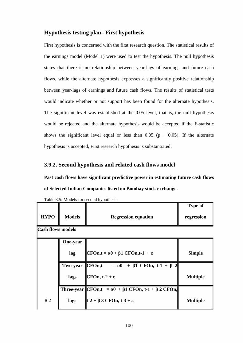
Hypothesis testing plan– First hypothesis First hypothesis is concerned with the first research question. The statistical results of
the earnings model (Model 1) were used to test the hypothesis. The null hypothesis
states that there is no relationship between year-lags of earnings and future cash
flows, while the alternate hypothesis expresses a significantly positive relationship
between year-lags of earnings and future cash flows. The results of statistical tests
would indicate whether or not support has been found for the alternate hypothesis.
The significant level was established at the 0.05 level, that is, the null hypothesis
would be rejected and the alternate hypothesis would be accepted if the F-statistic
shows the significant level equal or less than 0.05 (p _ 0.05). If the alternate
hypothesis is accepted, First research hypothesis is substantiated.
3.9.2. Second hypothesis and related cash flows model Past cash flows have significant predictive power in estimating future cash flows
of Selected Indian Companies listed on Bombay stock exchange.
Table 3.5: Models for second hypothesis
HYPO Models Regression equation
Type of
regression
Cash flows models
# 2
One-year
lag CFOn,t = α0 + β1 CFOn,t-1 + ε Simple
Two-year
lags
CFOn,t = α0 + β1 CFOn, t-1 + β 2
CFOn, t-2 + ε Multiple
Three-year
lags
CFOn,t = α0 + β1 CFOn, t-1 + β 2 CFOn,
t-2 + β 3 CFOn, t-3 + ε Multiple

101
Independent variable and measurement in cash flows model The definition of past cash flow variable is net cash flow reported on statements of
cash flows for the previous years.
Cash flow is defined as net cash flows from operations reported on the cash flow
statements for year t-i, denoted by CFOt-i.
Hypothesis testing plan – Second hypothesis Second hypothesis is concerned with the second research question. The null
hypothesis states that there is no relationship between year-lags of cash flows and
future cash flows while; the alternate hypothesis expresses a significantly positive
relationship between year-lags of cash flows and future cash flows. Similarly to the
earnings model, the significant level was established at the 0.05 level. The null
hypothesis would be rejected and the alternate hypothesis would be accepted if the F
test of the cash flows model (Model 2) show that the variance in future cash flows has
been significantly explained by the year-lags of cash flows at the significant level
equal or less than 0.05 (p _ 0.05). If the alternate hypothesis is accepted, second
research hypothesis is substantiated.

102
3.9.3. Third hypothesis and related combined model Past cash flows and accrual components of earnings have significant predictive power in estimating future cash flows of Selected Indian Companies listed on Bombay stock exchange. Table 3.6: Models for third hypothesis
HYPO Models Regression equation
Type of
regression
Mixed models
# 3
One-year
lag
CFOn,t = α0 + β1 CFOn,t-1 + β 2 ACCn,t-
1 + ε Simple
Two-year
lags
CFOn,t = α0 + β1 CFOn, t-1 + β 2
ACCn,t-1 + β3CFOn, t-2 +
β 4 ACCn,t-2 + ε Multiple
Three-year
lags
CFOn,t = α0 + β1 CFOn, t-1 + β 2
ACCn,t-1 + β3CFOn, t-2 +
β 4 ACCn,t-2 + β5CFOn, t-3 + β 6
ACCn,t-3 + ε Multiple
Independent variable and measurement in combined model The accrual components of earnings are obtained from cash flow statements for the
previous years. Earnings can be disaggregated into cash flow and the component of
accruals. Accrual component include: change in accounts receivable; change in
accounts payable; change in inventory; change in other short-term assets and
liabilities and depreciation and amortization.

103
CFO = EARN-ACC
ACC = EARN-CFO
or
ACC = ∆ AR + ∆ INV + ∆ AP+ DEP + ∆ OTH
Whereas,
∆ AR = Change in accounts receivable during the period
∆ INV = Change in inventories during the period
∆ AP = Change in accounts payable during the period
DEP = Depreciation and amortization during the period
∆ OTH = Change in other current assets and liabilities during the period
This research investigated the predictive ability of the aggregated accrual components
of earnings for the year lags (t-i), was denoted as ACC,t-i.
Hypothesis testing plan – Third hypothesis Third hypothesis is concerned with the third research question. The null hypothesis
states that there is no relationship between cash flows and accrual components of
earnings and future cash flows, while the alternate hypothesis expresses a significant
relationship between year-lags of cash flows and accrual components of earnings and
future cash flows. The null hypothesis would be rejected and the alternate hypothesis
would be accepted if the F-statistic of cash flows and accrual components of earnings
model (Model 3) shows the significant level equal or less than 0.05 (p _ 0.05). Third
research hypothesis is substantiated when the alternate hypothesis is accepted.

104
3.9.4. Forth hypothesis and evaluation of the predictive ability of the models in and out of sample.
Predictions based on three different models do not suggest the same directions of
future cash flows.
This study designed to test the forth hypothesis, comparing predictive ability of
competing models (first, second, and third hypothesis) by using In-sample and Out-
of-sample tests which it requires to do following procedures in each test.
1. In-Sample test for comparing predictive ability of competing models
The adjusted R2 value has been employed by previous prediction research to evaluate
the explanatory power between models, such as Barth, Cram and Nelson (2001),
Quirin et al (1999), Greenberg, Johnson and Ramesh (1986), and McBeth (1993). The
model producing a high adjusted R2 value is a good explanatory model and it can be
an important predictive model.
2. Out-Of-Sample test for comparing predictive ability of competing models
In addition to adjusted R2, current study employed the analysis of residuals involving
the mean absolute percentage error to evaluate the predictive abilities of the prediction
models.
The mean absolute errors generate from the out-of sample period. That is, the sample
split into two parts. The first sample, the estimated sample, to create regression
equations of each prediction model and the second sample, the-out-of sample, to test
the estimated equation of the three models; earnings, cash flows and cash flows and
accrual components of earnings models (first, second, and third hypothesis).
After calculating the predicted values of cash flows from the out-of sample, the r
square (r2), mean absolute percentage errors of prediction (MAPE) and Theil’s U-
statistics used by Kim and Kross (2005) calculate for the out-of-sample period. A

105
model producing relatively low MAPE would be considered to be a better predictor
than model yielding higher MAPE. The MAPE is calculated as below:
MAPE = mean | (actual – predicted) / actual |
The U statistic can range from zero to one, with zero implying a perfect forecast.
Thus, models generating better predictions should have lower U statistics. Theil’s U is
defined as the square root of
Σ (actual – predicted) 2 / Σ (actual) 2.
To calculate the statistic for doing out-of-sample test the original sample (1998 to
2008) will split into two parts:
1. 1998 to 2005: to create regression equations of each prediction model
2. 2006 to 2008: to test the estimated equation of the three models;
earnings, cash flows and cash flows and accrual components of
earnings models (first, second, and third hypothesis).
Based on explanation of Dechow (1994) about non nested model selection, in out-o-
sample testing, this study also applied Voung's test (Z-statistic) to select the more
accurate model. The formulas are as bellow

106
Hypothesis testing plan – Forth hypothesis Forth hypothesis intends to answer forth research question. Adjusted R2 values,
correlations between actual and predicted cash flows, and mean absolute percentage
errors of each model were used to evaluate the predictive ability of each model. The
comparisons of these values were used to test the hypotheses.
3.9.5. Fifth hypothesis and related ratios model Ratio based analysis of past cash flows is significant predictor of future cash
flows of Selected Indian Companies listed on Bombay stock exchange. Table 3.7: Models for fifth hypothesis
HYPO Models Regression equation
Type of
regression
Ratios model
# 5
One-year
lag CFOn,t = α0 + β1 ∑ i=1 to10 CFR t-1 + ε
stepwise
procedure
Since there were many cash flow ratios considered to be predictors in the model,
variable selection technique was used to choose which cash flow ratios are important.
Stepwise regression was selected to examine each cash flow ratio. Each predictor
variable is considered for addition prior to developing the regression equation. In the
procedure, each possible predictor variable in simple regression was examined. Then
the explanatory variable providing the largest partial F statistic was chosen to add to
the model. Finally, the stepwise procedure generated suitable equations for the model.

107
Independent variable and measurement in ratios model 1) Cash flow sufficiency ratios Cash flow sufficiency ratios are aimed at assessing a company’s relative ability to
generate sufficient cash to meet its cash flow needs. All ratios indicate whether a
company’s cash flows are sufficient for the payment of debt, acquisitions of assets
and payment of dividends. These ratios are cash flow adequacy, debt coverage, and
repayment of borrowing and dividend payment ratios.
• Cash flow adequacy ratio
The cash flow adequacy ratio is an attempt to assess the entity’s ability to produce
sufficient operating cash flows to cover its main cash requirement, specifically, the
payment of debt, the acquisition of assets, and the payment of dividends.
• Debt coverage ratio
The debt coverage ratio shows the ability of a company to generate cash flow from
operating activities to pay its long-term debt commitment.
• Repayment of borrowings ratio
This ratio indicates the ability of a firm to generate cash from operating activities for
the purpose of covering long-term debt commitments in the current year.
• Dividend payment ratio
The dividend payment ratio presents the ability of a company to generate cash from
operating activities for the purpose of covering dividend commitments to both

108
ordinary and preference shareholders. If the ratio is greater, it means that the company
paid a smaller portion of its cash from operating activities in dividend payments.
• Reinvestment ratio
The reinvestment ratio presents the ability of a company to generate cash from
operating activities for the purpose of covering asset acquisition payments.
2) Cash flow returns ratios This group is sometimes called efficiency ratios. It shows the ability of a company to
generate operating cash flows. Cash flow efficiency ratios are used to assess the
relationship between items in the income statement and balance sheet with cash flow
from operations as disclosed in the cash flow statement. These ratios are as follows.
• Cash flow on revenues ratio
This ratio is aimed at showing the ability of the company to turn revenue into cash.
The higher ratio is the better the ability. This ratio employs information provided by
the statement of cash flow and the income statement. It is computed by dividing cash
from operating activities by revenues.
• Cash flow to net income ratio
This ratio is sometimes called the operating index. It compares the company’s profit
with cash flow from operations and attempts to provide an index of the cash-
generating productivity of operations. It is calculated as cash flows from operations
divided by profit after income tax.

109
• Cash flow return on assets ratio
This ratio attempts to measure the company’s return on assets in term of the cash flow
generated from operations.
• Cash flow return on stockholders’ equity ratio
This ratio shows the ability of the company to generate a sufficient cash return for
stockholders.
• Cash flow per share ratio
This ratio indicates the operating cash flow attributable to each common share. It is
defined as cash available to common stockholders divided by the weighted average
number of common shares outstanding.

110
Hypothesis testing plan – Fifth hypothesis This hypothesis involves testing the predictive power of cash flows ratios in
predicting future cash flows. The null hypothesis states that the cash flow ratios do
not provide a good predictor for predicting future cash flows of Indian listed
companies. In other words, the alternate hypothesis states that cash flow ratios
provide a good predictor for predicting future cash flows of Indian listed companies.
The results of the stepwise analysis were used to test the hypothesis.
3.10. The validity of the study External validity refers to the extent to which the result of a study may be generalized
to other samples. Accounting data used in this study are historical which may have
caused a low level of external validity. That is, the result of a particular study at a
point in time may not be generalized to other periods of time. In the analysis, this
study attempted to eliminate this disadvantage by using data for many years which
cover a period from 1998 to 2008.Data of each year were analyzed separately to
observe whether the economic condition caused a different result.
3.11. Conclusion on Research Methodology Chapter This chapter provided the methodology used in this study including FASB assertion
and its influence to develop competing hypothesis, competing research design to
approve the FASB assertion, properties of the research design which chose the
(operating) cash flows data as a dependent variable in their study, source of data, time
period of the study, sample selection, method of statistical analysis, testing predictive
accuracy, analytical techniques, definition of dependent variable in this study,
hypothesis and the models for testing them. This research deals with testing
hypotheses and chiefly focuses on quantitative methods. The basic method used to

111
collect data was the use of secondary data, which suited the data needs in this
research. That is, accounting data reported on financial statements of firms were
selected to measure variables.
Additionally, the measurement of variables was defined to test the four prediction
models of this research. The four prediction models consisted of earnings, cash flows,
cash flows and accrual components of earnings and cash flow ratios models. These
models were tested by regression analysis. The study was designed to use an adjusted
R2 reflecting the explanatory power of the model in comparing regression models.
Furthermore, the study planned to evaluate the predictive power of the models by
using a mean of absolute percentage errors and Theil’s U-statistics used by Kim and
Kross (2005) generated from the sample data. Moreover, based on explanation of
Dechow (1994) about non nested model selection, in out-o-sample testing, this study
also applied Voung's test ( Z-statistic) to select the more accurate model.
Finally, the validity issue of the research was discussed in support of the research
design, which reduces the possible low level of external validity of the research. In the
next chapter, the data analysis and results of the analysis are provided.