1

CHAPTER ONE

INTRODUCTION AND LITERATURE REVIEW

1.1 Introduction

Biometrics is the study of methods for measuring physical or behavioral traits of an

individual that can be used for uniquely recognizing or verifying that individual‟s

identity [1]. Physical biometrics based on face recognition, eye print, finger print, and

voice recognition are common as they are easier to measure than behavioral

characteristics such as handwriting and printing type.

The research‟s on biometrics are taking a lot of interest from researchers and

scientists due to its high importance in security and safety systems and the increasing

needs for more and more secure and easy recognition methods. The use of cards with

long difficult passwords represent a big challenge for a lot of people who face

difficulties in remembering their bank accounts, credit cards, even there own

computers passwords. The revolution which happened in the digital technology has

encouraged researchers to make advanced steps in biometrics. The day life use of

digital recognition systems based on biometrics became a reality.

Biometrics are divided into two distinct methods, these are physical methods like face

and eye, and behavioral methods like printing type or walk rhythm. Applications for

biometrics are most common in security, medical, and robotics areas related to

fingerprint, face, iris, and gait. These biometric areas have gained the most attention

among the research community.

The potential for using the ear‟s appearance as a means of personal identification was

recognized and advocated as early as 1890 by the French criminologist Alphonse

Bertillon [1]. Ear recognition has been mentioned and used recently in many

researches. The interest in ear as a physical feature of human is due to its stability

over the years. The ear of a human remain same for the duree of the life with no

important changes. Ear images can be acquired in a similar manner to face images,

and a number of researchers have suggested that the human ear is unique enough to

each individual to allow practical use as a biometric [2]. Many researchers have used

the two dimension ear recognition, other used 3D recognition for ear features. In fact,

2

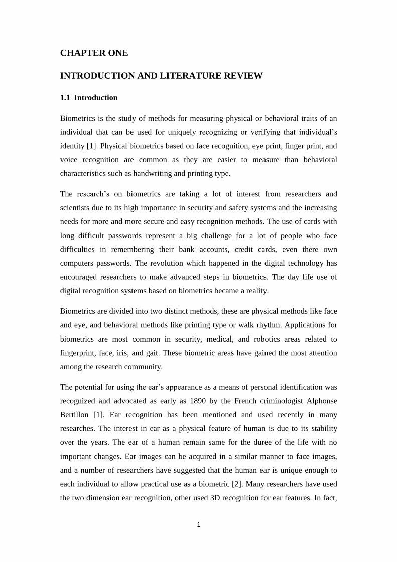
the ear may already be used informally as a biometric. For example, the United States

Immigration and Naturalization Service (INS) has a form giving specifications for the

photograph that indicate that the right ear should be visible (figure 1.1) [2].

Figure 1.1 : INS Form-378 (6-92) Asking for the Right Ear to be Visible [2]

The ear biometric problem (as with all biometrics) is split between enrolment and

recognition. Enrolment is the discovery, localization and normalization of the ear

image, whilst recognition deals with identification of a subject by ears. Currently,

most enrolment for experiments is done manually, but in any real world test of ear

biometrics, enrolment is just as important a problem as recognition. Enrolment has not

seen the same amount of research as recognition but there is some development in the

area [3].

Artificial neural networks has become very famous and applied in many aspects of

science. It is using mathematical equations and formulas to simulate the function and

structure of the brain. Artificial neural networks and back propagation algorithm have

been used widely in biometrics. The use of artificial neural network in face and iris in

addition to fingerprint recognition has been introduced in many researches. Neural

networks are massively parallel computing systems consisting of a large number of

simple processors with many interconnections.

3

The principle of ANN is applied for approximating a function where they learn a

function by looking at examples of this function. Here the internal weights in the

ANN are slowly adjusted so as to produce the same output as in the examples.

Performance is improved over time by iteratively updating the weights in the network.

The hope is that when the ANN is shown a new set of input variables, it will give a

correct output [4]. The training of ANN to perform a task implies the use of sets of

inputs and targets. These sets are considered as examples for teaching the networks.

The internal connections of the network are modified iteratively until finding the

optimum values that approximate the best our input output relationship.

This thesis discusses the use of artificial neural networks in biometric systems. The

ear recognition has been specifically chosen to be performed using back propagation

neural networks. Ear pictures of 54 persons will be used in normal and noisy sets for

the training of ANN.

1.2 Literature Review

The use of ear has been introduced and mentioned since a long time. Many different

extraction and recognition methods have been mentioned and used in literature using

ear characteristics. Researchers are still discussing weather ear is unique or unique

enough to be used in biometrics. The use of ANN for ear recognition has been

introduced in [5]. The basics of using ear as biometric for person identification and

authentication are presented. In [6] a 3D image recognition based on special analysis

has been discussed. A ray transform has been used for ear image recognition in [3].

The use of ear biometrics for person identification based on geometrical structure has

been discussed in [7]. A novel ear enrolment technique using the image ray transform,

based upon an analogy to light rays. The transform is capable of highlighting tubular

structures such as the helix of the ear and spectacle frames and, by exploiting the

elliptical shape of the helix, can be used as the basis of a method for enrolment for ear

biometrics. A review of biometrics and ear recognition techniques has been discussed

in [8]. In [2] and [9] different 2D and 3D images processing techniques for ear

recognition has been discussed. The geometrical structures observed from pixel value

distances are used for the successful recognition of objects.

Spatial segmentation of 2D ear images for recognition purpose has been introduced in

[1]. The author in [10] proposed a geometric approach for ear recognition. A simple

4

two stage scale and rotation invariant geometric approach based on the concept of

maximum line was used. The use of wavelet transform based approach for ear

recognition has been introduced in [11]. A new banana wavelet transform was used

and its performance was compared with Gabor wavelet for ear recognition. an

experimental study to investigate the effect of time difference between image

acquisition for gallery and probe on the performance of ear recognition was also

carried out in this work. A study of computerized ear recognition methods has been

carried out in [12] and [13]. A discussion about ear recognition has been introduced in

[14]. Evaluation of ear recognition has been presented in [15] and [16]. A survey

about image features extractions for ear recognition has been applied by [17].

Biometric recognition using 3D ear shape was discussed in [18]. In [19], a multimodal

biometrics based on face and ear recognition has been discussed.

In [20], the authors discussed a new multi modal biometrics based on face and ear.

The research significance of multi-modal biometrics based on face and ear was

represented, Then some researchers‟ achievements and inadequacies. Different

researches and explorations were done in the paper. A new novel ear enrolment

technique using the image ray transform, based upon an analogy to light rays in [21].

The transform is capable of highlighting tubular structures such as the helix of the ear

and spectacle frames and, by exploiting the elliptical shape of the helix, can be used

as the basis of a method for enrolment for ear biometrics. The presented technique

achieved good results of success. Multimodal biometrics based on fingerprint and ear

biometrics for personal identification was presented in [22]. A novel technique of

edge interaction point detection (EIPD) was used to determine the ear features.

Fingerprint features are identified by line based connected component analysis and its

feature vectors are generated using EIPD system. Also, Neural network based back

propagation network is used for an identity verification system.

An experimental study to demonstrate the effect of the time difference in image

acquisition for gallery and probe on the performance of ear recognition was presented

in [23]. [24] Presented an online biometric authentication using ear contours acquired

from a robust peg free acquisition set up. Gaussian classifiers were used to first

segment the skin and non-skin areas in the ear images. Laplacian of Gaussian was

then used to compute edges of the skin areas; which helped to get ear images. A pixel

based feature extraction for ear biometrics method was proposed by [25].

5

Many other references has discussed the use of ear recognition for person

identification and/or person identity check using different methods. The use of neural

network for identification purpose has been proposed recently in many works. Its

simple structure and high performance in addition to its ease of use compared to the

other methods that need a lot of manual processing have put it in the first of

recognition methods. The work in this thesis proposes the use of ANNs for ear

biometrics based person identification.

6

CHAPTER TWO

BIOMETRICS

2.1 Overview

Confirming the identity of a person nowadays became a very important challenge

facing the society. There exist many identification methods which vary between high

secure and less secure methods. However, some applications and life fields impress

more need for highly secured identification such as military, health, police and banks.

Biometrics has been mentioned as one of the most accurate and secure identification

methods which are being given more and more attention by researchers in the field.

In the traditional classic identification methods, person is to memorize huge

combinations of letters and numbers in order to have access to some places or

applications. Unless these pass-codes or pass-words are correct, people can‟t have

instant access to their works or money.

According to Nilson report, in 2005, MasterCard, Visa, American Express and

Discover incurred US$ 1.14 billion in fraud losses. Also 20 to 50% of helpdesk calls

were for password resets and each password reset costs about US$70. Over more, in

2005, 9.3 million American citizens suffered from identity theft which costs a total of

US$ 54.4 billion [21].

The need for memorizing long pass-phrases and the possibility of these phrases to be

forgotten or even stolen encouraged the researchers more and more toward finding

easier, simple, and more secure identification methods. One of the most secure

methods of identification is biometrics.

Biometrics is the science that studies the behavior exhibited and physical properties in

order to be able to distinguish between people. It represents the study of automated

and semi-automated systems or methods for recognizing a person based on his

physical or behavioral characteristics. Biometrics can be divided into two categories,

identification systems and verification systems. Identification system tells “who are

you”, while verification system tell “are you the person you are claiming yourself to

be?” [10].

7

Biometrics has been used long time ago in the identification of persons; people in the

desert were using the physical and biological signs in the verification of a person

identity. Finger prints and signature has been used for long time as a verification

method hundreds of years ago. The development of science and digital world has

increased the ability of injecting these biometrics and others easily in all fields of the

life. Nowadays fingerprint identity recognition machines and voice recognition

machines are widely used even in very small workplaces.

Memory and token identification methods are implemented to judge if the specified

user should have an access to a specified resource. Therefore an exact identification of

a person is not necessary and indeed is not always performed. It is possible that a

group of people has the same token or know the same password. Biometric

identification methods start with proper identification of a person and only after that,

the proper rights are assigned. Thus the main difference between classic methods and

biometrics is that biometric properties cannot be „borrowed‟ so people cannot - in the

way as simple as giving a token or telling the password - propagate their rights to

others. It obviously increases security of the system but sometimes may cause

problem[22].

First stage in each biometric process is collecting a set of „samples‟ from every user

who should be identified by the system. A sample is a set of biometric data measured

for a person in a single measurement. The biometric data may be a different kind of

psycho-physiological measurements. Next stage in most methods is creating a

„template‟ for each user based on previously collected samples. A template is a kind

of mean from all samples collected for this user. The process of creating a template is

called an „enrolment‟ of the user.

2.2 Characteristics of biometrics

In the opinion of [22 and 23] any human physiological or behavioral characteristic

could be a biometrics just if it has the following desirable properties:

1- Universality, which means that every person should have the

characteristic, if some people doesn‟t have that property then it can‟t be

considered as biometrics.

8

2- Uniqueness, which indicates that no two persons should be the same in

terms of the characteristic, otherwise.

3- Permanence, which means that the characteristic should be invariant with

time.

4- Collectability, which indicates that the characteristic can be measured

quantitatively.

The author in[14] also has mentioned three other conditions which must be achieved

in order to consider a property as to be biometrics, these conditions are:

1- Performance, which refers to the achievable identification accuracy, the

resource requirements to achieve acceptable identification accuracy, and the

working or environmental factors that affect the identification accuracy.

2- Acceptability, which indicates to what extent people are willing to accept the

biometric system.

3- Circumvention, which refers to how easy it is to fool the system by fraudulent

techniques

A biometric feature is a specific attribute of a person that can be measured with some

precision. There are a lot of different biometric features that can be measured[22].

2.3 Evaluation of biometric identification

Measurement of biological quantities is always to some degree imprecise and

therefore is producing different values for the same quantity measured. These errors

are an instant part of every biometric method and the main problem of that kind of

identification is to elaborate algorithms that sufficiently deal with these imprecise

data.

There are two kinds of tests when considering authorization (two class) system:

• Genuine test – when a sample is given with correct identification

information (login). In another words „the identified person is telling the

truth‟. In such case the rate of improper rejections may be measured. This

9

measure is often called a False Rejection Rate (FRR) or False Non-Match

Rate.

• Impostor test – when a sample is given with incorrect login. In another

words „the identified person is lying‟. Now a rate of improper acceptances

may be measured. This measure is called a False Acceptance Rate (FAR) or

False Match Rate [22].

The comparison between the two measures seems to be a good approach in order to

evaluate the identification method. However, still the two measures are related to each

other and decreasing one of them will increase the other.

2.4 Different Biometrics Methods

Most of human body parts has been used or can be used as biometrics, that due to the

fact that the features of each person‟s parts are unique and can‟t be found in the other

persons‟ bodies. The biometrics is divided into two types: the first uses the measure of

fingerprint, iris, eye retina, face, palm teeth, ear, and even smell for some measures.

The second uses the measure of humans‟ behavior patterns such as his way of

speaking, walking, shape of signature, and the hand writing.

Though behavior biometrics is less expensive and less dangerous for the user, physic-

logical characteristics offer highly exact identification of a person. Nevertheless, all

two types provide high level of identification than passwords and cards.

2.5 Physiological types of biometrics

Physiological systems are considered to be more reliable as individual features of a

person, that are used by these systems, do not change by influence of psycho-

emotional state.

2.5.1 Finger Print

Fingerprints are considered being one of the oldest and popular among other bio-

metric technologies. First uses of fingerprints instead of signatures were reported in

19th century. The milestone was adopting a Galton/Henry system of identification by

10

Scotland Yard in 1900. Since then fingerprints became one of the most important

features used in forensic prosecutions [22].

Fingerprint identification is also known as dactyloskopy or also hand identification is

the process of comparing two examples of friction ridge skin impression from human

fingers, palm or toes[24].

There are a lot of easy to use and cheap fingerprint scanners. They are based on

different technologies including optic, capacitive, ultrasound, pressure, thermal and

electric field sensors. (figure 2.1)

The technology is widely accepted as very reliable. There is a common belief

(however never proved!) that fingerprints are unique in whole human population.

Finger print is also stable and doesn‟t change with time; it remains same for all the

period of life. That is why fingerprint evidence is even acceptable in a court of law.

Figure 2.1: Finger print [22]

Advantages of Finger Print Recognition

The finger print can be easily taken

Even in twinsvary

Systems Require Less Space

Disadvantages of Finger Print Recognition

Public Perceptions

PrivacyConcerns of Criminal İmplications

11

2.5.2 Face Recognition

Through the whole life of humanity, face was used as the first and main recognition

methods of people. Facial recognition systems analyze facial characteristics. This

system requires a digital camera or a camcorder to develop a facial image of the user

for identification. Facial recognition technology is claimed to be the fastest growing

area in biometric technologies [25].

Face recognition is one of the promising techniques nowadays. The possibility of

covert identification of people unaware of that makes it eligible for – for instance –

terrorist search in crowded places. First face recognition technologies were the so

called geometric based methods.(figure 2.2). They were based on recognition of the

specific elements of human face like nose or eyes and measuring its relative positions

and shape. The methods were insensitive to variations in illumination and viewpoint

[22]. Many approaches have been proposed for face recognition; such as eigen faces

transform. This transform based on creating many images from the source containing

most of the meaningful parts of the image. Other methods include Filcher Linear

Discriminant Analysis or Independent Component Analysis. The most recent is the

3D face recognition approach.

Although the face recognition field has been widely developed recently, the need for

more and more secure and accurate recognition methods is still demanding.

Figure 2.2: Face recognition (2D technology) [24].

12

2.5.3 DNA

DNA is a part of the cell that contains genetic information unique for each person.

DNA typing is a method of biometrics that measures and analyses DNA to distinguish

people with some degree of probability. This method of biometrics is rather popular in

criminalistics. It should be mentioned that DNA is the only method of biometrics that

is not automated and it takes hours to make the DNA test. But this method is

considered to be one of the most reliable methods; and due to it many unsolved

crimes were solved [24]. The only exception for DNA is the case of twins where the

DNA can be the same.(figure 2.3)

Figure 2.3: DNA [24]

2.5.4 Iris

Visual texture of the human iris is determined by the chaotic morphogenetic processes

during embryonic development and is posited to be unique for each person and each

eye [26]. The primary visible characteristic of iris is the trabecular meshwork, that

makes possible to divide the iris in a radial fashion. It is formed in the eighth month of

gestation. Iris is stable and does not change during the whole life [24].

13

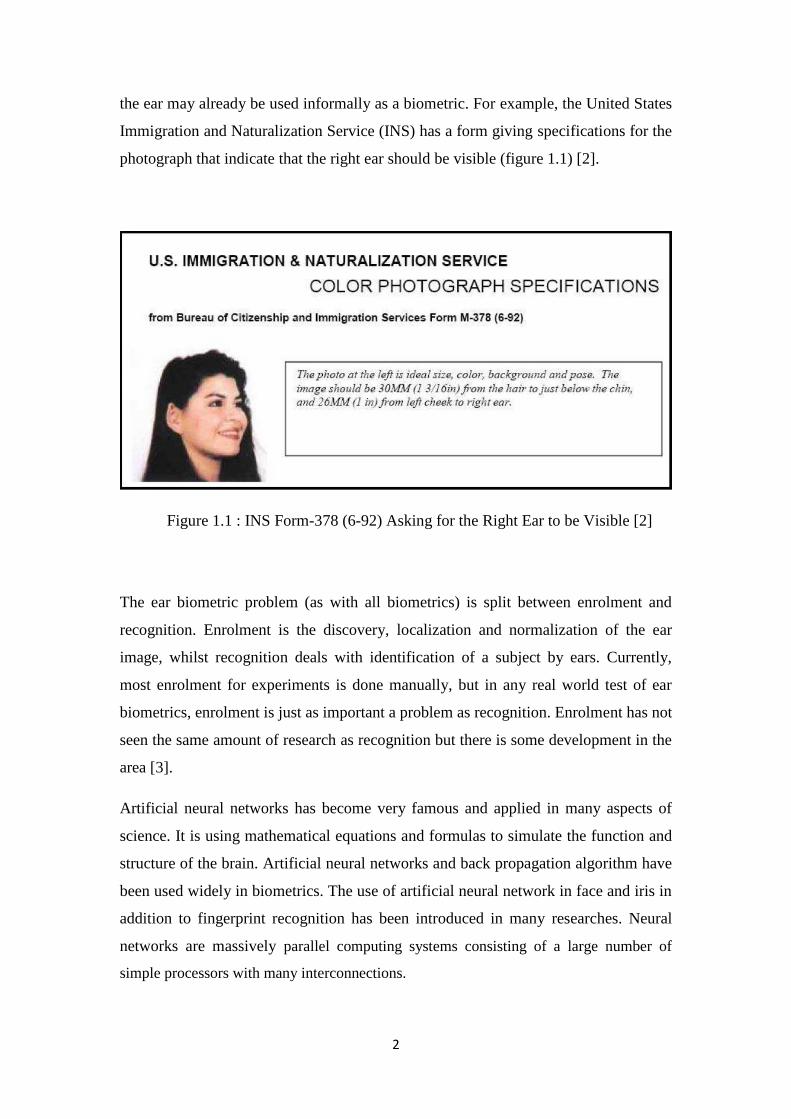
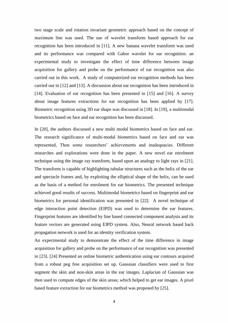
Iris recognition is considered to be one of the exact methods of recognition. The

damage of iris features is less possible compared to the finger or palm print due to the

eyelids. One of the main advantages of iris recognition is its stability during the whole

life, while its small size(figure 2.4) and impossibility of taking its photo from a

distance are the most disadvantages of this method. Also people with blindness or

cataract are difficult to be involved in iris recognition process as it is difficult to

extract information from their iris.

Figure 2.4: Iris [26]

2.5.5 Palm Print

Palm-print is often mentioned with such methods as fingerprints and iris recognition.

Palm-print is also distinctive and can easily be captured with low resolution devices

[24]. The inner surface of palms, has rich features including principal lines, wrinkles,

minutiae points, singular points and texture. These features can be used for uniquely

identifying a person. Currently, there are two types of palm-print research, high

resolution approach and low resolution approach.(figure 2.5) High resolution

approach is suitable for forensic applications while low resolution approach is suitable

for commercial applications [21].

Human beings were interested in the palm lines for fortune telling long time ago. In

this century, scientists discovered that the palm lines were associated with some

genetic diseases including Down syndrome, Aarskog syndrome, Cohen syndrome and

fetal alcohol syndrome [21]. The palm of each person consists of principle lines,

wrinkles secondary lines and ridges. Palm also contains such information as texture,

14

indents and marks which are used during the comparison of one palm with another

[24].

Figure 2.5: High and low resolution palm print images [27].

2.5.6 Signature

It is a behavioral biometric, is widely accepted in governmental, legal and commercial

transactions. Each person can have several signatures for different applications.

Nevertheless, a signature cannot uniquely identify a person. Many factors can

influence the consistency of signatures such as emotional and physical conditions.

Furthermore, professional forgers are capable of reproducing signatures to fool

recognition systems [21].

2.5.7 Voice

Voice for humans is claimed to be unique like walking way and sent. It is how ever

taking long time to analyze the voice and identify a person. To identify the person

with the help of voice print, a sample of speech should be taken. This sample is

analyzed. Different multiple measurements are taken and the results are presented in

the form of the algorithm.

15

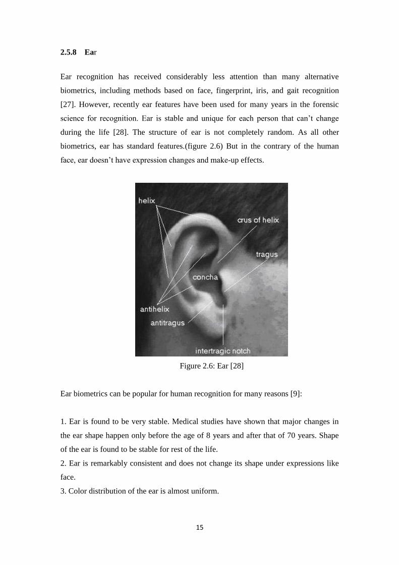
2.5.8 Ear

Ear recognition has received considerably less attention than many alternative

biometrics, including methods based on face, fingerprint, iris, and gait recognition

[27]. However, recently ear features have been used for many years in the forensic

science for recognition. Ear is stable and unique for each person that can‟t change

during the life [28]. The structure of ear is not completely random. As all other

biometrics, ear has standard features.(figure 2.6) But in the contrary of the human

face, ear doesn‟t have expression changes and make-up effects.

Figure 2.6: Ear [28]

Ear biometrics can be popular for human recognition for many reasons [9]:

1. Ear is found to be very stable. Medical studies have shown that major changes in

the ear shape happen only before the age of 8 years and after that of 70 years. Shape

of the ear is found to be stable for rest of the life.

2. Ear is remarkably consistent and does not change its shape under expressions like

face.

3. Color distribution of the ear is almost uniform.

16

4. Handling background in case of ear is easy as it is very much predictable. An ear

always remains fixed at the middle of the profile face.

5. Ear is unaffected by cosmetics and eye glasses.

6. Ear is a good example of passive biometrics and does not need much cooperation

from the subject. Ear data can be captured even without the knowledge of the subject

from a distance.

7. Ear can be used in a standalone fashion for recognition or it can be integrated with

the face for enhanced recognition.

Researchers have suggested that the shape and appearance of the human ear is unique

to each individual and relatively little change occurs during the lifetime of an adult

[2]. The potential for using the ear‟s appearance as a means of personal identification

was recognized and advocated as early as 1890 by the French criminologist Alphonse

Bertillon. Unlike face recognition, ear is also not affected by factors such as mode or

health. The outer shape of ear remain same and is not affected by age [1].

2.5.9 Other Biometrics

Other biometrics includes gaits, lip prints, brain signals, teeth, retinas, odor,

keystrokes, heights, weights and genders have been proposed. They have different

characteristics and different potential applications.

17

CHAPTER THREE

ARTIFICIAL NEURAL NETWORKS

3.1 Overview

The idea of artificial neural network appeared in the 5th decade of the 20th century. It

was firstly a try of imitating the structure and function of the human brain. However,

the philosophical and psychological perspective of such ideas were originated and

studied by great thinkers like Plato and Aristotle. The first paper on neural network

was published in 1943 by McCuloch and Pitts presenting a simple neuron that

produces 0 or 1[30].

This chapter of the thesis will be concerned by the study of the structure and function

of Artificial Neural Network. It will be especially discussing the back-propagation

learning algorithm of ANNs.

After the first paper proposing the neural network as a processing network, many

works has been proposed successively. In 1949, Hebb proposed a learning process

which has become the starting of the neural network learning algorithms. In 1962,

Rosenblatt was able to prove the convergence of a learning algorithm. that means the

iterative adjustment of the weights of the network until obtaining a desired set of

outputs. The use of single layer neural networks was unable to present an efficient

solution for a lot of types of problems. Although it was believed that multilayer

network can offer better performance for such problems, but there was no efficient

learning algorithm which can insure the convergence of the network.

The revolution in the development of ANNs happened in the middle of the 9th

decade

of the 20th

century. When researchers invented an algorithm for training multilayer

ANNs.

3.2 Introduction of ANNs

An artificial neural network is a system composed of many simple processing

elements operating in parallel to compose a functional network. The function of these

elements is determined by the structure of the network, the strength of the connections

between its elements, and the processing manner performed in the nodes. The

structure of ANNs is inspired by the architectural structure biological nervous system.

18

The biological nervous system uses millions of interconnected parallel elements to

obtain high computing efficiency.

An artificial neural network is a huge parallel processor having natural propensity for

storing experiential knowledge and making it available for use [29]. It resembles the

brain in two aspects:

Knowledge is gained by simple learning process.

The information is stored in the synaptic weights which represent the inter-neural

connection strength.

The neuron is like a MISO (multiple inputs single output) system, its output strength

is determined by the strengths of its different inputs. The signals of all neurons are

summed and compared to a threshold defined by the user to determine if the output

shall be excited.

3.3 Biological Neuron

The brain is composed of billions of neurons interconnected between each other with

billions of interconnections. Each biological neuron is composed of five parts: cell

body, nucleus, dendrites, synapse, and axons.(figure 3.1) Dendrites are connected to

the cell body. They are responsible for receiving a signal from the connection point

called synapse. Synaptic junction can both receive and transmit information. The

received signal is transmitted chemically changing the electrical potential inside the

cell body. If the potential exceed a defined threshold, a pulse of defined strength and

threshold is generated through the axon to the other neurons [30]. The neuron is able

to respond to the total of its inputs aggregated within a short time interval called the

period of latent summation. The membrane can be considered as a shell, which

aggregates the magnitude of the incoming signals over some duration. Specifically,

the neuron generates a pulse response and sends it to its axon only if the conditions

necessary for firing are fulfilled [31].

19

Figure 3.1: Basic biological neuron [31].

3.4 Artificial Neuron And Neural Networks

Artificial neural network (ANN) is a discipline that draws its inspiration from the

incredible problem-solving abilities of nature‟s computing engine, the human brain,

and endeavors to translate these abilities into computing machine which can then be

used to tackle difficult problems in science and engineering. However, all Artificial

neural network paradigms involve a learning phase in which the neural network is

trained with a set of examples of a problem [31]. An artificial neuron is designed to

mimic the basic functions of biological neurons [30]. It computes the sum of the

weights applied to its inputs. This sum is the equivalent of the electrical potential

transmitted through the cell body in the biological neuron. The output is then passed

to an activation function to determine if it is enough to activate the neuron or not. The

equation describing the sum in the ANN is: (figure 3.2)

ij iij

NET w x (3.1)

20

Figure 3.2: Sample structor of ANN

3.5 Adaptive Networks And Systems

3.5.1 Activation Function

After the processing of inputs with associated weights and finding the sum of them,

an activation function is used to determine whether the output is to be activated or not.

Some activation functions are used to determine how much the processed input will

share in constructing the total output of the network. There are many types of

activation functions in artificial neural networks:

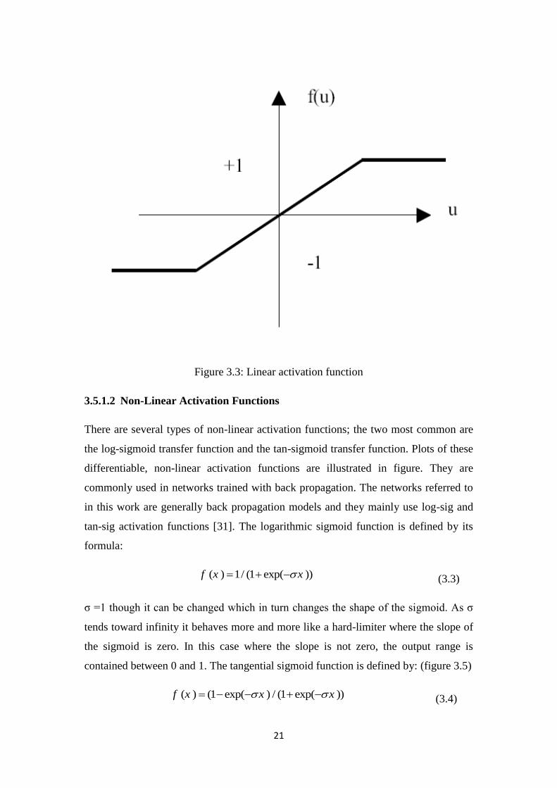
3.5.1.1 Linear Activation Function

This type of activation function is known by its function defined by: (figure 3.3)

1 1

( ) 1 1

1 1

x

f x x x

x

(3.2)

21

Figure 3.3: Linear activation function

3.5.1.2 Non-Linear Activation Functions

There are several types of non-linear activation functions; the two most common are

the log-sigmoid transfer function and the tan-sigmoid transfer function. Plots of these

differentiable, non-linear activation functions are illustrated in figure. They are

commonly used in networks trained with back propagation. The networks referred to

in this work are generally back propagation models and they mainly use log-sig and

tan-sig activation functions [31]. The logarithmic sigmoid function is defined by its

formula:

( ) 1/ (1 exp( ))f x x (3.3)

σ =1 though it can be changed which in turn changes the shape of the sigmoid. As σ

tends toward infinity it behaves more and more like a hard-limiter where the slope of

the sigmoid is zero. In this case where the slope is not zero, the output range is

contained between 0 and 1. The tangential sigmoid function is defined by: (figure 3.5)

( ) (1 exp( ) / (1 exp( ))f x x x (3.4)

22

Where it differs from the logarithmic sigmoid in that its output is limited by the -1 and

one as illustrated in figure.(figure 3.4)

Figure 3.4: Logarithmic sigmoid activation function.

Figure 3.5: Tangential sigmoid activation function

-100 -80 -60 -40 -20 0 20 40 60 80 1000

0.2

0.4

0.6

0.8

1

x

f(x)

-100 -80 -60 -40 -20 0 20 40 60 80 100-1

-0.8

-0.6

-0.4

-0.2

0

0.2

0.4

0.6

0.8

1

x

f(x)

23

3.5.1.3 Hard Limit ( Threshold Function)

A threshold (hard-limiter) activation function is either a binary type(figure 3.6) or a

bipolar type(figure 3.7) as shown in Figures.

Figure 3.6: Binary activation function

Figure 3.7: Bipolar activation function

3.6 Learning Methods of ANN

In general, learning is a relatively permanent change in behavior brought about by

experience. Learning in neural networks is a more direct process, and we typically can

capture each learning step in a distinct cause-effect relationship. The knowledge of a

-3 -2 -1 0 1 2 3

0

0.5

1

1.5

2

x

f(x)

f(x)

-3 -2 -1 0 1 2 3-2

-1.5

-1

-0.5

0

0.5

1

1.5

2

x

f(x)

24

neural network is stored in the synapses, which are the weights of the connections

between the neurons [31]. A neural network has to be configured such that the

application of a set of inputs produces the desired outputs. Various methods to set the

strengths of the connections exist. One way is to set the weights explicitly using a

priori knowledge. Another way is to train the neural network by feeding it teaching

patterns and letting it change its weights according to some learning rule [32].

Dependent on the previous context, the learning methods of ANN can be divided into

two categories: supervised and Un-supervised learning methods.

3.6.1 Unsupervised Learning

In this method, a unit is trained to respond to clusters of pattern within the input. In

this paradigm the system is supposed to discover statistically salient features of the

input population. Unlike the supervised learning paradigm there is no a priori set of

categories into which the patterns are to be classified rather the system must develop

its own representation of the input stimuli [32].

3.6.2 Supervised Learning

In this method of learning, the network is trained a prior by providing it with

examples. These examples are exactly the same as those given to a student in school.

the network is given inputs examples with associated outputs. After each train of the

network, a measure of the learning error is applied and the weights of the network are

adjusted based on that measure. The training is stopped whenever the error between

the target and actual output of network is acceptable or a maximum number of trains

is reached. One of the most important supervised learning methods which will be our

subject of study is the back-propagation algorithm. Back propagation algorithm will

be explained and discussed in details in the next few pages. It will be used then for the

rest of our work as it has proved its efficiency as a learning method for ANN

applications.

3.7 Back Propagation Learning Algorithm of ANNs

A back propagation neural network uses a feed-forward topology, supervised

learning, and back propagation learning algorithm. This algorithm was responsible in

large part for the re-emergence of neural networks in the mid 1980s. Back

propagation is a general purpose learning algorithm.(figure 3.8) It is powerful but also

25

expensive in terms of computational requirements for training. A back propagation

network with a single hidden layer of processing elements can model any continuous

function to any degree of accuracy (given enough processing elements in the hidden

layer) [33].

Figure 3.8: Back propagation network

Although many improvements on basic back propagation algorithm have been

proposed and applied, still the basic algorithm is the most widely used and famous

one. That is mainly due to the fact that it is simple and easy to be understood; in

addition to that it works for a wide range of problems [33]. Back propagation can be

divided into three steps:

The input data is presented to the input layer of the ANN, the input non processing

layer passes this data to the hidden layer where the data is processed with weights and

using summing and activation functions. The output of the hidden layers is then

passed to the output layers. The input data of output layer is processed as in hidden

layers. The last output is then compared to the desired targets and error is generated.

26

The generated error is then back propagated through the output and hidden layers; that

is the weights of the output and hidden layers are readjusted using formulas of the

error which guarantee the convergence of the error toward null value.

After the adjustment of the weights, the inputs are passed again to the input, hidden,

and output layers and a new error is calculated in a second iteration and vice versa.

The three mentioned step continue being applied until the error of the training

becomes less than an acceptable set value or a maximum number of iterations is

achieved. The flowchart shown in figure (3.9) explains the Back Propagation

algorithm.

Two major learning parameters are used to control the training process of a back

propagation network. The learn rate is used to specify whether the neural network is

going to make major adjustments after each learning trial or if it is only going to make

minor adjustments. Momentum is used to control possible oscillations in the weights,

which could be caused by alternately signed error signals. While most commercial

back propagation tools provide anywhere from 1 to 10 or more parameters for you to

set, these two will usually produce the most impact on the neural network training

time and performance [33].

27

Start

Reading Images and ANN

Parameters

Preprocessing of the images in MATLAB

Set random hidden and output weights and biases

Construct the input Outputmatrix of

ANN

Training of the network using Back Propagation

Algorithm, calculation of outputs for each pattern

Calculating the MSE

Preprocessing of the images in MATLAB

If MSE<Epsilon

Or

Number of Iterations > max. iterations

Yes

No

Save the last Parameters and weights

Display results and Error

End

Figure 3.9: Block diagram of the training process (flowchart)

28

The back propagation is a method based on error minimization theory and by

searching the least squared error using the gradient descent. Since this method

requires computation of the gradient of the error function at each iteration step, we

must guarantee the continuity and differentiability of the error function at all time.

That implies the use of differentiable continuous function as an activation function.

This condition can be guaranteed by the use of the sigmoid tangent or logarithm

mentioned previously. The logarithmic sigmoid defined by the function (3.5) is

differentiable and its derivative is given by (3.6).

1( )

1 xf x

e

(3.5)

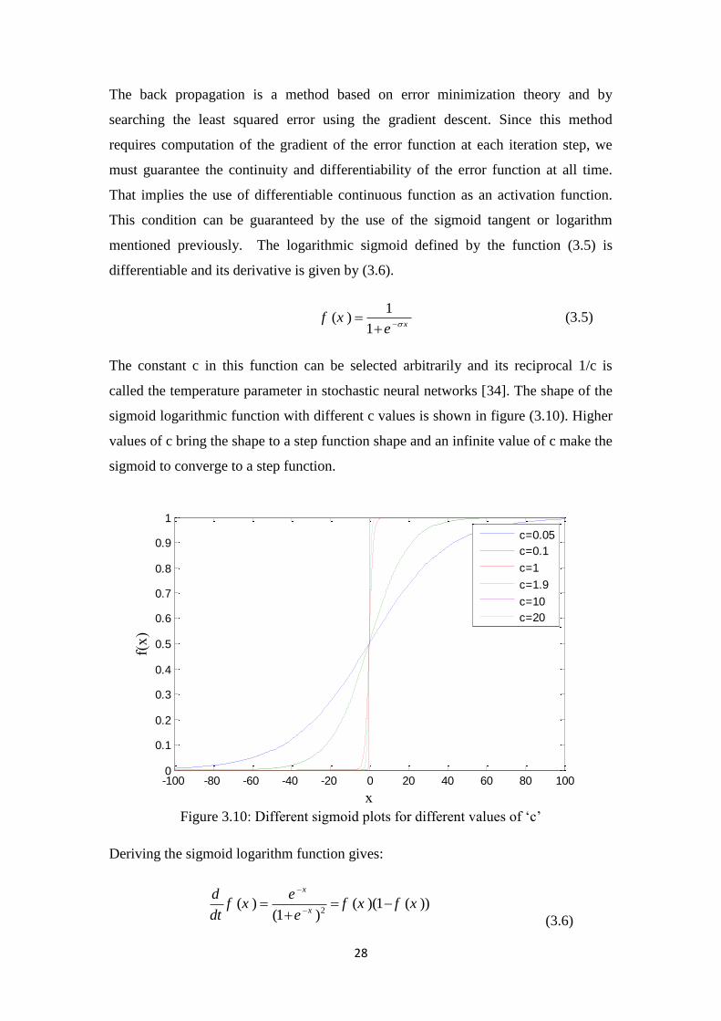
The constant c in this function can be selected arbitrarily and its reciprocal 1/c is

called the temperature parameter in stochastic neural networks [34]. The shape of the

sigmoid logarithmic function with different c values is shown in figure (3.10). Higher

values of c bring the shape to a step function shape and an infinite value of c make the

sigmoid to converge to a step function.

Figure 3.10: Different sigmoid plots for different values of „c‟

Deriving the sigmoid logarithm function gives:

2

( ) ( )(1 ( ))(1 )

x

x

d ef x f x f x

dt e

(3.6)

-100 -80 -60 -40 -20 0 20 40 60 80 1000

0.1

0.2

0.3

0.4

0.5

0.6

0.7

0.8

0.9

1

x

f(x)

c=0.05

c=0.1

c=1

c=1.9

c=10

c=20

29

3.7.1 Learning Problem

The neural network represents a chain of function compositions which transform an

input to an output vector (called a pattern). The network is a particular

implementation of a composite function from input to output space, which we call the

network function. The learning problem consists of finding the optimal combination

of weights so that the network function approximates a given function “f” as closely

as possible. However, we are not given the function “f” explicitly but only implicitly

through some examples [34].

Considering a neural network with n inputs and m outputs. It can also consist of any

arbitrary number of hidden units. The weights of the network are real numbers

selected randomly. Given a set of inputs and outputs {(x1, t1 ),(x2, t2 ), . . . , (xp, tp )}

consisting of p ordered pairs of n and m vectors representing the input and output

patterns. When the input xi from the training set is presented to the network, it

produces an output oi generally different from the target ti. Our goal is to have

identical outputs oi and targets ti for all inputs and outputs of the set. In other words,

the aim is to minimize the error function of the network defined by:

2

1

1( )

2

p

i iit o

(3.7)

After minimizing this function for the training set, new unknown input patterns are

presented to the network and we expect it to interpolate. The network must recognize

whether a new input vector is similar to learned patterns and produce a similar output

[34].

The back-propagation algorithm is used to find a local minimum of the error function.

The network is initialized with randomly chosen weights. The gradient of the error

function is computed and used to correct the initial weights. Our task is to compute

this gradient recursively. The network is said to be learned if the error arrives a

minimum acceptable value and all or most of patterns are recognized correctly.

After the end of learning process of network, arbitrary patterns can be presented to the

network in a test process. The results of the network are then threshold using a

threshold chosen based on the application. High threshold values can be used in

30

health, military, or security applications, while smaller thresholds can be accepted for

less important applications.

This chapter has discussed the structure and function of neural networks. The

development of the ANN has be presented through the 20th

century has been

presented. A study of back-propagation algorithm has been presented and discussed.

The application of back propagation learning algorithm for the ear recognition will be

discussed and studied in the next chapter. Samples from 54 persons left and right ear

were taken and presented to the neural network for learning process. Results and

discussions about the used methods and procedures will be detailed.

31

CHAPTER FOUR

EAR RECOGNITION EXPERIMENTAL RESULTS

4.1 Overview

An ear recognition system must deal with two basic problems; the extraction of the

most important features of the ear, and the recognition of these ears or for whom they

belong.

This chapter presents a detailed discussion about the back-propagation based ear

recognition system. The use of the back propagation in the recognition of different

right and left ear images is discussed and presented. 54 different pairs of ears are used

in the identification of 54 persons who are the sample of this thesis. The ears taken

from these sample persons are then treated with different types of noises to provide

different example for the neural network. The sets of real and noisy images are

preprocessed and then presented to the ANN using the back propagation learning

process in the training phase. After that a simple test is applied to check the ability of

network to recognize processed ear photos.

The chapter presents the methodology of the research and the different steps of it;

starting by collecting the data base and ending with the testing phase. The application

of the noise and processing of the images is an important phase in the recognition

procedure. It is discussed in this chapter with presentation of different processed

features and their effect.

The processing of the images data using MATLAB including adding the noise to the

pictures in addition to resizing and changing the type of images to reduce processing

cost. The pre-processing phase is a very important phase for a successful recognition

system. The choice of image sizes in addition to the methodology of working affect

directly the results of the program in addition to the time of working.

4.2 Database Collection

The first step in this work was the data base collection. All the images where collected

from the students of the computer engineering department in Near East University.

32

The photos of ears of 54 students were taken using a 13 megapixel Samsung camera.

Photos included the right and the left ears images for each person. A distance of 10

centimeters was arbitrary chosen between the camera‟s lens and the ear. An angle of

90 degrees was used to take the photos.(figure 4.1) The photos were then arranged

and processed using Photoshop program. The photos were prepared such that just the

features of the ears appear in the picture. Any empty spaces or other features like hair

where manually removed from the pictures. The preprocessing phase includes the

changing the images to gray scale images, resizing images, normalization of images

data, and adding noise to images.(figure 4.2)

Figure 4.1: Ear photo collection data

33

Read the RGB image

Convert RGB image to gray

scale image

Reduce the size of image

to 50*50

Add different types of Noise

to the images

Normalizing the pixels

values of the image

Convert the image matrix to

vector of size 50*50

Building the input training and

test matrix containing all images

vecors

Send the input matrix to the network

training and test processing

Figure 4.2 : Block diagram of the preprocessing phase of the training and test images.

4.3 General Experiment

Many experiments were carried out on the set of image until arriving suitable

parameters of the neural network in the training process. In the training process of the

neural network 8 sets of normal and noisy images were used. The first set represented

the normal images of the ear. The other sets were noised using MATLAB program.

Different types of noises were used in the training like Gaussian and salt and pepper

34

noise. The MATLAB code used for adding different types of noise in addition to the

noise rates are presented in Appendix A,

The Noises added here in the training process were:

- Gaussian white noise of mean 0.02 and variance 0.0018 and 0.005 to the

normalized image.

- Speckle with multiplicative noise using the equation J = I + n*I, where n is

uniformly distributed random noise with mean 0 and variance 0.04 and 0.08.

- Salt and pepper noise with density 0.05 and 0.01.

A sample of the original and noisy images is shown in figure 4.3 and figure 4.4:

Figure 4.3: Sample of the images used in the training (first person left).

Figure 4.4: Sample of the images of training (first person right).

35

The images of the figure 4.3 and 4.4 represent the training sample of the first person.

These images were preprocessed before being fed to the network. The preprocessing

of the images passes by different phases. The first phase after reading the image in

RGB scale is to change it into gray scale image. The gray scale image represents each

pixel of the image by an unsigned eight bit integer (0-255). This number is the

concentration of white color in the pixel. The pixel is black if its value is zero,

increasing the value increase the white concentration until it maximum in the white

color with the value of 255. In the rgb scale images each pixel is presented using 3

different values; each one of these three values presents the concentration of the three

base colours, red, green, and blue. Using the gray scale image reduces the image size

by two thirds of its original rgb scale size. That operation reduces the calculation

efforts carried by the program with aboutly no effect on the accuracy of the program.

After the process of changing image scale, the size of the image has to be reduced to

an acceptable size to make easier the operations on smaller images in addition to

reduce the processing cost of the program. The size of images was chosen to be

50*50. Figure 4.5 shows the original rgb image and gray scale image in addition to

the resized image.

Figure 4.5: Original RGB image(size(3100*2100)) and Gray scale

image(size(3100*2100)).

RGB image GRAY scale image

36

Figure 4.6: Resized gray scale image (size(50*50)).

The resized image is after that normalized in order to limit the inputs of the ANN by 0

and 1. This operation reduces the processing costs and learning time. The processed

images must be arranged and fed to the neural network such that the one ear

information is processed in each iteration. In the next iteration, an image of a different

ear should be presented to the network until the last image. After finishing all images,

the operation must be repeated from the beginning until the network learns. In order

to make easier the mentioned operation, a small routine was written using MATLAB

to arrange each picture‟s pixels in a vector. The vectors are then arranged in a big

matrix which will be fed column by column to the network. The desired output of the

network was chosen arbitrary and also arranged in an output matrix which was

presented to the network.

4.4 Training of the network

As mentioned in the previous chapters, back-propagation learning algorithm was used

in the training process of the network. After feeding the pictures to the network, three

different experiments were carried out with different network parameters in order to

evaluate the performance of our procedure. In each experiment different parameters of

the network were used. The test was performed with different pictures (noise level)

for each experiment.

37

Experiment 1:

The back-propagation process was started with the next parameters:

Table 4.1: Parameters of the network in first experiment.

Number of input neurons 2500

Experimental number of hidden neurons 200, 240

Number of output neurons 54

Experimental initial learning rate 0.09

Experimental momentum factor 0.3

Minimum error 0.0005 achieved

Number of iterations 4037

Maximum iterations 20000

Training time 20 min 55 sec

Testing time 0.110756 sec

Figure 4.7 shows the mean squared error curve obtained in the training process. In the

hidden layers two activation functions were used, the first is logsig activation

function, while the second was tansig function; a logsig function was also used in the

output layer.

Figure 4.7: Curve of MSE in the training.

0 500 1000 1500 2000 2500 3000 3500 4000

10-3

10-2

10-1

Epocs

MS

E

MSE Curve

38

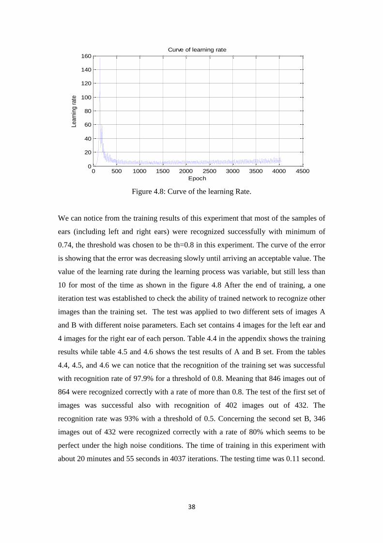
Figure 4.8: Curve of the learning Rate.

We can notice from the training results of this experiment that most of the samples of

ears (including left and right ears) were recognized successfully with minimum of

0.74, the threshold was chosen to be th=0.8 in this experiment. The curve of the error

is showing that the error was decreasing slowly until arriving an acceptable value. The

value of the learning rate during the learning process was variable, but still less than

10 for most of the time as shown in the figure 4.8 After the end of training, a one

iteration test was established to check the ability of trained network to recognize other

images than the training set. The test was applied to two different sets of images A

and B with different noise parameters. Each set contains 4 images for the left ear and

4 images for the right ear of each person. Table 4.4 in the appendix shows the training

results while table 4.5 and 4.6 shows the test results of A and B set. From the tables

4.4, 4.5, and 4.6 we can notice that the recognition of the training set was successful

with recognition rate of 97.9% for a threshold of 0.8. Meaning that 846 images out of

864 were recognized correctly with a rate of more than 0.8. The test of the first set of

images was successful also with recognition of 402 images out of 432. The

recognition rate was 93% with a threshold of 0.5. Concerning the second set B, 346

images out of 432 were recognized correctly with a rate of 80% which seems to be

perfect under the high noise conditions. The time of training in this experiment with

about 20 minutes and 55 seconds in 4037 iterations. The testing time was 0.11 second.

0 500 1000 1500 2000 2500 3000 3500 4000 45000

20

40

60

80

100

120

140

160

Epoch

Learn

ing r

ate

Curve of learning rate

39

Experiment 2:

In this experiment, the parameters of the network have been changed and new training

and test processes have been applied. Results of test and training were presented and

tabulated. The training parameters are given in the next table:

Table 4.2: Parameters of the network in second experiment.

Number of input neurons 2500

Experimental number of hidden neurons 100, 150

Number of output neurons 54

Experimental initial learning rate 0.09

Experimental momentum factor 0.2

Minimum error 0.00005

Number of iterations 17244

Maximum iterations 20000

Training time 103min 10sec

Testing time 0.085397

The curve of the error is shown in figure 4.9, where we can notice that it was

decreasing with good rate and reached a good value. A minimum error of 0.00005

was reached after 103 minutes and 10 seconds with total of 17244 iterations. Also the

achieved MSE was better.

Figure 4.9: MSE curve in experiment 2.

100

101

102

103

104

105

0

0.05

0.1

0.15

0.2

0.25

Epocs

MS

E

40

Table 4.7 in the appendix shows that all the training images were recognized

successfully in this experiment with a rate of 100% under a threshold of 0,8. The

training results show that the network was perfectly trained with high efficiency. For

the test purpose, the sets of images A and B were passed through the network and the

results were checked. Table 4.8 shows that 97.6% of the images of set A were

recognized with threshold of 0.5, 422 images out of 432 were perfectly recognized.

While for the set B results we can notice that just 373 images out of 432 images were

recognized using the same network due to the high noise effects added. The

recognition rate was 86.3% which is considered excellent. The results are shown in

Table 4.9. The difference in efficiency between the recognition results of sets A and B

is due mainly to the amounts of noise added to both sets. The images of set B were

noisier and less clear than the set A. a recognition rate of 86.3% can be considered

high under such conditions of noise.

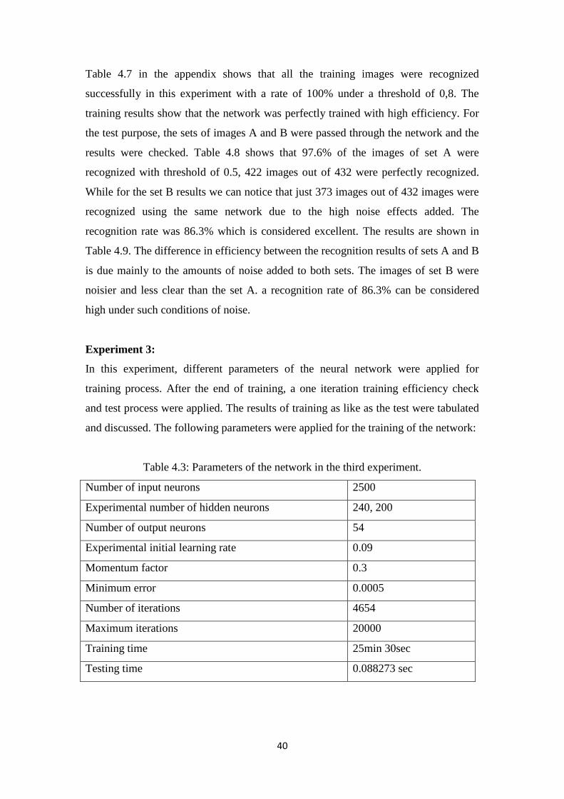
Experiment 3:

In this experiment, different parameters of the neural network were applied for

training process. After the end of training, a one iteration training efficiency check

and test process were applied. The results of training as like as the test were tabulated

and discussed. The following parameters were applied for the training of the network:

Table 4.3: Parameters of the network in the third experiment.

Number of input neurons 2500

Experimental number of hidden neurons 240, 200

Number of output neurons 54

Experimental initial learning rate 0.09

Momentum factor 0.3

Minimum error 0.0005

Number of iterations 4654

Maximum iterations 20000

Training time 25min 30sec

Testing time 0.088273 sec

41

As shown in the table, the network has achieved an error of 0.0005 in 25 minutes and

30 seconds with 4654 iteration. The training time has been reduced to 25 minutes and 30

seconds. The time of one iteration test was 0.0882 second. The results of this experiment have

shown good recognition rate and high performance. As shown in tables 4.10, 4.11, and

4.12 we can notice that the training recognition was 99.3% with 658 recognized

images out of 864. The threshold was chosen to be 0.8 while in the test a value of 0.5

was used. The set A test gave a recognition rate of 94.4% with 408/432 images

recognized successfully. In the set B, 358 images out of 432 were recognized with a

rate of 82.8%. We can notice also that the recognition of set A was better than Set B.

The results obtained from the different experiments prove the efficiency of the

artificial neural networks in human identification using ear patterns. The next table

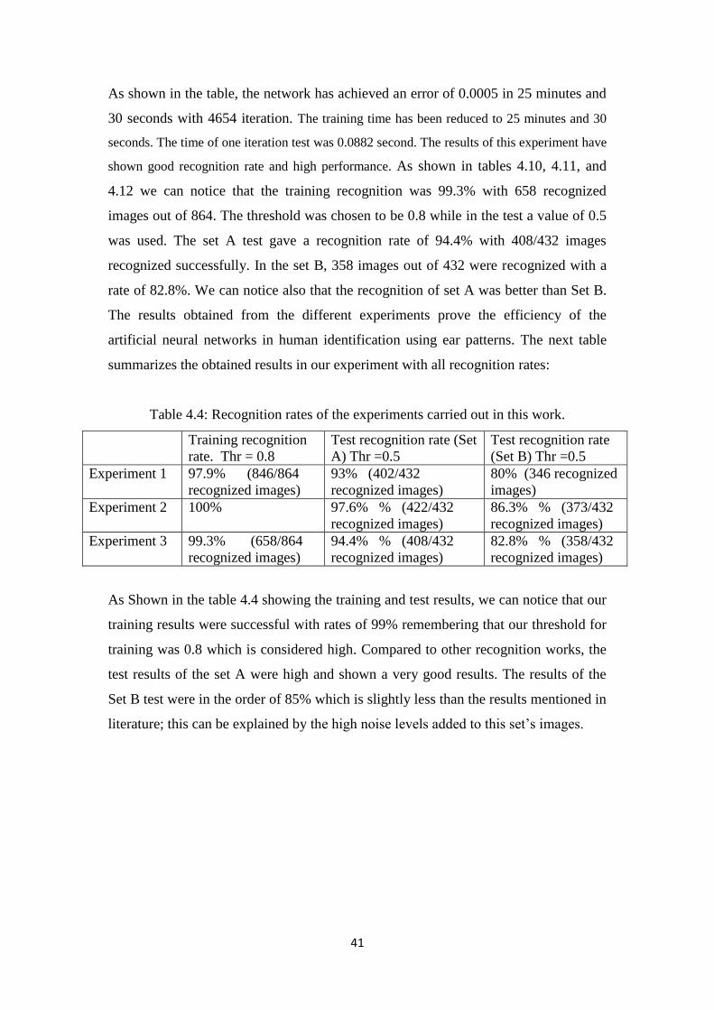
summarizes the obtained results in our experiment with all recognition rates:

Table 4.4: Recognition rates of the experiments carried out in this work.

Training recognition

rate. Thr = 0.8

Test recognition rate (Set

A) Thr =0.5

Test recognition rate

(Set B) Thr =0.5

Experiment 1 97.9% (846/864

recognized images)

93% (402/432

recognized images)

80% (346 recognized

images)

Experiment 2 100% 97.6% % (422/432

recognized images)

86.3% % (373/432

recognized images)

Experiment 3 99.3% (658/864

recognized images)

94.4% % (408/432

recognized images)

82.8% % (358/432

recognized images)

As Shown in the table 4.4 showing the training and test results, we can notice that our

training results were successful with rates of 99% remembering that our threshold for

training was 0.8 which is considered high. Compared to other recognition works, the

test results of the set A were high and shown a very good results. The results of the

Set B test were in the order of 85% which is slightly less than the results mentioned in

literature; this can be explained by the high noise levels added to this set‟s images.

42

CONCLUSIONS

There is an increasing need for more secure and easy identification methods. The use

of passwords and security codes is becoming more and more difficult with the

development of information technology. Over more, the explosion in the internet

services, banks services, credit cards, debit cards involve the need for remembering a

huge number of pass phrases which – in addition to be very hard task – can be lost

easily and cost a lot to reinitialize. The need also for more secure systems in airports

and police services in order to fight the crime has increased. All these factors have

pushed the researchers toward finding more natural, easy, and highly secure

identification methods. One of the most important methods of identification which

became widely used is the biometrics. Although the use of ear as unique and stable

feature of the human being has been introduced into biometrics since many years, it is

still need for more attention of the researchers due to its simplicity and good

performance.

This work has been carried out in the goal of giving more attention for the use of ear

as an identification method. Combining the use of ear as a biometric feature with the

use of artificial neural network can be considered as a promising idea for the near

future as the neural networks is showing very fast development in the last years.

Artificial neural networks have proved its ability for solving many non-linear

problems efficiently with a minimum effort.

From the experiments carried out in this thesis and the results obtained we conclude

that the use of the neural network for ear recognition and persons Identification was

successful. The application of different noise on the ear‟s images has led to reduction

of recognition rate. Many experiments were carried out with different network

parameters and noise levels. The first experiment has given a training recognition rate

of 97.9%. The test recognition rate of 93% for the set A was achieved. Increasing the

level of noise has affected slightly the recognition capability of the neural network;

that is, in set B the recognition rate has been reduced to 80%. The training time in the

first experiment was about 20 minutes and can be considered fast. In a second

experiment the parameters of the network has been changed. The maximum error has

been changed to 0.1 of that used in experiment one. The recognition rate of 100% in

the training and 97.6% for the test of set A was achieved. The recognition rate of set

43

B was 86.3%. The reduction of maximum error has increased the accuracy of the

network recognition, but the time of training increased to more than100 minutes. This

is relatively long time if compared to the training time of first experiment. The third

experiment has given a recognition rate of 99.3% in the training, with 94.4% and

82.8% recognition rate in the test of set A and B respectively.

Using the network for the identification of both right and left ear images at once has

shown a good level of success with high performance. After finishing the work we

can conclude that the use of ANN in the ear recognition for person identification can

be achieved with high accuracy and can give good levels of security. The neural

networks can be considered as a very good method for recognition and biometrics

identification.

The results obtained in this work proved that the use of ANN for persons‟

identification using ear recognition is a promising idea. The results obtained were

very successful in term of identification rate and time efficiency. The work carried out

in this thesis directs toward making more effort in the subject and paying more

attention for the ANN based ear recognition process. It opens the doors for more

intense and large work in the science of biometrics. As a future work, this thesis

proposes the use of multi-modal identification based on artificial neural network and a

comparative work between the ANN based ear recognition and the other methods

such as wavelet transform based ear recognition.

44

REFERENCES

[1] Mohamed Ibrahim Saleh, “ Usıng Ears For Human Identıfıcatıon”, Master Thesis,

Blacksburg, Virginia May 2007.

[2] Ping Yan, B.S., M.S. “ Ear Biometrics in Human Identification ”, Graduate

Program in Department of Computer Science and Engineering Notre Dame, İndiana

June 2006.

[3] Alastair H. Cummings, Mark S. Nixon, John N. Carter “Novel Ray Analogy for

Enrolment of Ear Biometrics”, 2010.

[4] Vankadara Nvd Manohar Gaurav Uday Chaudharı Bıswajıt Mohanty,

“Functıon Approxımatıon Usıng Back Propagatıon Algorıthm In Artıfıcıal Neural

Networks”, A Thesıs Submıtted In Partıal Fulfıllment of The Requırements For

The Degree of Bachelor of Technology In Electrical Engineering 2007.

[5] Hazem M. El-Bakry Faculty of Computer Science & Information Systems,

Mansoura University, Egypt&Nikos Mastorakis Technical University of Sofia,

BULGARIA “Ear Recognition by using Neural Networks”, ISSN: 1790-2769.

[6] Hui Chen, Bir Bhanu “Human Ear Recognition in 3D”, IEEE Transactıons On

Pattern analysis, Vol.29, No.4, April 2007.

[7] Md. Mahbubur Rahman, Md. Rashedul Islam, Nazmul Islam Bhuiyan, Bulbul

Ahmed, Md. Aminul Islam. “Person Identification Using Ear Biometrics”, Computer

Science and Engineering Discipline, Khulna University, Khulna-9208, Bangladesh

August 2007.

[8] Sukhdeep Singh, Dr. Sunil Kumar Singla(Assit.Prof.) Electrical & Instrumentation

Engg Dept. Thapar University ,Patiala, India. “ Review on Biometrics and Ear

Recognition Techniques”, International journal of advanced research in computer

science and software engineering. Volüme 3, ıssume 6, june 2013.

[9] Surya Prakash, “Human Recognition using 2D and 3D Ear Images”, PhD Thesis

Indıan Instıtute of Technology Kanpur, Indıa February 2013.

[10] Dasari Naga Shailaja, “A Simple Geometric Approach For Ear Recognition”,

Master Thesis, İndian Instıtute of Technology, Kanpur June 2006.

[11] Mina Ibrahim Samaan Ibrahim, “Wavelet Based Approaches For Detection and

Recognition İn Ear Biometrics”, PhD Thesis, Unıversıty of Southampton June 2012.

45

[12] Mark Burge, Wilhelm Burger, “Ear Biometrics in Computer Vision ” IEEE,2000.

[13] Amioy Kumar, Madasu Hanmandlu, Mohit Kuldeep, And H.M. Gupta,

“Automatic Ear Detection For Online Biometric Applications ”, IEEE 2011.

[14] Ruma Purkait “Ear Biometric: An Aid To Personal Identification”,

Anthropologist Special Volume No. 3: 215-218 (2007).

[15] Barnabas Victor, Kevin Bowyer, And Sudeep Sarkar, “An Evaluatıon Of Face

And Ear Bıometrıcs ”, IEEE 2000.

[16] Ping Yan, Kevinw. Bowyer, “Empirical Evaluation of Advanced Ear Biometrics

”, Proceedings of the Computer Society Conference On Computer Vision And

Pattern Recognition IEEE 2005.

[17] Michał Chora´S, “Image Feature Extraction Methods For Ear Biometrics - A

Survey ”, 6th International Conference On Computer Information Systems And

Industrial Management Applications (CISIM'07) IEEE 2007.

[18] Ping Yan And Kevin W. Bowyer, Fellow, Ieee, “Biometric Recognition Using

3D Ear Shape ”, IEEE Transactıons On Pattern Analysıs And Machıne Intellıgence,

Vol. 29, No. 8, August 2007.

[19] Haijun Zhang, Zengxi Huang And Yibo Li, “An Overview of Multi-Modal

Biometrics Based On Face And Ear ”, Proceedings of The Ieee International

Conference On Automation And Logistics Shenyang, China August 2009.

[20] Daishi Watabe, Hideyasu Sai, Katsuhiro Sakai And Osamu Nakamura, “Ear

Bıometrıcs Usıng Jet Space Sımılarıty ”, Saitama Institute Of Technology, Kogakuin

University, IEEE 2008.

[21] Adams Wai Kin KONG, “Palmprint Identification Based on Generalization of

IrisCode”, A thesis presented to the University of Waterloo in fulfillment of the thesis

requirement for the degree of Doctor of Philosophy in Electrical and Computer

Engineering Waterloo, Ontario, Canada, 2007.

[22] Doctoral thesis Paweł Kasprowski, ” Human identification using eye

movements”, Silesian University of Technology Faculty of Automatic Control,

Electronics and Computer Science Institute of Computer Science, Gliwice 2004.

[23] V.Bhawanı Radhıka, ” Bıometrıc Identıfıcatıon Systems: Feature Level

Clusterıng of Large Bıometrıc Data And Dwt Based Hash Coded Ear Bıometrıc

46

System”, Thesis Submitted n Partial Fulfillment of The Requirements For The Award

of the Degree. Bachelor of Technology (Computer Science And Engg.), May 2009.

[24] Aleksandra Babich,” Biometric Authentication. Types of Biometric

İdentifiers”,Bachelor‟s Thesis Degree Programme in Business Information

Technology 2012.

[25] Cassandra M. Carrillo, Thesis” Contınuous Bıometrıc Authentıcatıon For

Authorızed Aırcraft Personnel: A Proposed Desıgn”, Naval Postgraduate School

Monterey, California June 2003.

[26] Http://Www.Ahmetkakici.Com/Genel/Biyometrik-Tanima-Sistemleri/

[27] Mohamed Ibrahim Saleh,” Usıng Ears For Human Identıfıcatıon”, Thesis

Submitted To The Faculty of Virginia Polytechnic Institute And State University In

Partial Fulfillment of The Requirements For The Degree of Master of Science In

Computer Engineering A. Lynn Abbott, Chairman Chris L. Wyatt Patrick Schaumont

Blacksburg, Virginia, May 2007.

[28] Dasari Naga Shailaja,”A Simple Geometric Approach For Ear Recognition”,A

Thesis Submitted İn Partial Fulfillment of The Requirements For The Degree of

Master of Technology, June 2006.

[29] Bilal F. Alnamiawri, “Sign Language And Gesture Recognition Systemusing

Neural Networks”, A Thesis Submitted To The Graduade School of Applied Sciences

Of NEU 2012.

[30]Nancy Y. Xiao,”Using The Modified Back Probagation Algorithm to Perform Automated

Downlink Analysis”, Master of Engineering Electrical& Computer Science June 1996.

[31] Kiran Kumar Kaki,” Parallelized Backpropagation Neural Network Algorithm

using Distributed System”, Thesis submitted in partial fulfillment of the requirements

for the award of degree of Master of Engineering in Computer Science and

Engineering, January 2009.

[32] Ben Krose Patrick Van Der Smagt,Book ”An Introduction To Neural Network”,

The University of Amsterdam 1996.

[33] Charu Gupta, “Implementatıon of Back Propagatıon Algorıthm (of Neural

Networks) In VHDL”, Thesis Report Submitted Towards The Partial Fulfillment of

Requirements For The Award of The Degree of Master of Engineering (Electronics &

Communication), June 2006.

[34] Chin-Chuan Han, Hsu-Liang Cheng, Chih-Lung Lin, Kuo-Chin Fan,” Personal

Authentication Using Palm-Print Features ”,Pattern Recognition 36 (2003) 371 – 381.

47

APPENDICES

Appendix A

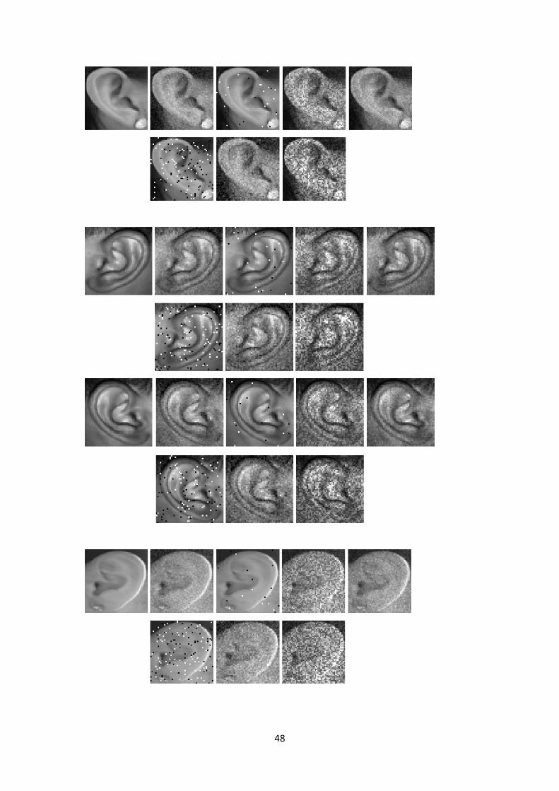
Sample Images of Training Data base

48

49

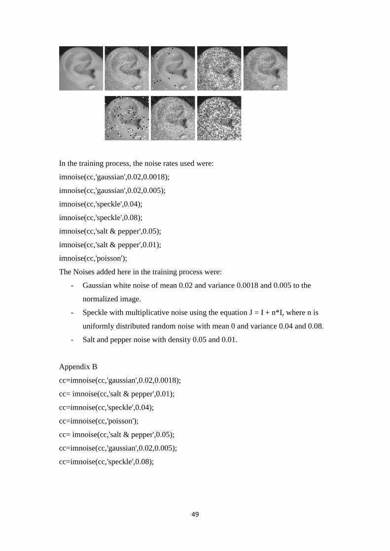
In the training process, the noise rates used were:

imnoise(cc,'gaussian',0.02,0.0018);

imnoise(cc,'gaussian',0.02,0.005);

imnoise(cc,'speckle',0.04);

imnoise(cc,'speckle',0.08);

imnoise(cc,'salt & pepper',0.05);

imnoise(cc,'salt & pepper',0.01);

imnoise(cc,'poisson');

The Noises added here in the training process were:

- Gaussian white noise of mean 0.02 and variance 0.0018 and 0.005 to the

normalized image.

- Speckle with multiplicative noise using the equation J = I + n*I, where n is

uniformly distributed random noise with mean 0 and variance 0.04 and 0.08.

- Salt and pepper noise with density 0.05 and 0.01.

Appendix B

cc=imnoise(cc,'gaussian',0.02,0.0018);

cc= imnoise(cc,'salt & pepper',0.01);

cc=imnoise(cc,'speckle',0.04);

cc=imnoise(cc,'poisson');

cc= imnoise(cc,'salt & pepper',0.05);

cc=imnoise(cc,'gaussian',0.02,0.005);

cc=imnoise(cc,'speckle',0.08);

50

Noise A

switch k,

case 1,

cc=imnoise(cc,'gaussian',0.03,0.0028);

case 2,

cc= imnoise(cc,'salt & pepper',0.15);

case 3,

cc=imnoise(cc,'speckle',0.12);

case 4,

cc=imnoise(cc,'poisson');

end

- Gaussian white noise of mean 0.03 and variance 0.0028 and 0.005 to the

normalized image.

- Speckle with multiplicative noise using the equation J = I + n*I, where n is

uniformly distributed random noise with mean 0 and variance 0.12.

- Salt and pepper noise with density 0.15.

Noise B

switch k,

case 1,

cc=imnoise(cc,'gaussian',0.03,0.02);

case 2,

cc= imnoise(cc,'salt & pepper',0.25);

case 3,

cc=imnoise(cc,'speckle',0.22);

case 4,

cc=imnoise(cc,'poisson');

end

- Gaussian white noise of mean 0.03 and variance 0.02 to the normalized image.

- Speckle with multiplicative noise using the equation J = I + n*I, where n is

uniformly distributed random noise with mean 0 and variance 0.22.

- Salt and pepper noise with density 0.25.

It is clear that the noise levels of set B are very high compared to those of set A.

51

Appendex C

Table 4.5: Training results.

(%) E1R E2R E3R E4R E5R E6R E7R E8R E1L E2L E3L E4L E5L E6L E7L E8L

P1 94 88 93 92 88 94 90 92 93 92 93 92 93 90 95 92

P2 90 89 91 90 92 93 87 87 91 90 88 92 91 91 91 95

P3 92 94 93 84 90 82 92 85 89 86 90 83 92 89 95 94

P4 93 92 91 89 93 90 92 96 91 92 91 91 91 85 90 92

P5 84 87 84 85 81 93 86 93 89 90 90 88 88 88 91 97

P6 86 79 85 89 87 77 80 80 90 91 92 84 93 85 85 85

P7 93 95 93 93 92 94 92 92 87 86 87 91 87 88 88 92

P8 83 92 87 84 86 81 82 83 86 87 79 83 84 82 91 81

P9 90 91 90 91 87 88 87 86 83 93 84 87 88 82 92 85

P10 91 91 89 89 87 87 95 92 90 94 93 89 86 79 92 93

P11 91 90 92 91 90 94 82 84 92 91 90 94 91 86 92 91

P12 89 92 86 81 88 80 96 93 87 89 86 90 85 78 92 86

P13 82 82 79 78 74 87 89 81 81 74 78 92 84 87 75 87

P14 93 94 92 92 93 92 92 89 86 89 87 93 91 83 91 90

P15 87 85 89 90 89 83 91 93 83 86 86 87 78 85 94 85

P16 92 84 93 84 86 95 94 95 93 80 91 82 94 89 95 80

P17 88 92 90 85 90 89 92 94 94 93 92 86 92 90 91 85

P18 86 86 88 87 90 92 89 91 89 91 85 90 87 86 88 93

P19 89 84 87 90 88 81 85 79 90 89 89 79 92 90 90 95

P20 93 95 94 90 93 95 96 93 89 92 90 92 89 89 92 89

P21 93 95 93 93 92 94 93 92 94 93 94 93 93 84 96 92

P22 93 91 93 93 89 96 87 82 91 92 86 94 90 87 92 93

P23 91 92 90 95 89 93 92 94 92 93 88 95 92 93 92 91

P24 91 84 90 87 88 87 86 95 88 87 89 96 91 83 87 91

P25 88 87 85 90 86 89 80 91 89 88 91 85 88 84 92 82

P26 86 84 85 89 87 95 89 82 85 86 84 75 90 88 78 74

P27 91 91 89 91 90 87 91 82 91 92 93 93 93 91 94 90

P28 88 84 91 80 88 77 87 85 91 93 91 92 89 84 91 93

P29 91 84 93 89 91 86 88 81 87 85 85 90 86 86 89 84

52

P30 91 86 90 89 90 82 85 92 85 80 91 93 88 79 84 85

P31 93 93 93 95 93 91 93 94 92 92 93 94 90 89 90 96

P32 92 93 91 90 94 85 94 90 92 96 90 93 94 83 94 91

P33 92 84 90 87 88 93 88 83 92 87 91 93 93 84 87 89

P34 87 88 86 87 83 90 85 83 92 90 93 87 90 91 82 89

P35 91 89 89 90 91 85 93 93 87 89 87 90 88 90 90 81

P36 91 88 91 92 91 90 89 92 91 90 91 89 90 81 92 92

P37 91 87 90 91 92 93 88 87 92 90 91 91 93 95 88 89

P38 87 85 85 83 88 85 86 91 89 87 86 92 92 79 92 94

P39 89 91 87 83 91 88 91 83 92 94 89 86 91 92 91 89

P40 90 82 84 86 90 85 86 91 90 85 86 91 90 81 90 89

P41 88 83 90 92 88 87 90 91 90 86 91 93 88 91 77 91

P42 87 86 90 83 84 92 94 88 86 88 87 91 86 91 89 90

P43 92 93 90 93 93 85 92 91 93 91 91 93 92 90 93 90

P44 92 92 89 92 93 91 93 89 91 91 91 91 91 89 91 87

P45 91 92 91 95 90 89 94 95 89 88 90 90 84 88 90 81

P46 95 94 95 90 95 89 95 92 94 92 93 91 94 92 93 87

P47 93 93 91 93 93 84 94 91 92 94 89 94 91 85 91 87

P48 96 95 94 94 95 92 95 91 93 91 94 95 95 92 92 95

P49 92 89 92 88 89 88 83 90 92 92 90 89 90 88 88 91

P50 92 84 89 92 88 91 87 89 92 84 94 90 87 91 87 88

P51 90 90 90 91 89 94 87 83 92 88 94 90 91 94 91 93

P52 87 90 85 90 82 87 92 96 88 88 87 81 85 88 87 89

P53 94 96 92 93 93 94 94 89 92 93 91 95 92 88 94 92

P54 90 89 91 92 91 80 85 82 91 89 89 89 87 86 92 93

Table 4.6: Test results: Noise A (30/432 not recognized).

% E1 E2 E3 E4

E1 E2 E3 E4

E1 E2 E3 E4

E1 E2 E3 E4

P1 80 68 88 89 P28 90 84 93 94 P1 83 83 89 87 P28 83 84 86 91

P2 86 91 85 92 P29 89 84 96 89 P2 77 47 82 90 P29 75 46 82 83

53

P3 90 41 69 92 P30 89 75 64 89 P3 78 70 79 90 P30 80 41 72 83

P4 91 91 96 93 P31 91 40 90 92 P4 94 83 90 93 P31 89 93 78 90

P5 86 84 91 82 P32 86 65 97 83 P5 96 46 73 92 P32 96 85 88 92

P6 86 37 75 73 P33 91 41 85 89 P6 85 52 87 90 P33 86 94 93 91

P7 93 82 96 92 P34 83 76 65 88 P7 82 37 93 86 P34 85 73 80 91

P8 82 34 96 87 P35 81 75 52 85 P8 95 80 85 89 P35 88 30 82 87

P9 90 24 66 87 P36 90 24 58 81 P9 81 77 69 87 P36 85 79 86 92

P10 94 62 89 89 P37 94 92 60 92 P10 88 80 89 92 P37 89 92 91 93

P11 85 71 59 86 P38 91 82 90 90 P11 91 33 46 82 P38 91 35 93 91

P12 96 55 55 86 P39 93 53 89 75 P12 90 81 80 88 P39 92 46 77 90

P13 70 54 85 73 P40 82 18 40 82 P13 78 80 94 89 P40 86 26 93 92

P14 94 87 80 94 P41 90 52 88 86 P14 83 61 71 86 P41 88 59 91 89

P15 91 51 77 84 P42 90 65 77 84 P15 88 84 93 88 P42 88 40 90 88

P16 87 50 88 94 P43 94 86 54 88 P16 93 78 88 94 P43 86 74 62 93

P17 89 58 87 93 P44 89 70 78 93 P17 92 49 70 92 P44 89 68 82 90

P18 90 61 91 82 P45 83 71 92 91 P18 93 55 89 93 P45 88 52 72 87

P19 87 62 72 92 P46 86 79 82 87 P19 93 76 84 93 P46 92 82 67 93

P20 96 84 77 95 P47 92 80 71 86 P20 95 75 91 94 P47 92 67 86 91

P21 95 87 86 92 P48 93 53 87 93 P21 94 79 88 96 P48 94 76 93 95

P22 91 49 81 92 P49 86 86 72 90 P22 90 39 53 90 P49 89 80 55 90

P23 92 84 72 92 P50 94 92 94 92 P23 81 90 33 92 P50 76 88 49 86

P24 77 81 81 93 P51 84 48 86 83 P24 92 83 75 90 P51 86 57 78 88

P25 87 34 69 90 P52 82 72 97 85 P25 90 54 75 85 P52 92 74 82 86

P26 76 89 89 86 P53 90 47 74 83 P26 96 77 88 95 P53 94 63 82 90

P27 90 56 85 92 P54 93 77 81 91 P27 86 38 76 87 P54 91 92 79 88

Table 4.7: Test Results, Noise B (86/432 not recognized)

% E1 E2 E3 E4 E1 E2 E3 E4 E1 E2 E3 E4 E1 E2 E3 E4

P1 67 25 73 91 P28 89 43 94 92 P1 87 79 54 87 P28 80 88 76 89

P2 84 90 89 85 P29 91 97 96 89 P2 80 30 75 90 P29 78 4 64 80

54

P3 90 11 54 91 P30 92 56 79 88 P3 58 20 74 90 P30 58 5 77 85

P4 90 20 91 91 P31 88 62 93 92 P4 89 85 93 91 P31 86 84 92 93

P5 74 53 87 77 P32 89 66 86 90 P5 91 40 69 88 P32 90 8 89 92

P6 86 49 79 78 P33 94 46 29 90 P6 84 12 92 92 P33 77 18 92 91

P7 95 89 55 90 P34 92 68 26 85 P7 93 42 66 88 P34 91 50 94 94

P8 95 15 30 83 P35 76 31 25 79 P8 92 10 91 89 P35 80 15 96 89

P9 90 12 21 86 P36 91 16 70 86 P9 52 43 92 88 P36 73 30 87 91

P10 93 15 80 93 P37 95 47 40 90 P10 74 73 79 92 P37 87 41 94 93

P11 68 26 55 87 P38 93 60 72 89 P11 85 20 42 87 P38 81 13 81 88

P12 95 75 43 88 P39 95 6 66 86 P12 85 6 54 85 P39 77 41 76 89

P13 71 21 64 80 P40 59 43 95 89 P13 65 2 95 91 P40 62 61 71 90

P14 96 89 84 95 P41 87 9 70 84 P14 71 10 84 86 P41 28 12 94 88

P15 92 78 92 84 P42 91 64 60 84 P15 90 29 84 88 P42 89 21 91 87

P16 74 39 88 93 P43 84 41 74 91 P16 87 49 89 93 P43 81 45 82 93

P17 72 3 60 87 P44 93 34 66 95 P17 84 27 69 91 P44 89 8 40 89

P18 94 40 57 86 P45 84 54 78 86 P18 74 41 88 92 P45 62 30 60 90

P19 73 40 82 86 P46 88 58 58 90 P19 92 75 41 95 P46 87 61 67 91

P20 96 70 67 93 P47 81 9 44 85 P20 91 34 67 93 P47 92 8 80 91

P21 86 59 53 93 P48 88 48 83 93 P21 91 74 83 91 P48 80 41 90 94

P22 93 51 82 93 P49 74 37 90 88 P22 86 19 33 86 P49 61 41 77 87

P23 92 82 79 90 P50 92 73 84 92 P23 64 76 87 91 P50 88 83 77 92

P24 79 13 58 81 P51 50 57 78 91 P24 96 42 83 92 P51 88 47 53 90

P25 89 83 93 92 P52 88 10 85 89 P25 94 20 67 86 P52 94 75 74 83

P26 63 81 78 87 P53 34 20 47 91 P26 97 57 88 95 P53 89 16 53 92

P27 92 44 63 91 P54 86 72 75 92 P27 87 35 33 87 P54 94 42 75 87

Training results in experiment 2

Table 4.8: Training results in experiment 2

E1R E2R E3R E4R E5R E6R E7R E8R E1L E2L E3L E4L E5L E6L E7L E8L

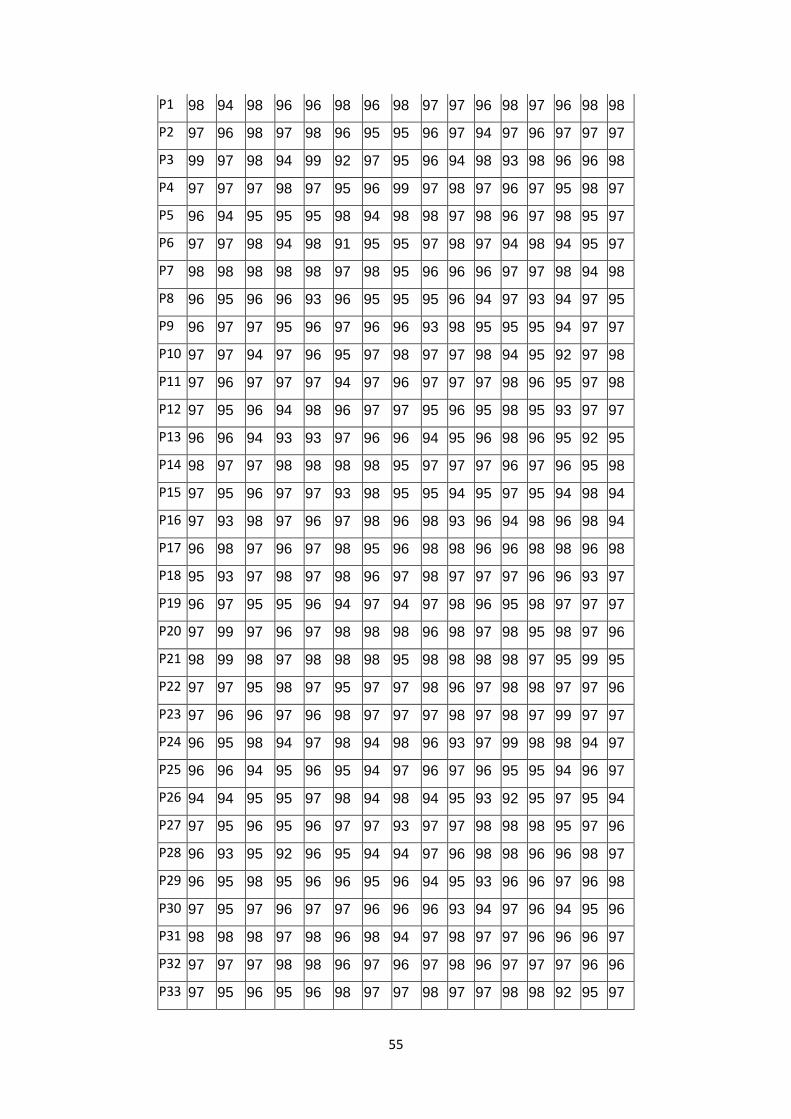
55

P1 98 94 98 96 96 98 96 98 97 97 96 98 97 96 98 98

P2 97 96 98 97 98 96 95 95 96 97 94 97 96 97 97 97

P3 99 97 98 94 99 92 97 95 96 94 98 93 98 96 96 98

P4 97 97 97 98 97 95 96 99 97 98 97 96 97 95 98 97

P5 96 94 95 95 95 98 94 98 98 97 98 96 97 98 95 97

P6 97 97 98 94 98 91 95 95 97 98 97 94 98 94 95 97

P7 98 98 98 98 98 97 98 95 96 96 96 97 97 98 94 98

P8 96 95 96 96 93 96 95 95 95 96 94 97 93 94 97 95

P9 96 97 97 95 96 97 96 96 93 98 95 95 95 94 97 97

P10 97 97 94 97 96 95 97 98 97 97 98 94 95 92 97 98

P11 97 96 97 97 97 94 97 96 97 97 97 98 96 95 97 98

P12 97 95 96 94 98 96 97 97 95 96 95 98 95 93 97 97

P13 96 96 94 93 93 97 96 96 94 95 96 98 96 95 92 95

P14 98 97 97 98 98 98 98 95 97 97 97 96 97 96 95 98

P15 97 95 96 97 97 93 98 95 95 94 95 97 95 94 98 94

P16 97 93 98 97 96 97 98 96 98 93 96 94 98 96 98 94

P17 96 98 97 96 97 98 95 96 98 98 96 96 98 98 96 98

P18 95 93 97 98 97 98 96 97 98 97 97 97 96 96 93 97

P19 96 97 95 95 96 94 97 94 97 98 96 95 98 97 97 97

P20 97 99 97 96 97 98 98 98 96 98 97 98 95 98 97 96

P21 98 99 98 97 98 98 98 95 98 98 98 98 97 95 99 95

P22 97 97 95 98 97 95 97 97 98 96 97 98 98 97 97 96

P23 97 96 96 97 96 98 97 97 97 98 97 98 97 99 97 97

P24 96 95 98 94 97 98 94 98 96 93 97 99 98 98 94 97

P25 96 96 94 95 96 95 94 97 96 97 96 95 95 94 96 97

P26 94 94 95 95 97 98 94 98 94 95 93 92 95 97 95 94

P27 97 95 96 95 96 97 97 93 97 97 98 98 98 95 97 96

P28 96 93 95 92 96 95 94 94 97 96 98 98 96 96 98 97

P29 96 95 98 95 96 96 95 96 94 95 93 96 96 97 96 98

P30 97 95 97 96 97 97 96 96 96 93 94 97 96 94 95 96

P31 98 98 98 97 98 96 98 94 97 98 97 97 96 96 96 97

P32 97 97 97 98 98 96 97 96 97 98 96 97 97 97 96 96

P33 97 95 96 95 96 98 97 97 98 97 97 98 98 92 95 97

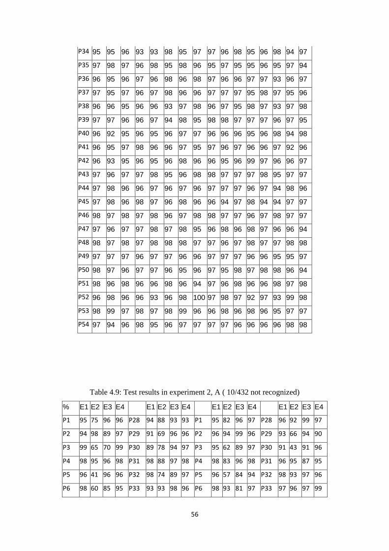
56

P34 95 95 96 93 93 98 95 97 97 96 98 95 96 98 94 97

P35 97 98 97 96 98 95 98 96 95 97 95 95 96 95 97 94

P36 96 95 96 97 96 98 96 98 97 96 96 97 97 93 96 97

P37 97 95 97 96 97 98 96 96 97 97 97 95 98 97 95 96

P38 96 96 95 96 96 93 97 98 96 97 95 98 97 93 97 98

P39 97 97 96 96 97 94 98 95 98 98 97 97 97 96 97 95

P40 96 92 95 96 95 96 97 97 96 96 96 95 96 98 94 98

P41 96 95 97 98 96 96 97 95 97 96 97 96 96 97 92 96

P42 96 93 95 96 95 96 98 96 96 95 96 99 97 96 96 97

P43 97 96 97 97 98 95 96 98 98 97 97 97 98 95 97 97

P44 97 98 96 96 97 96 97 96 97 97 97 96 97 94 98 96

P45 97 98 96 98 97 96 98 96 96 94 97 98 94 94 97 97

P46 98 97 98 97 98 96 97 98 98 97 97 96 97 98 97 97

P47 97 96 97 97 98 97 98 95 96 98 96 98 97 96 96 94

P48 98 97 98 97 98 98 98 97 97 96 97 98 97 97 98 98

P49 97 97 97 96 97 97 96 96 97 97 97 96 96 95 95 97

P50 98 97 96 97 97 96 95 96 97 95 98 97 98 98 96 94

P51 98 96 98 96 96 98 96 94 97 96 98 96 96 98 97 98

P52 96 98 96 96 93 96 98 100 97 98 97 92 97 93 99 98

P53 98 99 97 98 97 98 99 96 96 98 96 98 96 95 97 97

P54 97 94 96 98 95 96 97 97 97 97 96 96 96 96 98 98

Table 4.9: Test results in experiment 2, A ( 10/432 not recognized)

% E1 E2 E3 E4 E1 E2 E3 E4 E1 E2 E3 E4 E1 E2 E3 E4

P1 95 75 96 96 P28 94 88 93 93 P1 95 82 96 97 P28 96 92 99 97

P2 94 98 89 97 P29 91 69 96 96 P2 96 94 99 96 P29 93 66 94 90

P3 99 65 70 99 P30 89 78 94 97 P3 95 62 89 97 P30 91 43 91 96

P4 98 95 96 98 P31 98 88 97 98 P4 98 83 96 98 P31 96 95 87 95

P5 96 41 96 96 P32 98 74 89 97 P5 96 57 84 94 P32 98 93 97 96

P6 98 60 85 95 P33 93 93 98 96 P6 98 93 81 97 P33 97 96 97 99

57

P7 98 95 99 97 P34 95 80 99 95 P7 96 84 89 97 P34 94 76 89 95

P8 95 27 96 91 P35 98 90 96 97 P8 94 72 57 93 P35 97 24 96 96

P9 96 84 69 92 P36 90 75 93 96 P9 96 70 87 91 P36 93 77 94 96

P10 97 95 95 94 P37 96 87 94 97 P10 96 82 52 95 P37 97 95 97 97

P11 96 94 86 97 P38 98 59 89 94 P11 97 93 90 95 P38 94 39 97 95

P12 99 60 60 96 P39 95 82 96 97 P12 96 78 82 93 P39 97 67 93 97

P13 93 61 96 94 P40 89 77 97 96 P13 95 69 33 96 P40 93 28 98 97

P14 98 98 94 98 P41 97 88 96 96 P14 96 54 93 97 P41 93 74 96 97

P15 97 83 87 95 P42 96 79 98 97 P15 96 78 96 94 P42 96 70 95 97

P16 95 89 96 99 P43 94 81 96 98 P16 96 98 75 93 P43 96 95 94 97

P17 94 58 98 98 P44 98 77 87 96 P17 97 69 88 98 P44 97 36 78 97

P18 94 82 98 93 P45 98 87 95 97 P18 93 88 93 98 P45 96 81 81 96

P19 96 65 98 97 P46 97 82 94 98 P19 95 92 96 97 P46 97 80 94 98

P20 99 94 94 98 P47 98 77 96 97 P20 97 95 97 95 P47 95 85 84 96

P21 99 88 93 96 P48 98 90 96 98 P21 98 53 96 97 P48 97 83 91 97

P22 96 72 83 97 P49 97 59 93 98 P22 97 79 90 97 P49 93 91 76 98

P23 97 60 84 97 P50 92 95 79 98 P23 98 97 97 97 P50 89 80 93 93

P24 92 73 83 97 P51 98 87 86 97 P24 97 62 97 95 P51 96 83 81 94

P25 96 22 94 96 P52 98 62 76 95 P25 97 91 99 95 P52 99 92 97 97

P26 90 90 90 97 P53 99 91 96 98 P26 96 91 80 93 P53 97 82 96 95

P27 94 67 96 97 P54 93 48 83 96 P27 97 66 95 97 P54 98 90 90 96

Table 4.10: Test results of experiment2, B (59/432 Not recognized th=50%)

% E1 E2 E3 E4

E1 E2 E3 E4

E1 E2 E3 E4

E1 E2 E3 E4

P1 94 13 92 97 P28 92 51 85 95 P1 95 38 95 96 P28 94 77 78 96

P2 96 96 97 94 P29 65 73 71 95 P2 89 95 95 95 P29 95 36 89 95

P3 99 19 81 98 P30 51 78 93 97 P3 95 5 65 93 P30 59 27 92 97

P4 99 28 96 97 P31 96 89 84 98 P4 93 58 96 98 P31 90 68 90 97

P5 93 8 97 93 P32 99 50 76 96 P5 92 72 95 97 P32 93 47 95 96

P6 95 60 91 95 P33 95 12 97 97 P6 97 54 26 95 P33 96 90 97 98

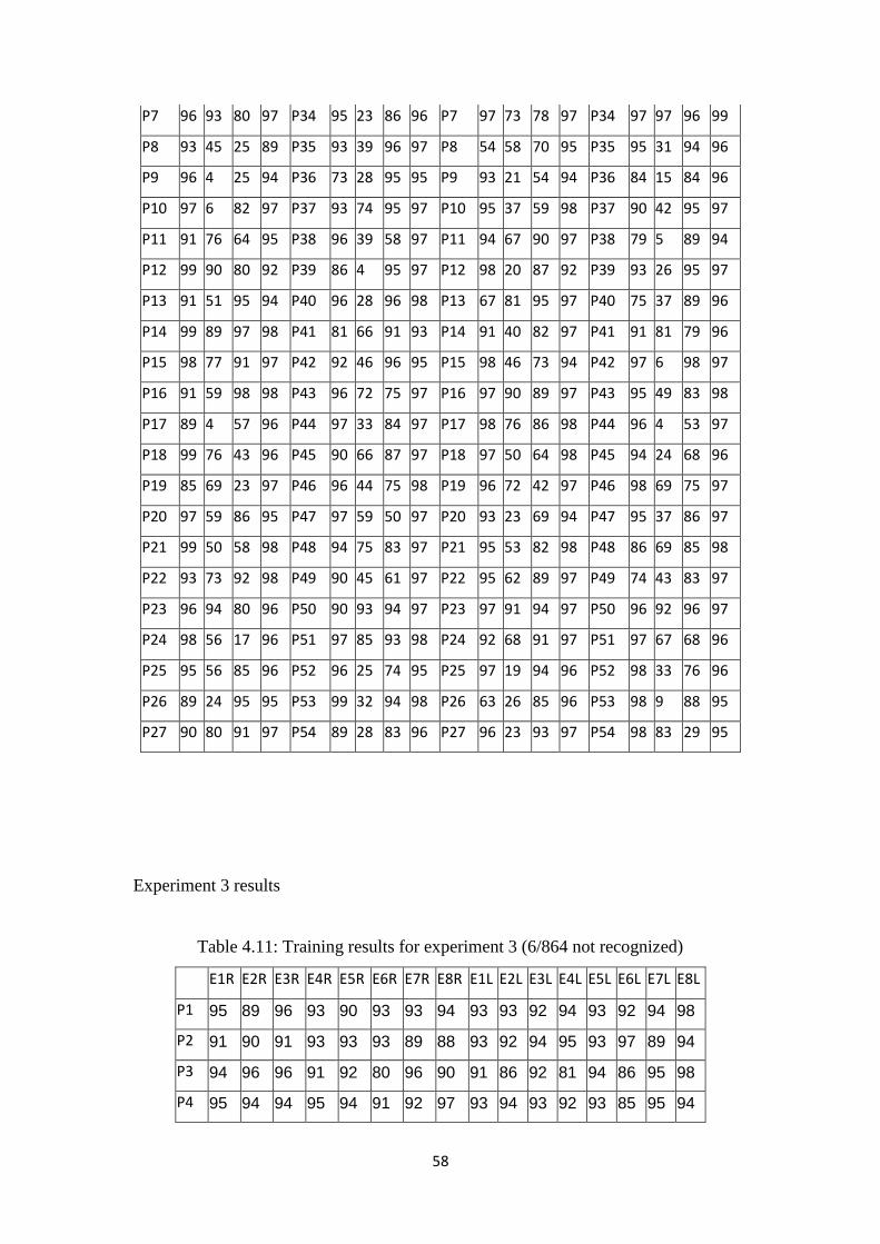
58

P7 96 93 80 97 P34 95 23 86 96 P7 97 73 78 97 P34 97 97 96 99

P8 93 45 25 89 P35 93 39 96 97 P8 54 58 70 95 P35 95 31 94 96

P9 96 4 25 94 P36 73 28 95 95 P9 93 21 54 94 P36 84 15 84 96

P10 97 6 82 97 P37 93 74 95 97 P10 95 37 59 98 P37 90 42 95 97

P11 91 76 64 95 P38 96 39 58 97 P11 94 67 90 97 P38 79 5 89 94

P12 99 90 80 92 P39 86 4 95 97 P12 98 20 87 92 P39 93 26 95 97

P13 91 51 95 94 P40 96 28 96 98 P13 67 81 95 97 P40 75 37 89 96

P14 99 89 97 98 P41 81 66 91 93 P14 91 40 82 97 P41 91 81 79 96

P15 98 77 91 97 P42 92 46 96 95 P15 98 46 73 94 P42 97 6 98 97

P16 91 59 98 98 P43 96 72 75 97 P16 97 90 89 97 P43 95 49 83 98

P17 89 4 57 96 P44 97 33 84 97 P17 98 76 86 98 P44 96 4 53 97

P18 99 76 43 96 P45 90 66 87 97 P18 97 50 64 98 P45 94 24 68 96

P19 85 69 23 97 P46 96 44 75 98 P19 96 72 42 97 P46 98 69 75 97

P20 97 59 86 95 P47 97 59 50 97 P20 93 23 69 94 P47 95 37 86 97

P21 99 50 58 98 P48 94 75 83 97 P21 95 53 82 98 P48 86 69 85 98

P22 93 73 92 98 P49 90 45 61 97 P22 95 62 89 97 P49 74 43 83 97

P23 96 94 80 96 P50 90 93 94 97 P23 97 91 94 97 P50 96 92 96 97

P24 98 56 17 96 P51 97 85 93 98 P24 92 68 91 97 P51 97 67 68 96

P25 95 56 85 96 P52 96 25 74 95 P25 97 19 94 96 P52 98 33 76 96

P26 89 24 95 95 P53 99 32 94 98 P26 63 26 85 96 P53 98 9 88 95

P27 90 80 91 97 P54 89 28 83 96 P27 96 23 93 97 P54 98 83 29 95

Experiment 3 results

Table 4.11: Training results for experiment 3 (6/864 not recognized)

E1R E2R E3R E4R E5R E6R E7R E8R E1L E2L E3L E4L E5L E6L E7L E8L

P1 95 89 96 93 90 93 93 94 93 93 92 94 93 92 94 98

P2 91 90 91 93 93 93 89 88 93 92 94 95 93 97 89 94

P3 94 96 96 91 92 80 96 90 91 86 92 81 94 86 95 98

P4 95 94 94 95 94 91 92 97 93 94 93 92 93 85 95 94

59

P5 87 89 85 86 82 94 89 95 91 91 92 86 89 92 93 96

P6 87 91 88 85 86 80 73 84 91 92 93 80 91 84 91 88

P7 94 97 96 91 94 95 95 91 90 90 91 92 90 85 87 93

P8 92 93 91 90 89 92 92 81 90 91 78 88 83 91 88 91

P9 87 94 89 85 87 94 90 89 87 94 88 87 87 81 95 75

P10 92 94 88 93 90 90 93 89 92 95 95 88 90 81 93 92

P11 92 92 91 93 92 88 89 84 92 93 93 91 91 92 94 94

P12 93 90 87 87 92 87 94 96 87 93 85 90 85 83 95 92

P13 86 77 85 80 76 94 89 82 82 83 83 94 82 94 84 84

P14 93 93 94 94 94 92 93 92 92 88 94 93 92 90 94 96

P15 92 88 93 88 93 91 91 85 88 85 88 94 86 84 95 86

P16 90 90 95 87 90 90 93 92 95 79 93 86 96 95 95 86

P17 90 92 90 89 89 90 95 93 92 93 92 86 93 94 92 89

P18 91 87 92 95 93 92 91 94 91 88 95 92 91 90 92 97

P19 93 95 91 88 89 84 86 89 94 94 93 82 95 96 95 94

P20 92 96 93 89 93 93 96 94 90 91 91 92 88 96 94 92

P21 95 97 95 94 95 91 97 83 95 95 94 92 94 90 96 87

P22 92 92 91 95 93 91 95 87 94 94 92 92 93 89 87 96

P23 92 93 94 93 92 92 94 89 95 95 96 95 93 94 95 91

P24 89 87 93 89 94 93 83 89 90 82 91 97 92 93 82 96

P25 85 86 78 83 82 81 76 85 88 92 86 84 89 87 85 73

P26 90 79 89 88 89 94 88 91 86 81 84 89 86 91 79 80

P27 93 91 88 82 93 87 93 88 94 95 95 95 95 88 91 92

P28 87 85 83 80 86 88 84 87 92 88 93 91 93 91 93 92

P29 88 83 91 89 90 88 88 92 85 86 84 87 84 87 93 95

P30 90 89 92 91 90 87 89 93 89 83 87 92 88 70 87 91

P31 94 95 93 94 94 90 97 90 93 93 94 94 89 94 93 92

P32 93 94 93 94 94 91 93 96 94 95 92 90 95 90 94 90

P33 93 91 90 85 92 94 93 92 93 89 90 94 95 84 89 97

P34 85 85 88 83 80 89 89 91 91 90 94 90 90 95 87 86

P35 90 90 89 93 93 83 91 97 89 90 89 91 87 89 86 93

P36 93 85 92 89 89 91 88 87 92 88 91 90 92 82 87 92

P37 94 88 92 93 94 92 88 89 93 93 91 93 95 96 92 91

60

P38 89 89 86 92 88 89 90 92 92 94 91 95 95 73 94 90

P39 90 94 88 87 91 91 91 89 92 95 91 92 93 88 94 90

P40 90 87 88 89 90 91 88 95 87 90 87 92 88 88 91 96

P41 91 90 94 92 89 90 90 93 92 91 90 91 92 89 84 88

P42 88 91 92 86 89 84 94 88 91 93 89 92 89 95 94 93

P43 95 94 94 92 94 92 91 95 95 93 95 93 95 93 94 94

P44 93 91 90 92 93 92 92 89 92 94 90 93 92 92 94 92

P45 93 92 92 94 94 91 94 93 91 82 90 92 91 88 94 86

P46 95 96 95 91 96 91 97 95 94 92 93 89 92 95 91 92

P47 92 91 93 94 94 90 94 96 91 92 91 91 89 88 93 94

P48 96 94 95 94 96 96 96 94 94 91 95 94 93 95 91 95

P49 92 93 90 89 93 92 89 88 94 94 94 85 94 90 94 86

P50 93 87 86 93 92 93 88 90 94 87 95 92 91 96 85 93

P51 93 90 93 92 91 94 90 91 93 92 94 85 93 95 94 94

P52 90 92 91 93 86 88 95 97 90 91 88 86 88 82 94 95

P53 95 96 93 95 94 93 96 92 93 94 91 94 92 91 94 89

P54 91 86 89 91 89 94 91 89 94 91 93 92 92 91 94 96

Table 4.12: Test results, A (24/432 Not recognized, threshold = 0.5)

% E1 E2 E3 E4 E1 E2 E3 E4 E1 E2 E3 E4 E1 E2 E3 E4

P1 90 73 84 95 P28 82 62 91 81 P1 92 67 93 94 P28 86 96 91 92

P2 90 97 85 93 P29 83 57 78 89 P2 89 79 95 92 P29 78 56 88 79

P3 97 51 69 96 P30 87 75 78 89 P3 91 64 70 95 P30 82 69 88 89

P4 94 73 96 95 P31 95 94 92 94 P4 93 68 94 93 P31 90 48 78 86

P5 92 53 93 89 P32 95 90 87 93 P5 89 49 84 87 P32 95 83 83 93

P6 89 28 63 82 P33 83 92 89 90 P6 92 38 81 90 P33 92 95 95 95

P7 95 81 84 92 P34 79 86 84 84 P7 87 85 87 94 P34 89 91 82 93

P8 88 24 89 90 P35 94 58 90 88 P8 79 29 53 88 P35 91 40 81 89

P9 88 32 24 74 P36 82 67 89 91 P9 91 48 59 89 P36 83 76 87 93

P10 94 52 89 85 P37 92 85 93 94 P10 94 95 49 93 P37 89 76 93 93

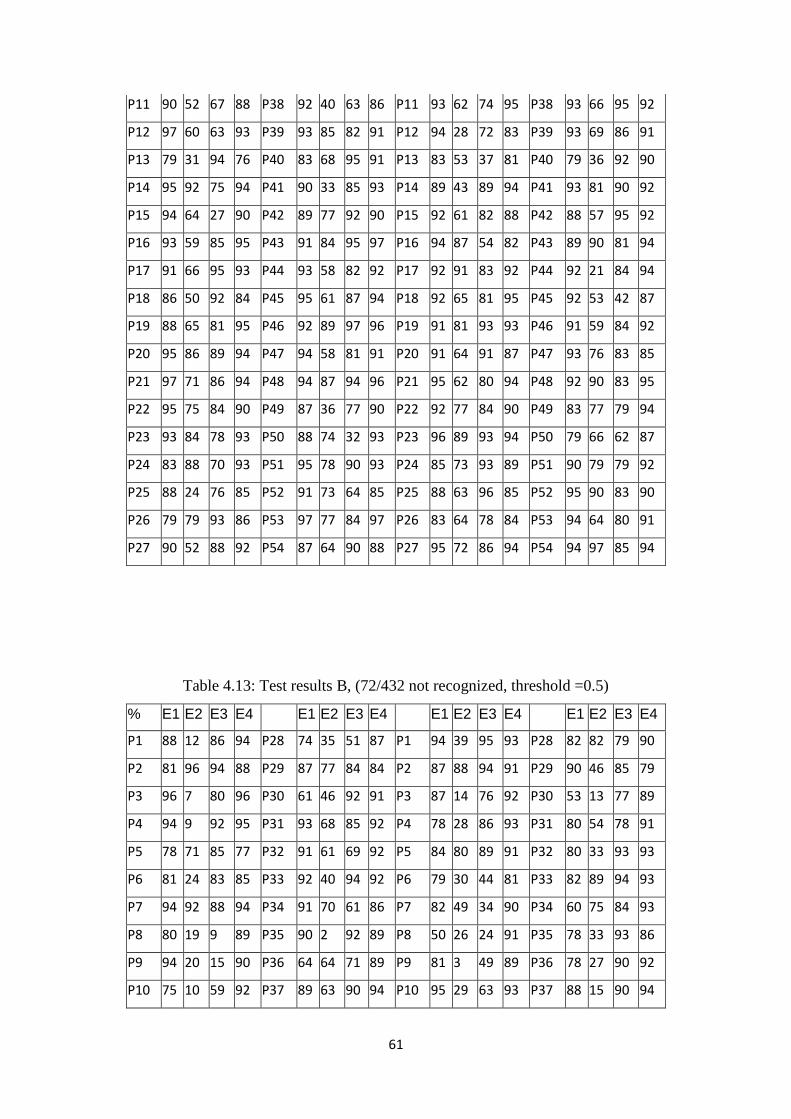
61

P11 90 52 67 88 P38 92 40 63 86 P11 93 62 74 95 P38 93 66 95 92

P12 97 60 63 93 P39 93 85 82 91 P12 94 28 72 83 P39 93 69 86 91

P13 79 31 94 76 P40 83 68 95 91 P13 83 53 37 81 P40 79 36 92 90

P14 95 92 75 94 P41 90 33 85 93 P14 89 43 89 94 P41 93 81 90 92

P15 94 64 27 90 P42 89 77 92 90 P15 92 61 82 88 P42 88 57 95 92

P16 93 59 85 95 P43 91 84 95 97 P16 94 87 54 82 P43 89 90 81 94

P17 91 66 95 93 P44 93 58 82 92 P17 92 91 83 92 P44 92 21 84 94

P18 86 50 92 84 P45 95 61 87 94 P18 92 65 81 95 P45 92 53 42 87

P19 88 65 81 95 P46 92 89 97 96 P19 91 81 93 93 P46 91 59 84 92

P20 95 86 89 94 P47 94 58 81 91 P20 91 64 91 87 P47 93 76 83 85

P21 97 71 86 94 P48 94 87 94 96 P21 95 62 80 94 P48 92 90 83 95

P22 95 75 84 90 P49 87 36 77 90 P22 92 77 84 90 P49 83 77 79 94

P23 93 84 78 93 P50 88 74 32 93 P23 96 89 93 94 P50 79 66 62 87

P24 83 88 70 93 P51 95 78 90 93 P24 85 73 93 89 P51 90 79 79 92

P25 88 24 76 85 P52 91 73 64 85 P25 88 63 96 85 P52 95 90 83 90

P26 79 79 93 86 P53 97 77 84 97 P26 83 64 78 84 P53 94 64 80 91

P27 90 52 88 92 P54 87 64 90 88 P27 95 72 86 94 P54 94 97 85 94

Table 4.13: Test results B, (72/432 not recognized, threshold =0.5)

% E1 E2 E3 E4

E1 E2 E3 E4

E1 E2 E3 E4

E1 E2 E3 E4

P1 88 12 86 94 P28 74 35 51 87 P1 94 39 95 93 P28 82 82 79 90

P2 81 96 94 88 P29 87 77 84 84 P2 87 88 94 91 P29 90 46 85 79

P3 96 7 80 96 P30 61 46 92 91 P3 87 14 76 92 P30 53 13 77 89

P4 94 9 92 95 P31 93 68 85 92 P4 78 28 86 93 P31 80 54 78 91

P5 78 71 85 77 P32 91 61 69 92 P5 84 80 89 91 P32 80 33 93 93

P6 81 24 83 85 P33 92 40 94 92 P6 79 30 44 81 P33 82 89 94 93

P7 94 92 88 94 P34 91 70 61 86 P7 82 49 34 90 P34 60 75 84 93

P8 80 19 9 89 P35 90 2 92 89 P8 50 26 24 91 P35 78 33 93 86

P9 94 20 15 90 P36 64 64 71 89 P9 81 3 49 89 P36 78 27 90 92

P10 75 10 59 92 P37 89 63 90 94 P10 95 29 63 93 P37 88 15 90 94

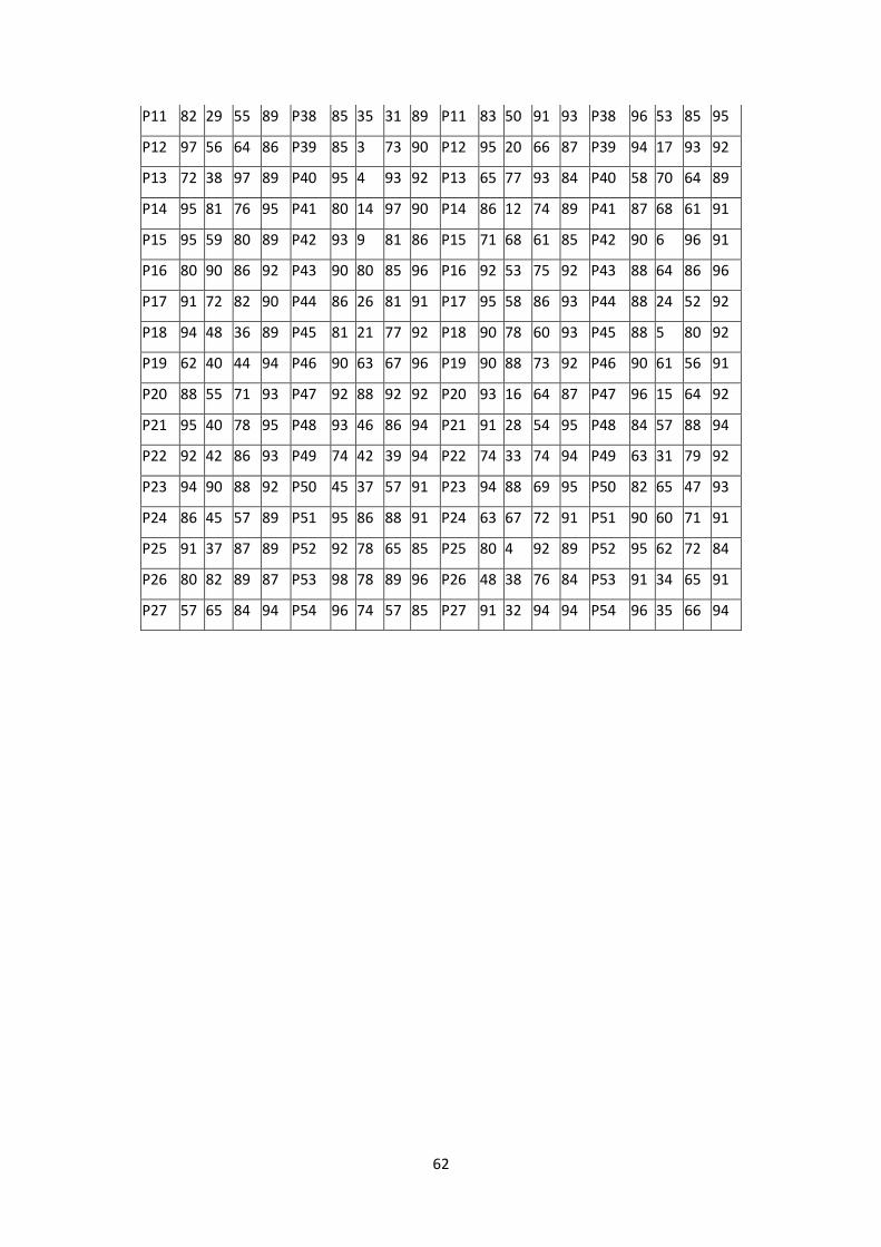
62

P11 82 29 55 89 P38 85 35 31 89 P11 83 50 91 93 P38 96 53 85 95

P12 97 56 64 86 P39 85 3 73 90 P12 95 20 66 87 P39 94 17 93 92

P13 72 38 97 89 P40 95 4 93 92 P13 65 77 93 84 P40 58 70 64 89

P14 95 81 76 95 P41 80 14 97 90 P14 86 12 74 89 P41 87 68 61 91

P15 95 59 80 89 P42 93 9 81 86 P15 71 68 61 85 P42 90 6 96 91

P16 80 90 86 92 P43 90 80 85 96 P16 92 53 75 92 P43 88 64 86 96

P17 91 72 82 90 P44 86 26 81 91 P17 95 58 86 93 P44 88 24 52 92

P18 94 48 36 89 P45 81 21 77 92 P18 90 78 60 93 P45 88 5 80 92

P19 62 40 44 94 P46 90 63 67 96 P19 90 88 73 92 P46 90 61 56 91

P20 88 55 71 93 P47 92 88 92 92 P20 93 16 64 87 P47 96 15 64 92

P21 95 40 78 95 P48 93 46 86 94 P21 91 28 54 95 P48 84 57 88 94

P22 92 42 86 93 P49 74 42 39 94 P22 74 33 74 94 P49 63 31 79 92

P23 94 90 88 92 P50 45 37 57 91 P23 94 88 69 95 P50 82 65 47 93

P24 86 45 57 89 P51 95 86 88 91 P24 63 67 72 91 P51 90 60 71 91

P25 91 37 87 89 P52 92 78 65 85 P25 80 4 92 89 P52 95 62 72 84

P26 80 82 89 87 P53 98 78 89 96 P26 48 38 76 84 P53 91 34 65 91

P27 57 65 84 94 P54 96 74 57 85 P27 91 32 94 94 P54 96 35 66 94