Chapter One

Ordinary Differential Equations of Order One

1. Introduction to Ordinary Differential EquationsThe first question one might ask in a course in differential equations is ”what are

differential equations and where do they come from?” To begin to answer that question,consider the following example. A cup of hot coffee is brought into a room and set on thetable. We know from experience that the coffee will begin to cool and continue cooling untilthe temperature of the coffee is reduced to the temperature of the room. We are going toappeal to known physical laws, namely Newton’s law of cooling, and translate theapplication of that law to the cooling cup of coffee into mathematical terms. Thismathematical expression of Newton’s law as it applies to the coffee will be a differentialequation whose solution will allow us to predict the temperature of the coffee at every timeduring the process of cooling.

In other words, a differential equation often arises when we translate into mathematicalterms the physical laws that describe the behavior of some physical system. Solving thedifferential equation allows us to understand and to predict the behavior of the physicalsystem. Of course not all differential equations arise in this way, but in any case the solutionof a differential equation is not just a number as is the case when we solve an algebraicequation. The solution of a differential equation is a function having the property that when itis substituted into the differential equation, the equation is identically satisfied for all valuesof the independent variable. But let us demonstrate what all this means with some concreteexamples.

1.1 A Simple Mathematical ModelTo describe the situation of the cooling cup of coffee analytically, we first define a

function T�t�, whose value at each positive value of t is the temperature of the coffee at timet. We make the simplifying assumption that the temperature is the same at every point inthe cup;i.e., that T�t� depends only on t. We define t � 0 to be the initial time at which thecoffee was set on the table and we assume t increases from zero. The time t is referred toas the independent variable in the problem, and T�t� is the dependent variable (becauseT depends on t�. If we denote the temperature of the room to be the constant TR, (anothersimplifying assumption) then we can begin an analytic description of the cooling process forthe coffee. For example, we can say that:

� if T�t� � TR then T�t� decreases i. e. , T��t� � 0

� if T�t� � TR then T�t� increases i. e. , T��t� � 0

Then we might be inclined to assume that T��t� and �T�t� � TR� are related, in fact, wemight assume that T��t� is proportional to �T�t� � TR�; i.e., the temperature changes rapidlywhen the difference between the temperature of the coffee and the temperature of the roomis large, and it changes more slowly as this difference decreases. This would be expressedas follows

T��t� � �k �T�t� � TR� �1�

1

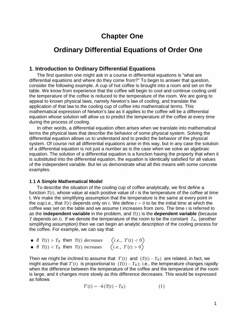
where k denotes a positive constant of proportionality and the negative sign appears so thatT��t� is negative when �T�t� � TR� is positive in accordance with our previous observations.Then (1) is an example of a differential equation. It is called this because it is an equationinvolving an unknown function T�t� and also its derivative T��t�. More precisely, (1) is calledan ordinary differential equation because the derivative which appears is an ordinaryderivative (as opposed to a partial derivative which occurs when the unknown functiondepends on more than one independent variable). In addition, we say that (1) is a firstorder equation because there are no derivatives of order more than one, and finally we saythat (1) is a linear first order ordinary differential equation (but we will wait until later toexplain the meaning of the term, ”linear”).

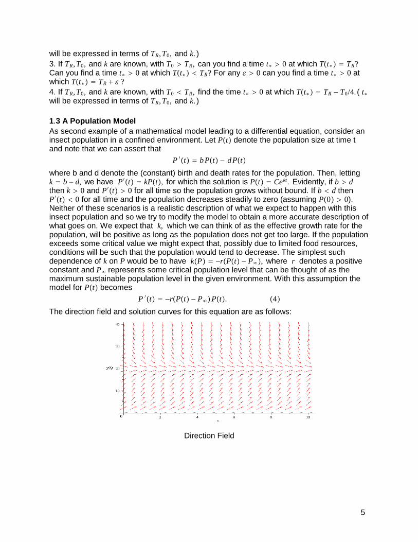
Direction FieldWe can now think of the equation (1) as a mathematical model for the physical process of acooling cup of coffee.

1.2 The Notion of a SolutionOnce we have the mathematical model in the form of a differential equation, it will be ouraim to solve the equation and to use the solution to predict and understand the physicalsystem. Of course we need to understand what is meant by a solution for the equation. Onemeaning for the term solution might be a ”direction field” for the equation (1). Note that theequation defines a value of the derivative T��t� at each point in the T-t plane. Then at eachpoint �t, T� in the plane, we could imagine a small segment whose slope equals T��t�. Apicture of this would look like the figure above.

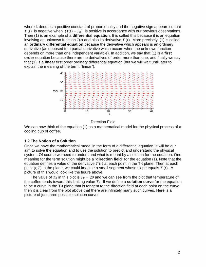
The value of TR in this plot is TR � 20 and we can see from the plot that temperature ofthe coffee tends toward this limiting value TR. If we define a solution curve for the equationto be a curve in the T-t plane that is tangent to the direction field at each point on the curve,then it is clear from the plot above that there are infinitely many such curves. Here is apicture of just three possible solution curves

2

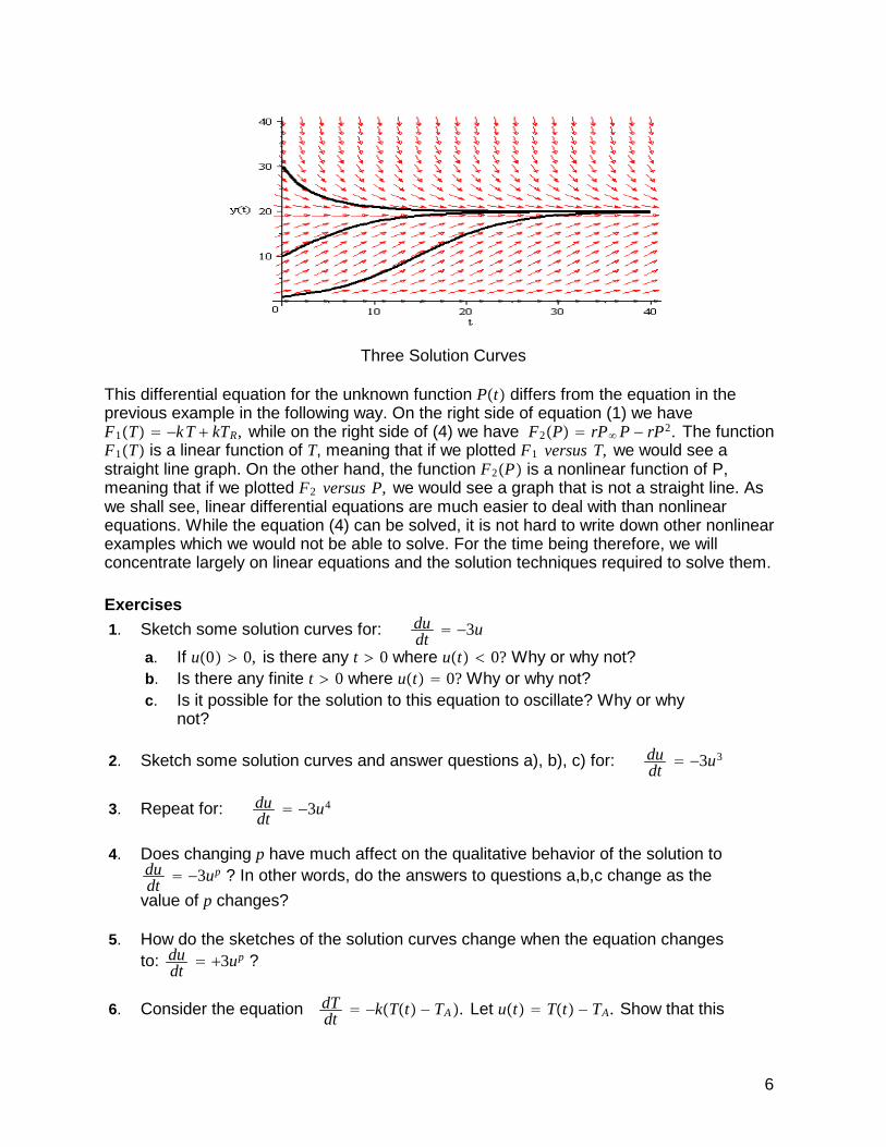
Three Solution CurvesEvidently the differential equation (1) has an infinite family of solution curves, each of whichis a possible description of how the temperature of the coffee varies with time. Notice thatthe three solution curves in the figure above correspond to different "initial values". That is,the uppermost curve starts from the value 50 at t � 0, while the other two curves begin fromthe values 30 and 10, respectively. Since 50 and 30 are greater than TR � 20, these curvesindicate that the temperatures decrease gradually to TR, while the curve that begins fromthe value 10 gradually increases to TR.

To better understand what this means, we can try to find the equations for the solutioncurves by doing the following. We can write (1) in the form

ddt

T�t� � �k�T�t� � TR�

and then rewrite it as

� dTT�t� � TR

� �k � dt.

Since

� dt � t � C0

and � dTT�t� � TR

� ln�T�t� � TR� � C1,

we find

ln�T�t� � TR� � C1 � �k�t � C0�

or, equivalently

ln�T�t� � TR� � �kt � C2.

Here C0, C1, C2 all are arbitrary constants (you can solve for C2 in terms of C0, C1if youwant to but C2 is still just an arbitrary constant). What we have at this point is an implicitfunctional relation between T and t. In some cases it will not be possible to resolve thisexpression to obtain an explicit formula for T in terms of t, but here we note that

e ln�T�t��TR � � e�kt�C2

� e�kteC2

� C3e�kt

3

and since e ln�T�t��TR � � T�t� � TR, we obtain,

T�t� � TR � C3e�kt. �2�

The constant C3 is another arbitrary constant of integration and for each choice of thisconstant, �2� is a solution of the equation �1�. It is also true that for each choice of theconstant, �2� is the equation of one of the solution curves for (1). We refer to �2� as a1-parameter family of solutions for (1) where C3 is the parameter that distinguishes betweenthe infinitely many family members. Evidently an equation like (1) has an infinite family ofsolutions.

Finally, suppose that the initial temperature of the coffee is known; i.e., supposeT�0� � T0 � TR where T0 is given. Then, according to (2)

T�0� � TR � C3e�k0

� TR � C3

� T0,

hence C3 � T0 � TR, and

T�t� � TR � �T0 � TR�e�kt. �3�

This is the unique solution that satisfies (1) as well as the initial condition, T�0� � T0.Evidently, the problem consisting of the differential equation (1) and the initial condition hasa unique solution. In the picture of solution curves seen above, the upper curve is thesolution curve corresponding to T0 � 50, while the lower curves correspond to T0 � 30 andT0 � 10, respectively. Here TR � 20 so the upper two curves decrease toward TR while thelowest curve increases asymptotically towards TR.

Once the solution is known, then it may be used to analyze the physical system. Forexample, if the initial temperature of the coffee was unknown but the temperature of thecoffee at some later time, say t � 2, is known to be equal to T�2� � T2, then the initialtemperature can be found. If we use (2) to write

T�2� � TR � C3e�2k � T2,

then

C3e�2k � T2 � TR

and

C3 � �T2 � TR�e2k.

Now we use this expression for C3 in (2) to obtainT�t� � TR � �T2 � TR�e2ke�kt

� TR � �T2 � TR�e�k�t�2�

from which it follows that the initial temperature of the coffee is equal to,

T�0� � TR � �T2 � TR�e2k.

We are assuming here that the constant k is a given positive constant.

Exercises-1. If the constant k is unknown, but it is given that T�0� � T0, T�2� � T2 � T0, then use thisinformation to find k in terms of TR, T0, and T2 .2. If TR, T0, and k are known, with T0 � TR, find the time t� � 0 at which T�t�� � TR � T0/2. ( t�

4

will be expressed in terms of TR, T0, and k. )3. If TR, T0, and k are known, with T0 � TR, can you find a time t� � 0 at which T�t�� � TR?Can you find a time t� � 0 at which T�t�� � TR? For any � � 0 can you find a time t� � 0 atwhich T�t�� � TR � � ?4. If TR, T0, and k are known, with T0 � TR, find the time t� � 0 at which T�t�� � TR � T0/4. ( t�will be expressed in terms of TR, T0, and k. )

1.3 A Population ModelAs second example of a mathematical model leading to a differential equation, consider aninsect population in a confined environment. Let P�t� denote the population size at time tand note that we can assert that

P ��t� � b P�t� � d P�t�

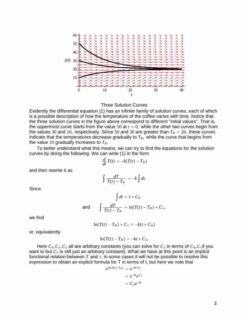
where b and d denote the (constant) birth and death rates for the population. Then, lettingk � b � d, we have P ��t� � kP�t�, for which the solution is P�t� � Cekt. Evidently, if b � dthen k � 0 and P ��t� � 0 for all time so the population grows without bound. If b � d thenP ��t� � 0 for all time and the population decreases steadily to zero (assuming P�0� � 0).Neither of these scenarios is a realistic description of what we expect to happen with thisinsect population and so we try to modify the model to obtain a more accurate description ofwhat goes on. We expect that k, which we can think of as the effective growth rate for thepopulation, will be positive as long as the population does not get too large. If the populationexceeds some critical value we might expect that, possibly due to limited food resources,conditions will be such that the population would tend to decrease. The simplest suchdependence of k on P would be to have k�P� � �r�P�t� � P��, where r denotes a positiveconstant and P� represents some critical population level that can be thought of as themaximum sustainable population level in the given environment. With this assumption themodel for P�t� becomes

P ��t� � �r�P�t� � P��P�t�. �4�

The direction field and solution curves for this equation are as follows:

Direction Field

5

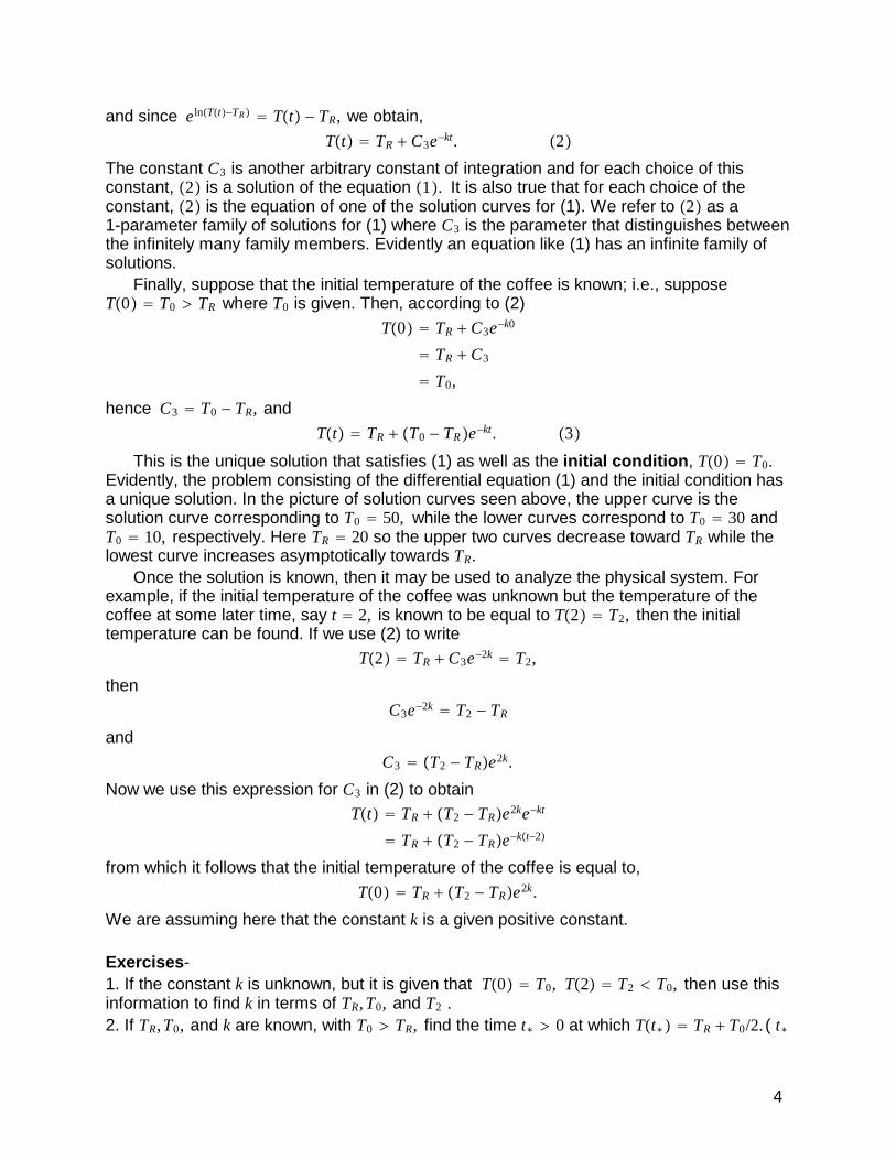
Three Solution Curves

This differential equation for the unknown function P�t� differs from the equation in theprevious example in the following way. On the right side of equation (1) we haveF1�T� � �k T � kTR, while on the right side of (4) we have F2�P� � rP� P � rP2. The functionF1�T� is a linear function of T, meaning that if we plotted F1 versus T, we would see astraight line graph. On the other hand, the function F2�P� is a nonlinear function of P,meaning that if we plotted F2 versus P, we would see a graph that is not a straight line. Aswe shall see, linear differential equations are much easier to deal with than nonlinearequations. While the equation (4) can be solved, it is not hard to write down other nonlinearexamples which we would not be able to solve. For the time being therefore, we willconcentrate largely on linear equations and the solution techniques required to solve them.

Exercises1. Sketch some solution curves for: du

dt� �3u

a. If u�0� � 0, is there any t � 0 where u�t� � 0? Why or why not?b. Is there any finite t � 0 where u�t� � 0? Why or why not?c. Is it possible for the solution to this equation to oscillate? Why or why

not?

2. Sketch some solution curves and answer questions a), b), c) for: dudt

� �3u3

3. Repeat for: dudt

� �3u4

4. Does changing p have much affect on the qualitative behavior of the solution todudt

� �3up ? In other words, do the answers to questions a,b,c change as the

value of p changes?

5. How do the sketches of the solution curves change when the equation changesto: du

dt� �3up ?

6. Consider the equation dTdt

� �k�T�t� � TA�. Let u�t� � T�t� � TA. Show that this

6

implies dudt

� �k u�t�.

7. If T�0� � TA � 100, then what is the value of u�0�? As t � �, what happens to thevalues of T�t� and u�t�?

8. Integrate to solve:

a. dudt

� �u�t�, u�0� � 5.

b. dudt

� �u2�t�, u�0� � 5.

2. Solution Methods For First Order Ordinary Differential EquationsWe are going to discuss a number of methods for constructing solutions for first orderordinary differential equations but our discussion will be confined to a few methods that canbe applied to the equations that occur most frequently in applications.

2.1 Separable equationsPerhaps the simplest case in which the solution can be constructed is when the differentialequation has the form

dydt

� P�y� Q�t�

We say the equation is separable and proceed to integrate by writing

� dyP�y�

� �Q�t�dt

and integrating. Note that it appears as if we are treating dydt

as if it is a fraction and crossmultiplying. In fact, what we are doing is the following:

�Q�t�dt � � 1P�y�

dydt

dt � � dyP�y�

Examples1. Consider the equation

dydt

� ty�t�.

Then

� dyy � � tdt.

Integrating the two sides of this last equation leads to,

ln y�t� � t2/2 � C1

and since exp�ln y�t�� � y�t�,

y�t� � C2e t2/2.

2. Sometimes the integration is more difficult as in the following equation,dydt

� �y�t��1 � y�t��

Then

7

� dyy�1 � y�

� �� dt

We must employ partial fractions to write1

y�1 � y�� 1

y � 1y � 1

.

Then

� dyy�1 � y�

� �� 1y � 1

y � 1�dy

� ln y � ln�y � 1�

� lny

y � 1� �t � C1.

Then, as in the previous example,y�t�

y�t� � 1� C2e�t

or

y�t� � C2e�t�y�t� � 1�.

These last two expressions are called "implicit solutions" since they do not give y�t� explicitlyas a function of t. After a little algebra, the explicit solution can be written as,

y�t� �C2e�t

C2e�t � 1.

ExercisesFind the general solution for each of the following equations by separating and integrating. Ifthere is an initial condition, find the unique solution to the initial value problem.

1. y ��t� �ty�t�

1 � y�t�2

2. y ��t� � �t � 1��y � 1�3. y ��t� � t �y2 � 4y � 3� y�0� � 1

4. y ��t� � t 1y � 2

y�0� � 2

5. �t2 � 1�y ��t� � 2t y�t�6. 2y ��t� � t y�t�3 y�1� � 17. y ��t� � 3t2 y�t� y�0� � 1

10

8. y ��t� � 3t2 y�t�2 y�0� � 110

9. y ��t� � e t�y

10. 2y ��t� � 1 � y�t�2

2.2 Exact EquationsAnother type of equation where constructing the solution is rather simple are the equationswhich take the form of an exact differential. To see what this means suppose F�t, y�t�� is asmooth function of two variables. Then the total differential of F is written,

dF � �F�t

dt � �F�y

dy.

8

Since F depends explicitly on both t and y, then any change in either t or y will contribute toa change in F. The total differential expresses the relationship between the changes in t andy and the corresponding change in F. If F is constant for all t and y then dF � 0 so it is clearthat the differential equation

�F�t

dt � �F�y

dy � 0 or �F�y

dydt

� � �F�t

is equivalent to F�t, y� � constant. In general, F�t, y� � C implicitly defines curves y � y�t�called level curves of the function F and these curves are then also the solution curves ofthe differential equation dF � 0.

For example, F�t, y� � yptq and dF � 0 leads to the equationqtq�1yp dt � pyp�1tq dy � 0

ordydt

� � qtq�1yp

pyp�1tq � � qypt

whose solution is yptq � C or y�t� � Ct�q/p.In a case like this, we say the differential equation is exact. In general, the equation

P�y, t�dy � Q�y, t�dt � 0

is exact if P � �F�y

and Q � �F�t

for some smooth function F�t, y�. If such an F exists

then it is necessary that

��t

�F�y

� ��y

�F�t

or

�P�t

��Q�y

.

If this last condition is satisfied then a function F�t, y� exists such that the solution curves ofthe equation are the so called "level curves" of F; i.e. the curves such that F�t, y� �constant.

For example, consider the differential equation

�2t � 2y�dy � �4t � 2y � 5�dt � 0.

Then

P�y, t� � 2t � 2y and �P�t

� 2,

Q�y, t� � �4t � 2y � 5 and�Q�y

� 2.

This tells us there exists a smooth F�t, y� for which

P � �F�y

� 2t � 2y

Q � �F�t

� ��4t � 2y � 5�

Integrating the first of these equalities with respect to y implies

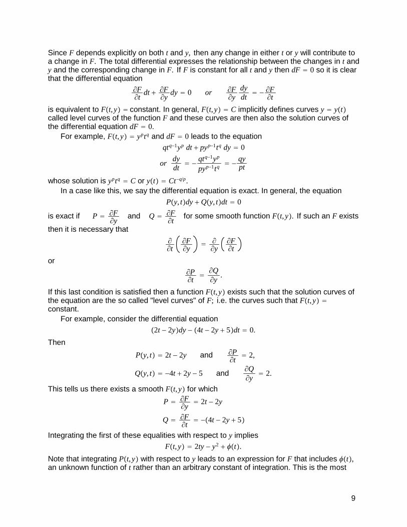
F�t, y� � 2ty � y2 � ��t�.

Note that integrating P�t, y� with respect to y leads to an expression for F that includes ��t�,an unknown function of t rather than an arbitrary constant of integration. This is the most

9

general antiderivative of P with respect the variable y. Similarly, integrating Q�t, y� withrespect to t leads to

F�t, y� � �2t2 � 2ty � 5t � ��y�,

which is the most general antiderivative of Q with respect to the variable t. By inspection, itwould appear from comparing the two results for F�t, y�, that ��t� � �5t � 2t2, and��y� � �y2.

A more rigorous approach is to use the first expression for F to compute�F�t

� Q

2y � ���t� � �4t � 2y � 5.

Then���t� � �4t � 5

and ��t� � �2t2 � 5t � C1.

Similarly, the second expression derived for F implies�F�y

� P

2t � ���y� � 2t � 2y

Then���y� � �2y,

or ��y� � �y2 � C2.

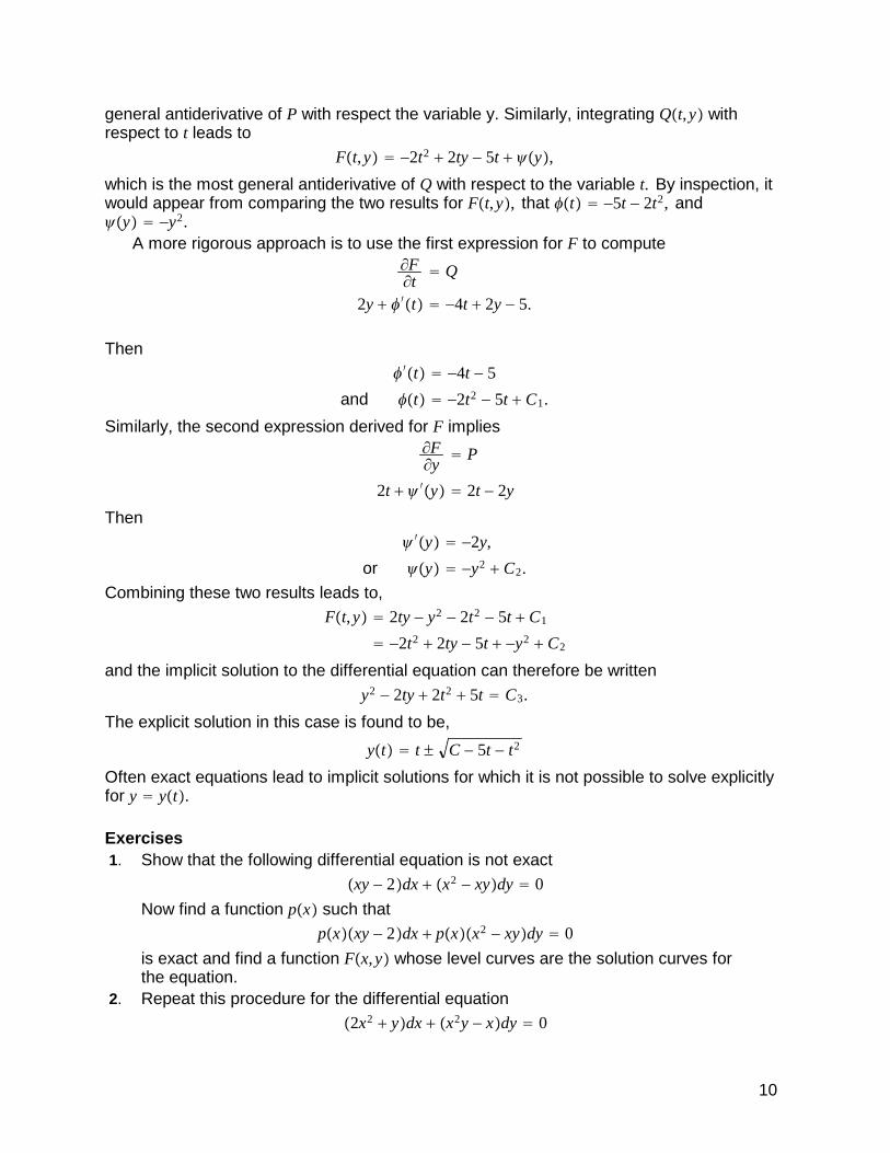
Combining these two results leads to,F�t, y� � 2ty � y2 � 2t2 � 5t � C1

� �2t2 � 2ty � 5t � �y2 � C2

and the implicit solution to the differential equation can therefore be written

y2 � 2ty � 2t2 � 5t � C3.

The explicit solution in this case is found to be,

y�t� � t � C � 5t � t2

Often exact equations lead to implicit solutions for which it is not possible to solve explicitlyfor y � y�t�.

Exercises1. Show that the following differential equation is not exact

�xy � 2�dx � �x2 � xy�dy � 0

Now find a function p�x� such thatp�x��xy � 2�dx � p�x��x2 � xy�dy � 0

is exact and find a function F�x, y� whose level curves are the solution curves forthe equation.

2. Repeat this procedure for the differential equation

�2x2 � y�dx � �x2y � x�dy � 0

10

3. Show that the following differential equation is not exact

y dx � �2x � yey�dy � 0

Now find a function q�y� such that

q�y� y dx � q�y��2x � yey�dy � 0

is exact and find a function F�x, y� whose level curves are the solution curves forthe equation.

4. Show thatdydt

�t3 � yy3 � t

is exact and solve.5. Show that

dydt

�y2 � yt

t2

is not exact butdydt

��y2 � yt�/y2t

t2/y2t�

1/t � 1/yt/y2

is exact. Solve this equation.

2.3 Linear EquationsLinear equations provide a mathematical description of a large number of physicalphenomena and are therefore an important class of differential equation. For example, thenonlinear problem

y ��t� � F�y�t�� y�0� � y0

can be approximated by the following linear problem,

y ��t� � F�y0� � F ��y0��y�t� � y0� y�0� � y0.

In general the behavior of solutions to linear equations is more restricted than the behaviorof solutions to nonlinear differential equations but the linear problem is usually easier tosolve.

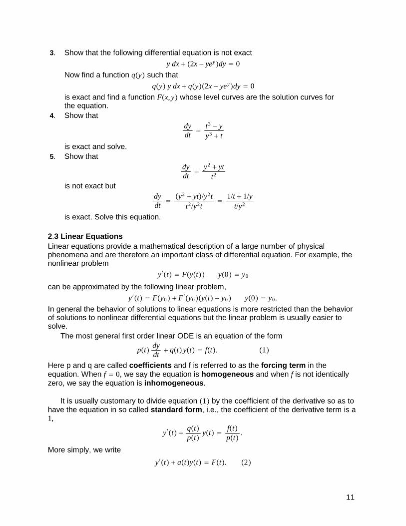
The most general first order linear ODE is an equation of the form

p�t�dydt

� q�t�y�t� � f�t�. �1�

Here p and q are called coefficients and f is referred to as the forcing term in theequation. When f � 0, we say the equation is homogeneous and when f is not identicallyzero, we say the equation is inhomogeneous.

It is usually customary to divide equation �1� by the coefficient of the derivative so as tohave the equation in so called standard form, i.e., the coefficient of the derivative term is a1,

y ��t� �q�t�p�t�

y�t� �f�t�p�t�

.

More simply, we write

y ��t� � a�t�y�t� � F�t�. �2�

11

If we introduce the notation

L�y�t�� � y ��t� � a�t�y�t�

then it is easy to see that for any constant, C, and any function y�t� having a derivative,L�Cy�t�� � �Cy�t�� � � a�t�Cy�t�

� C y ��t� � Ca�t�y�t�

� CL�y�t��

In the same way, it is clear thatL�y1�t� � y2�t�� � �y1�t� � y2�t�� � � a�t��y1�t� � y2�t��

� y1� �t� � a�t�y1�t� � y2

� �t� � a�t�y2�t�

� L�y1�t�� � L�y2�t��.

Combining these two results leads to the result that for all functions y1 and y2 and allconstants C1 and C2,

L�C1y1�t� � C2y2�t�� � C1L�y1�t�� � C2L�y2�t��.

This property is referred to as the property of linearity and L��� here is called a linearoperator. The differential equation L�y�t�� � F�t� is called a linear differential equation.Since the operator L involves no derivative of order higher than one, L is called a first orderlinear differential operator.

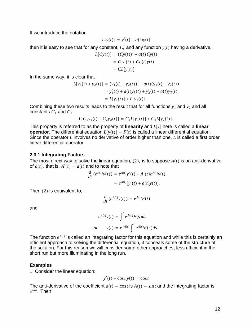
2.3.1 Integrating FactorsThe most direct way to solve the linear equation, �2�, is to suppose A�t� is an anti-derivativeof a�t�, that is, A ��t� � a�t� and to note that

ddt

�eA�t�y�t�� � eA�t�y ��t� � A ��t�eA�t�y�t�

� eA�t��y ��t� � a�t�y�t��.

Then �2� is equivalent to,ddt

�eA�t�y�t�� � eA�t�F�t�

and

eA�t�y�t� � � teA�s�F�s�ds

or y�t� � e�A�t� � teA�s�F�s�ds.

The function eA�t� is called an integrating factor for this equation and while this is certainly anefficient approach to solving the differential equation, it conceals some of the structure ofthe solution. For this reason we will consider some other approaches, less efficient in theshort run but more illuminating in the long run.

Examples1. Consider the linear equation:

y ��t� � cos t y�t� � cos t

The anti-derivative of the coefficient a�t� � cos t is A�t� � sin t and the integrating factor isesin t. Then

12

ddt

�esin ty�t�� � esin t y ��t� � cos t y�t�

� esin t cos t

and

esin ty�t� � � tesin s cos s ds

� esin t � C

Finally, the general solution is,

y�t� � 1 � Ce�sin t

2. Consider

y ��t� � 1t y�t� � t4

Here, the antiderivative of the coefficient a�t� � 1/t is A�t� � ln t and the integrating factor iseA�t� � t. Then multiplying by the integrating factor reduces the equation to

ty ��t� � y�t� � t5

ddt

�ty�t�� � t5

and

ty�t� � 16

t6 � C

or y�t� � 16

t5 � C/t

Note that in both of these examples it is necessary to include the constant, C, of integration.Omitting this constant would overlook an important component of the general solution.

Exercises1. A pill in the shape of a cube with sidelength s is dropped into a container of solvent. If thepill retains its cubical shape as it dissolves then find an expression for s as a function of t,given that the initial sidelength is 4 cm and after 5 minutes, the sidelength has decreased to3 cm. Hint: Use the fact that the volume of the cube decreases at a rate that is proportionalto the surface area of the pill to write a differential equation.

Classify each of the following ODE’s as separable or linear and solve for u�t�

2. dudt

� 1t u�t� � t4

3. dudt

� 4u�t� � te�4t

4. dudt

� 2u�t� � 2 sin 3t

5. dudt

� e t�u

13

6. 2 dudt

� �1 � u2�

2.3.2 Variation of ParametersAn alternative method for solving linear equations consists of two steps. In order to solveequation �2� in the general inhomogeneous case (i.e., F � 0 ) we will first solve thecorresponding homogeneous version of �2�, that is,

y ��t� � a�t� y�t� � 0.

This equation is separable and we integrate as follows

ln y � � dyy � �� t

a�s�ds � C0

� �A�t� � C0

Then the solution to the homogeneous equation is yH�t� � C1e�A�t� where A ��t� � a�t�.

Here yH�t� is referred to as the general solution for the homogeneous equation. Thismeans that for any choice of the constant C1, the function yH�t� solves the homogeneousODE, and every solution of the homogeneous equation must be given by this formula forsome choice of C1. The first half of this statement has been proved by the construction wehave just performed. The second half of the statement is true but has not been proved yet.At any rate, we will now use the homogeneous solution to find a solution for theinhomogeneous equation. This is accomplished by supposing the inhomogeneous equation�2� has a solution of the form

yp�t� � C�t�e�A�t�.

We refer to this as a particular solution. Here C�t� denotes an unknown function whichwe will now find. Note that

yp� �t� � C ��t�e�A�t� � C�t�e�A�t���A ��t��

� C ��t�e�A�t� � C�t�e�A�t�a�t�.

Thenyp

��t� � a�t� yp�t� � C ��t�e�A�t� � C�t�e�A�t�a�t� � a�t�C�t�e�A�t�

� C ��t�e�A�t�,

and the inhomogeneous equation now reduces to,yp

��t� � a�t� yp�t� � C ��t�e�A�t�

� F�t�

This is not a coincidence. If the differential equation is written in standard form, then theassumption yp�t� � C�t�e�A�t� will always reduce the equation to C ��t�e�A�t� � F�t�. Then

C ��t� � F�t�eA�t�.

and we integrate to get C�t�,

C �t� � � tF���eA��� d�,

This is the solution for C�t�. The solution to the ODE is given by,

14

yp�t� � C�t�e�A�t�

� e�A�t� � tF���eA��� d�.

This method of finding a particular solution is called the method of variation ofparameters. The assumption that the particular solution could be written in the formyp�t� � C�t�yH�t� had the effect of reducing the inhomogeneous equation to a simpleintegration to find C�t�.

The general solution for the inhomogeneous equation is defined to be the sum of thegeneral homogeneous solution and a particular solution,

y�t� � yH�t� � yp�t�

� C1e�A�t� � e�A�t� � tF���eA��� d�.

Note that if we add any homogeneous solution to a particular solution, we obtain a newparticular solution. It is for this reason that we refer to yp�t� as A particular solution and notTHE particular solution. It is sometimes useful to think of the homogeneous solution to theequation as the response of the system to the initial conditions, while the particular solutionis the response to the forcing term. The system we are referring to is the physical systemthe differential equation models although we may also think of the equation itself as being amathematical operator that produces responses to both the initial state and the forcing.

Examples1. Consider

y ��t� � 6 y�t� � t

We easily find the homogeneous solution to be yH�t� � C e�6t.Now we suppose the particular solution has the following form

yp�t� � C�t�e�6t

If we substitute this into the original equation, we arrive at

C ��t�e�kt � F�t� � t

Then

C ��t� � F�t�e6t � t e6t,

and

C�t� � � te6tdt

� 136

e6t�6t � 1�,

Then our particular solution isyp�t� � C�t�e�6t

� 136

�6t � 1�

and the general solution for this example is

y�t� � C e�6t � 136

�6t � 1�.

Note that the part of the solution containing the arbitrary constant of integration is the

15

homogeneous solution while the particular solution contains no arbitrary constant.2. Consider

y ��t� � 1t y�t� � t4

Here the homogeneous solution is easily found to be yH�t� � C/t and if we assume theparticular solution has the form yp�t� � C�t�t�1, then

C��t�t�1 � t4

or C��t� � t5

Then C�t� � t6/6 and the particular solution is yp�t� � t5/6, which leads to the followinggeneral solution

y�t� � 16

t5 � C/t.

This is the result found in the example in the previous section but we recognize now that thepart of the solution with the arbitrary constant is the homogeneous solution while theremainder is a particular solution.

2.3.3 Undetermined CoefficientsStill another way to obtain a particular solution to an inhomogeneous equation is byguessing (or we could call it the method of undetermined coefficients). For example, insolving the equation

yp� �t� � k yp�t� � t,

we note that it would be reasonable to assume that yp�t� � at � b where the constants a, bare to be determined. Substituting this guess into the equation, we find

�at � b� � � k�at � b� � a � kb � akt � t.

Then, equating the coefficients of like powers of t on the two sides of this last equation,

ak � 1 and a � kb � 0,

hence

a � 1k

and b � � ak

� � 1k2 .

This leads to yp�t� � at � b � 1k

t � 1k2 , which agrees with the previous result.

As a second example, consider the inhomogeneous equation,

y ��t� � k y�t� � F0 cos�t

where k,�, F0 all denote given constants. If we were to use the method of variation ofparameters we suppose yp�t� � C�t�e�kt where

C ��t�e�kt � F�t� � F0 cos�t

Then

C�t� � F0 � ekt cos�t dt

� : F0ekt

k2 � �2 �k cos�t � � sin�t�,

and

16

yp�t� � C�t�e�kt �F0

k2 � �2 �k cos�t � � sin�t�.

This particular solution could as easily have been obtained by guessing. Since the forcingterm involves cos�t, it is logical to suppose that the particular solution could only becomposed of some combination of cos�t and sin �t; i.e.,

yp�t� � a cos�t � b sin�t

for some constants a,b.Then

yp� �t� � k yp�t� � d

dt�a cos�t � b sin�t� � k�a cos�t � b sin�t�

� �b� � ka� cos �t � �bk � a�� sin�t

� F0 cos�t.

Equating coefficients of cos�t and sin �t on the two sides of this last equation leads to

b� � ka � F0 and bk � a� � 0

Then

a �F0k

k2 � �2 , b �F0�

k2 � �2

This agrees with the result obtained by variation of parameters. The method ofundetermined coefficients is most useful when the linear equation has constant coefficientsand the forcing term is fairly simple. In more complicated examples it is generally moreeffective to use one of the other methods of finding the solution.

2.3.4 Amplitude and PhaseIn some situations, it is desirable to express the particular solution in a form that is

consistent with the forcing term. For example, in the case of the equation,

y ��t� � k y�t� � F0 cos�t

we found

yp�t� �F0

k2 � �2 �k cos�t � � sin�t�.

We can choose to write the solution in the form,

yp�t� �F0

k2 � �2� k

k2 � �2cos�t � �

k2 � �2sin�t�.

Now let

� �. kk2 � �2

and � �. �

k2 � �2

and note that

�2 � �2 � k2

k2 � �2 � �2

k2 � �2 � 1.

Since the sum of �2 and �2 equals one, it follows that we can always find an angle � suchthat � � cos�, and � � sin�; i.e.

�� � cos�

sin�� Tan� or � � Tan�1 �

� .

17

Then we can write the particular solution in the form

yp�t� �F0

k2 � �2� k

k2 � �2cos�t � �

k2 � �2sin�t�

�F0

k2 � �2�cos� cos�t � sin� sin�t�

�F0

k2 � �2cos��t � ��

from which it is evident that yp�t� is a periodic function having the same period as theforcing term, F�t� but with a phase shift equal to �. In addition it is clear that the amplitudesof the forcing term (i.e., the input) and the particular solution (the output) are equal toF0 and F0

k2��2, respectively. When the solution is expressed in this form, it is evident that

the effect of system on the input is to modify the amplitude and introduce a shift in thephase.

3. Existence and UniquenessWe have learned a few methods for constructing solutions for first order ordinary

differential equations and, in particular, for finding solutions that satisfy a given initialcondition. We have proceeded to do so, assuming that such solutions always exist and areunique. Unfortunately this is not always the case. A full discussion of the questions ofexistence and uniqueness of solutions to first order ordinary differential equations may bebeyond the scope of this course but we should at least make a cursory attempt tounderstand the factors which determine the existence of solutions to differential equationsand the uniqueness of solutions to initial value problems.

We will by considering some examples of a linear first order equation:

y ��t� � a�t�y�t� � f�t�.

Recall that the general solution to a linear equation is of the form yG�t� � yp�t� � yH�t�,consisting of the sum of a particular solution yp and a homogeneous solution yH where yH

contains an arbitrary constant. This general solution is, in fact, an infinite one parameterfamily of solutions where the arbitrary constant in yH plays the role of the parameter. If aninitial condition is added to the differential equation to form an initial value problem, thenthere is a unique value of the parameter for which the general solution satisfies the initialcondition. It would appear that the questions of existence and uniqueness for a linear firstorder equation can be simply answered. It is, however, the case that the coefficient a�t� andthe forcing term, f�t�, in the equation play a role in determining the properties of the solutionto the equation. We will illustrate with the following examples .

Linear Examples1. Let f�t� � 0 and suppose a�t� is defined for all values of t with A�t� an antiderivative ofa�t�; i. e. , A ��t� � a�t�. Then, as we have seen previously, the solution of our differentialequation is equal to

y�t� � CeA�t�.

Then y�t� is defined and satisfies the differential equation for all values of t. We say that y�t�is a global solution for the differential equation. It is also easy to see that if there is an initialcondition of the form, y�t0� � y0, then the unique value of C for which the initial condition issatisfied is given by C � y0e�A�t0 �.

18

2. Again let f�t� � 0 and consider a�t� � 1 � t2 , which is only defined on the interval,�1 � t � 1. In this case we have

y�t� � Ce�arcsin t

and we see that the solution to the equation exists but is, like a�t�, defined only on theinterval ��1, 1�.

3. Consider f�t� � 0 and a�t� �2 if t � 0

0 if t � 0. Here, a�t� is defined for all t but a�t� is not

continuous at t � 0. In this case the solution is found to be y�t� �C1e�2t if t � 0

C2 if t � 0. If we

choose C1 � C2 then y�t� is defined and continuous for all t but y ��t� is discontinuous att � 0.

4. Finally, consider a�t� � 1 and f�t� �2 if t � 0

0 if t � 0. Here, a�t� is defined and continuous

for all t but f�t� is not continuous at t � 0. In this case the solution is found to be

y�t� � Ce�t �2 if t � 0

2e�t if t � 0. As in the previous example, y�t� is defined and continuous

for all t but y ��t� is discontinuous at t � 0.

The point of these examples is to show that although existence and uniqueness areassured, the properties of the solution to the linear equation are dependent on the behaviorof the coefficient and forcing term in the equation. Our reason for considering theseexamples here is to contrast the behavior of solutions to linear equations to the behavior ofnonlinear equations. Solutions to linear differential equations will exist and be as smooth asthe ingredients of the equation allow them to be but solutions to nonlinear equations canexhibit singular behavior even when there is nothing in the equation to suggest the solutionmay fail at some point.

Nonlinear Examples1 Consider the initial value problem,

y ��t� � y�t�2, y�0� � A � 0.

Rewrite the equation as

� dyy2 � � dt.

Integrating leads to

� y�t��1 � t � C0,

or

y�t� � 1C0 � t

.

Then the initial condition, y�0� � A, implies C0 � 1/A and the solution of the initialvalue problem is given by,

19

y�t� � A1 � At

.

This solution becomes undefined at t � 1/A even though there is nothing in the equation tosuggest the solution should not exist for all values of t. We say that the interval �0, 1/A� is theinterval of existence for this solution, and since the solution does not exist for all values of t,it is a "local solution". Note also that the function y�t� � 0 satisfies the differential equationfor all t 0 but for no choice of C0 does the "general" solution y�t� � �C0 � t��1 equal thissolution.

2 Consider the initial value problem,

y ��t� � 2 y�t� , y�t0� � 0, t0 � 0.

Rewrite the equation as follows,

� dy

2 y�t�� � dt,

and integrate to find

y�t� � t � C0

or

y�t� � �t � C0�2.

The 1 parameter family of functions y�t� � �t � C0�2 solves the differential equation for eachvalue of the constant C0. However, this cannot be called the general solution of the equationsince the zero function y�t� � 0 also solves the equation but the zero function does notequal �t � C0�2 for any value of C0.

Notice also that

y�t� � �t � t0�2

solves the initial value problem, while at the same time, for every t1 � t0, the piecewisedefined functions

y�t� �0 if t0 � t � t1

�t � t1�2 if t � t1

also solve the initial value problem. Evidently, the initial value problem has infinitely manydistinct solutions.

If we replace the initial condition above with the condition, y�1� � 4, then we findy�1� � �1 � C0�2 � 4

and C0 � 1 � 2 � 3,�1;

i.e., y1�t� � �t � 3�2 and y2�t� � �t � 1�2 are apparently both solutions to the newinitial value problem. However, the equation asserts that y ��1� � 2 1 � 2 (recall that 1equals 1, not �1 ) and only y2 satisfies this equation.

These examples illustrate that solutions to nonlinear differential equations may behavequite differently from solutions to linear problems. In particular, they illustrate the need forsome way of deciding if an equation has or does not have a solution and if there is a uniquesolution to an associated initial value problem. The following theorem, which we state

20

without proof, provides the answers to these questions.

Theorem (Existence-Uniqueness theorem) Consider the differential equation

y ��t� � F�t, y�t��

where F�t, y� is defined and continuous on a rectangular region R � I � U, in the t-yplane. Then there exists a function y�t� which is a solution for the equation for t in aninterval J contained in I. If F is such that �yF is continuous on R, then for any �t0, y0� inR there exists a unique function y�t�, which satisfies the initial condition y�t0� � y0 andis a solution for the equation on an interval �t0, T�, contained in I.

Let us apply this theorem to the examples we have just considered. In example 1,F�t, y� � y2 is defined and continuous along with �yF � 2y, for all values of y (and t ). ThenR � I � U � ���,�� � ���,�� in this case.The solution

y�t� � 1C0 � t

,

exists on an interval J � �C0,�� or, alternatively on J � ���, C0�. The initial conditiony�0� � A � 0 is satisfied by the solution

y�t� � A1 � At

,

on the interval �0, 1/A� which is contained in I. This is the unique solution to the initial valueproblem on the interval of existence, �0, 1/A�.

In example 2, F�t, y� � 2 y�t� is defined and continuous for y 0 and all t, while thederivative �yF � 1/ y�t� is undefined at y � 0 but is continuous for y � 0. ThenR � ���,�� � �0,��. We have seen that the 1 parameter family of functions y�t� � �t � C0�2

solves the differential equation for each value of the constant C0 and according to thetheorem, this solution is valid for t in some interval, 0 � C0 � t � T, or �T � t � C0 � 0. Aswe saw in the example, there is not a unique solution which satisfies the initial condition,y�t0� � 0, but this does not contradict the theorem since the initial value y0 � 0 does notbelong to R. An initial value problem with a non-zero initial condition y�t0� � y0 � 0 wouldhave a unique solution according to the theorem since �t0, y0� does belong to R in this case.

For any linear problem, F�t, y� � a�t�y�t� � f�t� and �yF�t, y� � a�t�, so existence anduniqueness of solutions is determined by the properties of a�t� and f�t� as we have seenpreviously. In particular, existence and uniqueness can be inferred from the theorem on anyrectangle R � I � U where a�t� and f�t� are defined and continuous on I.

ExercisesDiscuss the existence, uniqueness and interval of existence for the following initial valueproblems. Consider any special values for y0, t0.

1. y ��t� �y�t�

t, y�t0� � y0.

2. y ��t� �y�t�

t , y�t0� � y0.

3. y ��t� � y�t�3, y�t0� � y0.

4. y ��t� � 1y�t� � 3

, y�t0� � y0.

21

4. First Order Nonlinear Equations4.1 Some preliminary remarksThe most general first order ordinary differential equation we could imagine would be of theform

F�t, y�t�, y ��t�� � 0. �1�

For example, �1� could take the forma�t� � y�t�

1 � b�t��y ��t��2� f�t�.

In general we would have no hope of solving such an equation analytically and our onlyrecourse would be to resort to some numerical solution scheme. A less general but stillnonlinear equation would be one of the form

y ��t� � F�t, y�t��, �2�

but even this less general equation is often too difficult to solve. We will consider then, evensimpler equations of the form

y ��t� � F�y�t��. �3�

Equation (3) is said to be an autonomous differential equation, meaning that the nonlinearfunction F depends on y�t� but does not depend explicitly on t. The equation (2) isnonautonomous because F does contain explicit t dependence. The equations,

y ��t� � y�t�2 and y ��t� � y�t�2 � t2,

are examples of autonomous and nonautonomous equations, respectively.We will consider some examples of nonlinear first order equations first and then state

some general principles that will make it clear why autonomous equations are easier to dealwith than nonautonomous ones. In particular, it is often possible to extract considerableinformation about the solution of an autonomous equation even when it is impossible toconstruct the solution.

4.2 Autonomous First Order Equations- A population modelThe simplest possible model for population growth is the equation

P ��t� � kP�t�, P�0� � P0

where the constant k denotes the growth rate of the population. If k is positive, thepopulation described by this equation grows rapidly to infinity while, if k is negative, it decayssteadily to zero.

In an effort to make a more realistic model for growth of population size, we supposed insection 1.3 that k is not a constant but depends on P. In particular, we supposedk�P� � r�P� � P�t�� for some positive constants r, P�. Note that if P�t� � P� then k�P� � 0and P�t� increases, while P�t� will decrease if P�t� � P� since then k�P� � 0. With thischoice of k�P�, we obtain the autonomous equation

P ��t� � r �P� � P�t��P�t�, P�0� � P0, �4�

where F�P� � r �P� � P�t��P�t� does not depend explicitly on t.It is not difficult to solve this differential equation but we are going to see that it is

possible to completely understand the behavior this equation predicts without actuallysolving the equation. In fact, it is generally harder to see the predicted behavior from the

22

analytic solution than from the qualitative analysis we are going to describe.We begin by determining if the equation has any critical points. These are values P� of

P such that F�P�� � 0. Critical points are important since if there is any time t � T� at whichP�T�� � P�, then P�t� � P� for all t T�. Evidently, equation (4) has two critical points,namely P � 0 and P � P� and if the population P�t� starts with an initial value P0 equal toeither of these values, then the population will remain constantly equal to that value for allt � 0.

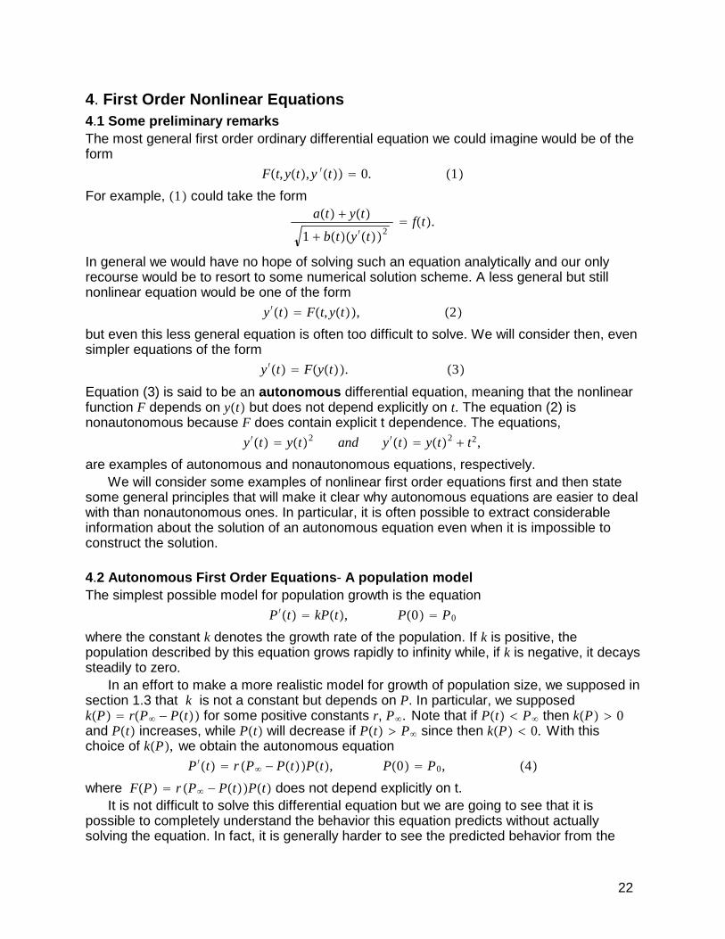
For any solution curve which starts at an initial value, P0, with 0 � P0 � P�, we canshow that P increases along this solution curve for all t � 0, and approaches the value P�asymptotically. The argument goes like this:At t � 0 we have P ��0� � r �P� � P0�P0 � 0, which means the curve starts out with Pincreasing. If there is a point on this solution curve where P�t� is not increasing, then therehas to be a time t0 � 0 where P ��t0� � 0 (i.e., in order for P�t� to be decreasing, it has to firststop increasing). Since this is a point on a solution curve where P ��t0� � 0 then (4) requiresthat either P�t0� � 0 or else P�t0� � P�. Clearly P�t0� � 0 is not possible since P started atP0 with 0 � P0 � P�, and P has been increasing since then. On the other hand,P ��t0� � 0 with 0 � P�t0� � P� is not possible either since this contradicts equation (4) whichasserts that P ��t0� � 0 only when P�t0� � 0 or P�t0� � P�. The only remaining possibility isthat a solution curve which originates at P0 with 0 � P0 � P�, must approach the horizontalasymptote P � P�, increasing steadily as t increases. In the same way, we can argue thatany solution curve that originates at P0 with P0 � P�, must approach the horizontalasymptote P � P�, from above, decreasing steadily as t increases. A plot showing threedifferent solution curves is shown below.

Figure 1 Solution Curves

The arrows on this plot indicate the slope of the P�t� versus t at each point in the plane. Wecan evaluate the slope, P ��t�, at each point �t, P�t�� by just evaluating F�P�t��.The collectionof arrows is called a "direction field" for this equation and any curve that is tangent to thedirection field at each point is called a solution curve or trajectory for the equation. The term"orbit" may also be used to refer to a solution curve.

4.3 Critical Points for Nonlinear EquationsConsider the autonomous nonlinear equation

P ��t� � F�P�t��.

We have defined a critical point for this equation to be any value P � P� such that

23

F�P�� � 0. Then we define an asymptotically stable critical point to be a value P � P�such that F�P�� � 0, with the additional condition that for any solution curve, P�t�,originating at a point P�0� near P�, it must follow that P�t� � P� as t � �. That is, P� isasymptotically stable if any trajectory that begins near P� must converge to P�. On the otherhand, a critical point P� for which the distance between P�t� and P� increasesas t � �, even for P�0� arbitrarily near P�, is said to be unstable. Equation (4) above hascritical points at P � 0 and P � P�. By examining the direction field in the figure above, wesee that the critical point at P � 0 is unstable, while the critical point at P � P� isasymptotically stable. That is, all the solution curves that start near P � 0 move away fromP � 0 and are attracted toward P � P�. Solution curves that begin either above or below thevalue P � P� tend toward P�.

It is possible for a critical point to be such that solution curves that begin on one side ofthe critical point are attracted back to the critical point while solution curves that begin onthe opposite side of the critical point are repelled and move away from the critical point. Acritical point with this kind of behavior is said to be "neutrally stable.

Now we state some general results about autonomous nonlinear equations. If weconsider the equation

y ��t� � F�y�t��, �5�

then

1. the critical points of (5) are the values y� for which F�y�� � 02. the critical point, y� is stable if F ��y�� � 03. the critical point, y� is unstable if F ��y�� � 04. distinct solution curves of (5) can never cross

Here point 1 is just the definition of critical point.Points 2 and 3 assert that a critical point, y�, for �5� can be classified as stable or

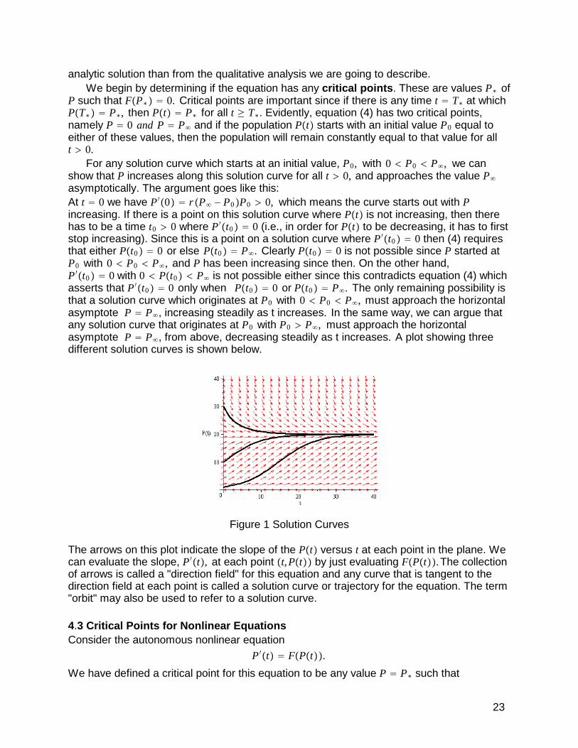
unstable by noting the sign of F ��y��. To see why the sign of F ��y� controls the stability ofthe critical point consider the example F�y� � �1 � y��y � 4�, which has critical points aty � 1, 4. The figure below shows the plot of F versus y. Consider first the critical point aty � 1. Note that for y slightly larger than y � 1, we have F � 0 which means y ��t� � 0 and yis increasing (i.e., moving away from y � 1 ). If y is slightly less than y � 1, then F � 0 soy ��t� � 0 there and y is decreasing. In either case, whether y is slightly less than or slightlylarger than y � 1, the value of y tends to move away from y � 1. At the critical point y � 4,the behavior is just the opposite. If y � 4, then F�y� � 0 and y increases and if y � 4 thenF�y� � 0 so y decreases. In either case, when y is close to 4 it will tend to move closer toy � 4.

24

1 2 3 4

-2

0

2

Figure 2 F(y) versus y

A more analytic argument is based on expanding F�y� about a critical point y�. That is,suppose F�y�� � 0 and write the first couple of terms of the Taylor series for F about y � y�

F�y� � F�y�� � F ��y���y � y�� � 12 F" �z��y � y��2.

If y is close to y� then 12 F" �z��y � y��2 is small relative to F ��y���y � y��, and since F�y�� � 0

we have

y ��t� � F ��y���y � y��

But y� is a constant so y ��t� � ddt �y � y�� and y � y� satisfies d

dt �y � y�� � F ��y���y � y��.Clearly if F ��y�� � 0, then y � y� will increase, while if F ��y�� � 0, then y � y� will decrease. Itfollows that the stability of the critical point y � y� is determined by the sign of F ��y��.

To see that point 4 must be true suppose that y � y1�t� and y � y2�t� are two differentsolutions of (5) whose graphs cross at some time t0. To say the graphs ”cross” at t � t0

means that y1�t0� � y2�t0�, and y1� �t0� � y2

� �t0�. ; i.e., the graphs go through the same pointbut have different slopes there. But if y1�t0� � y2�t0�, then F�y1�t0�� � F�y2�t0�� and thisimplies y1

� �t0� � y2� �t0�; i.e.,y1�t0� � y2�t0�

y1�t0� � y2�t0�

y1� �t0� � F�y1�t0�� � F�y2�t0�� � y2

� �t0�,

Clearly at a point where y1�t0� � y2�t0� the slopes cannot be different. This contradictionshows that solution curves are either identical or else they never cross. We say that thefamily of solution curves is coherent.

Using these observations about the behavior of autonomous first order equations it ispossible to sketch solution curves as in Figure 1. Such a sketch is called a "phase planeportrait" for the autonomous equation. The steps in making such a sketch are: i) find all thecritical points where F�y� � 0, ii) Classify the critical points as stable or unstable byevaluating F ��y��, iii) Plot a selection of solution curves starting on either side of eachcritical point.

ExercisesFor each of the following autonomous equations, find and classify the stability of all thecritical points and then sketch the phase plane portrait for each. In doing this, it will behelpful to plot F�y� versus y as in Figure 2. What will the plot of F�y� versus y look like whenthere is a neutrally stable fixed point?

1. y��t� � �y � 2��6 � y�2. y��t� � 9y � y3

25

3. y��t� � cos2y�t�

4. y��t� � 1 � y�t�2

5. y��t� � y�4 � y2�6. y��t� � y2�4 � y�2

5. Applications of First Order EquationsIn this section we are going to discuss a number of simple applications of first orderordinary differential equations.

5.1. Viscous FrictionConsider a small mass that has been dropped into a thin vertical tube of viscous fluid likeoil. The mass falls, due to the force of gravity, but falls more slowly than it would in a fluidlike water because the oil is thicker than water, (or, as we say, the oil is more viscous thanthe water). One of Newton’s laws asserts that the time rate of change of the momentum ofthe mass is equal to the sum of the external forces acting on the mass,

ddt

�mv�t�� � F

where m is the mass of the object and v�t� is the mass velocity as a function of time. Theforces acting on the mass are the force of gravity, Fg and the friction or viscous force of theoil, F f. Then

Fg � mg

and F f � �k v�t�,

where we have assumed that the friction force is proportional to the velocity (i.e., the fasterthe object moves, the more the oil retards it). The constant of proportionality, k, is assumedto be constant and then the negative sign appears in the definition of F f so that the forceacts in the direction opposite to the direction of the velocity. Then the differential equationbecomes

mv��t� � mg � kv�t�, v�0� � v0, �1. 1�

where v0 denotes the initial velocity of the mass. We can rewrite the equation in standardform as

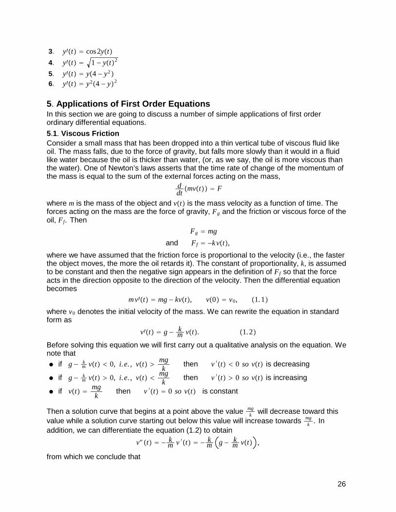
v��t� � g � km v�t�. �1. 2�

Before solving this equation we will first carry out a qualitative analysis on the equation. Wenote that� if g � k

m v�t� � 0, i. e. , v�t� �mgk

then v ��t� � 0 so v�t� is decreasing

� if g � km v�t� � 0, i. e. , v�t� �

mgk

then v ��t� � 0 so v�t� is increasing

� if v�t� �mgk

then v ��t� � 0 so v�t� is constant

Then a solution curve that begins at a point above the value mgk

will decrease toward thisvalue while a solution curve starting out below this value will increase towards mg

k. In

addition, we can differentiate the equation (1.2) to obtain

v" �t� � � km v ��t� � � k

m g � km v�t� ,

from which we conclude that

26

if v�t� �mgk

then v ���t� � 0

and if v�t� �mgk

then v ���t� � 0.

Then the solution curves above the value mgk

all have positive curvature and decreasetoward the limiting value v� �

mgk

. Those curves that begin below the limiting value havenegative curvature and increase toward v�. This constant could be interpreted as theterminal velocity of the projectile falling in the fluid..

The curve lying above the constant v� �mgk

is consistent with an object that is fired intothe oil with a large initial velocity in which case the projectile gradually slows down as itcontinues to fall only under the effect of gravity and the viscous drag of the oil. The curvelying below the constant represents the case where the object is introduced into the tubewith a small or zero initial velocity. In this case, the velocity increases toward the terminalvelocity mg

kdue to gravity and friction.

In order to now solve for v�t�, we note that equation (1.2) is equivalent to

� dvg � k

m v� � dt,

from which it follows that

� km ln g � k

m v � t � C0

or, ln g � km v � � mt

k� C1.

Then

g � km v � C2 e

� mtk ,

and

v�t� �mgk

� C3e� mt

k .

The initial condition is satisfied ifmgk

� C3 � v0 so, finally,

v�t� �mgk

� mgk

� v0 e� mt

k � v� � �v� � v0�e� mt

k ,

where we introduce the notation, v� �mgk

for the terminal velocity. This is an explicit

formula for the solution curves that were described above. Note that v�t� � x ��t� where x�t�denotes the position as a function of time. Then this position function can be obtained byintegrating the function v�t� with respect to t.

Exercises-1. Find x�t� if the initial position is x�0� � 0. .2. Discuss how you might solve for k if the parameters m, g are assumed known. Can youthink of an experiment for finding v�? If so, then k can be found from the knowledge of v�?3. Choose simple numerical values for m

k, v�, and v0 and plot v�t� versus t. Try both v� � v0

and v� � v0 and imagine what the curve is describing.

5.2. A Dissolving Pill

27

A spherical pill is dropped into a fluid where it begins to dissolve at a rate that is proportionalto the surface area exposed to the fluid. We can express this last statement inmathematical terms by writing

ddt

Volume � �K Surface Area �2. 1�

where K denotes a positive constant of proportionality and the minus sign indicates that thevolume decreases as long as the surface area is positive. For a sphere, we have

V � 43R�t�3 and SA � 4R�t�2

where R�t� denotes the radius of the sphere (which varies with t). Thenddt

Volume � ddt

43R�t�3 � 4R�t�2 R ��t�

and4R�t�2 R ��t� � �K 4R�t�2 ,

i.e., R ��t� � �K.

This is easily solved to obtain, R �t� � �Kt � C and then R �t� � R0 � Kt, where R0 denotesthe initial radius of the pill. Then it is easy to find the time for the pill to completely dissolve ifK is known. How might you go about finding K from an experiment?

5.3. Water Heating StrategySuppose a cylindrical water heater contains a heating element that electrically heats thewater in the tank . We have already seen this model, which we can write in the form

ddt

T�t� � k�Tf � T�t��,

where Tf denotes the temperature to which the water will be eventually heated if the heatingelement is left on constantly, and k is a positive constant that reflects the proportionalitybetween the time rate of change in the water temperature and the difference betweenTf and T�t�. Note that as long as T�t� is less than Tf, T��t� is positive so the temperature ofthe water increases. We must also account for the fact that there is heat lost to thesurroundings which we will assume is at a uniform temperature we will denote by S. Thisloss will produce a rate of change of temperature proportional to the difference between thetank temperature and the temperature of the surroundings. That is,

ddt

T�t� � K�S � T�t��

Here K denotes a positive constant so this equation asserts that as long as T�t� is greaterthan S, the temperature of the water will decrease. Now the water in the tank is beingsimultaneously heated by the heating element and cooled by loss of heat to thesurroundings so our equation that reflects this must have the form,

ddt

T�t� � K�S � T�t�� � k�Tf � T�t��

� KS � kTf � �k � K�T�t�.

Initially we have, T�0� � Tin, where Tin is the temperature at which the water enters thetank. It will be more convenient if we write this equation in the form

ddt

T�t� � �k � K��M � T�t�� �3. 1�

where

28

M �KS � kTf

k � K.

We know that we can solve this equation by writing

� dTM � T

� �k � K� � dt

which leads to

� ln�M � T�t�� � �k � K�t � C0

and

T�t� � M � C1e��k�K�t.

It follows from the initial condition that

T�t� � M � �Tin � M�e��k�K�t. �3. 2�

This solution predicts that the temperature will increase from Tin toward the limiting value Mat an exponential rate that is determined by the constants k and K. Note that M is atemperature between Tf and S and that M is close to Tf if K is very small, while M is closer toS if k is small compared to K. A small value of K corresponds to a tank that is well insulatedto there is little heat loss to the surroundings.

Now suppose that when the water temperature reaches some value Tmax � M, we turnoff the water heater. Note that we can use the solution for T�t� to determine the time ta atwhich the water temperature reaches Tmax; i.e. we solve

T�ta� � M � �Tin � M�e��k�K�ta � Tmax.

for ta. This gives

e��k�K�ta �Tmax � MTin � M

and

ta � �1k � K

ln Tmax � MTin � M

� 1k � K

ln M � Tin

M � Tmax.

Since the heater is turned off, the previous differential equation (3.1) is replaced by theequation

ddt

T�t� � K�S � T�t�� with T�ta� � Tmax �3. 3�

This describes how the water will gradually cool from a temperature of Tmax, as a result ofheat loss to the exterior. The solution of this new equation is found in the usual way to be,

T�t� � S � �Tmax � S�e�K� t�ta�

We can now suppose that when the temperature of the water reaches some selectedtemperature Tmin with S � Tmin � Tmax, we turn the heater back on again. The time tb whenthe temperature reaches Tmin is obtained by solving

T�tb� � S � �Tmax � S�e�K� tb�ta� � Tmin

to get

29

e�K� tb�ta� �Tmin � STmax � S

or tb � ta � 1K

ln Tmin � STmax � S

We now solve �3. 1� on the interval t � tb with the initial condition, T�tb� � Tmin. The watertemperature will increase toward M and we can then turn the heater off again when thetemperature reaches Tmax at some time tc � tb. In this way, the temperature is maintainedbetween limits Tmin and Tmax without the heater having to be on constantly.

5.4. Absorption of MedicationsWhen you take a pill to obtain medication, the pill first goes into your stomach and themedication passes into your GI tract. From there the medication is absorbed into yourbloodstream and circulated through your body before being eliminated from the blood by thekidneys and other organs. If we let x�t� denote the amount of medication in your GI tract attime t, then we can model the movement of the medication out of the GI tract with theequation

x ��t� � �k1x�t�, x�0� � A. �4. 1�

This is the assertion that after taking the pill, an amount A of medication is in the GI tractand it decreases at a rate proportional to the amount currently present in the GI tract. If theamount of medication in the bloodstream at time t is denoted by y�t�, then

y ��t� � k1x�t� � k2 y�t�, y�0� � 0, �4. 2�

expresses the fact that medication is coming into the bloodstream at exactly the rate it isleaving the GI tract and it is leaving the bloodstream at some rate expressed by theproportionality constant k2. Also, we are assuming that there is no medication in thebloodstream initially. Now this is two equations for the two unknown functions x�t� and y�t�,but the first equation can be solved independently and the solution substituted into theequation (4.2).

The solution of (4.1) is easily found to be

x�t� � A e�k1 t,

and then

y ��t� � k2 y�t� � k1x�t� � k1A e�k1 t.

We will find a particular solution for the y-equation by the method of undeterminedcoefficients. We guess that yp�t� � a e�k1 t and substituting this guess into the differentialequation, we find

yp��t� � k2 yp�t� � �k1a e�k1 t � k2a e�k1 t

� k1A e�k1 t.

This leads to

a �k1A

k2 � k1and yp�t� �

k1Ak2 � k1

e�k1 t.

Then

y�t� � C e�k2t �k1A

k2 � k1e�k1 t

and, using the initial condition to evaluate C, we get

30

y�t� �k1A

k2 � k1� e�k1 t � e�k2t�

Plotting x�t�and y�t� versus t for some representative values of the constants gives thefollowing figure

0 1 2 3 4 50.0

0.2

0.4

0.6

0.8

1.0

x

y

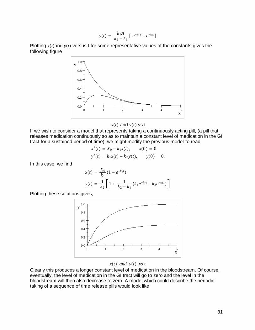
x�t� and y�t� vs tIf we wish to consider a model that represents taking a continuously acting pill, (a pill thatreleases medication continuously so as to maintain a constant level of medication in the GItract for a sustained period of time), we might modify the previous model to read

x ��t� � X0 � k1x�t�, x�0� � 0.

y ��t� � k1x�t� � k2 y�t�, y�0� � 0.

In this case, we find

x�t� �X0

k1�1 � e�k1t�

y�t� � 1k2

1 � 1k2 � k1

�k1e�k2t � k2e�k1t�

Plotting these solutions gives,

0 1 2 3 4 50.0

0.2

0.4

0.6

0.8

1.0

x

y

x�t� and y�t� vs tClearly this produces a longer constant level of medication in the bloodstream. Of course,eventually, the level of medication in the GI tract will go to zero and the level in thebloodstream will then also decrease to zero. A model which could describe the periodictaking of a sequence of time release pills would look like

31

x ��t� � X0�t� � k1x�t�, x�0� � 0,

y ��t� � k1x�t� � k2 y�t�, y�0� � 0,

where X0�t� denotes a piecewise constant function that alternates between a positive valueand zero. We will discuss an effective way to solve equations involving such terms when wediscuss the Laplace transform.

32