chapter one pet background - wellcome trust centre for ... · chapter one pet background ......

Andrew P. Holmes.Ph.D., 1994.

Chapter One

PET Background

An understanding of positron emission tomography and the various imageprocessing techniques involved in the preparation of images of blood flow is essential totheir analysis.

In this chapter we outline the fundamentals of positron emission tomography toprovide the background to the data we consider in subsequent chapters. We review thestatistical aspects in detail. The overall aim is to provide a general background to PET, ata level of exposition suitable for the newcomer.

Those familiar with the concepts and terminology of functional mapping may wishto skip most of this chapter, perhaps reading only the description of the “V5” dataset (§1.7.) before proceeding to chapter 2. Similarly, the reader with little time mayprefer to accept that images whose intensity is indicative of regional neuronal activity canbe obtained with PET, note the description of the “V5” study, and also proceed tochapter 2.

5

6 Chapter One: PET Background

1.1. Additional Reading

Overviews of PET

There exist various reviews of PET and Neuroimaging that may be of interest.Ter-Pogossian et al. (1980) review PET in its early days. They describe the mechanics ofPET: the preparation of isotopes, physics of electron annihilation and event detection, andreconstruction. The description of filtered back-projection is especially clear. Ofparticular interest is their discussion of tracer kinetics, and the problems of obtainingquantitative images from tracer density. They look forward to the “future” of PET,concentrating on the study of the heart, and their discussion provides an introduction toheart-PET.

The paper by Raichle (1983b) briefly covers the main ingredients of PET. Thispaper also contains an excellent review of tracer kinetics, and the assumptions inherent inobtaining quantitative measurements of metabolic processes, and ends with a sectiondetailing possible clinical applications of PET.

Brownell et al. (1982) gives an even briefer review of PET. Despite the age of thispaper, it does provide a useful overview of nuclear Magnetic Resonance Imaging (MRI),and contains extensive references for the theory of PET and MRI.

State of the art“Positron Emission Tomography and Autoradiography”, edited by Phelps et al.

(1986) is a collection of chapters written by experts in the various disciplines associatedwith positron emission tomography. This book represented the state of the art in the mid-eighties, and still constitutes the single most thorough exposition of PET methodology.

For more recent information, the published proceedings of recent conferences areuseful. The “Brain PET” bi-annual conference was first held during June 1993 in Akita,Japan, with proceedings “Quantification of Brain Function: Tracer Kinetics and ImageAnalysis in Brain PET” edited by Uemura et al. (1993).

JournalsThe main journals for the publication of PET methodology are the Journal of

Cerebral Blood Flow and Metabolism and the Journal of Computer AssistedTomography. Recently Human Brain Mapping has emerged, a journal dedicated tofunctional neuroimaging to which many researchers are now sending their papers,particularly those working in functional MRI (fMRI).

Data Acquisition 7

1.2. Data Acquisition

1.2.1. The TomographThe positron tomograph essentially consists of a cylinder of bismuth germanate

(Bi4Ge3O12) detectors arranged in rings. A recent dedicated brain scanner (ECAT 953B,Siemens/CTI, Knoxville, Tennesee, described by Spinks et al., 1991) has 16 rings, eachof 384 detectors of size 5.6×56.45×30mm3. The detectors are grouped into blocks of8×8, mounted on a set of four photomultiplier tubes. The detector hit in an 8×8 block isobtained by combining the readings from the four photomultipliers, using Anger logic.The ring diameter is 76cm, with an axial length of 10.8cm. The patient port size is 35cm.

Figure 1Schematic of the arrangement of detectors in a PET tomograph

1.2.2. Data acquisition

Subject preparation, isotope decay, electron annihilationThe subject is positioned in the tomograph, using external landmarks (eyes, ears)

for rough alignment. A chemical labelled with a positron emitting isotope is introducedinto the subject, either intravenously or by inhalation of a gas.

The radioisotope decays, each decay event resulting in the emission of a positron.The positron loses kinetic energy as it travels through the surrounding tissue. After about1–6mm the positron is highly susceptible to interaction with an electron. This results inthe annihilation of both particles, their mass being conserved as energy by the emission oftwo photons of gamma radiation, each of energy 511keV. Conservation of momentumdictates that the two photons will be emitted in almost opposite directions (fig.2), thecolliding positron having little momentum. The axis of the pair of emitted gammaphotons is completely randomly oriented.


β+

e-

e-

e-

e-

e-

e-e-

e-

e-

e-

e-

e-

e-

e- e-

e+

e+

5 mm

positron emitter

positron

electron

positron path

511 keV gamma ray photon

approx 5o

β+

Figure 2Positron emission, electron annihilation and gamma ray emission

Detection of annihilation events, VORsThese two photons of gamma radiation then travel through the tissue and air. If the

two photons are detected by the tomograph, then two crystals will be hit atapproximately the same time. These two crystals then define a volume of response (VOR)in which the electron annihilation must have taken place (fig.3). The tomographcomputer counts the number of times the two detectors defining each VOR are hit(almost) simultaneously during the scanning period.

a

b

electron annihilation

511keV gamma ray photon

volume of response defined bydetector pair a-b

subject

ring of detectors

Figure 3Schematic of detection in a PET tomograph

1.2.3. SinogramsThese VOR counts are stored as sinograms. A sinogram is an image of the VOR

counts for a particular ring of detectors (direct plane sinograms), or for a pair of rings(cross plane sinograms). For a 16 ring tomograph, 256 sinograms are acquired, 16 directplane sinograms and 16×15 cross plane sinograms.

A direct plane sinogram is constructed as follows: Let the number of parallel VORspossible be p; and the number of detectors in the ring 2n. Then from a given starting

Data Acquisition 9

point in the ring, consider the p parallel VORs defined by that detector, and the p-1detectors round from it, with the p opposing detectors (fig.4). The counts for these pVOR constitute the pixel values for the first row of the sinogram. Subsequent rows of thesinogram are obtained by considering the p parallel VORs defined by the p detectors onealong from the previous set. There are n sets of p parallel VORs for a single ring, givingan n×p sinogram. Cross ring sinograms are similarly formed: Each row consists of thecounts for the p parallel VOR defined by p detectors in one ring and the opposingdetectors in the other ring. There are 2n sets of p parallel VOR, giving a 2n×p sinogram,which is split up into two of dimension n×p.

one line of sinogram

p volumes of response

Figure 4Construction of one line of a sinogram

A direct plane sinogram for a non-central point source will be a sine wave (fig.5).Hence the name sinogram. For the ECAT 953B n is 192 and p is 160.

Figure 5Sinogram for a non-central point source


Figure 6Direct plane sinogram from a scan of the authors brain. Data frame energywindow sinogram 64 of run 12 on subject n278. Acquired on an ECAT-953B

dedicated brain scanner, February 1992, during a visit to the MedicalResearch Council Cyclotron Unit at the Hammersmith Hospital, London.

1.2.4. Additional dataIn addition to the VOR counts for the scan of the subject, a number of additional

measurements have to be taken. These are to allow corrections for detector efficiency,attenuation, background radiation, scatter and randoms. We briefly describe each in turn,to give some insight into some of the more problematic physical aspects of PET scanning.A comprehensive discussion of quantification for positron emission tomography can befound in Hoffman and Phelps (1986).

Normalisation–Blank scanIt is impossible to manufacture the detector crystals and associated electronics such

that all the detectors have the same sensitivity. Discrepancies in detector sensitivitiesshow up on sinograms as light sinusoidal “streaks” (fig.6). To correct for the relativedifferences in sensitivity a blank scan is acquired at the beginning of each day.

During the blank scan radioactivity is provided by three positron emitting rodsaligned parallel to the axis of the tomograph, which are rotated about the axis of thetomograph to give the appearance of a uniform source to all the detectors. Acquisition iscontinued over a long period, so that the number of recorded events for each VOR is

Data Acquisition 11

great. The relative sensitivities of the detector pairs for each VOR, can then be accuratelyestimated by the differences in detection rates.

These relative sensitivities can be built into the statistical model for PET, or can beused to correct observed VOR counts by a simple scaling. The latter is usually used inpractice.

Transmission ScanAlthough the photons of gamma radiation emitted following the annihilation of

positron and electron have a relatively high energy of 511keV, some are absorbed by thetissue through which the photons have to pass in order to reach the detector. Theprobability of attenuation is related to the density to gamma rays of the tissue along theline of flight. To estimate this density, a transmission scan is taken during the scanningsession, usually at the beginning or the end.

The subject is positioned in the scanner as usual, but no tracer is introduced. Therotating rod sources provide a uniform source of gamma rays. Data is acquired for aboutthree minutes, such that the detection rates for each VOR can again be regarded asaccurately estimated by the observed detection rates. The ratio of this rate to the blankscan rate for each VOR is then an estimate of the probability of non-absorption along theVOR. These attenuation probabilities can then be built into the model for PET

reconstruction, or can be used to correct the observed VOR counts by a simple scaling.Again the latter is usually used in practice.2

Background radiationFor a simple scan, two sets of sinograms are acquired. The scan is split into two

time frames, the background frame and the data frame. The radiotracer is introduced atthe beginning of the data frame. The sinograms for the background frame indicate thestructure of background radiation and any residual activity from a previous scan.

The background frame may be used to estimate and remove background andresidual activity. However, due to the low activity, the number of detected events is low,and estimates are highly variable. This is evidenced in the noisy appearance ofreconstructed background frame images. Any linear correction of a data frame thereforeadds this noise to the image.

2It is possible to reconstruct the three-dimensional linear attenuation function. This is known astransmission tomography and is considered again in the filtered back-projection subsection of thereconstruction section (§1.4.3.1., p.22).


ScatterScatter occurs when one (or both) of the emitted gamma photons are deflected

during their passage to the detectors, possibly leading to detection in a VOR that does notcontain the point of annihilation (fig.7).


511keV gamma ray photon

volume of response incorectlyidentified for annihilation

subject

ring of detectors

gamma photon deflected here

Figure 7Scatter

To counter the effects of scatter, the energies of the detected photons can be used,as a photon will lose some of its 511keV of energy when it is scattered. If only photonswith energies lying in a predefined energy window containing 511keV are considered,and a VOR count only recorded for almost simultaneous detection of two photons withenergies lying in this window, then some scatter should be eliminated.

However, there will still be some scattered photons with a high enough energy tobe in the energy window, as illustrated in fig.8. To enable a correction for this, two setsof VOR counts are collected. One set for coincident detection of photons with energies inthe energy window, and one set for coincident detection of photons one or both of whichhave energies in the lower window.

freq

uenc

y

photopeak

photon energy

511 keV380 keV 850 keV

lower energy window energy window

all detected photons

scattered photons

direct photons

Figure 8Energy distribution of detected gamma photons

Data Acquisition 13

The simplest correction proceeds by subtracting a fraction of the lower energywindow sinograms from the upper energy window sinograms. (That is, a fraction of theVOR counts for the lower window are subtracted from the from the corresponding VOR

counts for the upper energy window, for each VOR.) The fraction used is ideally thefraction of the scattered photon energy distribution appearing in the upper energywindow, the scatter fraction. This can be estimated using phantom studies, in whichsources of known radioactivity are scanned once when surrounded by water, and once ina vacuum, when there will be no scatter. The assumption implicit in such a correction isthat the structure of the events in the lower energy window (predominantly scatteredevents) is shared by the scattered events of the upper energy window. Scatter is anartefact of the radiotracer density and the tissue density (to gamma rays) of the subject,so the assumption is not unfounded.

The low count rates for the lower energy window results in estimates of scatterthat are very variable, so scatter correction adds noise. More sophisticated methods forscatter correction are the subject of current research.

Multiple incidencesA multiple incidence occurs when three or more detectors are hit (almost)

simultaneously. In this situation, a VOR can not be identified, and the events are ignored.

RandomsRandoms are multiple incidences, where two (nearly) simultaneous annihilations

have exactly one photon detected. The VOR defined by the two detectors has its countfalsely incremented.


1.3. 2D & 3D PET, SPECT

1.3.1. 2D & 3D PET

Until recently, algorithms for reconstructing three dimensional images from allpossible VOR counts were not in common use. Reconstruction was only possible in twodimensions, reconstructing a slice of the subject from each direct plane sinogram. Theslices were then stacked to obtain a three dimensional image. Only VORs correspondingto detector pairs in the same ring could be considered. Some limited cross ring VORswere allowed to enable planes between the rings to be considered, with induced planesinograms formed by averaging counts between adjacent rings. This type of PET is knownas 2D PET. For a 16 ring tomograph there would be only 31 sinograms, 16 direct planesinograms, and 15 induced plane sinograms.

As 2D PET only needs VOR counts for direct plane and limited cross ring VOR

counts, older scanners have fixed tungsten collimating septa around the detectors,reducing the view of each detector to detectors in the same and adjacent rings. This hasthe effect of reducing the detection of randoms, scatter, multiple incidences andbackground radiation. Scanners produced in the early nineties have removable septa,enabling data acquisition for 2D or 3D PET (fig.9), and new scanners operate solely in 3Dmode.

septa extended

septa retracted

Cross sections througheight rings of detectors

tungsten septa

Figure 9Septa

Sensitivity of 3D PET

In 2D mode, less than 1% of the annihilation photon pairs are detected(Cherry et al., 1991, p655). Removal of the septa greatly enhances the sensitivity of thetomograph: The probability of both gamma photons from an annihilation event hittingdetector blocks is on average about six times greater (Spinks et al., 1991), with largerincreases for annihilations occurring near the centre of the scanner.

For a subject with radioactivity suitable for a 2D study, the rate of photons hittingthe detectors in 3D mode is so high that many are not detected because of the detector

2D & 3D PET, SPECT 15

dead time.3 This saturation of the tomograph is avoided by using lower doses ofradioactivity, typically a quarter of the dose administered in 2D (Cherry et al., 1991).4

Removal of the septa and acquisition of all lines of response makes the scannermore likely to detect scattered photons, multiple incidences, randoms and backgroundradiation. So, raw count rates can not be used to compare the sensitivity of 2D and 3Dmodes of PET acquisition. Noise Equivalent Counts (NEC), due to Strother et al. (1990),measures count rate relative to image signal-to-noise ratios by accounting for scatter andrandoms. Using this measure, Bailey et al. (1991) found that for activity concentrationssuitable for a 3D acquisition (< 1µCi/cc, corresponding to an injected dose ofapproximately 28mCi), the NEC was around five times that for 2D mode. Furthermore,this NEC was slightly better than that of a 2D acquisition with four times the activity.Cherry et al. (1993) present similar findings, using (grey matter) standard deviation insingle difference images rather than NEC as the measure of scanner sensitivity.

Summary: 3D better than 2DThus 3D acquisition provides images of comparable quality to 2D mode, but

requires the administration of less radiation to the subject per scan. This allows morescans to be taken on an individual for the same total injected dose, giving more data, andhence improving the power of statistical procedures to analyse data sets of images fromsuch experiments. This has been evaluated in blood flow studies of the human brain byBailey et al. (1993) in terms of NEC, and by Cherry et al. (1993) in terms of estimatedstandard deviation in mean difference images5 from phantom6 data. Both these papersreport a two-fold increase in sensitivity of the 3D method using four times as many scansas the 2D method, for the same administered activity. Further fractionalisation of thedose gives further improvements, but leads to an unacceptable number of scans.

1.3.2. SPECT

There are radio-chemicals available that emit gamma rays directly on decay. Asingle photon is emitted, so a special tomograph is required, commonly referred to as agamma camera. The radio-chemicals in question are less radioactive than positronemitters, do not require a high power cyclotron to produce them, and can be handledeasily. The isotopes involved have long half lives, so tracers can be made remotely. Thismakes Single Photon Emission Computed Tomography (SPECT) a financially viableclinical tool, and most large hospitals possess a SPECT tomograph.

3When gamma photon hits the detector crystal, a scintillation event takes place causing the block toflash. The flash is detected by the photomultipliers which generate an electric signal. A scintillationevent takes a small time to take place, during which incident gamma photons go undetected. This periodis called the dead time4About 50–80 mCi H215O is injected into subjects to obtain a satisfactory 2D acquisition.5Mean difference images are introduced in §2.3.1.1. where the simple paired t-test approach for multiplesubject activation studies is discussed.6A phantom, in radiography, is a shaped container containing a known concentration of activity. Themost famous is the Hoffman brain phantom (Hoffman et al., 1990).


The SPECT tomographSince only one gamma photon is emitted by the decaying isotope, the detectors of

a SPECT tomograph need to be shielded by lead collimators so that each has a narrowfield of view, enabling the identification of a VOR for a detected emission (fig.10).


gamma ray photon

subject

gamma camera head

lead collimators

observed decay event

decay event not seen (attenuated)

observed background radiation

decay event not seen (collimation)

decay event not seen (misses camera)

VORs

Figure 10Schematic of a simple SPECT gamma camera. The camera head is positionedat various places around the subject to enable data to be collected for manyVOR.

Resolution of SPECT scansThe resolution of SPECT imaging is much lower than that of PET for a number of

reasons. The low energy gamma rays (140 KeV for technetium-99m, 99mTc) are veryprone to attenuation, resulting in decay events not being observed. The restricted field ofview of the detectors also reduces the probability of observing the gamma radiationemitted by a decaying isotope. As a result of this, and the low activity of SPECT tracers, aSPECT scan is usually acquired over quite a long period, typically in the region of twentyminutes. Even then, the number of observed decay events is still quite poor combinedwith PET, being a couple of orders of magnitude smaller. These low counts lead to highlyvariable estimates of tracer concentration, apparent in reconstructed images as noise.Background radiation is of comparable energy to the gamma rays of SPECT, and itsdetection adds to the noise in SPECT images. To obtain VOR counts of sufficient size forreasonable reconstruction, gamma cameras use larger detectors than a positrontomograph, resulting in fewer VORs and hence lower reconstructed resolution. For acomprehensive overview of SPECT, see English and Brown (1986).

Advantages of PET over SPECT

The poor quality, long scan times, and long half lives of the tracers (precludingmultiple scans on the same individual) in SPECT make the expense of PET justifiable, atleast for research. In addition the array of gamma emitting tracers is somewhat limited,and many biochemicals can only be labelled with positron emitters. PET has widerbiological scope, and is a more powerful research tool.

Reconstruction 17

1.4. Reconstruction

The raw data acquired by the tomograph are the VOR counts. These are thenumbers of annihilations on a particular VOR resulting in detected gamma radiation alongthat VOR. From this data it is desired to estimate the regional decay rates, or regionalactivity (rA), as this indicates the distribution of the tracer.

1.4.1. A statistical model for PET

Let n*=(n*1,…,n*

r ,…,n*R) be the vector of counts for the R VORs. These are clearly

realisations of random variables, the form of which we now derive. The model followsthat of Vardi et al. (1985).

Average emission intensityThe radioactive decay of the positron emitting isotopes in the subject forms an

inhomogeneous Poisson process in both space and time. Let the intensity of this processbe λ(x,t); for position x∈Ξ and time t, measured from the start of the scan, which wetake to be of length T. Here Ξ is the subset of Euclidean 3-space ℜ3 corresponding tothe image space of the tomograph, for suitable Cartesian axes.

If we assume a constant tracer density over the duration of the scan, then this canbe expressed as λ(x,t) = λ(x,0) exp(-βt) by the law of radioactive decay, where λ(x,0) isthe emission rate at the start of the scan. β is related to the half-life of the tracer, t1/2, byβ=ln(2)/t1/2, and is hence known.

Over the scan period, t∈[0,T], the emission intensity at x∈Ξ is:

( ) ( ) ( )

( )( )( )

λ λ β

λ

βλ

β

x x

x

x

, dt , exp d

,

t t t

e

T T

T

0 0

0

0 1

∫ ∫= −

=−

=

−

say

(1)

so it suffices to estimate λ(x), the average emission intensity.

Model for average emission intensityLet c(x,r) be the probability that an emission from x results in an electron

annihilation detected in VOR r. Then, the emissions from point x detected in VOR r, forma thinned Poisson process with thinning probability c(x,r), independently for all x∈Ξ andr =1,…,R. Thus the number of detected emissions for the VORs, n*r , are independentPoisson random variables with means

[ ] ( ) ( )E c , d* *n rr r= =∈∫λ λ x x x

x Ξ

(2)

and we want to estimate λ(x) given n*r .


Discretisation of the problemTo simplify the mathematics, and to avoid the estimation of a continuous function,

it is usual to consider Ξ divided up into K voxels7 (volume elements), usually cuboid inshape. Within each voxel λ(x) is assumed to be constant.

Let {Vk} Kk = 1 be a partition of Ξ into K voxels. That is Vk⊂ Ξ, k = 1,…,K;

Vk ∩ Vk' = φ for k≠k'; and Uk=1

KVk = Ξ. We shall refer to voxels directly by their index,

referring to the voxel with index k (the volume element Vk), simply as “voxel k”.

Discrete model for average emission intensityThe number of emissions within voxel k over the period of the scan is a Poisson

random variable, with mean

λk = ( ) ( )λ λx x x x, d d dt tT

V Vk k0∫∫ ∫=

≈ |Vk| λ(x)

for some x∈Vk, if λ(x) is fairly constant within Vk, where |Vk| is the volume of voxel k.

Thus λk / Vk is a step function approximating λ(x), and we proceed to estimate

λλ = (λ1,…,λK). Substituting this approximation into eqn.2 gives:

[ ] ( )Ε n k rr r kk

K* * p ,= =

=∑λ λ

1

r = 1,…,R (3)

where p( , ) c( , )dk rV

rk Vk

= ∫1

x x

Eqn.3 defines a Poisson regression equation expressing the observed VOR countsn*r in terms of λλ, which it is desired to estimate, subject to the positivity constraintsλk ≥ 0, k = 1,…,K. The average emission intensity for voxel k, λk, is referred to simply asthe regional activity (rA) at voxel k. Since λk is expressed in counts per unit volume,reconstructed images are known as counts images.

Computation of detection probabilitiesThe p(k,r) are the probabilities that an emission occurring in voxel k is detected in

VOR r, the detection probabilities. Ignoring positron flight, attenuation, scatter, detectorinefficiencies and assuming that the two gamma photons are emitted in oppositedirections, this probability is (up to a normalising constant) the angle of view of VOR rinto voxel k, and can be computed from a knowledge of the scanner geometry.

Positron flight, attenuation, detector inefficiencies and the angle of gamma photonscan all be built in to these probabilities, see Vardi et al. (1985) and Shepp et al. (1982)for further details. These refinements make computation of the p(k,r) more lengthy, toolengthy for computation on the fly to be efficient, and the probabilities must be computedand stored, requiring considerable storage space.

7Voxel, is the 3D analogue of a pixel, which is short for “picture element”.

Reconstruction 19

This computation is made notably simpler (especially in 2D PET imaging) by theconsideration of an annular array of voxels, with the number of voxels per annulus somemultiple of the number of detector elements per ring. With this arrangement, proposed byKearfott (1985), Each detector element would view exactly the same arrangement ofvoxels and opposing detector elements as any other detector element (in that ring, for the3D case). This greatly reduces the number of distinct p(k,r). Kaufman (1987) discussesan implementation of such a method. If an attenuation correction more complicated thanthat for a rotationally symmetric attenuating medium (with axis that of the tomograph) isbeing considered, then there is no symmetry, and the advantages of an annularvoxellation are lost, a point noted by Green (1985).

1.4.2. Maximum Likelihood ReconstructionVardi et al. (1985) discuss the maximum likelihood estimation of λλ. The likelihood

of the observed data is:

( ) ( ) ( ) ( ) ( )

( )L P

!*

*

*

**

λλ λλ= = −

=∏n e

r

n rr

n r

r

Rλ λ

1

giving log-likelihood

( ) ( )( ) ( ) ( )( )

( ) ( ) ( )

l n n

k r n k r n

r r r rr

R

kk

K

r kk

K

rr

R

λλ λλ= = − + −

= − +

−

=

= ==

∑

∑ ∑∑

ln L ln ln !

p ' , ln p ' , ln !

* * * *

'

*

'

*

λ λ

λ λ

1

1 11

with first partial derivative with respect to λk as

( ) ( ) ( )

( )

∂∂λ λ λ

λ

lk

n k r

k rk

k kr

kk

Kr

Rλλ = − • +

=

= ∑∑p ,

p ,

p ' ,

*

'' 1

1

(4)

where p(k,•)=∑r=1R p( )k,r is the probability that an emission in voxel k is detected.

Vardi et al. (1985) show that the matrix of second partial derivatives of l(λλ) isnegative semi-definite, and hence that l(λλ) is concave. Thus the single local maximum (ifit exists) is a global maximum over λλ∈ℜ3, and can be found by setting the first partialderivative to zero.

Bearing in mind the positivity constraint on λλ (λλ ∈ {ℜ+×…×ℜ+}), sufficient

conditions for λλ̂ to be the maximum likelihood estimator of λλ are the Kuhn Tuckerconditions:

∂l(λλ)λk λλ̂

= 0 and∂l(λλ)∂λk λλ̂

≤ 0 if λ̂k = 0


There are many possible schemes for solving to obtain λλ̂. A particularly simpleiterative scheme suggested by the form of the partial derivatives (eqn.4) is:

( )( )

( )( )

( ) ( )λ λ

λki k

ir

ki

k

Kr

R

k

n k r

k r

+

=

==

• ∑∑1

1

1p ,

p ,

p ' ,

*

''

(5)

giving a sequence λλ(1),…,λλ(i),… converging to the maximum likelihood estimate λλ̂. This can be thought of as a preconditioned steepest ascent method, having propertiessimilar to steepest ascent in many situations and considerably improving on it in others(Kaufman, 1987). This iterative scheme is an instance of the EM algorithm, as we shallnow illustrate.

EM reconstructionHere we have a classic example for the application of the EM algorithm of

Dempster et al. (1977). The ideal data would be the number, nk, of detected emissions ineach voxel (k =1,…,K). The available data are the VOR counts. Both are marginal sumsof the quantities nkr, the number of emissions in voxel k detected in VOR r(k =1,…,K; r=1,…,R). The VOR counts, n*

r , can be viewed as incomplete data, with thenkr as complete data.

With this in mind, Vardi et al. (1985) re-formulate the problem as follows:Emissions in voxel k subsequently detected in VOR r form a Poisson process with meanλkr =

def λk p(k,r), since it is a thinning of the emission process, independently for allvoxels k and VOR r. Thus the number of detected emissions in voxel k, nk, is a Poissonrandom variable with mean

E[nk] = ∑r=1R λkr = λk p(k,•) (6)

The estimation, or E-step, is to estimate nk as n̂k, given λλ(i) and the data n*r.

( )

( )

( )

( )

( )

( )

( )

( ) ( )( ) ( )

( ) ( )

n n

n

n

n n n

n X a

X X x x

n k r

k r

k ki

kri

rR

kri

rR

kri

rrR

r

r kri

k ri

kK

r

R i i

i ia

a

ki r

ki

kK

r

R

i

i

^ *

*

*

* *

*

''* *

*

''

E ,

E ,

E ,

E ,

~ Po

~ Bin ,

p ,

p ,

=

=

=

=

=∑ =

=

=

=

=

== ∑

==

∑

∑

∑

∑∑

∑∑

λλ

λλ

λλ

λλ

n

n

n

1

1

1

11

11

by independence of ' s

since if , λ

λ

λλ

(7)

Reconstruction 21

The maximisation step, or M-step, is to obtain λλ(i+1), the maximum likelihoodestimate of λλ, given the current estimated detected emissions from voxel k. Since nk is a

Poisson random variable with mean λk p(k,•), (eqn.6), λ(i)k = n̂k / p(k,•).

Combining the E and M steps gives the iterative scheme of eqn.5. It then followsfrom Theorem 1 of Dempster et al. (1977) that l(λλ(i)) < l(λλ(i+1)). Since l(λλ) is convex,convergence to the maximum likelihood estimate (on this voxellation, see below) isguaranteed. See Vardi et al. (1985) for a proof and discussion.

There are two interesting properties of this EM solution. Firstly, the total counts arepreserved:

∑k=1K λnew

k p( )k,• = ∑r=1R n*r

Secondly, if λoldk > 0 then λnew

k > 0 also, for all voxels k=1,…,K. That is, the positivity

condition is satisfied for positive starting values.

Comments on the maximum likelihood approachShepp & Vardi (1982) tested their EM approach for 2D PET against a filtered back-

projection method, and (in Vardi et al., 1985) against a least squares method, usingsimulated data. Shepp et al. (1984) test the EM approach with real phantom data,comparing the reconstructed images with those from filtered back-projection. In all thepapers the EM reconstruction was preferred on visual grounds for lack of reconstructionartefacts and for aesthetic appeal. Mintun et al. (1985) also reported an improvement inresolution in EM reconstructions over the standard filtered back-projection for a lowresolution 2D camera.

Lange & Carson (1984) also developed EM algorithms for emission andtransmission tomography, aiming their exposition at a mathematically literate audiencefamiliar with tomography.

Kaufman (1987) discusses the practicalities of implementing the approach.Consideration of positron flight, detector inefficiencies and the non-linearity of the twogamma photons (but not attenuation or scatter) in the computation of the detectionprobabilities p(k,r) improved 2D reconstructions very little. Indeed, vast simplificationswere made in the computation of these probabilities, without substantial degradation ofthe reconstruction.

The maximum likelihood solution is not necessarily unique, indeed it cannot beunique if the number of VORs (R) is less than the number of voxels (K). The algorithmconverges to one of the reconstructions maximising the likelihood, depending on thechoice of initial values. Thus for cubic voxels, a unique solution for the EM algorithmimposes a lower bound on the voxels size, this size dependent on the geometry of thescanner. For voxel sizes smaller than this critical size the estimated value is not unique,but it is argued (Shepp & Vanderbei ([23] in Green, 1990)) that for typical data sets thepositivity constraint renders the maximum essentially unique.

Convergence to the maximum likelihood function estimate λλ̂ (for this voxellationof Ξ) is guaranteed, but may take a long time. Knowing when to stop the iterations is asource of indeterminacy. Stop too soon and a vague image is recovered. After manyiterations the estimate λλ(i) becomes very noisy, a common feature of maximum likelihoodestimates for images. Silverman et al. (1990) illustrate this vividly. Vardi et al. (1985)suggest using a small degree of smoothing on the maximum likelihood estimate, or aconstant starting estimate λλ(0) and fixed (small) number of iterations (for example 64).This latter scheme, starting with a level playing field and iterating until an “appealing”


estimate is found, is commonly called “Maximum Likelihood” reconstruction by PET

practitioners, though the estimates obtained are far from the actual MLE.Silverman et al. (1990) considered the above points and applied their smoothed EM

algorithm, the EMS algorithm, which introduces an S step after each EM iteration,spatially smoothing the current estimate λλ(i). This gives aesthetically pleasingreconstructed images which are quite smooth and free from the obvious reconstructionartefacts that plague filtered back-projection. The smoothing step reduces the spectralradius of the EM iteration, and thus accelerates convergence. Experience suggests thatconvergence is to a unique solution, although only approximate theory exists to back upthis assertion. However, there is little justification for the smoothing in this form, andthese images were criticised by Ford (1990) for being too smooth, as interest is in morethan the “picture” of the annihilation events.

Although the EM algorithm has been successfully applied to reconstruction it isn’tused in practice. This is partly because of the noisiness and indeterminate stoppingcriteria for the iterations, but mainly because computationally it is much more intensivethan filtered back-projection, especially for 3D reconstruction. Current interest instatistical reconstruction is concentrated on the use of prior information in an empiricalBayesian context, a review of which is beyond the scope of this chapter.

1.4.3. Filtered Back-projectionFiltered Back-projection (FBP) is the reconstruction method routinely used in most

circumstances. Essentially the counts are “projected” back across the image space,interfering to give an image of estimated counts per voxel. The technique was developedto reconstruct images from projections in fields as diverse as gravitation theory, radioastronomy and electron microscopy. More recently the technique has been used intransmission tomography, particularly X-ray computed tomography (X-ray CT).8 Shepp &Kruskal (1978) review the history of CT, and look at the various methods ofreconstruction from a mathematical perspective. Emission tomography developed fromtransmission tomography, and the existing reconstruction methods were adapted for thenew modality. Thus to review FBP we first look at transmission tomography and how itrelates to the PET problem.

1.4.3.1. Transmission tomography

In transmission tomography, parallel beams of monochromatic9 X-rays of constantintensity10 Iin (in counts per second) are directed through a thin slice of the subject, andthe number of X-ray photons transmitted through the subject from each beam ismeasured. This is done for a number of orientations, resulting in a data structure similarto that of PET (Fig.11). The quantity of interest here is the tissue density to X-rays, thelinear attenuation function µ(x).

8X-ray CT is commonly referred to a CAT, an acronym for Computerised Axial Tomography, the word“axial” emphasising that the X-rays are administered perpendicular to the axis of conventional X-rayimaging.9The source is assumed to be monochromatic, that is only X-ray photons of a given energy are emitted.Alternatively, one can assume that the physical attenuation is independent of the energies of the X-rayphotons.10That is the source has a half-life so long that the rate of decay can be considered constant for the timeperiods in question.

Reconstruction 23


gamma ray photon

subject

detector head

lead collimators

absorbed radiation

transmitted radiation

VORs

gamma radiation source

Figure 11Schematic of transmission tomography

For a line segment δ ⊂ ℜ3 through a medium with linear attenuation function µ(x),the total attenuation along the line is µδ, given by the Radon transform:

µδ = ⌡⌠δ

µ(x)dx (8)

Estimation of µδ in transmission tomography

For any X-ray photon travelling along δ the probability of non-absorption, isproportional to exp(-µδ), so the process of X-ray photons arriving at the detector is a

thinning of the emission process. The thinning probability is estimated by ninδ ÷ nout

δ ,

where ninδ and nout

δ are the numbers of photons emitted by the source, and the number of

those transmitted, respectively. Clearly it is impossible to count both. However, since

intense X-rays are used, ninδ ÷ T ≈ Iin , where T is the length of the acquisition for line δ.

This gives Iin × T ÷ noutδ as a good estimate of the thinning probability, and hence of µδ.

1.4.3.2. Approximation of emission tomography problem to fittransmission tomography framework

Emission tomography can be thought of in this framework, by assuming that theprobability of a positron emission from point x∈X being detected by the pair of detectorsdefining VOR r, c(x, r), is constant for all points x within VOR r, and zero for all otherpoints. Then, eqn.2 simplifies to

[ ] ( ) ( )E c , d* *n rr r

Vr

= = • ∫λ λ x x (9)

Here Vr⊂ X is the set of points in VOR r, and c(•, r) is the probability an emissionoccurring inside VOR r is detected by the detectors defining that VOR.


Eqn.9 is now in the same form as for transmission tomography. The observed datan* are taken as estimates of the VOR intensities λλ* , and an estimate of λ(x) is soughtwhose integrals along the rth VOR is n*r .

Inadequacies of the approximationThere are two fundamental problems with this approach to emission tomography.

Firstly, even with the simplistic modelling of c(x,r) as the angle of view from x to thedetectors defining VOR r, it is clear that c(x,r) must vary considerably within the VOR,disappearing for points on the edge of the VOR. The simplifying assumption precludesconsideration of positron flight, attenuation, scatter and detector inefficiencies.Corrections for these phenomena must be made to sinograms, or by post-processingreconstructed images. Within this framework it is impossible to account for the fact thatthe two gamma photons are emitted in only near opposite directions.

Secondly, and more importantly, the count-rates in PET are many orders ofmagnitude less than those in transmission tomography. Thus the observed count-ratesgive poor estimates of the actual VOR intensities λλ* . The large variation of n* about itsmean is seen as noise in the sinograms, noise which is magnified by the filtered back-projection procedure.

1.4.3.3. Reconstruction from projections

Considering eqn.8, Radon (1917) showed that if the linear attenuation function µ(x) is continuous and has compact support then µ(x) is uniquely determined by the valuesof µδ for all line segments δ intersecting the support of µ(x). Moreover, he obtained a

fairly simple inversion formula for the computation of µ(x) from its projections.However, with the finite number of “projections” examined in CT, the necessary discreteapproximations to Radon’s inversion formula give poor reconstructions. (Shepp &Kruskal, 1978, dwell on this in more detail.)

Other methods of reconstruction from projections have been developed, and arediscussed in detail by Herman (1980). Of the available methods, Filtered Back-projection, also known as Convolution Back-Projection (CBP), has emerged as the mostfrequently used. In all methods the “fundamental law of tomography” applies: Thegreater the number of projections obtained, the better the resolution of the reconstructedimage.

A complete description of filtered back-projection technique for 3D PET is wellbeyond the scope of this background chapter. We shall take a simplistic pictorialapproach, describing the fundamentals of 2D reconstruction by FBP, and thencommenting on the 3D method. For the remainder of this section we use the terminologyfor reconstruction of functions from projections. A “profile” is the value of a line integralthrough the image space, and a “projection” is the set of all profiles through the imagespace in the same direction.

Back-projectionBasically, back-projection reconstruction is a summation method. Essentially, the

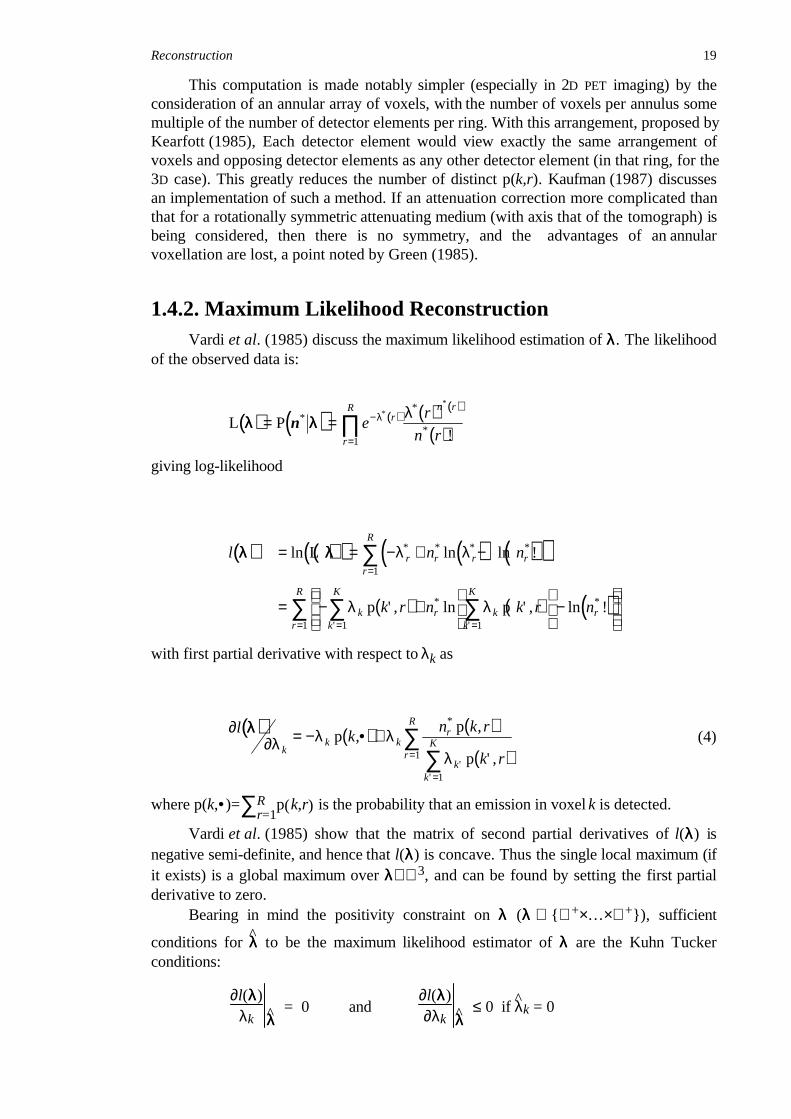
density at a point is estimated by adding all the obtained profiles through that point,effectively back-projecting each profile (i.e. sinogram pixel) across the image space andsumming. For a simple 2D object observed in two orthogonal directions, fig.12 illustratesthe approach.

Reconstruction 25

inte

nsity

first projection axis

projected intensity

backprojected intensity

Figure 12Back-projection of a point source

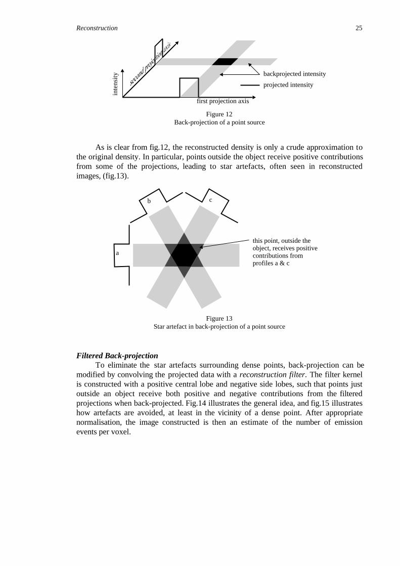
As is clear from fig.12, the reconstructed density is only a crude approximation tothe original density. In particular, points outside the object receive positive contributionsfrom some of the projections, leading to star artefacts, often seen in reconstructedimages, (fig.13).

a

b c

this point, outside theobject, receives positivecontributions fromprofiles a & c

Figure 13Star artefact in back-projection of a point source

Filtered Back-projectionTo eliminate the star artefacts surrounding dense points, back-projection can be

modified by convolving the projected data with a reconstruction filter. The filter kernelis constructed with a positive central lobe and negative side lobes, such that points justoutside an object receive both positive and negative contributions from the filteredprojections when back-projected. Fig.14 illustrates the general idea, and fig.15 illustrateshow artefacts are avoided, at least in the vicinity of a dense point. After appropriatenormalisation, the image constructed is then an estimate of the number of emissionevents per voxel.


inte

nsity

first projection axis filtered projected intensity

backprojected intensity

Figure 14Filtered back-projection of a point source

a

b c

this point, outside theobject, receives positivecontributions fromprofiles a & b, and anoffsetting negativecontribution from profile c

Figure 15Artefacts in filtered back-projection of a point source

For a more mathematical description, the reader is referred to the paper by Shepp& Kruskal in American Mathematical Monthly (1978). Most papers reviewing PET givesimilar descriptions of filtered back-projection (Ter-Pogossian et al., 1980;Raichle, 1983b).

3D filtered backprojectionIn theory, 3D FBP is a simple extension of the 2D case. In practice there are a

number of problems in implementing FBP for PET data acquired in 3D mode.A projection is complete if profiles are available for all lines that pass through the

region of interest (brain) in the direction of projection (given the discreteness of thesampling). If all projections are filtered with the same kernel, then to realise theadvantages of FBP it is necessary to have a full set of complete projections, that iscomplete projections for all possible angles (given the discreteness of the sampling). For2D reconstruction, the necessary information to reconstruct a plane is contained in thecorresponding direct-plane (or induced-plane) sinogram. In 3D PET many of the possibleprojection angles are unobservable because of the tomograph geometry. Furthermore,many of the projections that are possible are incomplete, since oblique projectionsbecome increasingly truncated as the direction of projection nears the axis of thetomograph.

Careful choice of filters for each projection (compared by Defrise et al., 1989)enables artefact-free FBP reconstruction for (incomplete) sets of complete projections.Defrise et al. (1990) discuss filtered back-projection for such data.

Reconstruction 27

To obtain complete projections it is necessary to estimate the missing profiles inpartially observed projections. This is done by reconstructing the density in 2D mode,using only the direct (and induced) plane sinograms, and obtaining the missing profilesfrom this rough estimate of the actual density. The effect is to artificially extend the axialextent of the scanner by adding extra rings of detectors. The estimated sinograms forthese artificial rings are termed synthetic sinograms. Typically the number of syntheticsinograms is comparable with the number actually observed.

Townsend et al. (1991) discuss the implementation of filtered back-projection for3D PET data acquired on the CTI-953B, a tomograph with retractable septa. Theprocedure requires the following steps: (Taken from Townsend et al., 1991, to which thereader is referred for additional details.)

1) Acquire 2D, septa-extended blank and transmission scans, and a 3D,septa-retracted emission scan.

2) Normalise the 256 emission sinograms using coefficients obtained fromthe high statistics, septa-extended blank scan.

3) Reconstruct the 2D attenuation map and forward project to obtainoblique correction factors.

4) Subtract the estimated scatter from the emission sinograms.

5) Correct the scatter corrected emission sinograms for attenuation.

6) Reconstruct (in 2D) the emission sinograms for ring differences of0 & ±2 (direct plane) and ±1 & ±3 (cross plane).

7) Forward project the sinogram corresponding to the measured sinogramwith the maximum activity, and compare (fit) with the measurement toobtain the scaling factors between the forward projected and measuredsinograms.

8) Forward project the unmeasured sinograms for all ring indexdifferences required for the reconstruction.

9) Scale the forward projected sinograms using the coefficients obtainedin step (7).

10) Form complete 2D projections and apply the appropriate filter.

11) Back-project all VORs, both measured and synthetic.

12) Re-scale the reconstructed values to counts/second/voxel.

1.4.3.4. Comments on filtered back-projection

There are two appealing properties of the filtered back-projection approach forestimating the average emission intensity for PET data. Firstly, the method is linear, soadditive corrections to sinograms can equivalently be applied to reconstructed images,after the corrections have themselves been reconstructed. Secondly, the method isanalytic, and doesn’t rely on iterative implementations. Even so, a 3D reconstruction ofone scan from the CTI-953B takes 3.3 hours on a SUN SPARCStation2(Townsend et al., 1991).

We have already noted two inadequacies of the filtered back-projection approach,namely the simplification of the emission tomography problem to the transmission


framework, and the use of VOR counts as good estimates of their means without recourseto any probability modelling.

1.4.4. Reconstructed images

Co-ordinate systems: Tomograph axesThe Cartesian co-ordinate system of reconstructed PET images is fixed relative to

the tomograph. Looking into the patient port of the tomograph; the X-axis is horizontal,running from right to left; the Y-axis is vertical, running from below to above; and the Z-axis is horizontal, running directly away from you along the axis of the tomograph. Thusfor a subject placed in the tomograph head first and on their back, the X-axis runs(roughly) from their left to their right, the Y-axis from their back to their front, and the Z-axis from their toe to their head. The origin is placed arbitrarily on the tomograph axis,and the axes are scaled in millimetres. Fig.16 illustrates the positioning and orientation ofthe axes.

x

z

y

Figure 16Positioning and orientation of tomograph axes

Planes of PET images3D images are usually viewed as a set of 2D images which form the 3D image when

stacked one on top of the other. The 2D images most frequently presented are transaxialslices, planes parallel to the XY plane. Saggital and coronal sections are planes parallel tothe YZ plane and XZ plane respectively.

Transverse sections are presented viewed from above and behind the subject: Theposterior of the brain is at the bottom of the image, the subjects left at the left side of theimage, and the X and Y axes are in their usual positions. Saggital sections are presentedviewed from the subjects right with the brain upright: The posterior of the brain at theleft of the image and the top of the brain at the top of the image. (Posterior) Coronalsections are viewed from behind the subject, with the subjects left on the left of theimage.

FBP reconstructed imageAt the MRC Cyclotron Unit at the Hammersmith Hospital in London, scans are

routinely reconstructed using three-dimensional filtered back-projection with a Hanningfilter cut off at 0.5 cycles per voxel. The discretisation of Ξ for reconstruction is of

Reconstruction 29

128×128×31 cuboid voxels of dimensions 2.09×2.09×3.5mm3 (x×y×z), with voxel edgesparallel to the tomograph axes. The resulting images are then re-sampled axially to give128×128×43 approximately cubic voxels of dimension 2.09×2.09×2.09mm3.

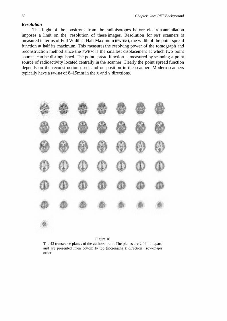
Orthogonal sections through such an image are shown in fig.17. The subject (theauthor) was injected with [15O]water and emissions recorded according to the protocoldescribed below (§1.6.1.2.). The full 43 transverse planes are shown in Fig.18.Reconstruction artefacts can be seen in the lower planes.

Col

our

Sca

le

−1 0 10

0.01

0.02

0.03

Saggital Section − x=0

z

y

−20 0 20 40

−100

−50

0

50

100

Coronal Section − y=0

z

−100 −50 0 50 100

−200

2040

Transverse Section − z=0

x

y

−100 −50 0 50 100

−100

−50

0

50

100

Figure 17Orthogonal sections of the author’s brain.

Colour scale in (estimated) annihilations per second.Tomograph axes, graduated in mm.


ResolutionThe flight of the positrons from the radioisotopes before electron annihilation

imposes a limit on the resolution of these images. Resolution for PET scanners ismeasured in terms of Full Width at Half Maximum (FWHM), the width of the point spreadfunction at half its maximum. This measures the resolving power of the tomograph andreconstruction method since the FWHM is the smallest displacement at which two pointsources can be distinguished. The point spread function is measured by scanning a pointsource of radioactivity located centrally in the scanner. Clearly the point spread functiondepends on the reconstruction used, and on position in the scanner. Modern scannerstypically have a FWHM of 8–15mm in the X and Y directions.

Figure 18The 43 transverse planes of the authors brain. The planes are 2.09mm apart,and are presented from bottom to top (increasing Z direction), row-majororder.

Tracer and Modelling Issues 31

1.5. Tracer and Modelling Issues

1.5.1. Radioactive isotopes and labellingThe radiotracers used in Positron Emission Tomography are chosen to enable the

study of particular metabolic and physiological processes in the living body. Threepositron emitting radioactive isotopes of particular use are oxygen 15 (15O), nitrogen 13(13N) and carbon 11 (11C) (Ter-Pogossian et al., 1990), with half lives of 123, 598 and1220 seconds respectively (Tennent, 1971). These isotopes are particularly valuablebecause biological systems consist mainly of compounds of oxygen, nitrogen and carbon.Labelling a biochemical, by replacing one of its atoms with a radioactive isotope, enablesimaging of the density of the labelled compound, and hence non-invasive measurement ofmetabolic processes in the living body.

Observable metabolic functionsUsing these four radioactive isotopes in different biological compounds, the

quantitative study of many facets of metabolism is possible. Among the quantities it ispossible to measure are: blood flow, blood volume, organ perfusion, brain permeabilityto various amino acids, tumour drug levels, tissue pH, tissue lipid content, heartmetabolism, tissue hematocrit (ratio of cells to plasma), mapping of monoamine oxidasereceptors (lung), neuroreceptor pharmacology (brain) and tissue drug levels in epilepsy.See Raichle (1983b) for a more detailed summary of Positron Emission Tomography andits research and clinical applications.

1.5.2. Short half lives and low activities of the isotopes

Implications for applicationThe short half lives of the radio isotopes used limit the use of PET to imaging fairly

fast metabolic processes. Fortunately the overwhelming majority of brain metabolicprocesses have proved to be fast relative to the radionuclide half-lives. The low activityof commonly used tracers forces each scan to be acquired over a period of a fewminutes. This precludes the use of PET to study very fast metabolic processes, orprocesses that are quickly reversed (in that the labelled metabolite is cleared away).

Multiple scans on healthy subjectsThe low dose of radioactivity required for a single PET scan is well below the

maximum allowable for volunteers in medical research11. Thus healthy subjects can beexamined using PET, allowing investigation of normal function. This is in contrast tomany areas of medical research, where knowledge is acquired from patients who are illor are undergoing other forms of treatment. More importantly, the low doses permitrepeat scanning of an individual. Short half-lives allow repeat scanning within a shorttime, making it feasible to obtain multiple scans on a single subject in a single session, so 11In the European community, the maximum activity that can be administered to volunteers in medicalscience is 5 milli-Sieverts per year, roughly equivalent to two years background activity. For a typical(3D) PET scan using the tracer H2

15O only about a twelfth of this amount need be injected per scan.(Source: RSJ Frackowiak, MRC Cyclotron Unit.) In the USA, the maximum allowable activity foradministration to volunteers in medical science is much higher than in the UK. Fourteen run experimentsare commonplace there, but more could be performed. The limiting factor on the number of possiblescans is the length of time a subject can spend in the scanner.


avoiding long term time differences. The multiple scans of a subject under similar ordifferent conditions permit the investigation of clinical questions within an individual. Ina statistical sense, subjects can act as their own controls.

1.5.3. Cost of PET

The development of PET was hampered by the short half lives of the positronemitting isotopes most useful for labelling. Fast methods for creating the isotopes andthen binding them into the relevant biochemicals are needed. Production must be on-site,requiring a cyclotron, and a resident team of radio-chemists. Cyclotrons for this purposetypically accelerate protons up to an energy of 15 million electron volts (MeV) anddeuterons (heavy hydrogen nuclei) up to half that energy. Such apparatus weighs sometwenty tons, is shielded by several feet of concrete. With the cost of a tomograph lying inthe region of a million pounds, PET is a very expensive imaging modality. Currently(1992) there are only about 40 centres world-wide.

1.5.4. ModellingSo far we have only considered using PET to estimate the regional activity (rA) of

the radioactive isotope administered to the subject. A study that seeks only to identifythe site of a focal abnormality in an individual, for example a tumour or infarctcharacterised by abnormally low activity, might be complete at this stage with no needfor further processing.

To quantitatively obtain measurements of metabolic function it is necessary tomodel the relationship between the tracer activity, and the metabolic parameter ofinterest. Even in comparative studies it is usually necessary to convert “counts” imagesto appropriate biological parameters, because of global differences in tracer uptake fromperson to person, or even from scan to scan in the same individual. The principles oftracer kinetic modelling are presented in depth by Huang & Phelps (1986). A briefreview from a statistical perspective is given by McColl et al. (1994, §3).

Compartmental modelsThe link between regional tracer concentration (estimated from the measurements

of radioactivity) and biological parameters is usually provided by compartmentalmodelling. These tracer-kinetic models represent each stage in the relevant biologicalprocess as a compartment. Differential equations describe the flow of the metabolite ofinterest (and its labelled analogue) between the compartments. The parameters of thesedifferential equations are those of the metabolic process of interest, and can be estimatedgiven the tracer concentration and additional physiological parameters. Typically theconcentration of the tracer in the blood pool is needed, requiring sampling of the subjectsblood during the scanning session via an arterial catheter. Such a model is applied foreach voxel of the reconstructed PET image, giving parametric images, each voxel havingvalue the estimated metabolic parameter of interest.

1.5.5. Imaging cerebral blood flowParticularly important is the measurement of regional Cerebral Blood Flow (rCBF).

The method is due to Kety (1951), and was adapted for PET by Herscovitch et al. (1983)and Raichle et al. (1983a). A simple one compartment model describes the relationshipbetween regional cerebral blood flow, the arterial (plasma) concentration of a freely

Tracer and Modelling Issues 33

diffusible blood flow tracer (measured by arterial sampling), and the total tissue/plasmaactivity (measured by PET).

Freely diffusible blood flow tracers[15O]Water is commonly used as a freely diffusible blood flow tracer. Although

H215O has only limited diffusibility, it is usually used by most PET centres in preference

to truly freely diffusible blood flow tracers such as [11C]butanol. The water method givesslight underestimates of rCBF when compared to Butanol, as noted byHerscovitch et al. (1987). However, [15O]water is easy to make to a specified activity,using a relatively cheap, low energy cyclotron. Further, [15O]water has a short enoughhalf life (123 seconds) that a subject can be repeatedly scanned with only a five minutewash-out period, without cumbersome schemes to account for residual activity.

Use of “counts” images.Conversion from local radiotracer density to local cerebral blood flow requires

arterial sampling of the blood radioactivity levels at given intervals, so that the timeactivity curve for the tracer in the cerebral plasma can be estimated. This requires theinsertion of a cannula into an artery. The cannula can become quite painful by the end ofa three hour scanning session, and the pain may dominate the subjects thoughts,compromising experiments where rCBF is being measured as an indicator of mentalactivity.

However, if the amount of tracer administered is carefully controlled, then over thenormal range of tracer uptake by the plasma, and for a fixed global CBF, the relationshipbetween regional activity (measured by PET) and rCBF is fairly linear. Thus the modellingand conversion of “counts”, or regional activity (rA) images to quantitative rCBF imagesis frequently not carried out when rCBF images are to be compared for relative changes(Mazziotta et al., 1985; Fox et al., 1989).

In fact, Mazziotta et al. (1985) report that the relationship between flow andcounts is slightly convex, so changes in regional activity are slightly conservativeindicators of changes in rCBF.


1.6. Functional Mapping with PET

The investigation of the functional organisation of the brain is termed functionalmapping. The use of PET in functional mapping experiments has matured over the pasttwo decades to the point where it is now regarded as a mature research tool.

1.6.1. Imaging brain activityEarly research into the workings of the brain showed that the brain is very well

organised, specific different tasks being dealt with by specific physical areas of the brain.With Positron Emission Tomography the physical locations of function in the humanbrain can be identified by using a radiotracer whose density reflects local brain activity.

Electrical neuronal activityThe brain works by communication between neurones using small electrical

currents, generated and transmitted by chemical reactions (Fishbach, 1993). Localneuronal electrical activity is thus the absolute measure of local brain activity. Earlymethods measured this directly, using electrodes placed on the scalp(electroencephalogram) or even in the brain itself.

1.6.1.1. Tracers for functional mapping

Metabolic activity induced by neuronal activityIncreased neuronal (electrical) activity causes an increase in metabolic activity for

maintenance of the neuronal membrane ionic gradients (Yarowsky et al., 1981). Undernormal conditions the brain uses glucose and oxygen as energy substrates(Phelps et al., 1986, ch1)12. By examining the metabolism of these substrates using PET,the activity of the human brain can be observed. The regional cerebral metabolic rate ofoxygen (rMRO2) is the most direct measure of regional energy metabolism, but this ishard to measure. The regional cerebral metabolic rate of glucose (rCMRG) can bemeasured by labelling an analogue of glucose, deoxyglucose, which follows the samemetabolic pathways until the blood-brain barrier has been crossed, and is then effectivelytrapped in the brain (for a short time). Experiments in rats and monkeys usingautoradiography13 dramatically illustrate the relationship between physiological functionand energy metabolism in the brain (Sokoloff, 1979). The deoxyglucose method has beenused successfully in man with PET, using 18F as a label. However, scanning requires a 30minute equilibration period, during which time patterns of neuronal activity may changesubstantially. Also, repeat scanning of a subject on the same day isn’t possible, becauseof the long half-life of 18F (110 minutes). Usually fluoro-deoxyglucose (FDG) is used indynamic scans, where a sequence of sequential scans are acquired after the introductionof the tracer, and its progress through the brain examined over the time course of theexperiment. A more efficient method to study mental activity is via rCBF.

12The brain is one of the most active organs metabolically in the body. Although comprising only c2%of the total body weight, it accounts for c20% of the total body oxygen consumption (at rest), andmaintains a power output of at least 20 watts (Phelps et al., 1986, ch1).13 In autoradiography (AR) a laboratory animal is injected with a radiotracer, decapitated, and theirfrozen brain sliced and placed on photographic film to obtain precise images of radiotracer density.

Functional Mapping with PET 35

rCBF as indicator of regional neuronal activityThe brain has almost negligible stores of energy substrates when compared their

rates of utilisation, and is hence dependent on blood circulation to supply its needs.Complete interruption of cerebral circulation leads to loss of consciousness within 10seconds, and irreversible brain damage within a few minutes. So great is the demand forenergy substrates that an increase in neuronal activity induces a dilation of the veins inthe vicinity, in turn increasing the blood flow in the region (Kety, 1991). This inducedincrease in rCBF lags behind the neuronal activity by mere seconds.

Thus, PET measurements of rCBF, or rA as an indicator of rCBF, are indicative of theaverage neuronal activity over the period of the acquisition. The “average” here beingweighted by the activity of the tracer, and hence emphasising the neuronal activity at thebeginning of the acquisition period.

1.6.1.2. H215O infusion protocol

There are many different protocols for acquiring scanning using [15O]water. Forroutine studies at the MRC Cyclotron Unit (Hammersmith Hospital, London) on the 953Bdedicated brain positron tomograph, the following protocol has been adopted(Bailey et al., 1993)

Scanning protocolThe subject is positioned in the scanner, using external landmarks to obtain rough

alignment, and a 2D transmission scan acquired for attenuation correction procedures. (Ablank scan having been made at the beginning of the day.) A thin indwelling cannula fortracer administration is inserted into a superficial vein in the right forearm. After thetransmission scan the inter-plane septa are removed to allow 3D acquisition of theemission scans. For each scan, H2

15O is infused via the cannula at a constant rate of10ml/min. The task is initiated at the commencement of data acquisition, which consistsof a 60s background frame, at the end of which tracer administration is started. The datais acquired in a single 3D frame for 150s. The infusion is terminated after 120s, theacquisition continuing for a further 30s. In each run approximately 1040 MBq (28 mCi)of [15O]water is administered. Emission scans are acquired every 12 minutes, to allowfor tracer washout and decay, and 12 scans are acquired in the session.

Infusion systemThe infusion system consists of a small furnace containing a palladium catalyst over

which 15O2 (from the cyclotron) is passed as a dilute (1:99) mixture in nitrogen. The hotH2

15O vapour produced is passed across one side of a cellulose acetate semi-permeablemembrane. Isotonic saline, driven be a conventional medical infusion pump, is passedacross the other side of the membrane and the H2

15O transfers into the saline. Thedevice is compact and sits under the tomograph patient bed. A calibrated Geiger counteris incorporated into the infusion system to monitor accurately the amount of radioactivityinfused. When not switched to the subject, H2

15O is drained into a lead encasedreservoir. The constant production of H2

15O helps achieve a stable, reproducibledelivery of tracer as the system settles into a constant pattern.


1.6.2. Types of studyMost PET functional mapping experiments take one of a few forms.

1.6.2.1. Common factors

All functional mapping experiments using PET have common factors dictated by theconstraints of the technique.

ComparativeDistinct parts of the brain naturally have different activity and rCBF, so functional

mapping experiments must proceed by comparing rCBF (rA). The 3D PET H215O method

allows for each subject to be scanned numerous times in a three hour scanning session.Subjects can therefore be scanned repeatedly under the mental conditions of interest, andact as their own controls.

Multi-scanChanges in rCBF induced by neuronal activity are very subtle, typically at most

10%, and are dominated by the noise in the reconstructed images. Increases in rCBF

between a “rest” task and an “activation” task are not readily apparent in reconstructedimages taken under the two conditions. It is necessary to obtain repeat observations andapply statistical tests. For some basic functions the changes in rCBF can be seen in asingle individual scanned 12 times using the 3D PET H2

15O method. With less sensitive2D acquisition, more subtle activations or more complicated protocols it is necessary topool rCBF data across individuals to reliably detect rCBF changes. When it is desired tomake deductions about a population rather than an individual, it is necessary to scan asample of individuals from the population.

Small subject numbersPET scanning is expensive. A three hour, 12 scan PET session costs in the region of

two thousand pounds (Sterling). For this reason, sample sizes are very small. The largeststudies completed to date have only 12 to 14 subjects. Typically only 6 subjects will takepart in a study.

Single subject studiesWith the increasing sensitivity of scanners, better reconstruction and more sensitive

statistical procedures, significant results can be obtained on a single subject. This has ledto move to “single subject” studies. Often interest lies in the individual: “Where is thebrain gyrus in this individual which initiates motion in the right index finger?” However,in many single subject experiments the subject is assumed to be representative of thepopulation and the results accepted for that population.

No prior informationKnowledge of the functional specialisation of the human brain is still limited, and

even basic tasks have only recently been mapped. This lack of prior knowledge regardingthe location of function necessitates the consideration of the whole brain volume, or theuse of hypothesis generating experiments before a full study examining condition inducedchanges in rCBF at hypothesised locations. The expense of PET leads researchers to adoptthe former approach, trying to get the most out of the data they have, placing emphasison good statistical procedures to analyse these data sets.


1.6.2.2. Activation studies

The simplest and commonest paradigm is the activation study, designed toaccurately locate the brain region responsible for performing a particular cognitive task.Subjects are scanned under two conditions, a baseline or “rest” condition, and“activation” condition, carefully chosen by the experimenter on psychological groundssuch that the mental processing required by the two conditions differs only in thecognitive task it is wished to locate. Localised changes in measured rCBF between thetwo scans are due to natural variation, scanner noise, or are induced by different patternsof neuronal engagement. The problem is to identify changes that fall into the lattercategory. Usually arterial sampling is not carried out, and images of regional activity areanalysed as indicators of regional neuronal activity.

Most experiments are concerned with mapping simple tasks. The somatosensorycortex is readily mapped by activation studies, using a rest baseline, and a simple sensorystimulation as the activation condition. Similarly the motor cortex is easily mapped.Contrasting a rest baseline condition with an activation condition where the subjectrepeatedly extends a finger identifies the brain region responsible for control of thefinger.

In a simple activation experiment, only two conditions are used. The aim is toreliably locate a particular task. In a compound activation study, several conditions areused. Interest may lie in the difference in neuronal engagement between many conditions,or many activation conditions might be compared with a single baseline condition in ahypothesis generating experiment.

Typical experimentThe typical simple activation study will have four, six, or twelve right handed male

volunteers between the ages of 25 and 50 years. Each subject is scanned twelve times ina single session, each scan under either the baseline or the activation condition. Theconditions are assigned to the scan times for each subject before the scanning session.Usually the allocation is balanced, but not necessarily random. Typically subjects will bescanned alternately under the two conditions, with half the subjects starting with thebaseline condition for scan one, the remaining half starting with the activation condition.This gives a one-way block design with replication, where the blocks are the subjects,and the data points are images of rA or rCBF.

Single subject activation studies are not usually performed explicitly. Ratheractivation studies are performed and the subjects considered individually as well as agroup.

1.6.2.3. Correlation with an external variable

It is not always possible to design conditions inducing mental states differing onlyin the cognitive component it is wished to locate. Sometimes it is wished to locate a brainregion which is increasingly engaged as the severity of some task increases. In many ofthese situations it is possible to obtain a score, indicating the severity of the task.Assuming a linear relationship between rCBF and the score, the regions increasinglyengaged by the tasks can be identified as those with rCBF and score highly positivelycorrelated. These studies are referred to as correlational studies. There are a twovariants, across subjects, and within and across subjects.

Across subjectsThis paradigm is typically used to locate the brain region whose function is

impaired by a particular disease. A number of sufferers with varying degrees of


debilitation are scanned whilst performing the task the disease impairs. The scores areclinical scores reflecting the severity of the disease. The location of the function whichworsens with the onset of the disease may be found as those regions where rCBF

correlates negatively with the score. These studies are particularly prone to changes inglobal CBF, and different normalisation schemes can result in different results, a pointillustrated by McCrory & Ford (1991).

Within & across subjectsAlternatively, interest may lie in locating the brain regions increasingly engaged by

progressively more difficult tasks. Subjects are scanned a number of times whilstundertaking a task, each subject performing the task at various levels of difficulty. Thescore for each scan is then simply either a measure of the task difficulty, or a measure ofthe subjects performance. The regions increasingly engaged by the task are located asthose whose rCBF correlates positively with the scan score.

An example of this approach is a study where 12 subjects were scanned whilstattempting to remember lists of words. During each scan, word lists of given length werepresented verbally by the experimenter, for immediate recall. Over the 12 scans eachsubject faced list lengths from 3 to 14 words in length, the actual order of allocation oflist lengths to scans for each subject having been made randomly. The score for eachscan is simply the length of the word lists presented during that scan. Regionsincreasingly engaged in longer term memory tasks should have rCBF highly correlatedwith score.

1.6.2.4. Cross group comparison

Other studies seek differences in function between groups. Typically a group ofnormal volunteers are compared with a group of patients suffering under some conditionaffecting their mental performance. Each group undergoes an activation study, anddifferences in response between the groups are sought.

1.6.2.5. Flow correlation, Functional connectivity

So far we have only considered experimental paradigms for locating particularfunctional centres in the brain. The brain can be thought of as a large and complexnetwork of interconnected neurons. There are known neuronal projections between brainregions which are physically far apart. These connections should manifest themselves inPET data as correlations in the rCBF measurements of different regions. Recent efforts infunctional brain mapping have sought to locate these connections, examining sequencesof rCBF scans for correlation. These experiments are known as functional connectivityexperiments .

Occasionally it is desired to locate the brain loci functionally connected to a knownregion. In this situation correlations between the rCBF of the hypothesised region and allother regions can easily be computed, and subsequently examined. Frequently there is nohypothesised primary brain loci. In these situations factor analytic approaches are beingdeveloped to elucidate the correlation structure.

1.6.3. Region of interest methodsThere are two broad classes of analysis methods employed for PET data, Region of

Interest (ROI) approaches and voxel-by-voxel approaches.


1.6.3.1. ROI methods

In ROI approaches, anatomical regions which are of interest are defined. Theseanatomical regions are identified on the PET scans. The average rCBF in each of theregions is calculated, usually by taking the mean value of the voxels inside the region.This results in a large reduction in the dimensionality of the data set. A typical rCBF

image consists of approximately 77000 voxels, whereas typically only tens of ROI aredefined.

ROI identification–Hypothesis generationUsually the ROI are chosen with a particular hypothesis in mind. The functional

anatomy of monkeys has been extensively studied using autoradiography, so regions ofthe human brain corresponding to those of the monkey whose function is known may bechosen in an experiment hoping to extend monkey results to humans. Alternatively, pilotstudies or previous experiments may have suggested that a particular region beimplicated in a certain task. Occasionally, the whole brain is partitioned into many smallregions of interest, identified on anatomical grounds (Mazoyer et al., 1993).

AnalysisWhen there are a selection of regions of interest, standard multivariate procedures

have been applied. However, there are many problems, as indicated byFord et al. (1991). The small sample sizes of functional mapping experiments results indata where often there are more ROI than there are replications. This results in a singularsample correlation matrix, precluding the use of many multivariate procedures.

When interest is in a particular region, a simple univariate statistical procedure canbe used. With many ROI statistical testing can be performed on a region-by-region basis,using univariate techniques at each region. This approach is possibly more robust thanthe multivariate methods, though may be excessively conservative once adjustments forthe many multiple comparisons have been made. An advantage of applying simpleunivariate statistical procedures is that medical researchers are more likely to be familiarwith them.

DiscussionThe review of Ford et al. (1991) discusses many of the statistical problems with

ROI analyses, illustrated with real data sets from a variety of experiments. Section 4 ofMcColl et al. (1994) brings a review of ROI analyses up to date.

Many of the issues in ROI analysis are of concern in voxel-by-voxel methods, towhich we now turn.

1.6.4. Voxel-by-voxel methods of analysis

1.6.4.1. Overview

The smallest brain region that can be defined for an image is that corresponding toa single voxel. Defining each voxel as a ROI also gives the highest resolution possible forlocating a functional component. In the absence of any prior hypothesis regarding theexpected location of the particular function under study, voxel ROI provide theframework for the most general analysis. These approaches are termed voxel-by-voxelmethods.


Statistic imagesVoxel-by-voxel approaches proceed by analysing the data for each voxel across the

data using univariate techniques. This results in the computation of a statistic for eachvoxel, giving statistic images. The significance of these statistic images must then beassessed. Several schemes to account for the multiplicity of testing in this special spatialsetting have been derived.

The formation and analysis of statistic images from activation experiments are theprime topics of this thesis. In chapters 2 and 3 we review current methods forformulating and assessing the significance of statistic images for PET functional mappingexperiments. In the remainder of the thesis we consider new methods for assessing thesignificance of statistic images.

1.6.4.2. Re-alignment

Clearly for a voxel-by-voxel analysis it is imperative that the images obtained be inalignment, such that any particular voxel location corresponds to the same physical braingyrus for all images.

During the course of a three hour scanning session, the subject is certain to moveabout on the scanner bed. This motion can be minimised by the use of custom made headholders and other restraints. These are rather uncomfortable if the head is held toorigidly, and may be distressing to the subject (fig.19). As it is the subjects thoughts thatare of prime interest in activation studies, restraint must be as unobtrusive as possible,and most head restraints allow some movement. Subjects are encouraged to remainmotionless for the duration of each scan, to prevent blurring the acquisition. Laser beamsare often mounted on the tomograph gantry, and are aligned with lines drawn on thesubjects head, enabling repositioning to approximately the same position at the start ofeach scan. This precaution helps minimise changes in head position and orientationrelative to the tomograph between scans.

Figure 19A (rather severe) head holder


Despite these precautions, motion between scans is likely, leading to mis-registration of the reconstructed images. To correct these translational and rotationalmotions various realignment procedures have been developed.

Image alignmentTo align two images the co-ordinate axes of one must be rotated and translated to

match the anatomical position and orientation of the axes in the other image. Thistransformation is parameterised by three rotational and three translational parameters.The new co-ordinate axes can be obtained by a rotation of θ about the z-axis, a rotationof φ about the y-axis, and a rotation of ψ about the x-axis, followed by a translation ofthe origin to point o' = (o'x,o'y,o'z)

T.If the new axes are O'X', O'Y' and O'Z', then the co-ordinates of point (x,y,z)T

relative to these new axes are (x',y',z')T relative to the old axes, where:

x'y'z'

=

cosφcosθ cosφsinθ -sinθ

sinψsinφcosθ-cosψsinθ cosψcosθ+sinψsinφsinθ sinψcosφsinψsinθ+cosψsinφcosθ cosψsinφsinθ-sinψcosθ cosψcosφ

xyz

+

o'xo'yo'z

x' = RXYZ x + o'Eqn.(10)

Eqn.10 is a function of six parameters, three rotation angles and three translationdistances. These parameters are known as the reslice parameters (Woods et al., 1992).

Once the reslice parameters have been estimated for an image A=(A1,…,AK), theimage can be aligned to the new axes O'X' O'Y' O'Z' by re-sampling the image, using tri-linear interpolation14 to give new image A'=(A'1,…,A'K) with cuboid voxels aligned withthe (new) axes. Point x' in the reoriented co-ordinates corresponds to RXYZ

-1(x'-o') in theoriginal co-ordinates.

Once two images from the same subject have been aligned, the same voxel fromeach image corresponds to the same volume of brain.

Estimation of reslice parameters: Fiducial MarkersVarious methods have been devised to estimate the reslice parameters. Usually,

one image is chosen as a reference image, and other images (reslice images) are alignedto it.

The simplest methods for realigning involve the use of fiducial markers whosepositions are fixed relative to the subjects head. If radioactive markers are used then themarkers show up on reconstructed images, and aligning the markers aligns the brainimages. The reslice parameters satisfy x' = RXYZ x + t (eqn.10) with x' the co-ordinates ofa marker in the reference image and x the co-ordinates of the same marker in the resliceimage. With three (non-collinear) markers the resulting simultaneous equations can besolved for the reslice parameters (θ,φ,ψ,tx,ty,tz). These methods are rather crude, mustbe applied prospectively, and involve additional radiation exposure for the subject. Thusmathematical image alignment methods that can be applied retrospectively have beeninvestigated.

Estimation of reslice parameters: Mis-alignment score methodsThese methods for realigning two images proceed by minimising some mis-

alignment cost function with respect to the reslice parameters. The reslice image is re-sampled with the reslice parameters that minimise the mis-alignment cost.

14Tri-linear interpolation is described fully in appendix A:2.


The cost functions proposed rely on the observation that two rCBF images on thesame subject are similar, up to a scale factor (due to global changes), noise, and somelocalised (small) condition specific change. Mintun & Lee (1990) first applied thisapproach, using the stochastic sign change criterion (SSC) to provide a cost function. Themisalignment cost function is computed as the number of sign changes (zero crossings)in the subtraction image formed by subtracting from the reference image the re-sampledreslice image for the current reslice parameters. When the images are aligned, thesubtraction image should be mainly random noise and the number of sign changes large.The reslice parameters are sought as those maximising the number of sign changes.Minoshima et al. (1992) found this method sensitive to small global changes.

Eberl et al. (1993) used the downhill Simplex multidimensional minimisationtechnique to find reslice parameters minimising a misalignment cost function formed bysumming the absolute difference in voxel values between the two images. This was foundto be substantially more accurate than the SSC method, and robust to changes in gCBF.

Woods et al. (1992) developed a similar method that has become the standardrealignment procedure, because of the availability of good software that has receivedextensive empirical validation. A proportional model is used, the idealised assumptionbeing that when the two images are aligned, the value of any voxel in the reference imageis roughly related to the value of the corresponding voxel in the reslice image by a singlemultiplicative factor. The misalignment cost function is the sample variance (computedover all voxels) of the ratio of the two scans.

With the emergence of single subject studies, there has been a move towards theuse of superimposed anatomical MRI images of the same subject. To co-register the PET

and MRI images, modifications of the various alignment techniques are used, the mostsuccessful being that of Woods et al. (1993b).

1.6.4.3. Anatomical normalisation

No two brains are physically identical, but the basic gyral anatomy (topology) isidentical, and functions are tied to a particular gyrus. Since corresponding voxels inimages of two different subjects will not correspond to the same brain gyrus, some formof anatomical normalisation is needed rectify this before analysis of images acrosssubjects on a voxel-by-voxel basis. This normalisation is termed stereotacticnormalisation.

Stereotactic atlas, reference brainsTo standardise the study of neuroanatomy, various brain atlas have been proposed.

Talairach & Tournoux (1988) dissected a human brain, photographing transverse slicesonto which a co-ordinate system was overlaid and the brain gyri and lobes labelled. Thisbrain has become a reference brain for much neuroanatomy, and the Talairach co-ordinate system has become a standard for describing brain locations. Hence, even withstudies of an individual, anatomical normalisation is necessary to enable locations to bereported in standard Talairach co-ordinates.

The Talairach co-ordinate system is based on the inter-commissural or AC-PC line,the imaginary line joining the centres of the anterior and posterior commissures. Themidpoint of the AC-PC line is the origin of the Talairach co-ordinate system (fig.20). TheY-axis runs along the AC-PC line from posterior to anterior, the X-axis from (subject) leftto right, and the Z-axis from the bottom to the top of the brain. The YZ plane bisects thebrain into its two hemispheres. Co-ordinates are given in millimetres from the origin inthe axial directions. The AC-PC plane is the plane z = 0.


AC-PC line

x

z

y

Figure 20The intercommisural line, and Talairach axes

Estimation of AC-PC lineMost methods for stereotactic normalisation to Talairach co-ordinates begin by

estimating the position of the AC-PC line. Early methods relied on external landmarks,head fixation and a secondary imaging modality showing enough anatomical detail tolocate the AC-PC line by eye (Fox et al., 1985). The improvement in resolution of PET

images enabled the identification of anatomical landmarks such as the edges of theventricles.15 The positions of certain landmarks have been shown to lie near the AC-PC

line for many brains studied by MRI (Friston et al., 1989). The AC-PC line can then beestimated by regression. Once the AC-PC line is fitted, the Talairach origin is found, andthe X and Z axes located by fitting the YZ plane to bisect the brain into its twohemispheres.

Most centres now have templates for aligned PET images16 which can be comparedto the study image to estimate the AC-PC line automatically. Typical of early approachesis that of Friston et al. (1991a), as implemented in early versions of the SPM software:17

The YZ plane is located by eye as the plane bisecting the brain into its two hemispheres, aY-axis is chosen in this plane in the rough vicinity of the AC-PC line, and an originarbitrarily chosen. The image is re-sampled to these new axes. The true AC-PC line lies inthe YZ plane. To locate it, 15 coronal sections (y = constant) from the image are taken,and the height (z) of the AC-PC line in each is estimated.18 These heights are regressed onthe y values of the coronal sections, giving the estimate of the AC-PC line.

15The brain contains several hollow pockets of spinal fluid, called ventricles. The spinal fluid is virtuallyfree of tracer, and shows up black on PET scans of rCBF.16Template images are usually formed as the average of many PET scans that have been stereotacticallynormalised.17For a recent approach, see Friston et al. (1994). This is the method implemented in the SPM94software.18The height of the AC-PC line for each coronal section is estimated by comparison with the templateimage: Each section is aligned (by shift in Z-direction) with a selection of coronal sections from thetemplate, and the best fit found. The height of the AC-PC line in the template sections is known, soadding this to the Z-shift for the best fit gives the estimated height of the AC-PC line.


Stereotactic normalisationOnce the Talairach origin and axes have been located, the PET image can be aligned

to these new axes. There remains the problem of stereotactically transforming the PET

brain to the atlas brain, deforming the image about the origin so that it has the samemorphology as the Talairach brain.

The simplest methods simply scale the image in the axial directions so that theoverall brain size matches the atlas (Fox et al., 1985). After scaling the image is re-sampled to a standard resolution, typically with 2×2×4mm3 voxels. This gives astereotactical normalisation procedure with 9 degrees of freedom; the three rotations andthree translation parameters of the alignment, and three scaling parameters.

The most general linear transformation from tomograph axes to Talairach co-ordinates is effected by three-dimensional affine transformations, a general lineartransformation (except reflection or central inversion) followed by a translation(Woods et al., 1993a). If x is the position of a point on the tomograph axes then the co-ordinates after affine transformation are x' = L x + o' where L is a positive definite 3×3matrix and t the translation vector, giving a stereotactical normalisation procedure with12 degrees of freedom. Once L and o' have been estimated the image can be re-sampledinto Talairach co-ordinates with the desired voxel dimensions.

Reference brainsWoods et al. (1993a) have extended their alignment method (Woods et al., 1992)

to affine transformations, allowing anatomical normalisation to a reference brain for PET

and MRI images. This has led to studies where all images are aligned within subjects, andthen all subjects images anatomically normalised to a reference brain, either that of thefirst subject of a previously studied subject. Results are presented superimposed on theMRI of the reference brain, or on an average of the anatomically normalised subject MRIs,the blur in the latter giving some indication of variability in anatomy after normalisation.

Non-linear transformationsFriston et al. (1991c) proposed a general plastic transformation to reshape an

image to a template formed as the average of previously stereotactically normalisedimages. A continuous general re-sampling function r(x) was proposed such that point x ina one-dimensional continuous “image” a(x) corresponds to point r(x) in the standardspace. Given a template image t(x), r(•) was estimated to satisfy t(x) = a(r(x)) subject tor'(x) ≈ 1, the latter restriction reflecting the fact that the distortion should be slowlyvarying. This was applied (Friston et al., 1991a) to images previously oriented to theTalairach axes. A quadratic re-sampling function relating the heights of the image planesto the corresponding height in the template was estimated using polynomial regression,and the image volume re-sampled for this quadratically deformed Z-axis. Each transverseplane was then re-sampled to a polar co-ordinate system and deformed to match thecorresponding transverse plane from the template by estimating the general 1D re-sampling function r(•) along each radii, and re-sampling. This approach gives goodresults and has been widely used, mainly due to the availability of software as part ofolder versions of the SPM package.

1.6.4.4. Primary smoothing

Images reconstructed by filtered back-projection are quite noisy. The highest(spatial) frequency of the noise is constrained only by the reconstruction filter used(typically a Hanning filter, with cut off frequency arbitrarily chosen at 0.5 cycles per


voxel). At this point in the analysis, it is usual to smooth the images. This primarysmoothing, as it is known is applied for a number of reasons.

MotivationIn single subject experiments there are only 6–12 scans available for inference.

Changes in rCBF induced by changes in neuronal activity are quite subtle, may bedominated by the noise in any one scan, and therefore difficult to detect. In theterminology of signal processing, the noise has a high spatial frequency, and blood flow alow frequency. Smoothing the image with a low-pass filter increases the “signal-to-noise”, making changes in rCBF more easily detectable, at the expense of a loss inresolution.

In multiple subject studies there are usually enough replications that subtle changesin rCBF between conditions are detectable, provided the activation has a coherentlocation in the stereotactically normalised images. Since the alignment and anatomicalnormalisation procedures are not perfect, and since humans exhibit limited biologicalvariation in functional location, the same stimulus in different subjects will not necessarilycause rCBF changes at the same location in the anatomically normalised images. To allowfor this residual functional variability, images are smoothed by running a moving averagefilter over the voxellated image. This extends spatially the influence of the actual activityat the brain location corresponding to a particular voxel, and hence allows slightlyseparated changes in rCBF from several individuals to “constructively interfere” instatistic images.

For basic brain functions (the senses, motor control) the anatomical localisation offunction is particularly precise. Thus for the study of basic functions smoothing shouldnot be used on the grounds of functional variability alone. Further, the changes in rCBF

induced by neuronal activity in these areas quite marked, so smoothing mayunnecessarily degrade resolution. The mechanics of smoothing are discussed in appendixB.

1.6.4.5. Adjusted images

After reconstruction, alignment within subject, anatomical normalisation (ifrequired) and primary smoothing, the images are ready for a voxel-by-voxel analysis.Scans at this stage of the analysis are known as adjusted images. The same voxel fromall the images has value reflecting neuronal activity in the same functional area in each ofthe subjects, subject to some errors in realignment, anatomical normalisation and naturalbiological variability in functional specialisation.

ExampleFig.21 depicts the rCBF image of fig.17 (p29), after stereotactical normalisation

using the methods of Friston et al. (1989 & 1991a&b), and primary smoothing using aGaussian filter of width 20mm×20mm×12mm.


Col

our

Sca

le

−1 0 10

5

10

15

x 10−3

Saggital Section − x=0

z

y

−20 0 20 40 60−100

−50

0

50

Coronal Section − y=−18

z

−50 0 50

−20

0

20

40

60

Transverse Section − z=0

x

y

−50 0 50−100

−50

0

50

Figure 21Orthogonal sections of the author’s brain, after anatomical normalisationand smoothing. Colour scale in (estimated) annihilations per second pervoxel. Co-ordinates are millimetres in Talairach space.

Data Set-The "V5" Study 47

1.7. Data Set–The “V5” Study

Throughout this thesis we shall be applying the methods discussed to a real PET

data set. The functional mapping experiment we shall use is a simple activation study, the“V5” study, recently published by Watson et al. (1993), where the reader is referred forfull details of the experiment.

Data acquisitionIn brief, there were twelve normal volunteers in the study group, nine males and 3

females, with ages ranging from 21 to 70 years. Each subject was scanned twelve timesin a single 3hr scanning session, using the 3D acquisition mode of the CTI 953B PET

tomograph. 15O-Water was used as a freely diffusible blood flow tracer, infusedaccording to the protocol of §1.6.1.2. The tomograph VOR data were corrected fordetector efficiency and attenuation, and reconstructed by three-dimensional filtered back-projection with a Hanning filter cut off at 0.5 cycles per voxel. The discretisation of Ξ forreconstruction was of 128×128×31 cuboid voxels of size 2.09×2.09×3.5mm3 (x×y×z).The resulting estimated activity images had resolution 8.5×8.5×4.3 mm at Full Width atHalf Maxima (FWHM). These regional activity (rA) images were used as rCBF indicators,as arterial sampling and the subsequent quantitation to rCBF was not carried out. Imageswere realigned within each subject using software provided by Woods et al. (1992). Thebrain was identified by reference to coregistered MRI images, and other areas removedfrom the images. Thus, all voxels with rA>0 correspond to regions within the braintissue. The resulting images were transformed to the stereotactic atlas of Talairach andTournoux using the methods of Friston et al. (1989, 1991), with re-sampling to a 65×87×26 volume of 2×2×4mm3 cuboid voxels. Finally images were smoothed by convolutionwith a Gaussian kernel of FWHM 10mm×10mm×12mm to overcome functional variabilityand residual anatomical variability.

Scan conditionsThere were two conditions under which scans were acquired. During condition A

scans subjects viewed a random stationary pattern of small squares. For condition B thesquares moved smoothly in random directions. The conditions were presentedalternately, the series commencing with A in six randomly chosen subjects and B for theremaining six. The aim of the study was to identify visual area V5, the part of the visualcortex responsible for processing motion.19

AcknowledgementThe author wishes to thank JDG Watson (formerly a research fellow with the

Medical Research Council Cyclotron Unit clinical sciences section) for assistance withthe data, the Wellcome Trust for supporting the research, and S Zeki (Department ofAnatomy, University College London) and RSJ Frackowiak (MRC-CU clinical sciencessection) for permission to use the data.

19Previous autoradiographic studies of the Macaque monkey had demonstrated the specialisation ofvarious parts of the visual cortex (which takes up the whole posterior of the brain). A 2D PET study(Zeki et al., 1991) had indicated this functional specialisation was present in man, and found theapproximate location of areas V5 and V4 (the colour centre of the visual cortex). The present study wasundertaken to accurately locate area V5 in relation to the sulcal and gyral pattern of the cerebral cortex.

Andrew

Note: Page 48 intentionally left blank

chapter one pet background - wellcome trust centre for ... · chapter one pet background ......

Documents