chapter vi normed vector spacesvps/me505/iem/06 01.pdf · chapter vi normed vector spaces october...
TRANSCRIPT

Chapter VI Normed Vector Spaces October 9, 2017
429
CHAPTER VI
NORMED VECTOR SPACES
VI.1 Normed Vector Spaces
VI.2 The Generalized Fourier Series
VI.3 Eigenvalue Problem – Sturm-Liouville Theorem
VI.4 Sturm-Liouville Problem for Equation X X 0µ′′ − =
VI.5 Table “Sturm-Liouville Problem for Equation X X 0µ′′ − = ”
VI.6 Review Questions, Exercises and Examples
VI.7 More on Normed Vector Spaces – Theory and Examples
VI.8 Elements of Quantum Mechanics
Interior court of Armenian church in Lvov
Chapter VI Normed Vector Spaces October 9, 2017 430
VI.1 NORMED VECTOR SPACES The Sturm-Liouville Theorem provides the main tool for construction of the solutions of the Initial-Boundary Value Problems for PDEs. It yields the complete set of orthogonal functions { }ny which can serve as a basis for representation of the solution in the form of the
Generalized Fourier Series n nn
u c y= ∑ .
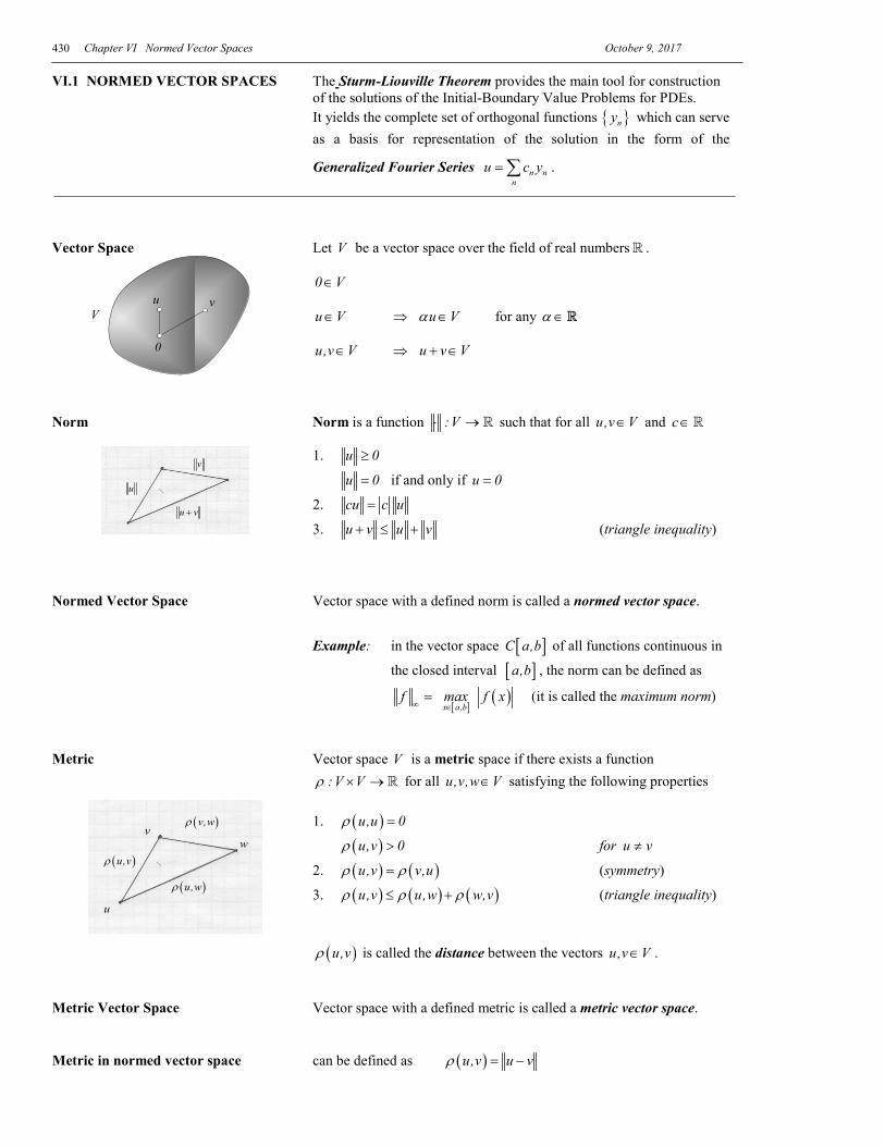
Vector Space Let V be a vector space over the field of real numbers . 0 V∈ u V∈ ⇒ u Vα ∈ for any α ∈ u,v V∈ ⇒ u v V+ ∈ Norm Norm is a function :V⋅ → such that for all u,v V∈ and c ∈
1. u 0≥
u 0= if and only if u 0=
2. cu c u=
3. u v u v+ ≤ + (triangle inequality) Normed Vector Space Vector space with a defined norm is called a normed vector space.
Example: in the vector space [ ]C a,b of all functions continuous in
the closed interval [ ]a,b , the norm can be defined as
[ ]
( )x a ,b
f max f x∞ ∈
= (it is called the maximum norm)
Metric Vector space V is a metric space if there exists a function :V Vρ × → for all u,v,w V∈ satisfying the following properties 1. ( )u,u 0ρ =
( )u,v 0ρ > for u v≠
2. ( ) ( )u,v v,uρ ρ= (symmetry)
3. ( ) ( ) ( )u,v u,w w,vρ ρ ρ≤ + (triangle inequality) ( )u,vρ is called the distance between the vectors u,v V∈ . Metric Vector Space Vector space with a defined metric is called a metric vector space. Metric in normed vector space can be defined as ( )u,v u vρ = −
u
wv
( )u,wρ
( )v,wρ
( )u,vρ
V
0
u v
v
u v+
u

Chapter VI Normed Vector Spaces October 9, 2017
431
Inner Product Inner product is a function ( ), :V V× → such that for all u,v,w V∈
1. ( ) ( )u,v v,u=
2. ( ) ( ) ( )u v,w u,w v,wα β α β+ = + ,α β ∈
3. ( )u,u 0≥
( )u,u 0= if and only if u 0= Inner product space is a vector space with a defined inner product. Norm in inner product space In an inner product space the norm can be defined as
( )u u,u= for all u V∈ Convergence in normed space Let V be a normed (metric) space and let kf , f V∈ , k 1,2,...= The sequence 1 2f , f ,... converges to f if kk
lim f f 0→∞
− = or ( )kf , f 0ρ → as k → ∞
Cauchy sequence The sequence kf V∈ is called the Cauchy sequence (convergent in itself) if k mk
m
lim f f 0→∞→∞
− = or ( )k mf , f 0ρ → as k → ∞ and m → ∞
Complete vector space The vector space V is called complete if all its Cauchy sequences kf
are convergent in V (there exists f V∈ such that kf f→ ). Banach space A complete normed space is called the Banach space. Hilbert space A complete inner product space is called the Hilbert space.
( )Stefan Banach1892 1945−( )
David Hilbert1862 1943−

Chapter VI Normed Vector Spaces October 9, 2017 432
Orthogonality The vectors u,v V∈ are called orthogonal if ( )u,v 0= If set { }ku V∈ consists of mutually orthogonal vectors ( )k mu ,u 0= when k m≠ then this set is called an orthogonal set. In addition, if k u 1= , then set { }ku V∈ is called orthonormal:
( )k m km
1 if k mu ,u
0 if k mδ
== = ≠
Vector Space ( )2L a,b Consider the set of all functions ( )xϕ defined on the interval ( )a,b
such that their square ( )2 xϕ is an integrable function over ( )a,b :
( ) ( ) ( ) = → < ∞
∫
b2 2
a
L a,b : a,b such that x dxϕ ϕ
Introduce the inner products in vector space ( )2L a,b .
For ( )2u,v L a,b∈ define:
( ) ( ) ( )b
a
u,v u x v x dx= ∫ inner product in ( )2L a,b
( ) ( ) ( ) ( )b
pa
u,v u x v x p x dx= ∫ weighted inner product in ( )2L a,b
with the weight function ( )p x 0> Defined inner products induce the norms in ( )2L a,b :
( )1 2b
2
a
u u x dx
= ∫
( ) ( )1 2b
2p
a
u u x p x dx
= ∫ weighted norm
Inner product vector space ( )2L a,b is a Hilbert space. Example: Euclidian space 3
is a Banach space with 2 2 21 2 3x x x= + +x and it
is a Hilbert space with the inner product defined by the dot product of vectors ( ) 1 1 2 2 3 3, x y x y x y= ⋅ = + +x y x y .
( )u,v 0=v
u
Chapter VI Normed Vector Spaces October 9, 2017
433
VI.2 The Generalized Fourier Series in the Vector Space ( )21 2L x ,x
Let the set of functions ( ){ }n xφ be a complete set of orthogonal functions in
( )21 2L x ,x over the inner product with a weight function ( )p x :
( ) ( ) ( )2
1
x
m nx
x x p x dx 0φ φ =∫ if m n≠ (1)
The functions ( ) ( )2
1 2u x L x ,x∈ can be represented by the generalized Fourier series
( ) ( ) ( )1 1 2 2u x c x c x ...φ φ= + + ( ) ( )n nn 1
u x c xφ∞
=
= ∑ (2)
where coefficients of expansion nc are calculated in the following way
( ) ( ) ( )
( ) ( )
2
1
2
1
x
nx
n x2n
x
u x x p x dxc
x p x dx
φ
φ=
∫
∫
( )( )
( )n np p2
n n p n p
u, u,
,
φ φ
φ φ φ= = (3)
Completeness of the set ( ){ }n xφ in ( )2
1 2L x ,x means that any function
( ) ( )21 2u x L x ,x∈ can be represented by the generalized Fourier series.
The orthonormal set { }ku V∈ is said to be complete if there does not exist a vector v V∈ , v ≠ 0 such that it is orthogonal to all vectors from { }ku : ( )kv,u 0= for all k . Analytical solution of IBVP’s for PDE’s will require the construction of such a complete orthogonal sets of basis functions which are used for derivation of the solution satisfying the differential equation and initial and boundary conditions.
The Fourier Series The set of functions 1 1 1, cos kx, sin kx2π π π
, k 1,2,...= mutually
orthogonal in the interval ( )0,2π has been used by Joseph Fourier (1768-1830) for solution of heat transfer problems.
Then, we will see the appearance of the sets n1,cos xLπ
, nsin xLπ
on the
interval ( )0,L which are used in the half-range Fourier series (see Table 19) and the sets for quarter-range expansions. Then novel sets will appear which happen to posses the same property of orthogonality and completeness.
Generation of such orthogonal sets is provided by the solution associated with a PDE eigenvalue problem for the differential operator L acting on one of the space variables. This eigenvalue problem is formulated in traditional form (which we have already seen in linear algebra for eigenvalue problems for linear transformations defined by matrices)
( )Joseph Fourier1768 1830−
Chapter VI Normed Vector Spaces October 9, 2017 434
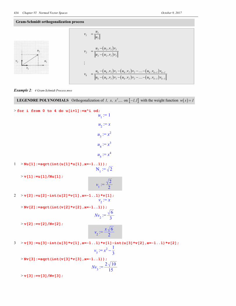
Gram-Schmidt orthogonalization process
1v 1
1
uu
=
2v ( )( )
2 2 1 1
2 2 1 1
u u ,v vu u ,v v
−=
−
kv ( ) ( ) ( )( ) ( ) ( )
k k 1 1 k 2 2 k k 1 k 1
k k 1 1 k 2 2 k k 1 k 1
u u ,v v u ,v v u ,v vu u ,v v u ,v v u ,v v
− −
− −
− − − −=
− − − −
Example 2: 4 Gram-Schmidt Process.mws LEGENDRE POLYNOMIALS Orthogonalization of 21, x, x ,... on [ ]1,1− with the weight function ( )w x 1= > for i from 0 to 4 do u[i+1]:=x^i od;
:= u1 1
:= u2 x
:= u3 x2
:= u4 x3
:= u5 x4
1 > Nu[1]:=sqrt(int(u[1]*u[1],x=-1..1)); := Ν1 2
> v[1]:=u[1]/Nu[1];
:= v12
2
2 > v[2]:=u[2]-int(u[2]*v[1],x=-1..1)*v[1]; := v2 x
> Nv[2]:=sqrt(int(v[2]*v[2],x=-1..1));
:= Nv263
> v[2]:=v[2]/Nv[2];
:= v2x 6
2
3 > v[3]:=u[3]-int(u[3]*v[1],x=-1..1)*v[1]-int(u[3]*v[2],x=-1..1)*v[2];
:= v3 − x2 13
> Nv[3]:=sqrt(int(v[3]*v[3],x=-1..1));
:= Nv32 10
15
> v[3]:=v[3]/Nv[3];
1u
2u
1v
2v

Chapter VI Normed Vector Spaces October 9, 2017
435
:= v3
3
− x2 1
3 10
4
Fourier coefficients > for n to 5 do c[n]:=evalf(int(f(x)*v[n],x=-1..1)) od; := c1 0.9802581433
:= c2 0.
:= c3 -0.179784401
:= c4 0. := c5 0.068153132
Fourier Series > fL(x):=sum(c[n]*v[n],n=1..5);
( )fL x 0.4901290716 2 0.1348383008
− x2 1
3 10 − :=
0.4472549288
+ − x4 3
3567 x2 2 +
TCHEBYSHEV'S POLYNOMIALS Orthogonalization of 21, x, x , ... on [ ]1,1− with a weights ( )2
1w x1 x
=−
The weight function: > w(x):=1/sqrt(1-x^2);
:= ( )w x 1 − 1 x2
1 > Nu[1]:=sqrt(int(u[1]*u[1]/sqrt(1-x^2),x=-1..1)); := Ν1 π
> v[1]:=u[1]/Nu[1];
:= v11π
2 > v[2]:=u[2]-int(u[2]*v[1]/sqrt(1-x^2),x=-1..1)*v[1]; := v2 x
> Nv[2]:=sqrt(int(v[2]*v[2]/sqrt(1-x^2),x=-1..1));
:= Nv22 π
2
> v[2]:=v[2]/Nv[2];
:= v2x 2
π
3 > v[3]:=u[3]-int(u[3]*v[1]/sqrt(1-x^2),x=-1..1)*v[1]-int(u[3]*v[2]/sqrt(1-x^2),x=-1..1)*v[2];
:= v3 − x2 12

Chapter VI Normed Vector Spaces October 9, 2017 436
> Nv[3]:=sqrt(int(v[3]*v[3]/sqrt(1-x^2),x=-1..1));
:= Nv32 π
4
> v[3]:=v[3]/Nv[3];
:= v3
2
− x2 1
2 2
π
Fourier Coefficients: > for n to 5 do a[n]:=int(f(x)*v[n]/sqrt(1-x^2),x=-1..1) od;
:= a12π
:= a2 0
:= a3 −2 2 ( )− + 3 π
π
:= a4 0
:= a5 −2 2 ( )− + 19 6 π
3 π
Fuorier’s Series: > fT(x):=sum(a[n]*v[n],n=1..5);
:= ( )fT x − −
2π
8 ( )− + 3 π
− x2 1
2π
32 ( )− + 19 6 π
+ − x4 1
8 x2
3 π
Tchebyshev :
Comparison of Legendre and Tchebyshev:

Chapter VI Normed Vector Spaces October 9, 2017
437
Lvov, Ukraine Stefan Banach
Lvov State University where Stefan Banach worked in 1919-1945
The Szkocka Café (Scottish Café) in Lvov, Ukraine Otto Nikodym and Stefan Banach
The café was a meeting place for many mathematicians including Banach, Steinhaus, Ulam, Mazur, Kac, Schauder, Kaczmarz and others. Problems were written in a book kept by the owner of the cafe and often prizes were offered for their solution. A collection of these problems appeared later in: R D Mauldin, The Scottish Book, Mathematics from the Scottish Café (1981) which contains the problems as well as some solutions and commentaries.

Chapter VI Normed Vector Spaces October 9, 2017 438
VI.3 EIGENVALUE PROBLEM Find the values of the parameter λ for which the operator equation
uLu λ= (4)
subject to boundary conditions has a non-trivial solution. Under some conditions, this eigenvalue problem will generate the required set of orthogonal functions. These conditions are formulated in the fundamental theorem as the regular Sturm-Liouville Theorem.
Sturm-Liouville Problem: For the homogeneous ordinary differential equation
( ) ( ) ( ) r x u q x p x u 0λ′′ + + = (5) subject to the homogeneous boundary conditions: ( ) ( ) 0xubxua 1111 =′− (6) ( ) ( )2 2 2 2a u x b u x 0′+ = (7) where 0b,b,a,a 2121 ≥ , and 0ba 11 >+ , 0ba 22 >+
( ) 0xp > , ( ) [ ]21 x,xCxp ∈ (8)
( ) 0xr > , ( ) [ ]211 x,xCxr ∈ (9)
( ) ( )21 x,xCxq ∈ (10)
find values of the parameter λ for which differential equation (5) subject to boundary conditions (6,7) has a non-trivial solution
( ) ( ) [ ]211
212 x,xCx,xCxu ∪∈ , ( ) ( )2
1 2u x L x ,x′′ ∈
1. Coefficients in the boundary conditions (6-7) are assumed to be non-negative 0b,b,a,a 2121 ≥ (that also means each pair of coefficients 1 1a ,b and 2 2a ,b cannot be equal to zero simultaneously.
2. Differential equation written in the form (5) with the coefficients satisfying the conditions (8-10) is said to be in Sturm-Liouville or self-adjoint form.
3. If both conditions (6) and (7) are held, then SLP is called regular. Sturm-Liouville Operator Consider the differential operator ( ) [ ]21
121
2 x,xCx,xC:L ∪ ( )21 2L x ,x→
written in self-adjoint form:
( )
+′′−≡ quur
p1Lu (12)
which rewrites the Sturm-Liouville problem (5) in the form
uLu λ= (13)
This is an eigenvalue problem for the differential operator L consisting in finding the values of parameter λ (eigenvalues) for which the operator equation (13) subject to boundary conditions (6-7) has non-trivial solutions (eigenfunctions).
Chapter VI Normed Vector Spaces October 9, 2017
439
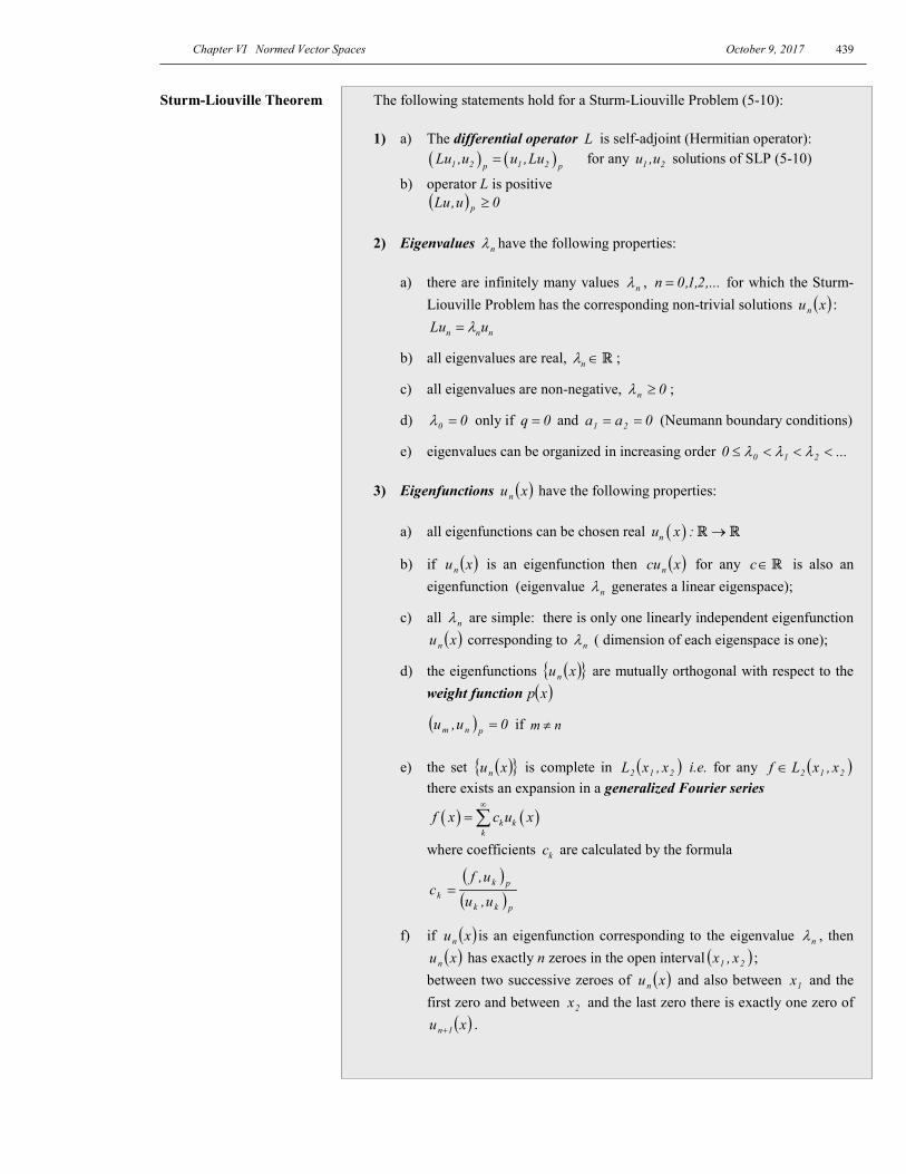
Sturm-Liouville Theorem The following statements hold for a Sturm-Liouville Problem (5-10): 1) a) The differential operator L is self-adjoint (Hermitian operator): ( ) ( )1 2 1 2p pLu ,u u ,Lu= for any 1 2u ,u solutions of SLP (5-10)
b) operator L is positive ( ) 0u,Lu p ≥ 2) Eigenvalues nλ have the following properties:
a) there are infinitely many values nλ , ,...2,1,0n = for which the Sturm-Liouville Problem has the corresponding non-trivial solutions ( )xun :
n n nLu uλ=
b) all eigenvalues are real, nλ ∈ ;
c) all eigenvalues are non-negative, 0n ≥λ ;
d) 00 =λ only if 0q = and 0aa 21 == (Neumann boundary conditions)
e) eigenvalues can be organized in increasing order ...0 210 <<<≤ λλλ 3) Eigenfunctions ( )xun have the following properties: a) all eigenfunctions can be chosen real ( )nu x : →
b) if ( )xun is an eigenfunction then ( )xcun for any c ∈ is also an eigenfunction (eigenvalue nλ generates a linear eigenspace);
c) all nλ are simple: there is only one linearly independent eigenfunction ( )xun corresponding to nλ ( dimension of each eigenspace is one);
d) the eigenfunctions ( ){ }xun are mutually orthogonal with respect to the weight function ( )xp
( ) 0u,u pnm = if nm ≠
e) the set ( ){ }xun is complete in ( )212 x,xL i.e. for any ( )212 x,xLf ∈ there exists an expansion in a generalized Fourier series
( ) ( )k kk
f x c u x∞
= ∑
where coefficients kc are calculated by the formula
( )( ) pkk
pkk u,u
u,fc =
f) if ( )xun is an eigenfunction corresponding to the eigenvalue nλ , then ( )xun has exactly n zeroes in the open interval ( )21 x,x ;
between two successive zeroes of ( )xun and also between 1x and the first zero and between 2x and the last zero there is exactly one zero of
( )xu 1n+ .
Chapter VI Normed Vector Spaces October 9, 2017 440
Reduction to self-adjoint form
If the linear differential equation with a parameter λ is given in standard form ( ) ( ) ( )0 1 2a x u a x u a x u 0λ′′ ′ + + + = then with the help of the multiplication factor
( )
( )( )
( )
1
0
a xdx
a x
0
exa x
µ =∫
(11)
it can be reduced to the self-adjoint form
( ) ( ) ( ) ( ) ( )0 2a x x u a x x x u 0µ µ λµ′′ + + =
The corresponding coefficients of equation (5) are identified as
( ) ( ) ( )( )( )
1
0
a xdx
a x0r x a x x e 0µ= = >
∫ , ( ) ( )
( )( )
( )
1
0
a xdx
a x
0
ep x x 0a x
µ= = >∫
if ( )0a x 0>
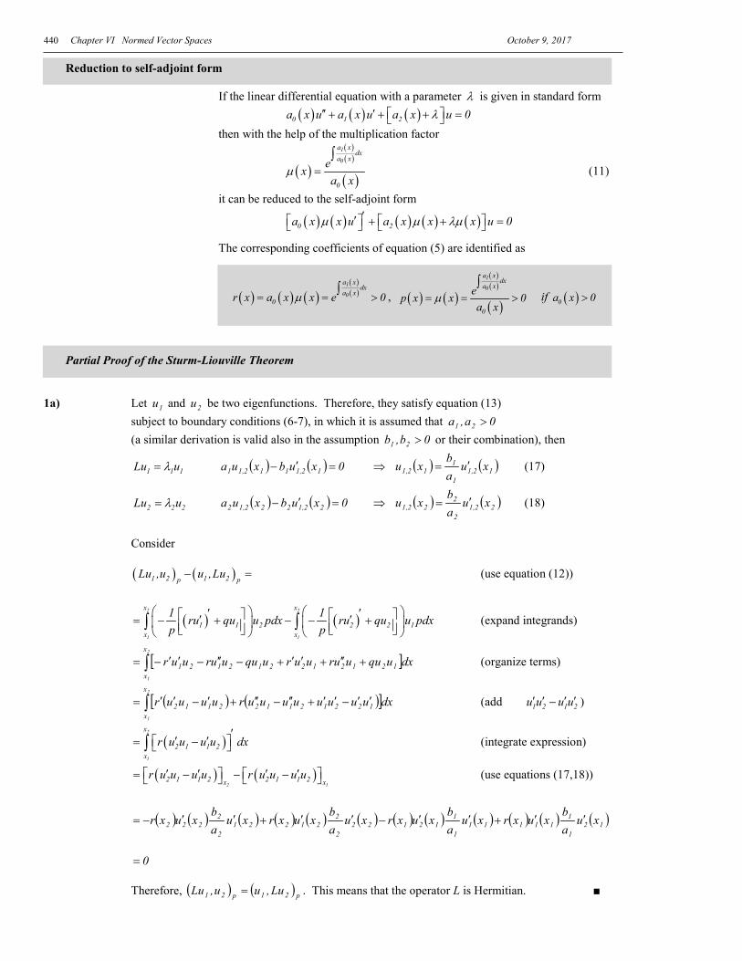
Partial Proof of the Sturm-Liouville Theorem
1a) Let 1u and 2u be two eigenfunctions. Therefore, they satisfy equation (13) subject to boundary conditions (6-7), in which it is assumed that 0a,a 21 >
(a similar derivation is valid also in the assumption 0b,b 21 > or their combination), then
1 1 1Lu uλ= ( ) ( ) 0xubxua 12,1112,11 =′− ⇒ ( ) ( )12,11
112,1 xu
ab
xu ′= (17)
2 2 2Lu uλ= ( ) ( ) 0xubxua 22,1222,12 =′− ⇒ ( ) ( )22,12
222,1 xu
ab
xu ′= (18)
Consider
( ) ( )1 2 1 2p pLu ,u u ,Lu− = (use equation (12))
( ) ( )2 2
1 1
x x
1 1 2 2 2 1x x
1 1ru qu u pdx ru qu u pdxp p
′ ′ ′ ′= − + − − + ∫ ∫ (expand integrands)
[ ]∫ +′′+′′+−′′−′′−=2
1
x
x121212212121 dxuquuuruuruquuuruur (organize terms)
( ) ( )[ ]∫ ′′−′′+′′−′′+′−′′=2
1
x
x122121122112 dxuuuuuuuuruuuur (add 1 2 1 2u u u u′ ′ ′ ′− )
( )2
1
x
2 1 1 2x
r u u u u dx′
′ ′ = − ∫ (integrate expression)
( ) ( )2 1
2 1 1 2 2 1 1 2x xr u u u u r u u u u′ ′ ′ ′ = − − − (use equations (17,18))
( ) ( ) ( ) ( ) ( ) ( ) ( ) ( ) ( ) ( ) ( ) ( )121
111111
1
112122
2
221221
2
2222 xu
ab
xuxrxuab
xuxrxuab
xuxrxuab
xuxr ′′+′′−′′+′′−=
0=
Therefore, ( ) ( ) p21p21 Lu,uu,Lu = . This means that the operator L is Hermitian. ■

Chapter VI Normed Vector Spaces October 9, 2017
441
1b) Operator L is positive
( ) ( ) ( ) 0dxxpxuu,Lu2
1
x
x
2npnn ≥= ∫ (from condition (9), ( ) 0xp > ) ■
2 b) Let nλ be an eigenvalue and nu be the corresponding eigenfunction, then
n n nLu uλ= . Because the operator L is Hermitian, ( ) ( ) pnnpnn Lu,uu,Lu = . Then
( ) ( ) ( ) ( ) ( ) ( ) pnnnpnnnpnnpnnpnnnpnnn u,uu,uLu,uu,Luu,uu,u λλλλλ =====
⇒ nn λλ = . Therefore, eigenvalue nλ is real, Rn ∈λ . ■ 2c) Let nλ be an eigenvalue and nu be the corresponding eigenfunction, then
n n nLu uλ= . Consider
( ) ( ) ( ) 2n n n n n n n n n np p p
Lu ,u u ,u u ,u uλ λ λ= = = . Then
( )
0u
u,Lu2
n
pnnn ≥=λ (because the operator L is positive (2b)) ■
3d) Let mu and nu be two eigenfunctions: m m mLu uλ= and n n nLu uλ= . Consider ( )pnmm u,uλ ( )pnmm u,uλ=
( )pnm u,Lu=
( )pnm Lu,u= (operator is Hermitian)
( )pnnm u,u λ=
( )pnmn u,uλ= (eigenvalues are real)
Therefore, ( )( ) 0u,u pnmnm =− λλ
If nm ≠ , then 0nm ≠− λλ and ( ) 0u,u pnm = Therefore, eigenfunctions mu and nu are orthogonal if nm ≠ . 3f) Illustration of this property with the eigenfunctions ( )3u x and ( )4u x obtained from the solution of equation (20) with Robin-Robin boundary conditions in the interval [ ]0,2

Chapter VI Normed Vector Spaces October 9, 2017 442
VI.4 SLP for equation X X 0µ′′ − =
Consider a boundary value problem which is important for solution of classical PDE’s in the Cartesian coordinate system:
( ) ( )X x X x 0µ′′ − = [ ]x 0,L∈ (20) ( ) ( )1 1k X 0 h X 0 0′− + = (21)
( ) ( )2 2 k X L h X L 0′ + = (22)
Depending on coefficients, boundary conditions (21-22) can be in one of the three classical types (Dirichlet, Neumann, or Robin). There are nine possible different combinations of boundary conditions which yield different solutions.
We can see that equation (20) can be written in the Sturm-Liouville form (5) which produces non-negative eigenvalues only if the separation constant µ is
assumed to be non-positive 2nµ λ= − :
[ ] 2X Xλ′′− = (23)
In this equation, we identify: r 1 0= > , q 0= , p 1 0= > . So, the weight function is
p 1= The general solution of this 2nd order homogeneous linear ODE with constant coefficients is given by
( ) 1 2X x c cos x c sin xλ λ= + (24)
The solution of Sturm-Liouville Problem will consist in finding non-trivial solutions which satisfy boundary conditions (21-22). Consider some particular cases of boundary conditions:
a) The case of Dirichlet-Dirichlet boundary conditions:
( )X 0 0= Dirichlet (25)
( )X L 0= Dirichlet (26)
Substitution of solution (24) into the first boundary condition (25) yields
( )X 0 = 1 2c cos 0 c sin 0 0λ λ+ =
1 2c 1 c 0 0⋅ + ⋅ = And from this, the first coefficient 1c 0= . Then general solution (24) reduces to
( ) 2X x c sin xλ= (27)
Substitute it into the second boundary condition (26)
( )X L = 2c sin L 0λ =
Chapter VI Normed Vector Spaces October 9, 2017
443
Because one coefficient in the solution (24) 1c is already assumed to be zero, for a non-trivial solution ( )X x , the second coefficient should not be equal to zero, 2c 0≠ . Therefore, the following equation should be satisfied
sin L 0λ = (28)
This equation has infinitely many solutions
L nλ π=
where n is any integer. But we have to restrict ourself only to positive values of n (because negative values with odd function (27) do not satisfy equation (23), and zero yields the trivial solution). Therefore, the values of parameter λ for which we have non-trivial solutions of BVP (23,25,26) are eigenvalues
nLπλ = n 1,2,3,...= (29)
Then corresponding to these values of parameter solutions are eigenfunctions
( )n nnX x sin x sin xLπλ= = n 1,2,3,...= (30)
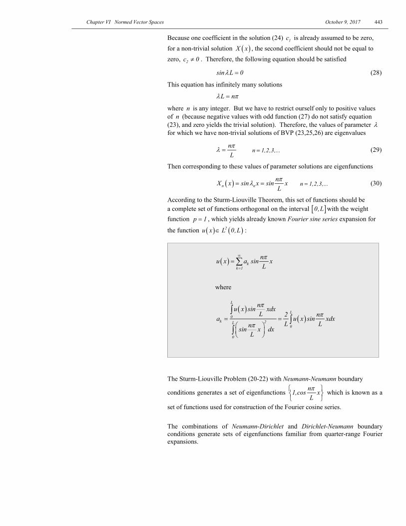
According to the Sturm-Liouville Theorem, this set of functions should be a complete set of functions orthogonal on the interval [ ]0,L with the weight function p 1= , which yields already known Fourier sine series expansion for
the function ( ) ( )2u x L 0,L∈ :
( ) kk 1
nu x a sin xLπ∞
=
= ∑
where
( )( )
L
L0
k 2L0
0
nu x sin xdxL 2 na u x sin xdx
L Lnsin x dxL
ππ
π= =
∫∫
∫
The Sturm-Liouville Problem (20-22) with Neumann-Neumann boundary
conditions generates a set of eigenfunctions n1,cos xLπ
which is known as a
set of functions used for construction of the Fourier cosine series.
The combinations of Neumann-Dirichlet and Dirichlet-Neumann boundary conditions generate sets of eigenfunctions familiar from quarter-range Fourier expansions.

Chapter VI Normed Vector Spaces October 9, 2017 444
b) The case of Robin-Dirichlet boundary conditions
( ) ( )1 1k X 0 h X 0 0′− + = Robin (denote 11
1
hHk
= ) (31)
( )X L 0= Dirichlet (32)
Application of the second boundary condition (32) first, eliminates one of the constants immediately, if the general solution (24) is rewritten in equivalent shifted form:
( ) ( ) ( )1 2X x c cos x L c sin x Lλ λ= − + − (24’)
Substitution of solution (24) into the second boundary condition (32) yields
( )X L = 1 2c cos 0 c sin 0 0λ λ+ =
1 2c 1 c 0 0⋅ + ⋅ =
from which yields that the first coefficient 1c 0= . Then the solution reduces to
( ) ( )2X x c sin x Lλ= −
Application of the Robin boundary condition requires also its derivative
( ) ( )2X x c cos x Lλ λ′ = −
Then at x 0=
( ) ( )1X 0 H X 0′− + ( ) ( )2 1c cos 0 L H sin 0 Lλ λ λ= − − + −
( )2 1c cos L H sin L 0λ λ λ= − − =
For the non-trivial solution 2c 0≠ , and, therefore
1cos L H sin L 0λ λ λ+ = (33)
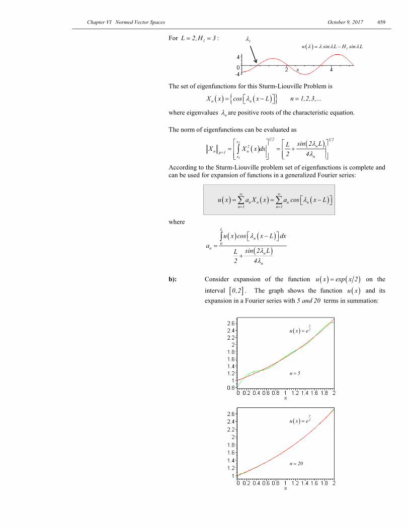
is a characteristic equation for eigenvalues nλ . There are infinitely many positive roots of this equation For example, for 1L 2,H 3= = :
Though 0 0λ = is a root of the characteristic equation, it is not an eigenvalue, because it produces a trivial solution.
The set of eigenfunctions for this Sturm-Liouville Problem is
( ) ( ){ }n nX x sin x Lλ= − n 1,2,3,...= (34)
where eigenvalues nλ are positive roots of the characteristic equation (33). The norm (3) of eigenfunctions can be evaluated as
( ) ( )2
1
1 2 1 2xn2
n np 1nx
sin 2 LLX X x dx2 4
λλ=
= = −
∫ (35)
According to the Sturm-Liouville problem set (34) is complete and can be used for expansion of functions in a generalized Fourier series (1):
1λ ( ) 1w cos L H sin Lλ λ λ λ= +

Chapter VI Normed Vector Spaces October 9, 2017
445
( ) ( ) ( )n n n nn 1 n 1
u x u X x u sin x Lλ∞ ∞
= =
= = −∑ ∑ (36)
where
( ) ( )
( )
L
n0
nn
n
u x sin x L dxu
sin 2 LL2 4
λ
λλ
−=
−
∫
Example: Consider expansion of the function ( ) ( )u x exp x 2= on the
interval [ ]0,2 . The graph shows the function ( )u x and its expansion in a Fourier series with 19 terms in summation:
With an increase of the number of terms (the next graph shows an approximation with 64 terms in the summation (36)), approximation by truncated Fourier series improves. There still is a presence of Gibb’s phenomena at the right boundary because eigenfunctions satisfying homogeneous Dirichlet boundary conditions are zero at x L= and there is a discontinuity with the non-zero value of the function ( )u x at this point.
( )x2u x e=
( )x2u x e=
n 19=
n 64=

Chapter VI Normed Vector Spaces October 9, 2017 446
c) The case of Dirichlet-Robin boundary conditions (solution with Maple) We will demonstrate how Maple can be used to generate the eigenvalues from
the characteristic equation and how the set of orthogonal functions is used for Generalized Fourier Series expansion of the function ( ) 4 xf x xe−= . Consider the following boundary value (Dirichlet-Robin):
X X 0µ′′ − = ( )x 0,L∈ ( )X 0 0= Dirichlet
( ) ( )2 2k X L h X L 0′ + = Robin 2
2
hHk
=
See Table 13 for Eigenvalues and Eigenfunctions of D-R SLP.
Maple example: > restart; > L:=1;H:=5;
:= L 1
:= H 5
Characteristic equation (Table 13 "sturm-liouville problem", case 5):
> w(x):=x*cos(x*L)+H*sin(x*L);
:= ( )w x + x ( )cos x 5 ( )sin x
> plot(w(x),x=0..12);
Eigenvalues:
> n:=1: for m from 1 to 30 do z:=fsolve(w(x)=0,x=m*2..(m+1)*2): if type(z,float) then lambda[n]:=z: n:=n+1 fi od: > for i to 5 do lambda[i] od;
2.653662400
5.454353755
8.391345550
11.40862652
14.46986802
> N:=n-1; := N 20
> n:='n':i:='i': Eigenfunctions:
> X[n]:=sin(lambda[n]*x); := Xn ( )sin λn x
Squared norm: > NX[n]:=int(X[n]^2,x=0..L);
:= NXn −12
− ( )cos λn ( )sin λn λn
λn

Chapter VI Normed Vector Spaces October 9, 2017
447
Function: > f(x):=x*exp(-4*x);
:= ( )f x x e( )−4 x
Fourier coefficients: > a[n]:=int(f(x)*X[n],x=0..L)/NX[n];
:= an
2 ( + + + − 24 e( )-4
λn ( )cos λn e( )-4
λn3
( )cos λn 80 e( )-4
( )sin λn 3 e( )-4
( )sin λn λn2
8 λn
( ) + 16 λn2
2
( ) − ( )cos λn ( )sin λn λn
Generalized Fourier series:
> u(x):=sum(a[n]*X[n],n=1..5): > plot({f(x),u(x)},x=0..L,axes=boxed);
> u(x):=sum(a[n]*X[n],n=1..N): > plot({f(x),u(x)},x=0..L,axes=boxed);
5 terms expansion
20 terms expansion

Chapter VI Normed Vector Spaces October 9, 2017 448
VI.5. TABLE SLP Results for all combinations of types of boundary conditions for Sturm-Liouville problems (20-22) are collected in the table Sturm-Liouville Problem. The table includes the kernel of integral transforms based on the corresponding boundary value problem, which also is used for solution of IBVP for PDE in the finite domains. Notice, that 0 0λ = is an eigenvalue only for the case of Neumann-Neumann boundary conditions when both coefficients 1 2h h 0= = (see 2d) of the Sturm-Liouville Theorem).
Chapter VI Normed Vector Spaces October 9, 2017
449
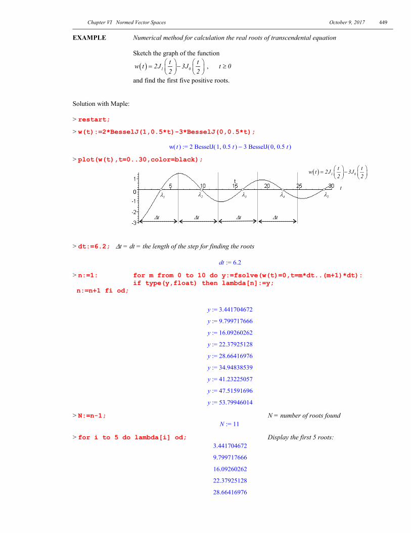
EXAMPLE Numerical method for calculation the real roots of transcendental equation Sketch the graph of the function
( ) 1 0t tw t 2J 3J2 2
= −
, t 0≥
and find the first five positive roots. Solution with Maple: > restart;
> w(t):=2*BesselJ(1,0.5*t)-3*BesselJ(0,0.5*t);
:= ( )w t − 2 ( )BesselJ ,1 0.5 t 3 ( )BesselJ ,0 0.5 t
> plot(w(t),t=0..30,color=black);
> dt:=6.2; t = dt = the length of the step for finding the roots∆
:= dt 6.2
> n:=1: for m from 0 to 10 do y:=fsolve(w(t)=0,t=m*dt..(m+1)*dt): if type(y,float) then lambda[n]:=y; n:=n+1 fi od;
:= y 3.441704672
:= y 9.799717666
:= y 16.09260262
:= y 22.37925128
:= y 28.66416976
:= y 34.94838539
:= y 41.23225057
:= y 47.51591696
:= y 53.79946014
> N:=n-1; N = number of roots found := N 11
> for i to 5 do lambda[i] od; Display the first 5 roots: 3.441704672
9.799717666
16.09260262
22.37925128
28.66416976
( ) 1 0t tw t 2J 3J2 2
= −
t
t∆ t∆ t∆ t∆
1λ 2λ 3λ 4λ 5λ
Chapter VI Normed Vector Spaces October 9, 2017 450
VI.6 REVIEW QUESTIONS 0) What is a vector space?
1) What is a norm in a vector space?
2) Give an example of normed vector space. 3) What is a metric vector space? 4) How can the metric be defined in a normed vector space? 6) Give an example of a metric space? 7) What is an inner product in a vector space? 8) How can the norm be defined in inner product space? 9) How is the convergence defined in a normed vector space? 10) What does it mean that normed vector space is complete? 11) What is Banach space? 12) What is Hilbert space? 13) Give examples of Banach and Hilbert spaces. 15) What are orthogonal vectors in inner product space? 16) What is an orthogonal set of vectors? 17) What is an orthonormal set?
18) How can the set of linear independent vectors be transformed to the orthonormal set?
19) What is vector space ( )2L a,b ? 20) How are inner product and weighted inner product defined in ( )2L a,b ? 21) What is the generalized Fourier series? 22) How are the coefficients in the generalized Fourier series calculated?
23) What does it mean that the set of functions in the vector space ( )2L a,b is complete? Give an example of the complete orthogonal set?
24) What is the eigenvalue problem for the operator equation? 25) Formulate the regular Sturm-Liouville Problem. 26) What are the properties of eigenvalues of the regular Sturm-Liouville
Problem? 27) What are the properties of eigenvectors of the regular Sturm-Liouville
Problem?

Chapter VI Normed Vector Spaces October 9, 2017
451
EXERCISES AND EXAMPLES 0. Prove that u v u v+ ≤ + for u,v ∈ .
1. Show that the set 1sin n x2 L
π +
is orthogonal in ( )2L 0,L .
2. a) Find eigenvalues and eigenfunctions of the following Sturm-Liouville
problem:
( ) ( ) X x X x 0µ′′ − =
( ) ( )X 0 HX 0 0′− + = Robin
( ) X L 0′ = Neumann
b) Use the obtained set of eigenfunctions for generalized Fourier series representation of the function
( ) xf x xe−= Sketch the graph for L 2= , H 3= , and n 5= and n 20= .
3. a) Find eigenvalues and eigenfunctions of the following Sturm-Liouville problem:
( ) ( )X x X x 0µ′′ − = ( ) ( )1X 0 H X 0 0′− + = Robin
( ) ( )2 X L H X L 0′ + = Robin (do not try to get the solution in the form given in the table for the Sturm-Liouville problem)
b) Use the obtained set of eigenfunctions for generalized Fourier series representation of the function
( ) xf x xe−= in the interval ( )0,L Sketch the graph for L 2= , H 3= , and n 5= and n 20= .
4. The steady state temperature distribution in the annular fin with variable cross-section is described by the differential equation (Incropera, p.139):
( )2
2
d T 1 dT 2h T T 0r dr ktdr ∞+ − − = 1 2L r L< <
Find the solution subject to boundary conditions: ( )1 1T L T=
( )2 2T L T= Sketch the graph of solution for:
1L 0.01 m= 2L 0.04 m= t 0.002 m=
Wk 150 m K
=⋅
2
Wh 250 m K
=⋅
o1T 500 C=
o2T 100 C=
oT 10 C∞ =

Chapter VI Normed Vector Spaces October 9, 2017 452
5. Prove that if the finite set { }k , k 1,2,...,nϕ = is orthonormal, then it is linearly independent. Solution:
Let 1 2 k n, ,..., ,...,ϕ ϕ ϕ ϕ be an orthonormal set. It means, that according to definition, the inner product
( )k m, 0ϕ ϕ = if k m≠
and ( )k k, 1ϕ ϕ = for all k ,m 1,2,...,n=
Assume that a linear combination of vectors from { }k , k 1,2,...,nϕ = is equal to zero:
1 1 2 2 3 k 4 nc c ... c ... c 0ϕ ϕ ϕ ϕ+ + + + + = Show that in this case all coefficients are equal to zero.
Calculate an arbitrary coefficient kc . For this, multiply both sides of equation by kϕ :
( ) ( )1 1 2 2 3 k 4 n k kc c ... c ... c , 0,ϕ ϕ ϕ ϕ ϕ ϕ+ + + + + = Use distributive property of inner product (p.396): ( ) ( ) ( ) ( )1 1 k 2 2 k k k k n n kc , c , ... c , ... c , 0ϕ ϕ ϕ ϕ ϕ ϕ ϕ ϕ+ + + + + =
Because vector kϕ is orthogonal to all other vectors, all terms in this equation except of one, are equal to zero:
k0 0 ... c 1 ... 0 0+ + + ⋅ + + = That means that coefficient kc 0=
Because it is an arbitrary coefficient, it means that all coefficients in the linear combination are equal to zero. Therefore, according to definition of linear independent set (p. 167), set { }k , k 1,2,...,nϕ = is linearly independent. q.e.d.

Chapter VI Normed Vector Spaces October 9, 2017
453
6. Show that the set 1sin n x2 L
π +
is orthogonal in ( )2L 0,L .
Solution:
Consider functions ( )n1x sin n x2 L
πϕ = + .
Function nϕ is orthogonal to function mϕ in space ( )2L 0,L , means that their inner product in this space defined by an integral (p.396) is zero:
( ) ( ) ( )L
n m n m0
, x x dx 0ϕ ϕ ϕ ϕ= =∫ when n m≠
Indeed,
( ) ( ) ( )L
n m n m0
, x x dxϕ ϕ ϕ ϕ= ∫
L
0
1 1sin n x sin m x dx2 L 2 L
π π = + + ∫
product to sum(p.43) L L
0 0
1 1 1 1cos n x m x dx cos n x m x dx2 L 2 L 2 L 2 L
π π π π = + − + − + + + ∫ ∫
( ) ( )L L
0 0
cos n m x dx cos n m 1 x dxL Lπ π = − − + + ∫ ∫
( ) ( )L L
0 0
sin n m x sin n m 1 xL Lπ π = − − + +
( ) ( )sin n m sin0 sin n m 1 sin0π π= − − − + + − n m , n m 1− ∈ + + ∈ =0 q.e.d.

Chapter VI Normed Vector Spaces October 9, 2017 454
TCHEBYSHEV'S POLYNOMIALS Orthogonalization of 21, x, x , ... on [ ]1,1− with a weights ( )2
1w x1 x
=−
7. The set { }2 31,x,x ,x ,... is linearly independent in ( )2L 1,1− .
a) Using the Gram-Schmidt orthogonalization algorithm with inner product
( ) ( ) ( )1
1
u,v u x v x dx−
= ∫
construct an orthonormal set in ( )2L 1,1− (the obtained set will be the set of the Legendre polynomials up to the scalar multiple).
b) Using the Gram-Schmidt orthogonalization algorithm with inner product
( ) ( ) ( )1
21
u x v xu,v dx
1 x−
=−
∫
construct an orthonormal set in ( )2L 1,1− (find just first 3 4− functions) (the obtained set will be the set of the Tchebyshev polynomials up the scalar multiple, see also Example 2).
c) Use the obtained orthonormal sets for generalized Fourier series expansion of the function:
( ) ( )( )
1 x 1,0f x
1 x 0,1− ∈ −= ∈
Compare the results for truncated series with 2,3,4 terms. Make some observations.

Chapter VI Normed Vector Spaces October 9, 2017
455
Solution: Follow Gram-Schmidt algorithm. Consider: ( )1u x 1= ( )2u x x= ( ) 2
3u x x= ( ) 3
4u x x= a)
( )1u x 1= 1 1
21 1
1 1
u u dx dx 2− −
= = =∫ ∫
11
1
u 2vu 2
= =
( ) ( )1
2 2 11
2u u ,v x x dx x2−
− = − =
∫
( ) ( )1
22 2 1 2 2 1
1
6u u ,v u u ,v dx3−
− = − = ∫
( )( )
2 2 1 12
2 2 1 1
u u ,v v 6v x2u u ,v v
−= =
−
( ) ( ) ( ) ( )1 1
2 2 2 23 3 2 2 3 1 1
1 1
6 2 1u u ,v v u ,v v x x x dx x dx x2 2 3− −
− − = − − = −
∫ ∫
( ) ( ) ( ) ( )1
23 3 2 2 3 1 1 3 3 2 2 3 1 1
1
2 10u u ,v v u ,v v u u ,v v u ,v v dx15−
− − = − − = ∫
( ) ( )( ) ( )
3 3 2 2 3 1 1 23
3 3 2 2 3 1 1
u u ,v v u ,v v 3 10 1v x4 3u u ,v v u ,v v
− − = = − − −
( ) ( ) ( ) 34 4 3 3 3 2 2 3 1 1
3u u ,v v u ,v v u ,v v x x5
− − − = −
( ) ( ) ( ) ( ) ( ) ( )1
24 4 3 3 3 2 2 3 1 1 4 4 3 3 3 2 2 3 1 1
1
2 14u u ,v v u ,v v u ,v v u u ,v v u ,v v u ,v v dx35−
− − − = − − − = ∫
( ) ( ) ( )( ) ( ) ( )
4 4 3 3 3 2 2 3 1 1 34
4 4 3 3 3 2 2 3 1 1
u u ,v v u ,v v u ,v v 5 14 3v x x4 5u u ,v v u ,v v u ,v v
− − − = = − − − −

Chapter VI Normed Vector Spaces October 9, 2017 456
b) ( )1u x 1= 21 11
1 2 21 1
u dxu dx1 x 1 x
π− −
= = =− −
∫ ∫
11
1
u 1vu π
= =
( ) ( )1
2 2 1 1 21
2 dxu u ,v v x x x2 1 x−
− = − = −
∫
( ) ( )1
22 2 1 1 2 2 1 2
1
dx 2u u ,v v u u ,v21 x
π
−
− = − = −
∫
( )( )
2 2 1 12
2 2 1 1
u u ,v v 2v xu u ,v v π
−= =
−
( ) ( ) 23 3 2 2 3 1 1
1u u ,v v u ,v v x2
− − = −
( ) ( ) ( ) ( )1
23 3 2 2 3 1 1 3 3 2 2 3 1 1 2
1
dx 2u u ,v v u ,v v u u ,v v u ,v v41 x
π
−
− − = − − = −
∫
( ) ( )( ) ( )
3 3 2 2 3 1 1 23
3 3 2 2 3 1 1
u u ,v v u ,v v 2 2 1v x2u u ,v v u ,v v π
− − = = − − −
( ) ( ) ( ) 34 4 3 3 3 2 2 3 1 1
3u u ,v v u ,v v u ,v v x x4
− − − = −
( ) ( ) ( )4 4 3 3 3 2 2 3 1 12u u ,v v u ,v v u ,v v8π
− − − =
( ) ( ) ( )( ) ( ) ( )
4 4 3 3 3 2 2 3 1 1 34
4 4 3 3 3 2 2 3 1 1
u u ,v v u ,v v u ,v v 4 2 3v x x4u u ,v v u ,v v u ,v v π
− − − = = − − − −
c) Generalized Fourier series ( ) ( )k kn
f x c v x= ∑ where Fourier coefficients are calculated by
( ) ( )1
k k1
c f x v x dx−
= ∫ for the case a)
( ) ( )1
k k 21
dxc f x v x1 x−
=−
∫ for the case b)
a: 12v
2= 2
6v x2
= 23
3 10 1v x4 3
= −
34
5 14 3v x x4 5
= −
4 25
105 2 6 3v x x16 7 35
= − +
b: 11vπ
= 22v xπ
= 23
2 2 1v x2π
= −
34
4 2 3v x x4π
= −
4 25
8 2 1v x x8π
= − +
T
case a) case b)
( )f x

Chapter VI Normed Vector Spaces October 9, 2017
457
Tchebyshev Functions Consider the Thebyschev equation (see RHB, p.596) ( )2 21 x y xy y 0ν′′ ′− − + = ν ∈ Any solution of the Tchebyshev equation is called a Tchebyshev function. Substitution x cosθ= 1cos xθ −=
d d1 cos sindx dx
θθ θ= = −
( )dy dy d 1 dyydx d dx sin d
θ θθ θ θ
′ = = = −
y′′ d 1 dydx sin dθ θ
= −
2
cos d dy 1 d dydx d sin d dxsin
θ θθ θ θθ
= − −
2
cos 1 dy dy 1 d 1 dysin d d sin d sin dsin
θθ θ θ θ θ θ θθ
= − − − −
2
3 2 2
cos dy dy 1 d yd dsin sin d
θθ θθ θ θ
= +
22
2
d y n y 0dθ
+ =
( ) ( )1 2y c cos n c sin nθ θ= + ( ) ( )y cos n i sin nθ θ= +
( ) ( ) ny cos i sinθ θ= +
( )n2y x i 1 x= + −
…………………

Chapter VI Normed Vector Spaces October 9, 2017 458
8. a) Find eigenvalues and eigenfunctions of the following Sturm-Liouville problem:
( ) ( )X x X x 0µ′′ − =
( ) ( )X 0 HX 0 0′− + = Robin
( ) X L 0′ = Neumann
b) Use the obtained set of eigenfunctions for generalized Fourier series representation of the function
( ) xf x xe−= Sketch the graph for L 2= , H 3= , and n 5= and n 20= . Solution: Follow Example b) on p.404. The Sturm-Liouville form of equation ( ) ( )X x X x 0µ′′ − = is
[ ] ( )X 0 X 0µ′′ + + − = where r 1 0, q 0, p 1 0= > = = > which implies that parameter 0µ− > (statement 1c of Sturm-Liouville
Theorem, p.401), therefore 0µ < . Denote 2 , 0µ λ λ= − > .
Then equation becomes
( ) ( )2X x X x 0λ′′ + =
Auxiliary equation 2 2m 0λ+ = , roots m iλ= ± . Because the second boundary condition is simpler and can be applied first, use the shifted form of solution:
( ) ( ) ( )1 2X x c cos x L c sin x Lλ λ = − + −
Differentiate: ( ) ( ) ( )1 2X x c sin x L c cos x Lλ λ λ λ′ = − − + − Substitution of solution into the second boundary condition yields
( )X L′ [ ] [ ]1 2c sin 0 c cos 0λ λ= − +
1 2c 0 c 1λ λ= ⋅ ⋅ + ⋅ ⋅
2c 0λ= ⋅ = ⇒ 2c 0= because 0λ >
Therefore, solution becomes
( ) ( )2X x c cos x Lλ = −
( ) ( )2X x c sin x Lλ λ′ = − −
Then application of boundary condition at x 0= yields:
( ) ( )1X 0 H X 0′− + ( ) ( )2 1 2c sin 0 L H c cos 0 Lλ λ λ = − + −
( ) ( )2 1 2c sin L H c cos Lλ λ λ= − +
For the non-trivial solution 2c 0≠ , and, therefore
( ) ( )1sin L H cos L 0λ λ λ− =
is a characteristic equation for eigenvalues nλ .
Chapter VI Normed Vector Spaces October 9, 2017
459
For 1L 2,H 3= = :
The set of eigenfunctions for this Sturm-Liouville Problem is
( ) ( ){ }n nX x cos x Lλ = − n 1,2,3,...=
where eigenvalues nλ are positive roots of the characteristic equation.
The norm of eigenfunctions can be evaluated as
( ) ( )2
1
1 2 1 2xn2
n np 1nx
sin 2 LLX X x dx2 4
λλ=
= = +
∫
According to the Sturm-Liouville problem set of eigenfunctions is complete and can be used for expansion of functions in a generalized Fourier series:
( ) ( ) ( )n n n nn 1 n 1
u x a X x a cos x Lλ∞ ∞
= =
= = − ∑ ∑
where
( ) ( )
( )
L
n0
nn
n
u x cos x L dxa
sin 2 LL2 4
λ
λλ
− =
+
∫
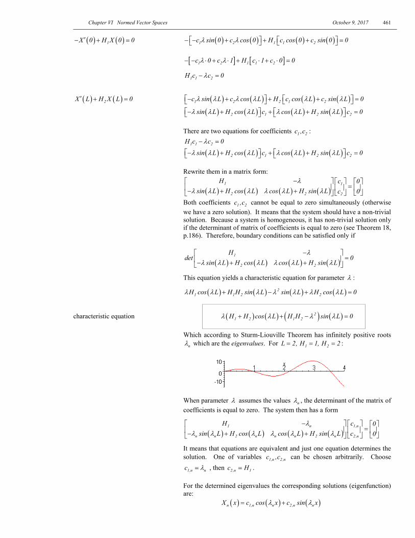
b): Consider expansion of the function ( ) ( )u x exp x 2= on the
interval [ ]0,2 . The graph shows the function ( )u x and its expansion in a Fourier series with 5 and 20 terms in summation:
( )x2u x e=
n 20=
( )x2u x e=
n 5=
1λ( ) 1w sin L H sin Lλ λ λ λ= −

Chapter VI Normed Vector Spaces October 9, 2017 460
9. a) Find eigenvalues and eigenfunctions of the following Sturm-Liouville problem:
( ) ( )X x X x 0µ′′ − = ( )X 0 0′ = Neumann
( ) ( )2X L H X L 0′ + = Robin
b) Use the obtained set of eigenfunctions for generalized Fourier series representation of the function
( ) xf x xe−=
Sketch the graph for L 2= , H 3= , and n 5= and n 20= .
10. a) Find eigenvalues and eigenfunctions of the following Sturm-Liouville problem:
( ) ( )X x X x 0µ′′ − = ( ) ( )1X 0 H X 0 0′− + = Robin
( ) ( )2X L H X L 0′ + = Robin (do not try to get the solution in the form given in the table for the Sturm-Liouville problem)
b) Use the obtained set of eigenfunctions for generalized Fourier series representation of the function
( ) xf x xe−= in the interval ( )0,L Sketch the graph for L 2= , H 3= , and n 5= and n 20= . Solution: Follow Example b) on p.404 and the previous problem #5. The Sturm-Liouville form (Eq.5, p.400) of equation ( ) ( )X x X x 0µ′′ − = is
[ ] ( )X 0 X 0µ′′ + + − = where r 1 0, q 0, p 1 0= > = = > which implies that parameter 0µ− > (statement 1c of Sturm-Liouville
Theorem, p.401), therefore 0µ < . Denote 2 , 0µ λ λ= − > .
Then equation becomes
( ) ( )2X x X x 0λ′′ + =
Auxiliary equation 2 2m 0λ+ = , roots m iλ= ± .
Because both boundary conditions are similar, use a non-shifted form of solution:
( ) ( ) ( )1 2X x c cos x c sin xλ λ= +
Differentiate:
( ) ( ) ( )1 2X x c sin x c cos xλ λ λ λ′ = − +
Substitution of solution into the boundary conditions yields
Chapter VI Normed Vector Spaces October 9, 2017
461
( ) ( )1X 0 H X 0 0′− + = ( ) ( ) ( ) ( )1 2 1 1 2c sin 0 c cos 0 H c cos 0 c sin 0 0λ λ − − + + + =
[ ] [ ]1 2 1 1 2c 0 c 1 H c 1 c 0 0λ λ− − ⋅ + ⋅ + ⋅ + ⋅ =
1 1 2H c c 0λ− =
( ) ( )2X L H X L 0′ + = ( ) ( ) ( ) ( )1 2 2 1 2c sin L c cos L H c cos L c sin L 0λ λ λ λ λ λ − + + + =
( ) ( ) ( ) ( )2 1 2 2sin L H cos L c cos L H sin L c 0λ λ λ λ λ λ − + + + = There are two equations for coefficients 1 2c ,c : 1 1 2H c c 0λ− =
( ) ( ) ( ) ( )2 1 2 2sin L H cos L c cos L H sin L c 0λ λ λ λ λ λ − + + + = Rewrite them in a matrix form:
( ) ( ) ( ) ( )1 1
2 2 2
H c 0sin L H cos L cos L H sin L c 0
λλ λ λ λ λ λ
− = − + +
Both coefficients 1 2c ,c cannot be equal to zero simultaneously (otherwise we have a zero solution). It means that the system should have a non-trivial solution. Because a system is homogeneous, it has non-trivial solution only if the determinant of matrix of coefficients is equal to zero (see Theorem 18, p.186). Therefore, boundary conditions can be satisfied only if
( ) ( ) ( ) ( )1
2 2
Hdet 0
sin L H cos L cos L H sin Lλ
λ λ λ λ λ λ−
= − + +
This equation yields a characteristic equation for parameter λ :
( ) ( ) ( ) ( )21 1 2 2H cos L H H sin L sin L H cos L 0λ λ λ λ λ λ λ+ − + =
characteristic equation ( ) ( ) ( ) ( )2
1 2 1 2H H cos L H H sin L 0λ λ λ λ+ + − =
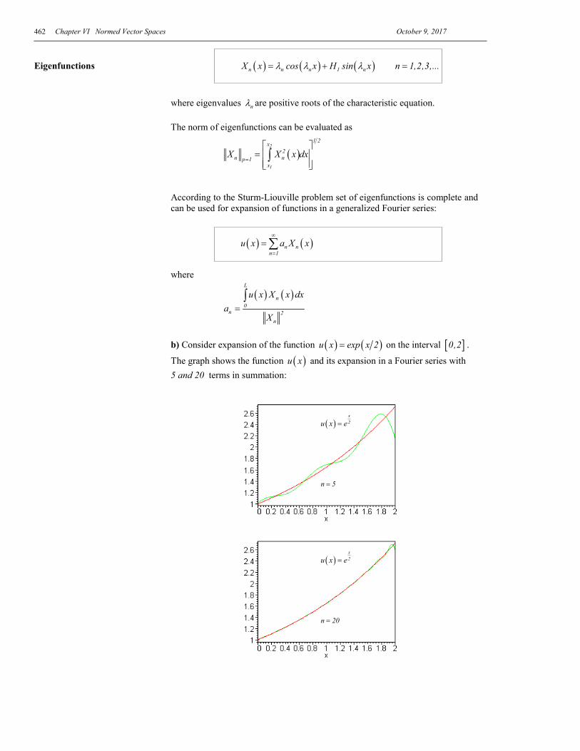
Which according to Sturm-Liouville Theorem has infinitely positive roots nλ which are the eigenvalues. For 1 2L 2, H 1, H 2= = = :
When parameter λ assumes the values nλ , the determinant of the matrix of coefficients is equal to zero. The system then has a form
( ) ( ) ( ) ( )1 n 1,n
n n 2 n n n 2 n 2,n
H c 0sin L H cos L cos L H sin L c 0
λλ λ λ λ λ λ
− = − + +
It means that equations are equivalent and just one equation determines the solution. One of variables 1,n 2,nc ,c can be chosen arbitrarily. Choose
1,n nc λ= , then 2,n 1c H= . For the determined eigenvalues the corresponding solutions (eigenfunction) are:
( ) ( ) ( )n 1,n n 2,n nX x c cos x c sin xλ λ= +
Chapter VI Normed Vector Spaces October 9, 2017 462
Eigenfunctions ( ) ( ) ( )n n n 1 nX x cos x H sin xλ λ λ= + n 1,2,3,...=
where eigenvalues nλ are positive roots of the characteristic equation.
The norm of eigenfunctions can be evaluated as
( )2
1
1 2x2
n np 1x
X X x dx=
=
∫
According to the Sturm-Liouville problem set of eigenfunctions is complete and can be used for expansion of functions in a generalized Fourier series:
( ) ( )n nn 1
u x a X x∞
=
= ∑
where
( ) ( )
L
n0
n 2n
u x X x dxa
X=
∫
b) Consider expansion of the function ( ) ( )u x exp x 2= on the interval [ ]0,2 .
The graph shows the function ( )u x and its expansion in a Fourier series with 5 and 20 terms in summation:
( )x2u x e=
n 5=
( )x2u x e=
n 20=
Chapter VI Normed Vector Spaces October 9, 2017
463
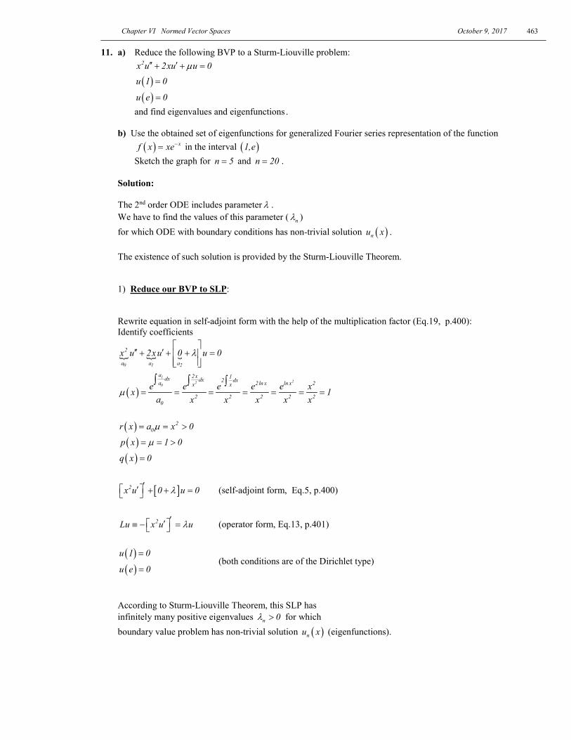
11. a) Reduce the following BVP to a Sturm-Liouville problem: 2x u 2xu u 0µ′′ ′+ + =
( )( )
u 1 0
u e 0
=
=
and find eigenvalues and eigenfunctions .
b) Use the obtained set of eigenfunctions for generalized Fourier series representation of the function ( ) xf x xe−= in the interval ( )1,e Sketch the graph for n 5= and n 20= .
Solution:
The 2nd order ODE includes parameter λ . We have to find the values of this parameter ( nλ ) for which ODE with boundary conditions has non-trivial solution ( )nu x .
The existence of such solution is provided by the Sturm-Liouville Theorem.
1) Reduce our BVP to SLP:
Rewrite equation in self-adjoint form with the help of the multiplication factor (Eq.19, p.400): Identify coefficients
0 1 2
2
a a ax u 2xu 0 u 0λ
′′ ′+ + + =
( )1
220
a 2 x 1dx dx 2 dxa 2ln x ln x 2x x
2 2 2 2 20
e e e e e xx 1a x x x x x
µ = = = = = = =∫ ∫ ∫
( ) 2
0r x a x 0µ= = >
( )p x 1 0µ= = >
( )q x 0=
[ ]2x u 0 u 0λ′ ′ + + = (self-adjoint form, Eq.5, p.400)
2Lu x u uλ′ ′≡ − = (operator form, Eq.13, p.401)
( )( )
u 1 0
u e 0
=
= (both conditions are of the Dirichlet type)
According to Sturm-Liouville Theorem, this SLP has infinitely many positive eigenvalues n 0λ > for which boundary value problem has non-trivial solution ( )nu x (eigenfunctions).
Chapter VI Normed Vector Spaces October 9, 2017 464
2) Find eigenvalues and eigenfunctions (solve BVP) 2x u 2xu u 0λ′′ ′+ + =
( )( )
u 1 0
u e 0
=
=
2nd order ODE, homogeneous, with variable coefficients, linear, Euler-Cauchy type
Auxiliary equation (see Table “linear o.d.e.” Euler-Cauchy Equation):
0 1 2
2
a a a1 x u 2 xu u 0λ′′ ′⋅ + + =
( )2
0 1 0 2a m a a m a 0+ − + =
( )2m 2 1 m 0λ+ − + = 2m m 0λ+ + =
1,21 1 4 1 1m
2 2 4λ λ− ± −
= = − ± −
case 1 1 04
λ− > 1 2m m≠ ⇒ 104
λ< <
general solution 1 2m m
1 2u c x c x= +
apply boundary conditions:
x 1= 1 20 c c= +
x e= 1 2m m1 20 c e c e= +
Rewrite as a system in matrix form:
1 2
1m m
2
c1 1 0ce e 0
=
2 1
1 2
m mm m
1 1det e e 0
e e
= − ≠
because 1 2m m≠
Therefore, system has only the trivial solution
1
2
c 0c 0
=
which yields the trivial solution of BVP.
Therefore, there is no eigenvalues in the interval
104
λ< <

Chapter VI Normed Vector Spaces October 9, 2017
465
case 2 1 04
λ− = 1 21m m2
= = −
general solution 1 12 2
1 2u c x c x ln x− −
= +
apply boundary conditions:
x 1= 1 20 c c 0= + ⋅ ⇒ 1c 0=
x e= 12
20 c e−
= ⇒ 2c 0=
It also yields the trivial solution.
case 3 1 04
λ− < ⇒ 14
λ >
( )1,21 1 1 1m 1 i2 4 2 4
λ λ = − ± − − = − ± −
general solution 12
1 21 1u c cos ln x c sin ln x x4 4
λ λ−
= − + −
apply boundary conditions:
x 1= 1 20 c cos0 c sin0= + ⇒ 1c 0=
12
21u c x sin ln x4
λ−
= −
x e= 1 12 2
2 21 10 c e sin ln e c e sin4 4
λ λ− −
= − = −
non-trivial solution only if
1sin 04
λ
− =
1 n4
λ π− = n 1,2,...=
2 21 n
4λ π− =
2 21 n4
λ π= + eigenvalues
( )n
sin n ln xu
xπ
= eigenfunctions

Chapter VI Normed Vector Spaces October 9, 2017 466
2nu
( ) 2e
1
sin n ln xdx
xπ
=
∫
( )2e
1
sin n ln xdx
xπ
= ∫
( ) [ ]e
2
1
1 sin n ln x d n ln xn
π ππ
= ∫
( ) ( ) e
1
sin n ln x cos n ln x1 n ln xn 2 2
π πππ
= −
( ) ( ) ( ) ( )sin n lne cos n lne sin n ln1 cos n ln11 n lne n ln1
n 2 2 2 2π π π ππ π
π
= − − −
12
=
b) Generalized Fourier series expansion:
( ) ( )n nn 1
f x c u x∞
=
= ∑
( )( ) ( ) ( )
en
n nn n 1
f ,uc 2 f x u x dx
u ,u= = ∫
Maple example for ( ) xf x xe−= :
> f:=x*exp(-x);
:= f x e( )−x
> u[n]:=sin(n*Pi*ln(x))/sqrt(x);
:= un( )sin n π ( )ln x
x
> N2[n]:=int(u[n]^2,x=1..exp(1));
:= N2n12
− + ( )cos n π ( )sin n π n πn π
> c[n]:=int(f*u[n],x=1..exp(1));
:= cn d⌠⌡
1
e
x e( )−x
( )sin n π ( )ln x x
> f5:=sum(c[n]*u[n]/N2[n],n=1..5): > f20:=sum(c[n]*u[n]/N2[n],n=1..20): > plot({f,f5,f20},x=1..exp(1));
n 5=n 20=
( ) xf x xe−=

Chapter VI Normed Vector Spaces October 9, 2017
467
12. a) Reduce the following BVP to a Sturm-Liouville problem: 2x u 3xu u 0µ′′ ′+ + =
( )( )
u 1 0
u e 0
=
′ =
and find eigenvalues and eigenfunctions .
b) Use the obtained set of eigenfunctions for generalized Fourier series representation of the function ( ) xf x xe−= in the interval ( )1, e
Sketch the graph for n 5= and n 20= . 13. a) Reduce the following BVP to a Sturm-Liouville problem:
xu u u 0xµ′′ ′+ + =
( )( )
u 1 0
u e 0
=
=
and find eigenvalues and eigenfunctions .
b) Use the obtained set of eigenfunctions for generalized Fourier series representation of the function ( ) xf x xe−= in the interval ( )1,e Sketch the graph for n 5= and n 20= .

Chapter VI Normed Vector Spaces October 9, 2017 468
14. Hermite’s differential equation with parameter λ is y 2xy y 0λ′′ ′− + = ( )x ,∈ −∞ ∞ , λ ∈ (HE)
a) Solve the Hermite Equation by the power series method b) Consider two linearly independent solutions
( )1y x ...=
( )2y x ...= which include parameter λ
c) If λ is a non-negative even integer, 0,2,4,...,2n,...λ = , then the series terminates, and one obtains, alternating for 1y and 2y , polynomials of degree n , which are multiples of so called Hermitian polynomials ( )nH x .
d) Rewrite HE in self-adjoint form and determine the weight function ( )w x
e) Check if the HP are orthogonal with the weight function ( )w x over ( ),−∞ ∞ :
( ) ( ) ( )m nH x H x w x dx 0∞
−∞
=∫ if m n≠
f) Give an example of function representation into Fourier-Hermite series
Solution: a) All points are ordinary points. We will apply a power-series solution method around the ordinary point 0x 0= (the interval of convergence for this solution is ( ),−∞ ∞ ). Assume that the solution is represented by a power series
∑∞
=
=0k
kk xay
then derivatives of the solution are
∑∞
=
−=′1k
1kk xkay
( )∑∞
=
−−=′′2k
2kk xa1kky
Substitute them into equation
( ) k 2 k 1 kk k k
k 2 k 1 k 0k k 1 a x 2x ka x a x 0λ
∞ ∞ ∞− −
= = =
− − + =∑ ∑ ∑
( ) ( )k 2 k kk k k
k 2 k 1 k 0k k 1 a x 2 ka x a x 0λ
∞ ∞ ∞−
= = =
− + − + =∑ ∑ ∑
Change of index: m k 2= − m k= m k= k m 2= +
( )( ) ( )m m mm 2 m m
m 0 m 1 m 0m 2 m 1 a x 2 ma x a x 0λ
∞ ∞ ∞
+= = =
+ + + − + =∑ ∑ ∑
( )Charles Hermite 1822 1901−
Chapter VI Normed Vector Spaces October 9, 2017
469
( )( ) ( )m 0
m m m2 0 m 2 m m
m 1 m 1 m 12 1 a a m 2 m 1 a x 2 ma x a x 0λ λ
=∞ ∞ ∞
+= = =
⋅ ⋅ + ⋅ + + + + − + =∑ ∑ ∑
( )( ) ( ) m2 0 m 2 m
m 12 1 a a m 2 m 1 a 2m a x 0λ λ
∞
+=
⋅ ⋅ + ⋅ + + + + − = ∑
Use identity Theorem (Theorem 2.6, Chapter 2):
02
aa
2 1λ ⋅
= −⋅
( )( )( )m 2 m
2ma a
m 2 m 1λ
+
−=
+ + m 1,2,...=
Write coefficients:
0a arbitrary=
1a arbitrary=
02
aa
2 1λ ⋅
= −⋅
( )3 1
2a a
3 2λ−
=⋅
( ) ( )4 2 0
2 2 2 2a a a
4 3 4 3 2 1λ λ λ⋅ − − ⋅ −
= =⋅ ⋅ ⋅ ⋅
( ) ( )( )5 3 1
2 3 2 3 2a a a
5 4 5 4 3 2λ λ λ⋅ − ⋅ − −
= =⋅ ⋅ ⋅ ⋅
( ) ( )( )6 4 0
2 4 2 4 2 2a a a
6 5 6 !λ λ λ λ⋅ − − ⋅ − ⋅ −
= =⋅
( ) ( )( )( )7 5 1
2 5 2 5 2 3 2 1a a a
7 6 7 !λ λ λ λ⋅ − ⋅ − ⋅ − ⋅ −
= =⋅
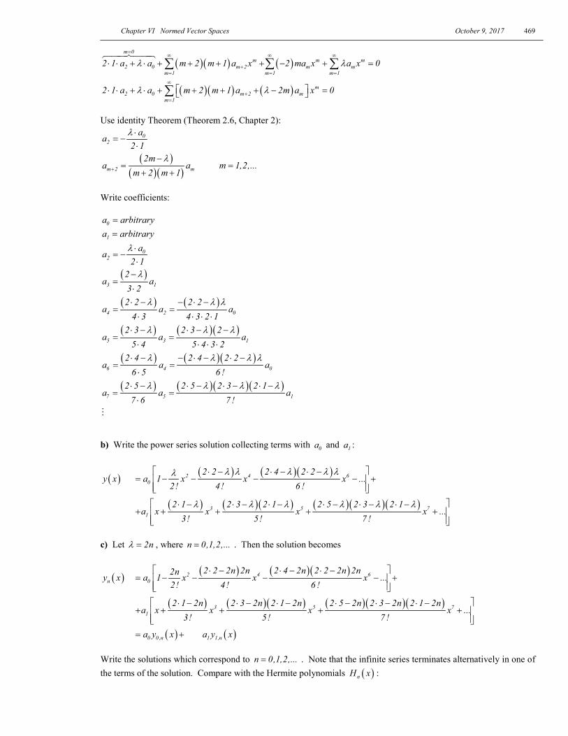
b) Write the power series solution collecting terms with 0a and 1a :
( )y x ( ) ( )( )2 4 6
0
2 2 2 4 2 2a 1 x x x ...
2! 4! 6 !λ λ λ λ λλ ⋅ − ⋅ − ⋅ −
= − − − − +
( ) ( )( ) ( )( )( )3 5 7
1
2 1 2 3 2 1 2 5 2 3 2 1a x x x x ...
3! 5! 7 !λ λ λ λ λ λ ⋅ − ⋅ − ⋅ − ⋅ − ⋅ − ⋅ −
+ + + + +
c) Let 2nλ = , where n 0,1,2,...= . Then the solution becomes
( )ny x ( ) ( )( )2 4 6
0
2 2 2n 2n 2 4 2n 2 2 2n 2n2na 1 x x x ...2! 4! 6 !
⋅ − ⋅ − ⋅ −= − − − − +
( ) ( )( ) ( )( )( )3 5 7
1
2 1 2n 2 3 2n 2 1 2n 2 5 2n 2 3 2n 2 1 2na x x x x ...
3! 5! 7 ! ⋅ − ⋅ − ⋅ − ⋅ − ⋅ − ⋅ −
+ + + + +
( )0 0 ,na y x= + ( )1 1,na y x Write the solutions which correspond to n 0,1,2,...= . Note that the infinite series terminates alternatively in one of the terms of the solution. Compare with the Hermite polynomials ( )nH x :
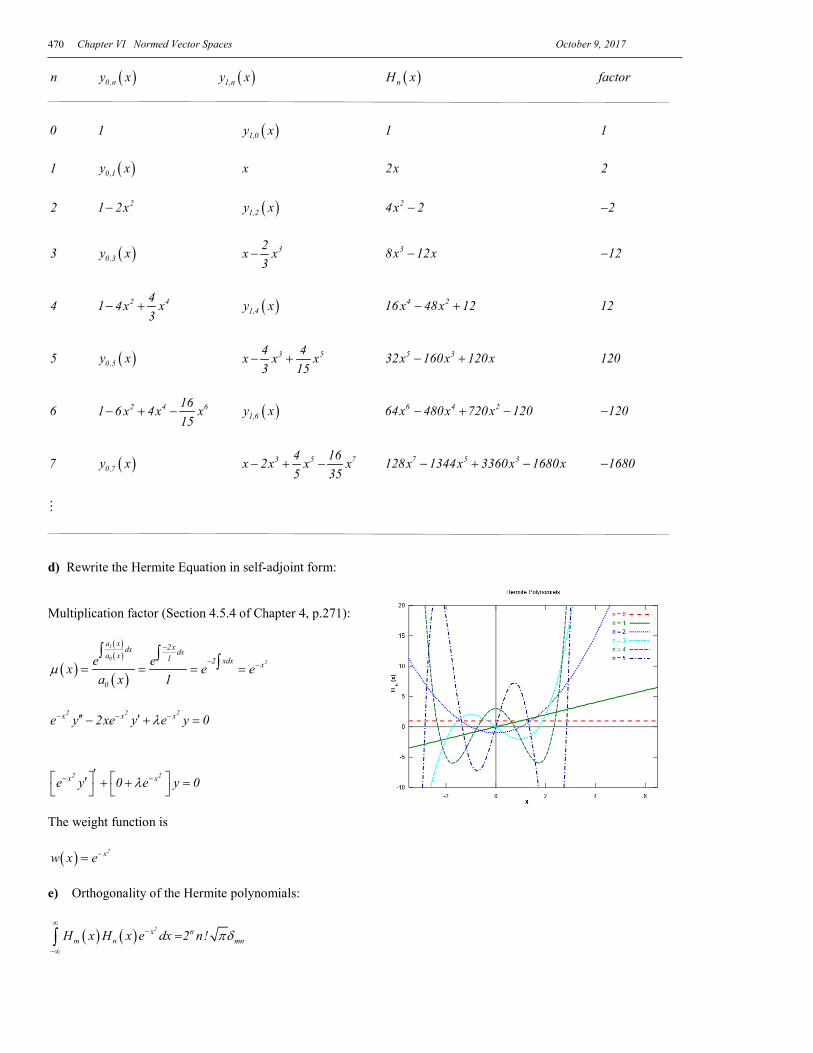
Chapter VI Normed Vector Spaces October 9, 2017 470
n ( )0 ,ny x ( )1,ny x ( )nH x factor 0 1 ( )1,0y x 1 1 1 ( )0 ,1y x x 2x 2 2 21 2x− ( )1,2y x 24x 2− 2−
3 ( )0 ,3y x 32x x3
− 38x 12x− 12−
4 2 441 4x x3
− + ( )1,4y x 4 216 x 48x 12− + 12
5 ( )0 ,5y x 3 54 4x x x3 15
− + 5 332x 160x 120x− + 120
6 2 4 6161 6 x 4x x15
− + − ( )1,6y x 6 4 264x 480x 720x 120− + − 120−
7 ( )0 ,7y x 3 5 74 16x 2x x x5 35
− + − 7 5 3128x 1344x 3360x 1680x− + − 1680−
d) Rewrite the Hermite Equation in self-adjoint form: Multiplication factor (Section 4.5.4 of Chapter 4, p.271):
( )
( )( )
( )
1
02
a x 2 xdx dxa x 1 2 xdx x
0
e ex e ea x 1
µ
−
− −= = = =∫ ∫ ∫
2 2 2x x xe y 2xe y e y 0λ− − −′′ ′− + =
2 2x xe y 0 e y 0λ− −′ ′ + + =
The weight function is
( ) 2xw x e−= e) Orthogonality of the Hermite polynomials:
( ) ( ) 2x nm n mnH x H x e dx 2 n! πδ
∞−
−∞
=∫
Chapter VI Normed Vector Spaces October 9, 2017
471
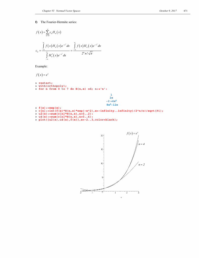
f) The Fourier-Hermite series:
( ) ( )n nn 0
f x c H x∞
=
= ∑
( ) ( )
( )
( ) ( )2 2
2
x xn n
n n2 xn
f x H x e dx f x H x e dxc
2 n!H x e dx π
∞ ∞− −
−∞ −∞∞
−
−∞
= =∫ ∫
∫
Example:
( ) xf x e= > restart; > with(orthopoly); > for n from 0 to 7 do H(n,x) od; n:='n':
1 2x
−2 +4x2
8x3−12x > f(x):=exp(x); > c[n]:=int(f(x)*H(n,x)*exp(-x^2),x=-infinity..infinity)/2^n/n!/sqrt(Pi); > u2(x):=sum(c[n]*H(n,x),n=0..2): > u4(x):=sum(c[n]*H(n,x),n=0..4): > plot({u2(x),u4(x),f(x)},x=-2..3,color=black);
( ) xf x e=
n 4=
n 2=

Chapter VI Normed Vector Spaces October 9, 2017 472

Chapter VI Normed Vector Spaces October 9, 2017
473
VI.7 More on normed vector spaces – theory and examples
Field of real numbers Define 2 u if u 0u u
u if u 0≥
= = − <. So, 2 2u u=
Prove that u v u v+ ≤ + for u,v ∈ .
Normed space Consider the space of real numbers with a norm defined as
x x=
Prove x y x y+ ≤ + for x, y ∈ .
Indeed, x y u v u v x y+ = + ≤ + = + ■
Metric space and a metric defines as
( )x, y x y x yρ = − = −
Prove ( ) ( ) ( )x, y x,z x,zρ ρ ρ≤ + for x, y,z ∈ .
Consider ( ) 2x, yρ ( )2 x y= −
( )2 x z z y= − + −
( ) ( ) ( )( )2 2 x z + z y 2 x z z y= − − + − −
2 2 x z + z y 2 x z z y≤ − − + − −
( )2 x z + z y≤ − −
( ) ( ) 2 x,z + z, yρ ρ≤
Therefore, ( )x, yρ ( ) ( ) x,z + z, yρ ρ≤ ■
Question: Define metric in as ( ) 1 if x y
x, y 0 if x y
ρ≠
= =.
That means that the distance between any two distinct points is unity. Is it a metric space?
Metric space n (Euclidian space) with a metric defined as
( ) ( )1 2n
2i i
i 1x, y x yρ
=
= − ∑
Metric space 0
n with a metric defined as
( ) i ii 1,2 ,..,nx, y max x yρ
== −
( )x, yρ ( )z, yρ
( )x,zρ
xy
z
x
yz
( )x, yρ
( )z, yρ
( )x,zρ
n

Chapter VI Normed Vector Spaces October 9, 2017 474
Normed space [ ]C a,b∞ Define [ ]( )C a,b , ∞
⋅ as a set of all continuous on [ ]a,b functions with
a norm ( )[ ]
( )x a ,b
f x max f x∞ ∈
= (maximum norm) .
Theorem [ ]C a,b∞ = [ ]( )C a,b , ∞
⋅ is a Banach space. That means that it has be shown that defined norm satisfies the norm axioms, and that the space [ ]C a,b∞ is complete with respect to convergence in defined norm.
1. Prove that ( )
[ ]( )
x a ,bf x max f x
∞ ∈= is a norm.
There always exists [ ]
( )x a ,bmax f x∈
because continuous on closed interval
Function attains its extreme values in [ ]a,b .
Prove that triangle inequality holds for the defined norm.
For absolute value, u v u v+ ≤ + . Then for any [ ]u,v C a,b∞∈
( )u v max u v max u v max u max v u v∞ ∞ ∞
+ = + ≤ + = + = + ■ 2. Prove completeness of the space [ ]C a,b∞ .
Let ( )kf x be a Cauchy sequence in [ ]C a,b∞ .
That means that n mf f 0− → when n,m → ∞ .
That means that for any 0ε > there exists a natural number N ∈ such that n mf f ε− < whenever both n N> and m N> .
According to definition of the norm
[ ]( ) ( ) ( ) ( )n m n m n mx a ,b
f f max f x f x f x f x∞ ∈
− = − ≥ − for all [ ]x a,b∈
therefore, ( ) ( )n mf x f x 0− → when n,m → ∞ .
That means that ( )kf x is a Cauchy sequence in the field of real numbers
for any fixed [ ]x a,b∈ .
Since the field of real numbers is complete, there exists a real number ( )f x ∈ such that ( ) ( )kf x f x→ .
Show that defined this way as a limit of a Cauchy sequence ( )kf x , is a
continuous function of x in [ ]a,b . That will mean that ( ) [ ]f x C a,b∞∈
and it will conclude the proof that ( ) ( )kf x f x→ in [ ]C a,b∞ .

Chapter VI Normed Vector Spaces October 9, 2017
475
Because of ( ) ( )n mf x f x 0− → when n,m → ∞ , as it is already said, for
any 0ε > there exists a natural number N ∈ such that n mf f ε− < when n N> and m N> .
Fix some n N> , and let m → ∞ . That yields, that ( ) ( )mf x f x→ .
Therefore, ( ) ( )nf x f x ε− < , and therefore, ( ) ( )nf x f x→ .
Fix the arbitrary [ ]0x a,b∈ and 0ε > .
Choose 0δ > such that ( ) ( )N N 0f x f x ε− < whenever 0x x δ− < .
Then whenever 0x x δ− < ,
( ) ( ) ( ) ( ) ( ) ( ) ( ) ( )0 N 0 N N 0 N 0 0f x f x f x f x f x f x f x f x 3ε− ≤ − + − + − <
.
Therefore, ( )f x is continuous at any [ ]0x a,b∈ , and therefore
( ) [ ]f x C a,b∞∈ and that ( ) ( )kf x f x→ in [ ]C a,b∞ .
Therefore, [ ]C a,b∞ is complete. ■
Vector Space ( )2L a,b The set of all functions ( )xϕ defined on the interval ( )a,b such that their
square ( )2 xϕ is an integrable function over ( )a,b :
( ) ( ) ( ) = → < ∞
∫
b2 2
a
L a,b : a,b such that x dxϕ ϕ
For ( )2u,v L a,b∈ define the inner product:
( ) ( ) ( )b
a
u,v u x v x dx= ∫ inner product in ( )2L a,b
( ) ( ) ( ) ( )b
pa
u,v u x v x p x dx= ∫ weighted inner product in ( )2L a,b
with the weight function ( )p x 0> Defined inner products induce the norms in ( )2L a,b :
( )1 2b
2
a
u u x dx
= ∫
( ) ( )1 2b
2p
a
u u x p x dx
= ∫ weighted norm
Theorem (Riesz-Fischer) The normed space ( )2L a,b is a Banach space.
Chapter VI Normed Vector Spaces October 9, 2017 476
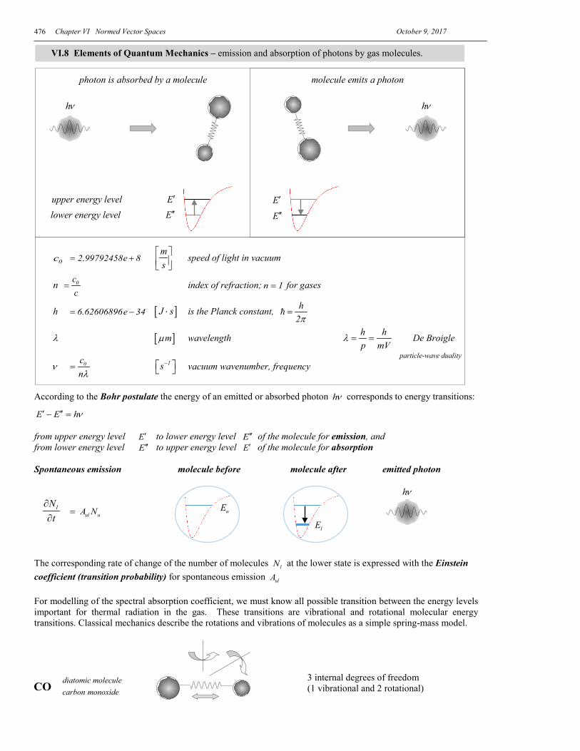
VI.8 Elements of Quantum Mechanics – emission and absorption of photons by gas molecules.
0c 2.99792458e 8= + ms
speed of light in vacuum
n 0cc
= index of refraction; n 1= for gases
h 6.62606896e 34= − [ ]J s⋅ is the Planck constant, h2π
=
λ [ ]mµ wavelength h hp mV
λ = = De Broigle
ν 0cnλ
= 1s− vacuum wavenumber, frequency
According to the Bohr postulate the energy of an emitted or absorbed photon hν corresponds to energy transitions:
E E hν′ ′′− = from upper energy level E′ to lower energy level E′′ of the molecule for emission, and from lower energy level E′′ to upper energy level E′ of the molecule for absorption Spontaneous emission molecule before molecule after emitted photon
lNt
∂∂
ul u A N=
The corresponding rate of change of the number of molecules lN at the lower state is expressed with the Einstein coefficient (transition probability) for spontaneous emission ulA For modelling of the spectral absorption coefficient, we must know all possible transition between the energy levels important for thermal radiation in the gas. These transitions are vibrational and rotational molecular energy transitions. Classical mechanics describe the rotations and vibrations of molecules as a simple spring-mass model. 3 internal degrees of freedom (1 vibrational and 2 rotational)
hνhν
photon is absorbed by a molecule molecule emits a photon
E′
E′′
upper energy level E′
lower energy level E′′
hν
uE
lE
CO diatomic moleculecarbon monoxide
particle-wave duality

Chapter VI Normed Vector Spaces October 9, 2017
477
Quantum mechanical treatment of the interaction of radiation with gaseous matter is based on the Schrödinger equation, which describes energy levels of molecules in contrast to classical electromagnetic treatment of radiation. The Schrödinger equation is the fundamental postulate of quantum mechanics; it describes the wave function corresponding to translation, vibration and rotation of molecules:
( ) ( ) ( ) ( )2
2
rV r r E r
2m rψ
ψ ψ∂
− + =∂
The equation above is the time-independent form of the Schrödinger equation describing the stationary states of molecules, where r is the intermolecular distance, ( )V r is the potential function, and E is the total energy. The
values of total energy jE for which the Schrödinger equation has non-zero solutions ( )i rψ are called eigenvalues,
and the corresponding functions ( )i rψ are called eigenfunctions. Quantum mechanical analysis yields that the molecule can rotate only with discrete rotational energy levels jE for which the Schrödinger equation has non-zero solutions. Example Deep potential well model (also can be treated as a motion of the particle in a one-dimensional box)
( ) ( )2
2
rE r
2m rψ
ψ∂
− =∂
( ) 0 0ψ =
( ) a 0ψ =
( ) ( )
2
2
2
r 2m E rr
µ
ψψ
∂= −
∂
naπµ =
2 2
2
2m nE aπ
=
⇒ 2 2
n 2
nE 2ma
π=
energy levels can be only of discrete values,
n is called a quantum number, n 1,2,...= Particle emits quants of discrete energy only:
( )2
22n n 1 2hν E E n n 1
2maπ
− = − = − −
( ) sinn2 n r ra a
πψ =
discrete wavefunctions
( ) sin2 2n
2 n r ra a
πψ =
probability distribution of particle’s position in box
r 0=
V 0=
rr a=
V = ∞V = ∞
V is a potential energy of the particle
particle can move along r-axisbetween walls r 0 and r a= =
Niels Bohr Erwin SchrodingerLouis de BroglieMax Planck Albert Einstein

Chapter VI Normed Vector Spaces October 9, 2017 478
www.tcheb.ru