chapter xiv: risk modeling - department of...
TRANSCRIPT
copyright 1997 Bruce A. McCarl and Thomas H. Spreen
1
CHAPTER XIV: RISK MODELING .................................................................................................... 2 14.1 Decision Making and Recourse ................................................................................................................ 3 14.2 An Aside: Discounting Coefficients ........................................................................................................ 4 14.3 Stochastic Programming without Recourse .......................................................................................... 4
14.3.1 Objective Function Coefficient Risk ................................................................................................ 4 14.3.1.1 Mean-Variance Analysis ................................................................................................................ 5
14.3.1.1.1 Example ..................................................................................................................................... 6 14.3.1.1.2 Markowitz's E-V Formulation ................................................................................................ 8 14.3.1.1.3 Formulation Choice ................................................................................................................. 8 14.3.1.1.4 Characteristics of E-V Model Optimal Solutions ................................................................ 8 14.3.1.1.5 E-V Model Use - Theoretical Concerns ................................................................................ 9 14.3.1.1.6 Specification of the Risk Aversion Parameter ................................................................... 10
14.3.1.2 A Linear Approximation - MOTAD ........................................................................................... 11 14.3.1.2.1 Example ................................................................................................................................... 13 14.3.1.2.2 Comments on MOTAD ......................................................................................................... 14
14.3.1.3 Toward A Unified Model ............................................................................................................. 16 14.3.1.4 Safety First...................................................................................................................................... 17
14.3.1.4.1 Example ................................................................................................................................... 18 14.3.1.4.2 Comments ................................................................................................................................ 18
14.3.1.5 Target MOTAD ............................................................................................................................. 18 14.3.1.5.1 Example ................................................................................................................................... 19 14.3.1.5.2 Comments ................................................................................................................................ 19
14.3.1.6 DEMP .............................................................................................................................................. 20 14.3.1.6.1 Example ................................................................................................................................... 21 14.3.1.6.2 Comments ................................................................................................................................ 21
14.3.1.7 Other Formulations ....................................................................................................................... 22 14.3.2 Right Hand Side Risk ........................................................................................................................ 22
14.3.2.1 Chance Constrained Programming ............................................................................................. 22 14.3.2.1.1 Example ................................................................................................................................... 24 14.3.2.1.2 Comments ................................................................................................................................ 24
14.3.2.2 A Quadratic Programming Approach ......................................................................................... 25 14.3.3 Technical Coefficient Risk ................................................................................................................ 26
14.3.3.1 Merrill's Approach ......................................................................................................................... 26 14.3.3.2 Wicks and Guise Approach .......................................................................................................... 27
14.3.3.2.1 Example ................................................................................................................................... 28 14.3.3.2.2 Comments ................................................................................................................................ 28
14.3.4 Multiple Sources of Risk ................................................................................................................... 29 14.4 Sequential Risk-Stochastic Programming with Recourse ................................................................ 29
14.4.1 Two stage SPR formulation ............................................................................................................. 29 14.4.1.1 Example .......................................................................................................................................... 32
14.4.2 Incorporating Risk Aversion ........................................................................................................... 33 14.4.2.1 Example .......................................................................................................................................... 34
14.4.3 Extending to Multiple Stages ........................................................................................................... 35 14.4.4 Model Discussion ................................................................................................................................ 37
14.5 General Comments On Modeling Uncertainty ................................................................................... 38 References ............................................................................................................................................................. 41

copyright 1997 Bruce A. McCarl and Thomas H. Spreen
2
CHAPTER XIV: RISK MODELING and Stochastic Programming
Risk is often cited as a factor which influences decisions. This chapter reviews methods for
incorporating risk and risk reactions into mathematical programming models.1
Stochastic mathematical programming models depict the risk inherent in model parameters and
possibly the decision maker’s response to that risk. Risk considerations are usually incorporated
assuming that the parameter probability distribution (i.e., the risk) is known with certainty.2 Usually, the
task becomes one of adequately representing these distributions as well as the decision makers response
to parameter risk.
The question arises: Why use stochastic models, why not just solve the model under all
combinations of the risky parameters and use the resultant plans? Such an approach is tempting, yet
suffers from problems of dimensionality and certainty. The dimensionality problem is manifest in the
number of possible solutions under the alternative settings for the uncertain parameters (i.e., five possible
values for each of three parameters would lead to 35 = 243 possible model specifications). Often, there
are more possible combinations of values of the risky parameters than can practically be enumerated.
Furthermore, these enumerated plans suffer from a certainty problem. Every LP parameter is assumed
known with perfect knowledge. Consequently, solutions reflect "certain" knowledge of the parameter
values imposed. Thus, when one solves many models one gets many plans and the question remains
which plan should be used.
Usually, it is desirable to formulate a stochastic model to generate a robust solution which yields
satisfactory results across the full distribution of parameter values. The risk modeling techniques
discussed below are designed to yield such a plan. The "optimal" plan for a stochastic model generally
does not place the decision maker in the best possible position for all (or maybe even any) possible
1 The risk modeling problem is a form of the multiple objective programming problem so that there
are parallels between the material here and that in the multi-objective chapter.
2 It should be noted that in this chapter risk and uncertainty are used interchangeably in a manner not consistent with some discussions in the literature where a distinction is made involving the degree to which a decision maker knows the parameter probability distributions(Knight). Any time we discuss risk or uncertainty we assume that the probability distribution is known.
copyright 1997 Bruce A. McCarl and Thomas H. Spreen
3
parameter combinations(commonly called states of nature or events), but rather establishes a robust
position across the set of possible events.
14.1 Decision Making and Recourse
Many different stochastic programming formulations have been posed for risk problems. An
important assumption involves the potential decision maker reaction to information. The most
fundamental distinction is between cases where:
1) all decisions must be made now with the uncertain outcomes resolved later, after all
random draws from the distribution have been taken, and 2) some decisions are made now, then later some uncertainties are resolved followed by
other decisions yet later.
These two settings are illustrated as follows. In the first case, all decisions are made then events
occur and outcomes are realized. This is akin to a situation where one invests now and then discovers the
returns to the investment at years end without any intermediate buying or selling decisions. In the second
case, one makes some decisions now, gets some information and makes subsequent decisions. Thus, one
might invest at the beginning of the year based on a year long consideration of returns, but could sell and
buy during the year depending on changes in stock prices.
The main distinction is that under the first situation decisions are made before any uncertainty is
resolved and no decisions are made after any of the uncertainty is resolved. In the second situation,
decisions are made sequentially with some decisions made conditional upon outcomes that were subject
to a probability distribution at the beginning of the time period.
These two frameworks lead to two very different types of risk programming models. The first
type of model is most common and is generally called a stochastic programming model without recourse.
The second type of model was originally developed by Dantzig in the early 50's and falls into the class of
stochastic programming with recourse models. These approaches are discussed separately, although
many of the “without recourse” techniques can be used when dealing with the “with recourse” problems.
copyright 1997 Bruce A. McCarl and Thomas H. Spreen
4
14.2 An Aside: Discounting Coefficients
Before discussing formal modeling approaches, first let us consider a common, simple approach
used in virtually all "risk free" linear programming studies. Suppose a parameter is distributed according
to some probability distribution, then a naive risk specification would simply use the mean. However,
one could also use conservative price estimates (i.e., a price that one feels will be exceeded 80% of the
time).
This reveals a common approach to risk. Namely, data for LP models are virtually never certain.
Conservative estimates are frequently used, in turn producing conservative plans (see McCarl et al., for an
example of treatment of time available). Objective function revenue and resource availability coefficients
may be deflated while cost coefficients are inflated. Technical coefficients and right hand sides may be
treated similarly. The main difficulty with a conservative estimate based approach is the resultant
probability of the solution. Conservative estimates for all parameters can imply an extremely unlikely
event (ie what is the chance that resource availability in every period will be at the low end of the
probability distribution at the same time as all prices) and cause the model to take on an overly
conservative choice of the decision variables.
14.3 Stochastic Programming without Recourse
Risk may arise in the objective function coefficients, technical coefficients or right hand sides
separately or collectively. Different modeling approaches have arisen with respect to each of these
possibilities and we will cover each separately.
14.3.1 Objective Function Coefficient Risk
Several objective function coefficient risk models have been posed. This section reviews these.
First, however, some statistical background on distributions of linear sums is necessary.
Given a linear objective function
where X1, X2 are decision variables and c1 , c2 are uncertain parameters distributed with means
and as well as variances s11 , s22, and covariance s12; then Z is distributed with mean
2211 XcXcZ
1c 2c

copyright 1997 Bruce A. McCarl and Thomas H. Spreen
5
and variance
In matrix terms the mean and variance of Z are
where in the two by two case
Defining terms sii is the variance of the objective function coefficient of Xi, which is calculated using the formula
sik = ∑ (cik- where cik is the kth observation on the objective value of Xi and N is the number of observations, assuming an equally likely probability (1/N) of occurrence.3
sij for i j is the covariance of the objective function coefficients between ci and cj, calculated by the
formula sij = ∑ (cik- )(cjk- )/N. Note sij = sji.
is the mean value of the objective function coefficient ci, calculated by ∑cik/N. (Assuming an equally likely probability of occurrence.)
14.3.1.1 Mean-Variance Analysis
The above expressions define the mean and variance of a LP objective function with risky c
parameters. Markowitz exploited this in the original mean-variance (or EV) portfolio choice formulation.
The portfolio choice problem involves development of an "optimal" investment strategy. The
variables indicate the amount of funds invested in each risky investment subject to a total funds
constraint. Markowitz motivated the formulation by observing that investors only place a portion, not all,
of their funds in the highest-yielding investment. This, he argued, indicated that a LP formulation is
inappropriate since such an LP would reflect investment of all funds in the highest yielding alternative
(since there is a single constraint). This divergence between observed and modeled behavior led
Markowitz to include a variance term resulting in the so-called expected value variance (EV) model.
3 One could also use the divisor N-1 when working with a sample.
2211 XcXcZ
.XXs2XsXs 21212222
2111
2Z
SX)X,XC(
.ss
ssSccC
2221
121121
/N)c 2i
ic jc
ic ic
copyright 1997 Bruce A. McCarl and Thomas H. Spreen
6
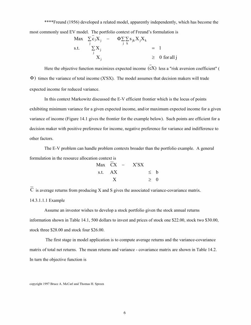
****Freund (1956) developed a related model, apparently independently, which has become the
most commonly used EV model. The portfolio context of Freund’s formulation is
Here the objective function maximizes expected income less a "risk aversion coefficient" (
times the variance of total income (X'SX). The model assumes that decision makers will trade
expected income for reduced variance.
In this context Markowitz discussed the E-V efficient frontier which is the locus of points
exhibiting minimum variance for a given expected income, and/or maximum expected income for a given
variance of income (Figure 14.1 gives the frontier for the example below). Such points are efficient for a
decision maker with positive preference for income, negative preference for variance and indifference to
other factors.
The E-V problem can handle problem contexts broader than the portfolio example. A general
formulation in the resource allocation context is
is average returns from producing X and S gives the associated variance-covariance matrix.
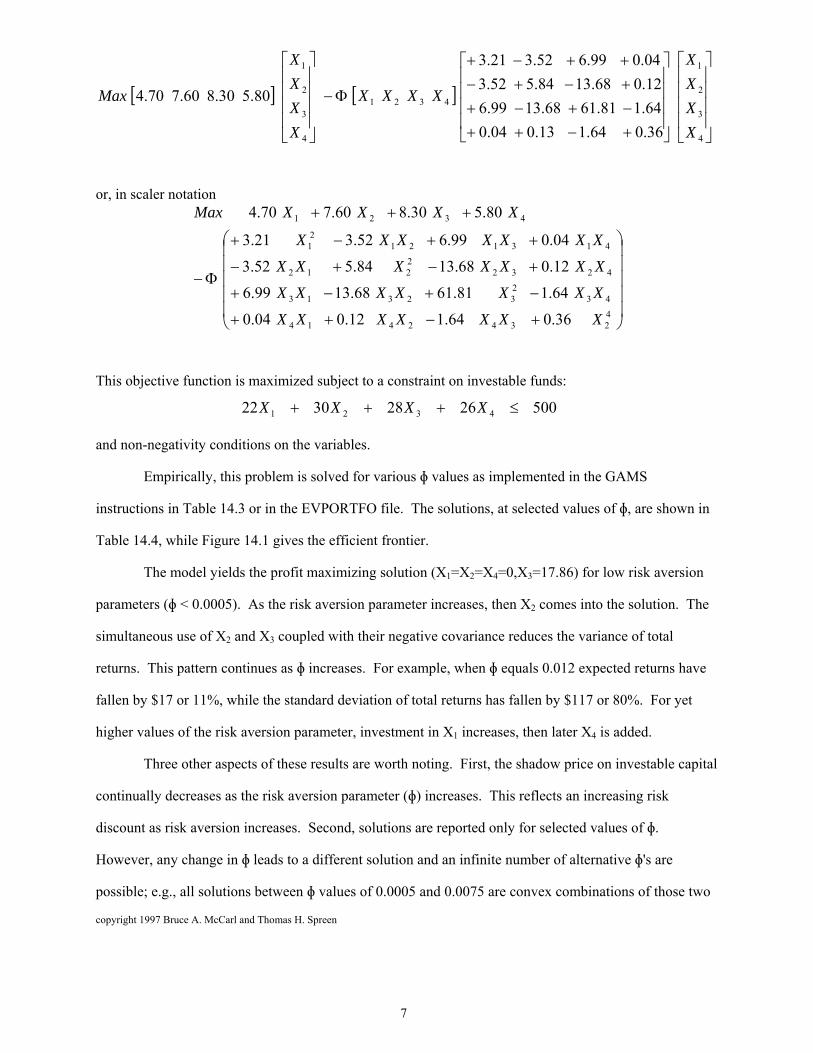
14.3.1.1.1 Example
Assume an investor wishes to develop a stock portfolio given the stock annual returns
information shown in Table 14.1, 500 dollars to invest and prices of stock one $22.00, stock two $30.00,
stock three $28.00 and stock four $26.00.
The first stage in model application is to compute average returns and the variance-covariance
matrix of total net returns. The mean returns and variance - covariance matrix are shown in Table 14.2.
In turn the objective function is
jallfor0X
1Xs.t.
XXsXcMax
j
jj
j kkjjk
jjj
X)c(
)
0X
bAXs.t.
SXXXCMax
C
copyright 1997 Bruce A. McCarl and Thomas H. Spreen
7
4
3
2
1
4321
4
3
2
1
36.064.113.004.0
64.181.6168.1399.6
12.068.1384.552.3
04.099.652.321.3
80.530.860.770.4
X
X
X
X
XXXX
X
X
X
X
Max
or, in scaler notation
42342414
43232313
42322212
4131212
1
4321
36.064.112.004.0
64.181.6168.1399.6
12.068.1384.552.3
04.099.652.321.3
80.530.860.770.4
XXXXXXX
XXXXXXX
XXXXXXX
XXXXXXX
XXXXMax
This objective function is maximized subject to a constraint on investable funds:
50026283022 4321 XXXX
and non-negativity conditions on the variables.
Empirically, this problem is solved for various ɸ values as implemented in the GAMS
instructions in Table 14.3 or in the EVPORTFO file. The solutions, at selected values of ɸ, are shown in
Table 14.4, while Figure 14.1 gives the efficient frontier.
The model yields the profit maximizing solution (X1=X2=X4=0,X3=17.86) for low risk aversion
parameters (ɸ < 0.0005). As the risk aversion parameter increases, then X2 comes into the solution. The
simultaneous use of X2 and X3 coupled with their negative covariance reduces the variance of total
returns. This pattern continues as ɸ increases. For example, when ɸ equals 0.012 expected returns have
fallen by $17 or 11%, while the standard deviation of total returns has fallen by $117 or 80%. For yet
higher values of the risk aversion parameter, investment in X1 increases, then later X4 is added.
Three other aspects of these results are worth noting. First, the shadow price on investable capital
continually decreases as the risk aversion parameter (ɸ) increases. This reflects an increasing risk
discount as risk aversion increases. Second, solutions are reported only for selected values of ɸ.
However, any change in ɸ leads to a different solution and an infinite number of alternative ɸ's are
possible; e.g., all solutions between ɸ values of 0.0005 and 0.0075 are convex combinations of those two
copyright 1997 Bruce A. McCarl and Thomas H. Spreen
8
solutions. Third, when ɸ becomes sufficiently large, the model does not use all its resources. In this
particular case, when ɸ exceeds 2.5, not all funds are invested.
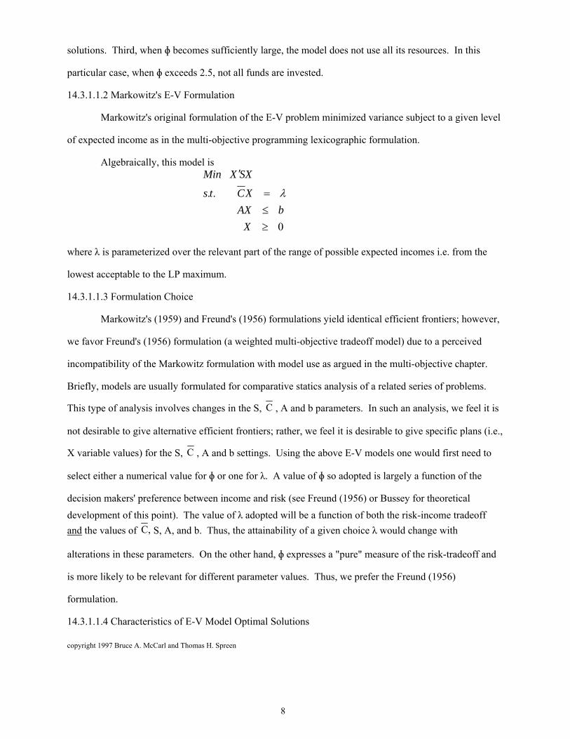
14.3.1.1.2 Markowitz's E-V Formulation
Markowitz's original formulation of the E-V problem minimized variance subject to a given level
of expected income as in the multi-objective programming lexicographic formulation.
Algebraically, this model is
0
..
X
bAX
XCts
SXXMin
where λ is parameterized over the relevant part of the range of possible expected incomes i.e. from the
lowest acceptable to the LP maximum.
14.3.1.1.3 Formulation Choice
Markowitz's (1959) and Freund's (1956) formulations yield identical efficient frontiers; however,
we favor Freund's (1956) formulation (a weighted multi-objective tradeoff model) due to a perceived
incompatibility of the Markowitz formulation with model use as argued in the multi-objective chapter.
Briefly, models are usually formulated for comparative statics analysis of a related series of problems.
This type of analysis involves changes in the S, , A and b parameters. In such an analysis, we feel it is
not desirable to give alternative efficient frontiers; rather, we feel it is desirable to give specific plans (i.e.,
X variable values) for the S, , A and b settings. Using the above E-V models one would first need to
select either a numerical value for ɸ or one for λ. A value of ɸ so adopted is largely a function of the
decision makers' preference between income and risk (see Freund (1956) or Bussey for theoretical
development of this point). The value of λ adopted will be a function of both the risk-income tradeoff
and the values of S, A, and b. Thus, the attainability of a given choice λ would change with
alterations in these parameters. On the other hand, ɸ expresses a "pure" measure of the risk-tradeoff and
is more likely to be relevant for different parameter values. Thus, we prefer the Freund (1956)
formulation.
14.3.1.1.4 Characteristics of E-V Model Optimal Solutions
C
C
,C
copyright 1997 Bruce A. McCarl and Thomas H. Spreen
9
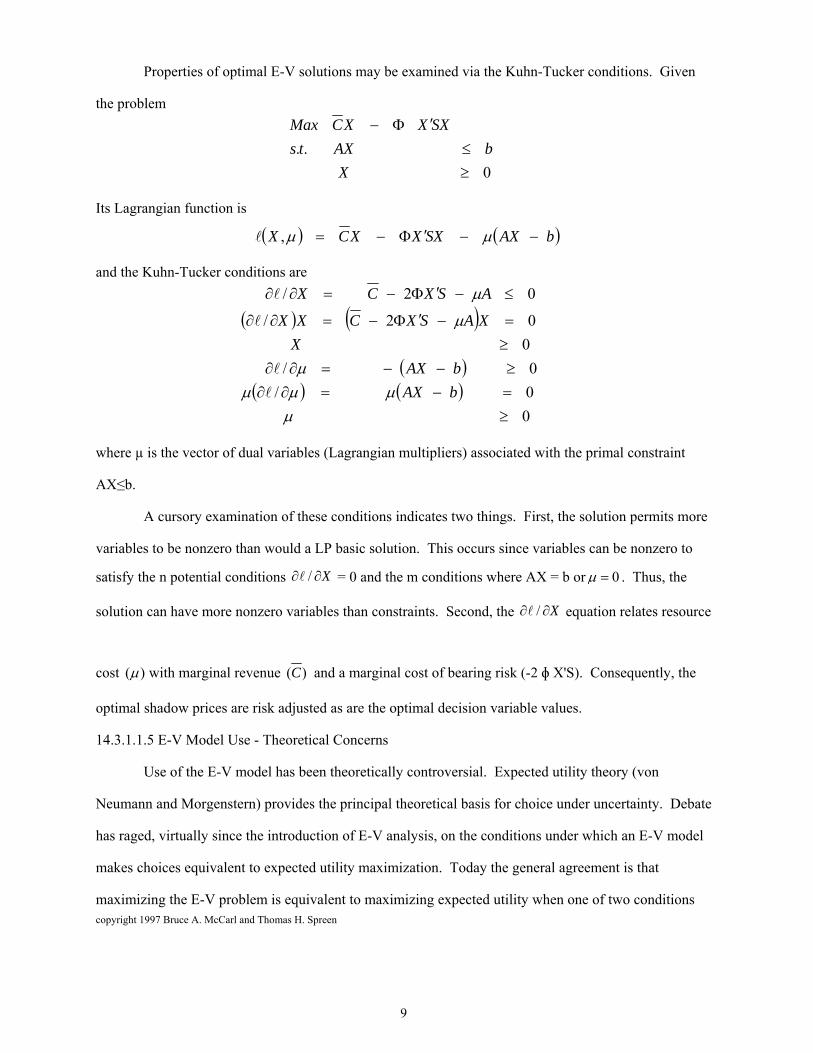
Properties of optimal E-V solutions may be examined via the Kuhn-Tucker conditions. Given
the problem
0
..
X
bAXts
SXXXCMax
Its Lagrangian function is
bAXSXXXCX ,
and the Kuhn-Tucker conditions are
0
0/
0/
0
02/
02/
bAX
bAX
X
XASXCXX
ASXCX
where µ is the vector of dual variables (Lagrangian multipliers) associated with the primal constraint
AX≤b.
A cursory examination of these conditions indicates two things. First, the solution permits more
variables to be nonzero than would a LP basic solution. This occurs since variables can be nonzero to
satisfy the n potential conditions = 0 and the m conditions where AX = b or . Thus, the
solution can have more nonzero variables than constraints. Second, the equation relates resource
cost with marginal revenue and a marginal cost of bearing risk (-2 ɸ X'S). Consequently, the
optimal shadow prices are risk adjusted as are the optimal decision variable values.
14.3.1.1.5 E-V Model Use - Theoretical Concerns
Use of the E-V model has been theoretically controversial. Expected utility theory (von
Neumann and Morgenstern) provides the principal theoretical basis for choice under uncertainty. Debate
has raged, virtually since the introduction of E-V analysis, on the conditions under which an E-V model
makes choices equivalent to expected utility maximization. Today the general agreement is that
maximizing the E-V problem is equivalent to maximizing expected utility when one of two conditions
X / 0
X /
)( )(C
copyright 1997 Bruce A. McCarl and Thomas H. Spreen
10
hold: 1) the underlying income distribution is normal - which requires a normal distribution of the cj and
the utility function is exponential (Freund, 1956; Bussey)4, and 2) the underlying distributions satisfy
Meyer's location and scale restrictions. In addition, Tsiang (1972, 1974) has shown that E-V analysis
provides an acceptable approximation of the expected utility choices when the risk taken is small relative
to total initial wealth. The E-V frontier has also been argued to be appropriate under quadratic utility
(Tobin). There have also been empirical studies (Levy and Markowitz; Kroll, et al.; and Reid and Tew)
wherein the closeness of E-V to expected utility maximizing choices has been shown.
14.3.1.1.6 Specification of the Risk Aversion Parameter
E-V models need numerical risk aversion parameters (ɸ). A number of approaches have been
used for parameter specification. First, one may avoid specifying a value and derive the efficient frontier.
This involves solving for many possible risk aversion parameters. Second, one may derive the efficient
frontier and present it to a decision maker who picks an acceptable point (ideally, where his utility
function and the E-V frontier are tangent) which in turn identifies a specific risk aversion parameter
(Candler and Boeljhe). Third, one may assume that the E-V rule was used by decision makers in
generating historical choices, and can fit the risk aversion parameter as equal to the difference between
marginal revenue and marginal cost of resources, divided by the appropriate marginal variance (Weins).
Fourth, one may estimate a risk aversion parameter such that the difference between observed behavior
and the model solution is minimized (as in Brink and McCarl (1979) or Hazell et al. (1983)). Fifth, one
may subjectively elicit a risk aversion parameter (see Anderson, et al. for details) and in turn fit it into the
objective function (i.e., given a Pratt risk aversion coefficient and assuming exponential utility implies the
E-V ɸ equals 1/2 the Pratt risk aversion coefficient [Freund, 1956 or Bussey]). Sixth, one may transform
a risk aversion coefficient from another study or develop one based on probabilistic assumptions (McCarl
and Bessler).
The E-V model has a long history. The earliest application appears to be Freund's (1956). Later,
Heady and Candler; McFarquhar; and Stovall all discussed possible uses of this methodology. A sample 4 Normality probably validates a larger class of utility functions but only the exponential case has
been worked out.

copyright 1997 Bruce A. McCarl and Thomas H. Spreen
11
of applications includes those of Brainard and Cooper; Lin, et al.; and Wiens. In addition, numerous
references can be found in Boisvert and McCarl; Robinson and Brake; and Barry.
14.3.1.2 A Linear Approximation - MOTAD
The E-V model yields a quadratic programming problem. Such problems traditionally have been
harder to solve than linear programs (although McCarl and Onal argue this is no longer true). Several LP
approximations have evolved (Hazell, 1971; Thomas et al; Chen and Baker; and others as reviewed in
McCarl and Tice). Only Hazell's MOTAD is discussed here due to its extensive use.
The acronym MOTAD refers to Minimization of Total Absolute Deviations. In the MOTAD
model, absolute deviation is the risk measure. Thus, the MOTAD model depicts tradeoffs between
expected income and the absolute deviation of income. Minimization of absolute values is discussed in
the nonlinear approximations chapter. Briefly reviewing, absolute value may be minimized by
constraining the terms whose absolute value is to be minimized (Dk) equal to the difference of two
non-negative variables ( Dk = dk+ - dk
- ) and in turn minimizing the sum of the new variables ∑ ( dk+ + dk
-).
Hazell(1971) used this formulation in developing the MOTAD model.5
Formally, the total absolute deviation of income from mean income under the kth state of nature
(Dk) is
jj
jjkj
jk XcXcD
where ckj is the per unit net return to Xj under the kth state of nature and is the mean.
Since both terms involve Xj and sum over the same index, this can be rewritten as
jjkjj
k XccD
Total absolute deviation (TAD) is the sum of Dk across the states of nature. Now introducing
deviation variables to depict positive and negative deviations we get
5 The approach was suggested in Markowitz (1959, p. 187).
jc
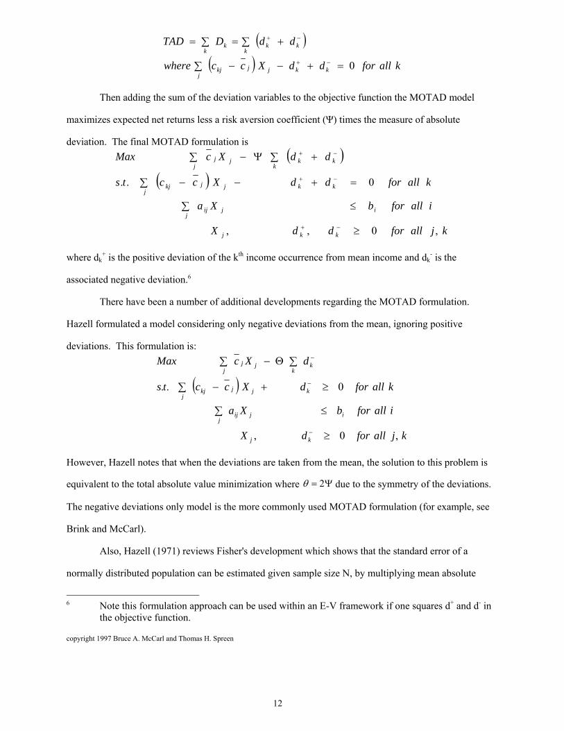
copyright 1997 Bruce A. McCarl and Thomas H. Spreen
12
kallforddXccwhere
ddDTAD
kkjjkjj
kkk
kk
0
Then adding the sum of the deviation variables to the objective function the MOTAD model
maximizes expected net returns less a risk aversion coefficient (Ψ) times the measure of absolute
deviation. The final MOTAD formulation is
kjallforddX
iallforbXa
kallforddXccts
ddXcMax
kkj
ijijj
kkjjkjj
kkk
jjj
,0,,
0..
where dk+ is the positive deviation of the kth income occurrence from mean income and dk
- is the
associated negative deviation.6
There have been a number of additional developments regarding the MOTAD formulation.
Hazell formulated a model considering only negative deviations from the mean, ignoring positive
deviations. This formulation is:
kjallfordX
iallforbXa
kallfordXccts
dXcMax
kj
ijijj
kjjkjj
kk
jjj
,0,
0..
However, Hazell notes that when the deviations are taken from the mean, the solution to this problem is
equivalent to the total absolute value minimization where due to the symmetry of the deviations.
The negative deviations only model is the more commonly used MOTAD formulation (for example, see
Brink and McCarl).
Also, Hazell (1971) reviews Fisher's development which shows that the standard error of a
normally distributed population can be estimated given sample size N, by multiplying mean absolute
6 Note this formulation approach can be used within an E-V framework if one squares d+ and d- in
the objective function.
2
copyright 1997 Bruce A. McCarl and Thomas H. Spreen
13
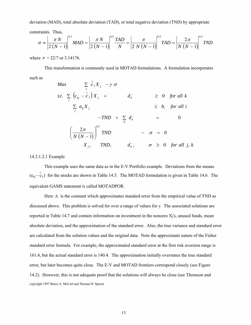
deviation (MAD), total absolute deviation (TAD), or total negative deviation (TND) by appropriate
constraints. Thus,
TNDNN
TADNNN
TAD
N
NMAD
N
N5.05.05.05.0
1
2
121212
where = 22/7 or 3.14176.
This transformation is commonly used in MOTAD formulations. A formulation incorporates
such as
kjallfordTNDX
TNDNN
dTND
iallforbXa
kallfordXccts
XcMax
kj
kk
ijijj
kjjkjj
jjj
,0,,,
01
2
0
0..
5.0
14.3.1.2.1 Example
This example uses the same data as in the E-V Portfolio example. Deviations from the means
(ckj for the stocks are shown in Table 14.5. The MOTAD formulation is given in Table 14.6. The
equivalent GAMS statement is called MOTADPOR.
Here is the constant which approximates standard error from the empirical value of TND as
discussed above. This problem is solved for over a range of values for γ. The associated solutions are
reported in Table 14.7 and contain information on investment in the nonzero Xj's, unused funds, mean
absolute deviation, and the approximation of the standard error. Also, the true variance and standard error
are calculated from the solution values and the original data. Note the approximate nature of the Fisher
standard error formula. For example, the approximated standard error at the first risk aversion range is
161.4, but the actual standard error is 140.4. The approximation initially overstates the true standard
error, but later becomes quite close. The E-V and MOTAD frontiers correspond closely (see Figure
14.2). However, this is not adequate proof that the solutions will always be close (see Thomson and
)c j

copyright 1997 Bruce A. McCarl and Thomas H. Spreen
14
Hazell for a comparison between the methods).
14.3.1.2.2 Comments on MOTAD
Many of the E-V model comments are appropriate here and will not be repeated. However, a
number of other comments are in order. First, a cursory examination of the MOTAD model might lead
one to conclude covariance is ignored. This is not so. The deviation equations add across all the
variables, allowing negative deviation in one variable to cancel positive deviation in another. Thus, in
minimizing total absolute deviation the model has an incentive to "diversify", taking into account
covariance.
Second, the equivalence of the total negative and total absolute deviation formulations depends
critically upon deviation symmetry. Symmetry will occur whenever the deviations are taken from the
mean. This, however, implies that the mean is the value expected for each observation. This may not
always be the case. When the value expected is not the mean, then moving averages or other expectation
models should be used instead of the mean (see Brink and McCarl, or Young). In such cases, the
deviations are generally non-symmetric and consideration must be given to an appropriate measure of
risk. For example, Brink and McCarl use a mean negative deviation formulation with a moving average
expectation.
Third, most MOTAD applications use approximated standard errors as a measure of risk. When
using such a measure, the risk aversion parameters can be interpreted as the number of standard errors one
wishes to discount income. Coupling this with a normality assumption permits one to associate a
confidence limit with the risk aversion parameter. For example, a risk aversion parameter equal to one
means that level of income which occurs at one standard error below the mean is maximized. Assuming
normality, this level of income is 84% sure to occur.
Fourth, one must have empirical values for the risk aversion parameter. All the E-V approaches
are applicable to its discovery. The most common approach with MOTAD models has been based on
observed behavior. The procedure has been to: a) take a vector of observed solution variables, (i.e.
acreages); b) parameterize the risk aversion coefficient in small steps (e.g., 0.25) from 0 to 2.5, at each
point computing a measure of the difference between the model solution and observed behavior; and c)

copyright 1997 Bruce A. McCarl and Thomas H. Spreen
15
select the risk aversion parameter value for which the smallest dispersion is found between the model
solution values and the observed values (for examples see Hazell et al.; Brink and McCarl; Simmons and
Pomareda; or Nieuwoudt, et al.).
Fifth, the MOTAD model does not have a general direct relationship to a theoretical utility
function. Some authors have discovered special cases under which there is a link (see Johnson and
Boeljhe(1981,1983) and their subsequent exchange with Buccola). Largely, the MOTAD model has been
presented as an approximation to the E-V model. However, with the advances in nonlinear programming
algorithms the approximation motivation is largely gone (McCarl and Onal), but MOTAD may have
application to non-normal cases (Thomson and Hazell).
Sixth, McCarl and Bessler derive a link between the E-standard error and E-V risk aversion
parameters as follows:
Consider the models
00
....
2
XX
bAXtsversusbAXts
XcXMaxXcXMax
The first order conditions assuming X is nonzero are
002
A
X
XcA
X
XXc
For these two solutions to be identical in terms of X and �, then
X
2
Thus, the E-V risk aversion coefficient will equal the E-standard error model risk aversion coefficient
divided by twice the standard error. This explains why E-V risk aversion coefficients are usually very
small (i.e., an E-standard error risk aversion coefficient usually ranges from 0 - 3 which implies when the
standard error of income is $10,000 the E-V risk aversion coefficient range of 0 - .000015).
Unfortunately, since is a function of which depends on X, this condition must hold ex post and
cannot be imposed a priori. However, one can develop an approximate a priori relationship between the
risk aversion parameters given an estimate of the standard error.
The seventh and final comment regards model sensitivity. Schurle and Erven show that several
copyright 1997 Bruce A. McCarl and Thomas H. Spreen
16
plans with very different solutions can be feasible and close to the plans on the efficient frontier. Both
results place doubt on strict adherence to the efficient frontier as a norm for decision making. (Actually
the issue of near optimal solutions is much broader than just its role in risk models.) The MOTAD model
has been rather widely used. Early uses were by Hazell (1971); Hazell and Scandizzo; Hazell et al.
(1983); Simmons and Pomareda; and Nieuwoudt, et al. In the late 1970's the model saw much use.
Articles from 1979 through the mid 1980s in just the American Journal of Agricultural Economics
include Gebremeskel and Shumway; Schurle and Erven; Pomareda and Samayoa; Mapp, et al.; Apland, et
al. (1980); and Jabara and Thompson. Boisvert and McCarl provide a recent review.
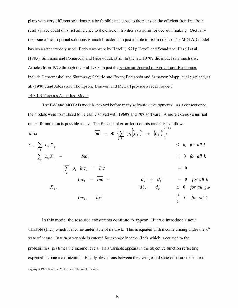
14.3.1.3 Towards A Unified Model
The E-V and MOTAD models evolved before many software developments. As a consequence,
the models were formulated to be easily solved with 1960's and 70's software. A more extensive unified
model formulation is possible today. The E-standard error form of this model is as follows
kallforIncInc
kjallforddX
kallforddIncInc
IncIncp
kallforIncXc
iallforbXcts
ddpincMax
k
kkj
kkk
kkk
kjkjj
ijkjj
kkkk
0,
,0,,
0
0
0
..
5.022
In this model the resource constraints continue to appear. But we introduce a new
variable (Inck) which is income under state of nature k. This is equated with income arising under the kth
state of nature. In turn, a variable is entered for average income which is equated to the
probabilities (pk) times the income levels. This variable appears in the objective function reflecting
expected income maximization. Finally, deviations between the average and state of nature dependent
)Inc(
copyright 1997 Bruce A. McCarl and Thomas H. Spreen
17
income levels are treated in deviation constraints where dk+ indicates income above the average level
whereas dk- indicates shortfalls. The objective function is then modified to include the probabilities and
deviation variables. Several possible objective function formulations are possible. The objective function
formulation above is E-standard error without approximation. Note that the term in parentheses contains
the summed, probabilistically weighted, squared deviations from the mean and is by definition equal to
the variance. In turn, the square root of this term is the standard deviation and � would be a risk aversion
parameter which would range between zero and 2.5 in most circumstances (as explained in the MOTAD
section).
This objective function can also be reformulated to be equivalent to either the MOTAD or E-V
cases. Namely, in the E-V case if we drop the 0.5 exponent then the bracketed term is variance and the
model would be E-V. Similarly, if we drop the 0.5 exponent and do not square the deviation variables
then a MOTAD model arises.
This unifying framework shows how the various models are related and indicates that covariance
is considered in any of the models. An example is not presented here although the files UNIFY, EV2 and
MOTAD2 give GAMS implementations of the unified E-standard error, E-V and MOTAD versions. The
resultant solutions are identical to the solution for E-V and MOTAD examples and are thus not discussed
further.
14.3.1.4 Safety First
Roy posed a different approach to handling objective function uncertainty. This approach, the
Safety First model, assumes that decision makers will choose plans to first assure a given safety level for
income. The formulation arises as follows: assume the model income level under all k states of nature
(∑ckj Xj ) must exceed the safety level (S). This can be assured by entering the constraints kallforSXc jkj
j
The overall problem then becomes
copyright 1997 Bruce A. McCarl and Thomas H. Spreen
18
jallforX
kallforSXc
iallforbXats
XcMax
j
jkjj
ijijj
jjj
0
..
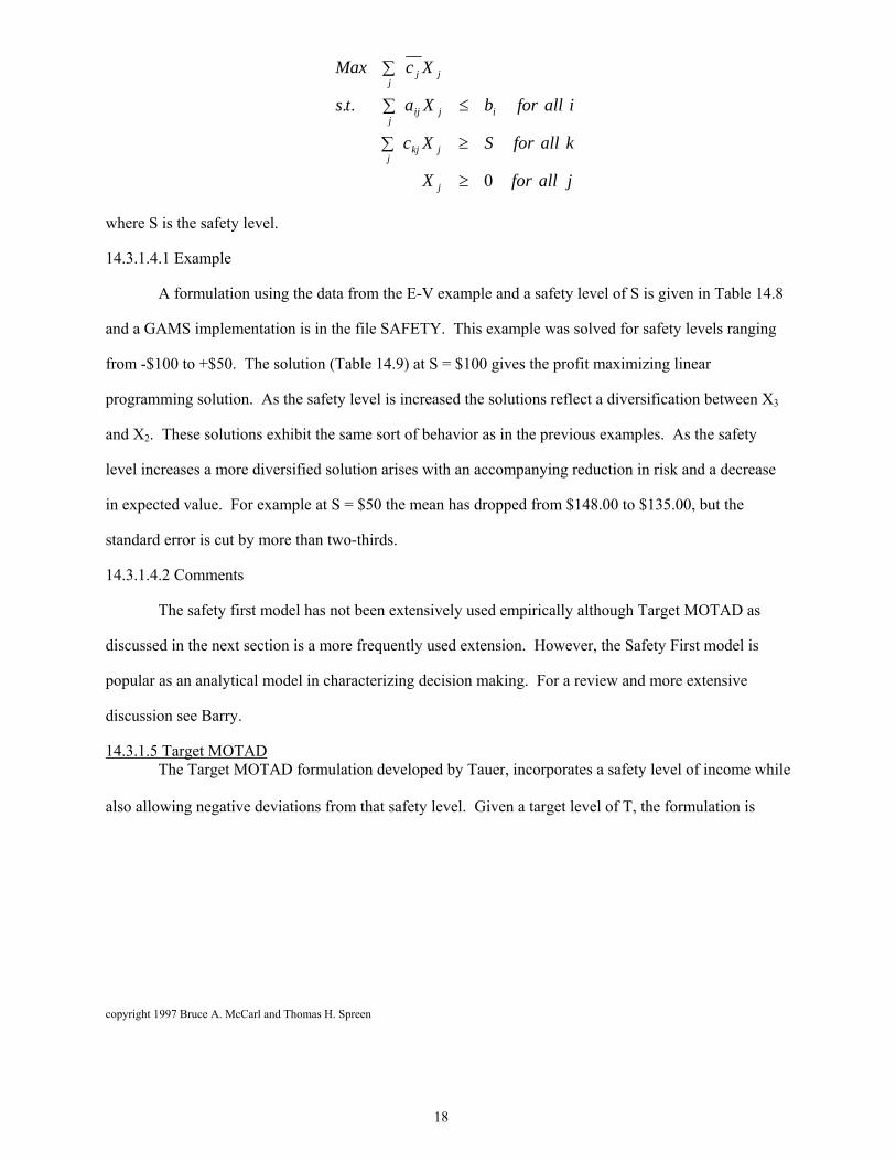
where S is the safety level.
14.3.1.4.1 Example
A formulation using the data from the E-V example and a safety level of S is given in Table 14.8
and a GAMS implementation is in the file SAFETY. This example was solved for safety levels ranging
from -$100 to +$50. The solution (Table 14.9) at S = $100 gives the profit maximizing linear
programming solution. As the safety level is increased the solutions reflect a diversification between X3
and X2. These solutions exhibit the same sort of behavior as in the previous examples. As the safety
level increases a more diversified solution arises with an accompanying reduction in risk and a decrease
in expected value. For example at S = $50 the mean has dropped from $148.00 to $135.00, but the
standard error is cut by more than two-thirds.
14.3.1.4.2 Comments
The safety first model has not been extensively used empirically although Target MOTAD as
discussed in the next section is a more frequently used extension. However, the Safety First model is
popular as an analytical model in characterizing decision making. For a review and more extensive
discussion see Barry.
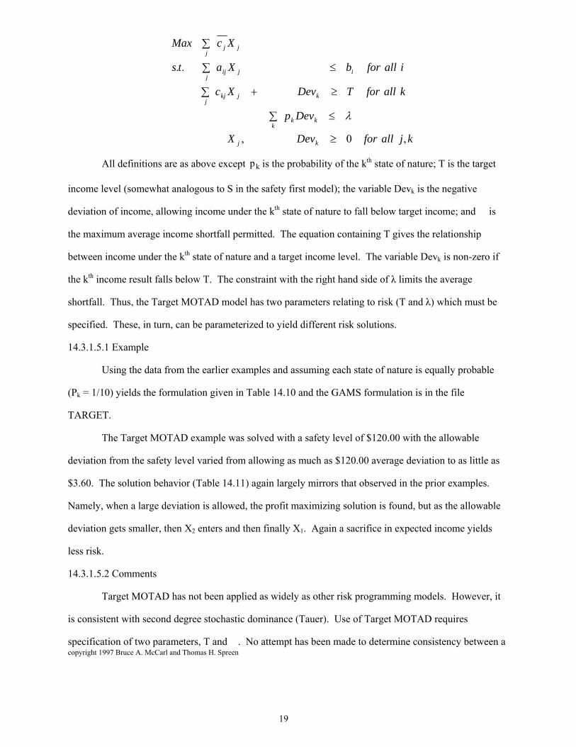
14.3.1.5 Target MOTAD The Target MOTAD formulation developed by Tauer, incorporates a safety level of income while also allowing negative deviations from that safety level. Given a target level of T, the formulation is
copyright 1997 Bruce A. McCarl and Thomas H. Spreen
19
kjallforDevX
Devp
kallforTDevXc
iallforbXats
XcMax
kj
kkk
kjkjj
ijijj
jjj
,0,
..
All definitions are as above except is the probability of the kth state of nature; T is the target
income level (somewhat analogous to S in the safety first model); the variable Devk is the negative
deviation of income, allowing income under the kth state of nature to fall below target income; and � is
the maximum average income shortfall permitted. The equation containing T gives the relationship
between income under the kth state of nature and a target income level. The variable Devk is non-zero if
the kth income result falls below T. The constraint with the right hand side of λ limits the average
shortfall. Thus, the Target MOTAD model has two parameters relating to risk (T and λ) which must be
specified. These, in turn, can be parameterized to yield different risk solutions.
14.3.1.5.1 Example
Using the data from the earlier examples and assuming each state of nature is equally probable
(Pk = 1/10) yields the formulation given in Table 14.10 and the GAMS formulation is in the file
TARGET.
The Target MOTAD example was solved with a safety level of $120.00 with the allowable
deviation from the safety level varied from allowing as much as $120.00 average deviation to as little as
$3.60. The solution behavior (Table 14.11) again largely mirrors that observed in the prior examples.
Namely, when a large deviation is allowed, the profit maximizing solution is found, but as the allowable
deviation gets smaller, then X2 enters and then finally X1. Again a sacrifice in expected income yields
less risk.
14.3.1.5.2 Comments
Target MOTAD has not been applied as widely as other risk programming models. However, it
is consistent with second degree stochastic dominance (Tauer). Use of Target MOTAD requires
specification of two parameters, T and �. No attempt has been made to determine consistency between a
kp
copyright 1997 Bruce A. McCarl and Thomas H. Spreen
20
T, λ choice and the Arrow-Pratt measure of risk aversion. Nor is there theory on how to specify T and λ.
The target MOTAD and original MOTAD models can be related. If one makes λ a variable with a cost in
the objective function and makes the target level a variable equal to expected income, this becomes the
MOTAD model.
Another thing worth noting is that the set of Target MOTAD solutions are continuous so that
there is an infinite number of solutions. In the example, any target deviation between $24.00 and $12.00
would be a unique solution and would be a convex combination of the two tabled solutions.
McCamley and Kliebenstein outline a strategy for generating all target MOTAD solutions, but it
is still impossible to relate these solutions to more conventional measures of risk preferences.
Target MOTAD has been used in a number of contexts. Zimet and Spreen formulate a farm
production implementation while Curtis et al., and Frank et al., studied crop marketing problems.
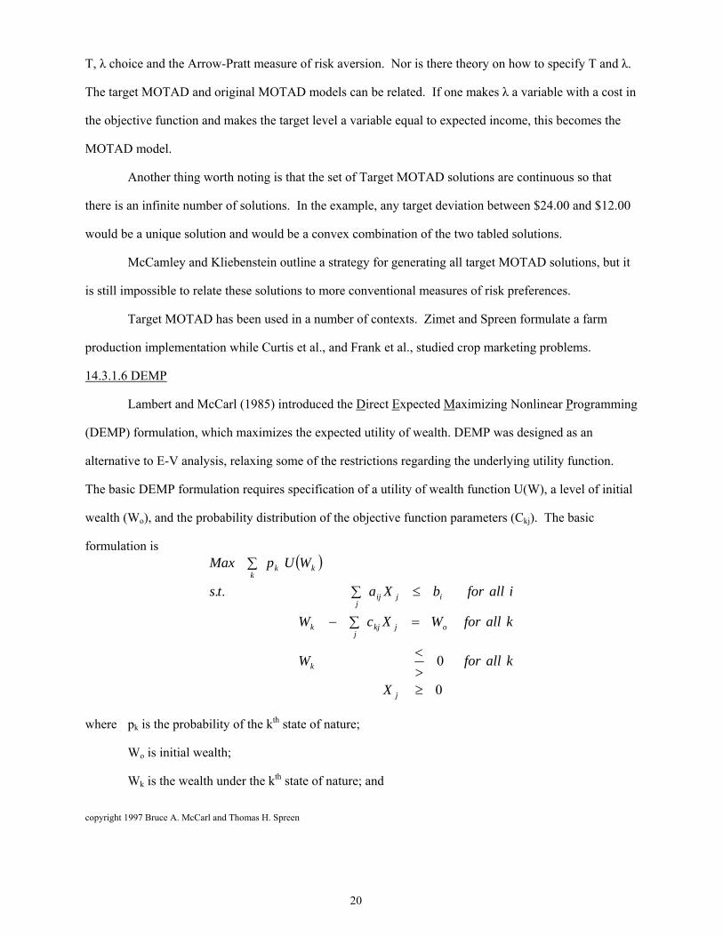
14.3.1.6 DEMP
Lambert and McCarl (1985) introduced the Direct Expected Maximizing Nonlinear Programming
(DEMP) formulation, which maximizes the expected utility of wealth. DEMP was designed as an
alternative to E-V analysis, relaxing some of the restrictions regarding the underlying utility function.
The basic DEMP formulation requires specification of a utility of wealth function U(W), a level of initial
wealth (Wo), and the probability distribution of the objective function parameters (Ckj). The basic
formulation is
0
0
..
j
k
ojkjj
k
ijijj
kkk
X
kallforW
kallforWXcW
iallforbXats
WUpMax
where pk is the probability of the kth state of nature;
Wo is initial wealth;
Wk is the wealth under the kth state of nature; and

copyright 1997 Bruce A. McCarl and Thomas H. Spreen
21
ckj is the return to one unit of the jth activity under the kth state of nature.
14.3.1.6.1 Example
Suppose an individual has the utility function for wealth of the form U = ( W) power with an initial
wealth (W0) of 100, and is confronted with the decision problem data as used in the E-V example. The
relevant DEMP formulation appears in Table 14.12 with the solution for varying values of the exponent
appearing in Table 14.13. The GAMS formulation is called DEMP.
The example model was solved for different values of the exponent (power). The exponent was
varied from 0.3 to 0.0001. As this was varied, the solution again transitioned out of sole reliance on stock
three into reliance on stocks two and three. During the model calculations, transformations were done on
the shadow price to convert it into dollars. Following Lambert and McCarl, this may be converted into an
approximate value in dollar space by dividing by the marginal utility of average income i.e., dividing the
shadow prices by the factor.
W
WU
/*
Preckel, Featherstone, and Baker discuss a variant of this procedure.
14.3.1.6.2 Comments
The DEMP model has two important parts. First, note that the constraints involving wealth can
be rearranged to yield
jkjj
ok XcWW
This sets wealth under the kth state of nature equal to initial wealth plus the increment to wealth due to the
choice of the decision variables.
Second, note that the objective function equals expected utility. Thus the formulation maximizes
expected utility using the empirical distribution of risk without any distributional form assumptions and
an explicit, exact specification of the utility function.
Kaylen, et al., employ a variation of DEMP where the probability distributions are of a known
continuous form and numerical integration is used in the solution. The DEMP model has been used by
Lambert and McCarl(1989); Lambert; and Featherstone et al.

copyright 1997 Bruce A. McCarl and Thomas H. Spreen
22
Yassour, et al., present a related expected utility maximizing model called EUMGF, which
embodies both an exponential utility function and distributional assumptions. They recognize that the
maximization of expected utility under an exponential utility function is equivalent to maximization of the
moment generating function (Hogg and Craig) for a particular probability distribution assumption.
Moment generating functions have been developed analytically for a number of distributions, including
the Binomial, Chi Square, Gamma, Normal and Poisson distributions. Collender and Zilberman and
Moffit et al. have applied the EUMGF model. Collender and Chalfant have proposed a version of the
model no longer requiring that the form of the probability distribution be known.
14.3.1.7 Other Formulations
The formulations mentioned above are the principal objective function risk formulations which
have been used in applied mathematical programming risk research. However, a number of other
formulations have been proposed. Alternative portfolio models such as those by Sharpe; Chen and Baker;
Thomas et al.(1972) exist. Other concepts of target income have also been pursued (Boussard and Petit)
as have models based upon game theory concepts (McInerney [1967, 1969]; Hazell and How; Kawaguchi
and Maruyama; Hazell(1970); Agrawal and Heady; Maruyama; and Low) and Gini coefficients
(Yitzhaki). These have all experienced very limited use and are therefore not covered herein.
14.3.2 Right Hand Side Risk
Risk may also occur within the right hand side (RHS) parameters. The most often used approach
to RHS risk in a nonrecourse setting is chance-constrained programming. However, Paris(1979) has tried
to introduce an alternative.
14.3.2.1 Chance Constrained Programming
The chance-constrained formulation was introduced by Charnes and Cooper and deals with
uncertain RHS's assuming the decision maker is willing to make a probabilistic statement about the
frequency with which constraints need to be satisfied. Namely, the probability of a constraint being
satisfied is greater than or equal to a prespecified value
ijij
jbXaP
.

copyright 1997 Bruce A. McCarl and Thomas H. Spreen
23
If the average value of the RHS is subtracted from both sides of the inequality and in turn both
sides are divided by the standard deviation of the RHS then the constraint becomes
ib
ii
ib
ijijj bb
bXaP
Those familiar with probability theory will note that the term
ib
ii bb
gives the number of standard errors that bi is away from the mean. Let Z denote this term.
When a particular probability limit α is used, then the appropriate value of Z is Z� and the
constraint becomes
Z
bXaP
ib
ijijj
Assuming we discount for risk, then the constraint can be restated as
ibijijj
ZbXa
which states that resource use (∑aijXj) must be less than or equal to average resource availability less the
standard deviation times a critical value which arises from the probability level.
Values of Zα may be determined in two ways: a) by making assumptions about the form of the
probability distribution of bi (for example, assuming normality and using values for the lower tail from a
standard normal probability table); or b) by relying on the conservative estimates generated by using
Chebyshev's inequality, which states the probability of an estimate falling greater than M standard
deviations away from the mean is less than or equal to one divided by M2. Using the Chebyshev
inequality one needs to solve for that value of M such that (1-α) equals 1/M2. Thus, given a probability α,
)b( i
ib

copyright 1997 Bruce A. McCarl and Thomas H. Spreen
24
the Chebyshev value of Zα is given by the equation Zα=(1-α)-0.5. Following these approaches, if one
wished an 87.5 percent probability, a normality assumption would discount 1.14 standard deviations and
an application of the Chebyshev inequality would lead to a discount of 2.83 standard deviations.
However, one should note that the Chebyshev bound is often too large.
14.3.2.1.1 Example
The example problem adopted for this analysis is in the context of the resource allocation
problem from Chapter V. Here three of the four right hand sides in that problem are presumed to be
stochastic with the distribution as given in Table 14.14. Treating each of these right hand side
observations as equally likely, the mean value equals those numbers that were used in the resource
allocation problem and their standard errors respectively are as given in Table 14.14. Then the resultant
chance constrained formulation is Max 67X1 + 66X2 + 66.3X3 + 80X4 + 78.5X5 + 78.4X6
s.t 0.8X1 + 1.3X2 + 0.2X3 + 1.2X4 + 1.7X5 + 0.5X6 ≤ 140 - 9.63 Zα
0.5X1 + 0.2X2 + 1.3X3 + 0.7X4 + 0.3X5 + 1.5X6 ≤ 90 - 3.69 Zα
0.4X1 + 0.4X2 + 0.4X3 + X4 + X5 + X6 ≤ 120 - 8.00 Zα
X1 + 1.05X2 + 1.1X3 + 0.8X4 + 0.82X5 + 0.84X6 ≤ 125
The GAMS implementation is the file CHANCE. The solutions to this model were run for Z
values corresponding to 0, 90 ,95, and 99 percent confidence intervals under a normality assumption. The
right hand sides and resultant solutions are tabled in Table 14.15. Notice as the Zα value is increased, then
the value of the uncertain right hand side decreases. In turn, production decreases as does profit. The
chance constrained model discounts the resources available, so one is more certain that the constraint will
be met. The formulation also shows how to handle simultaneous constraints. Namely the constraints
may be treated individually. Note however this requires an assumption that the right hand sides are
completely independent. The results also show that there is a chance of the constraints being exceeded
but no adjustment is made for what happens under that circumstance.
14.3.2.1.2 Comments
copyright 1997 Bruce A. McCarl and Thomas H. Spreen
25
Despite the fact that chance constrained programming (CCP) is a well known technique and has
been applied to agriculture (e.g., Boisvert, 1976; Boisvert and Jensen, 1973; and Danok et al., 1980) and
water management (e.g., Eisel; Loucks; and Maji and Heady) its use has been limited and controversial.
See the dialogue in Blau; Hogan, et al.; and Charnes and Cooper (1959).
The major advantage of CCP is its simplicity; it leads to an equivalent programming problem of
about the same size and the only additional data requirements are the standard errors of the right hand
side. However, its only decision theoretic underpinning is Simon's principle of satisficing (Pfaffenberger
and Walker).
This CCP formulation applies when either one element of the right hand side vector is random or
when the distribution of multiple elements is assumed to be perfectly correlated. The procedure has been
generalized to other forms of jointly distributed RHS's by Wagner (1975). A fundamental problem with
chance constrained programming (CCP) is that it does not indicate what to do if the recommended
solution is not feasible. From this perspective, Hogan et al., (1981), conclude that "... there is little
evidence that CCP is used with the care that is necessary" (p. 698) and assert that recourse formulations
should be used.
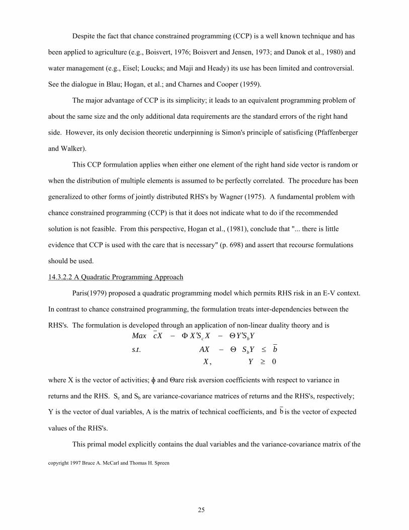
14.3.2.2 A Quadratic Programming Approach
Paris(1979) proposed a quadratic programming model which permits RHS risk in an E-V context.
In contrast to chance constrained programming, the formulation treats inter-dependencies between the
RHS's. The formulation is developed through an application of non-linear duality theory and is
0,
..
YX
bYSAXts
YSYXSXXcMax
b
bc
where X is the vector of activities; ɸ and Θare risk aversion coefficients with respect to variance in
returns and the RHS. Sc and Sb are variance-covariance matrices of returns and the RHS's, respectively;
Y is the vector of dual variables, A is the matrix of technical coefficients, and is the vector of expected
values of the RHS's.
This primal model explicitly contains the dual variables and the variance-covariance matrix of the
b

copyright 1997 Bruce A. McCarl and Thomas H. Spreen
26
RHS's. However, the solutions are not what one might expect. Namely, in our experience, as right hand
side risk aversion increases, so does expected income. The reason lies in the duality implications of the
formulation. Risk aversion affects the dual problem by making its objective function worse. Since the
dual objective function value is always greater than the primal, a worsening of the dual objective via risk
aversion improves the primal. A manifestation of this appears in the way the risk terms enter the
constraints. Note given positive Θ and , then the sum involving Θ and Y on the left hand side
augments the availability of the resources. Thus, under any nonzero selection of the dual variables, as the
risk aversion parameter increases so does the implicit supplies of resources. Dubman et al., and
Paris(1989) debate these issues, but the basic flaw in the formulation is not fixed. Thus we do not
recommend use of this formulation and do not include an example.
14.3.3 Technical Coefficient Risk
Risk can also appear within the matrix of technical coefficients. Resolution of technical
coefficient uncertainty in a non-recourse setting has been investigated through two approaches. These
involve an E-V like procedure (Merrill), and one similar to MOTAD (Wicks and Guise).
14.3.3.1 Merrill's Approach
Merrill formulated a nonlinear programming problem including the mean and variance of the
risky aij's into the constraint matrix. Namely, one may write the mean of the risky part as and its
variance as∑∑ XjXn σinj where is the mean value of the aij's and σinj is the covariance of the aij
coefficients for activities n and j in row i. Thus, a constraint containing uncertain coefficients can be
rewritten as
iallforbXXXa iinjnjnj
jijj
or, using standard deviation,
iallforbXXXa iinjnjkj
jijj
5.0
bS
jijXa
ija
copyright 1997 Bruce A. McCarl and Thomas H. Spreen
27
Note that the term involving σinj is added inflating resource use above the average to reflect
variability, thus a safety cushion is introduced between average resource use and the reserve limit. The
parameter � determines the amount of safety cushion to be specified exogenously and could be done
using distributional assumptions (such as normality) or Chebyshev's inequality as argued in McCarl and
Bessler. The problem in this form requires usage of nonlinear programming techniques.
Merrill's approach has been unused largely since it was developed at a time when it was
incompatible with available software. However, the MINOS algorithm in GAMS provides capabilities
for handling the nonlinear constraint terms (although solution times may be long -- McCarl and Onal).
Nevertheless the simpler Wicks and Guise approach discussed below is more likely to be used. Thus no
example is given.
14.3.3.2 Wicks and Guise Approach
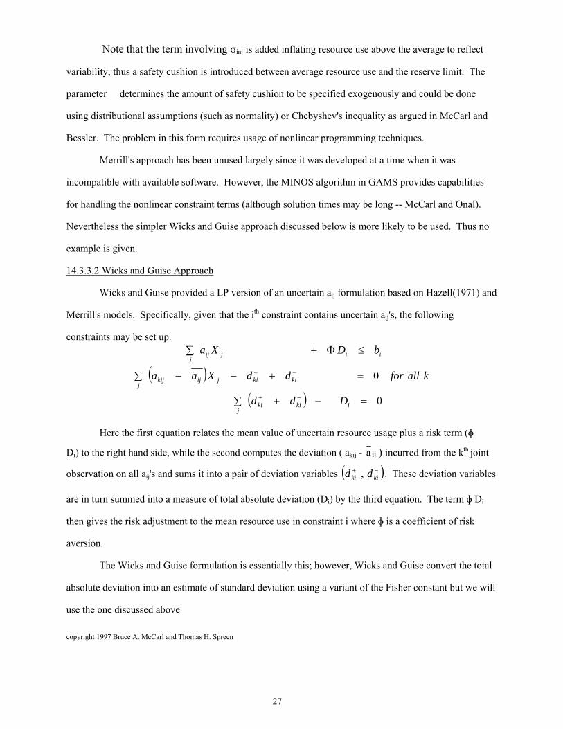
Wicks and Guise provided a LP version of an uncertain aij formulation based on Hazell(1971) and
Merrill's models. Specifically, given that the ith constraint contains uncertain aij's, the following
constraints may be set up.
0
0
ikikij
kikijijkijj
iijijj
Ddd
kallforddXaa
bDXa
Here the first equation relates the mean value of uncertain resource usage plus a risk term (ɸ
Di) to the right hand side, while the second computes the deviation ( akij - ) incurred from the kth joint
observation on all aij's and sums it into a pair of deviation variables kiki dd , . These deviation variables
are in turn summed into a measure of total absolute deviation (Di) by the third equation. The term ɸ Di
then gives the risk adjustment to the mean resource use in constraint i where ɸ is a coefficient of risk
aversion.
The Wicks and Guise formulation is essentially this; however, Wicks and Guise convert the total
absolute deviation into an estimate of standard deviation using a variant of the Fisher constant but we will
use the one discussed above
ija

copyright 1997 Bruce A. McCarl and Thomas H. Spreen
28
ΔD - σ = 0
where Δ = (Π/(2n(n-1))).5 and is the standard error approximation. The general Wicks Guise
formulation is
14.3.3.2.1 Example
Suppose we introduce ingredient uncertainty in the context of the feed problem as discussed in
Chapter V. Suppose one is using three feed ingredients corn, soybeans, and wheat while having to meet
energy and protein requirements. However, suppose that there are four states of nature for energy and
protein nutrient content as given in Table 14.16. Assume that the unit price of corn is 3 cents, soybeans 6
cents, and wheat 4 cents and that the energy requirements are 80% of the unit weight of the feed while the
protein requirement is 50%. In turn, the GAMS formulation of this is called WICKGUIS and a tableau is
given in Table 14.17.
The solution to the Wicks Guise example model are given in Table 14.18. Notice in this table
when the risk aversion parameter is 0 then the model feeds corn and wheat, but as the risk aversion
parameter increases the model first reduces its reliance on corn and increases wheat, but as the risk
aversion parameter gets larger and larger one begins to see soybeans come into the answer. Notice across
these solutions, risk aversion generally increases the average amount of protein with reductions in protein
variability. As the risk aversion parameter increases, the probability of meeting the constraint increases.
Also notice that the shadow price on protein monotonically increases indicating that it is the risky
ingredient driving the model adjustments. Meanwhile average energy decreases, as does energy variation
and the shadow price on energy is zero, indicating there is sufficient energy in all solutions.
14.3.3.2.2 Comments
The reader should note that the deviation variables do not work well unless the constraint
including the risk adjustment is binding. However, if it is not binding, then the uncertainty does not
matter.
The Wicks and Guise formulation has not been widely used. Other than the initial application by
Wicks and Guise the only other application we know of is that of Tice.

copyright 1997 Bruce A. McCarl and Thomas H. Spreen
29
Several other efforts have been made regarding aij uncertainty. The method used in Townsley
and later by Chen (1973) involves bringing a single uncertain constraint into the objective function. The
method used in Rahman and Bender involves developing an over-estimate of variance.
14.3.4 Multiple Sources of Risk
Many problems have C's, A's and b's which are simultaneously uncertain. The formulations
above may be combined to handle such a case. Thus, one could have a E-V model with several
constraints handled via the Wicks Guise and/or chance constrained techniques. There are also techniques
for handling multiple sources of risk under the stochastic programming with recourse topic.
14.4 Sequential Risk-Stochastic Programming with Recourse
Sequential risk arises as part of the risk as time goes on and adaptive decisions are made.
Consider the way that weather and field working time risks are resolved in crop farming. Early on,
planting and harvesting weather are uncertain. After the planting season, the planting decisions have been
made and the planting weather has become known, but harvesting weather is still uncertain. Under such
circumstances a decision maker would adjust to conform to the planting pattern but would still need to
make harvesting decisions in the face of harvest time uncertainty. Thus sequential risk models must
depict adaptive decisions along with fixity of earlier decisions (a decision maker cannot always undo
earlier decisions such as planted acreage). Nonsequential risk, on the other hand, implies that a decision
maker chooses a decision now and finds out about all sources of risk later.
All the models above are nonsequential risk models. Stochastic programming with recourse
(SPR) models are used to depict sequential risk. The first of the models was originally developed as the
"two-stage" LP formulation by Dantzig (1955). Later, Cocks devised a model with N stages, calling it
discrete stochastic programming. Over time, the whole area has been called stochastic programming with
recourse (SPR). We adopt this name.
14.4.1 Two stage SPR formulation
Suppose we set up a two stage SPR formulation. Such formulations contain a probability tree
(Figure 14.3). The nodes of the tree represent decision points. The branches of the tree represent
copyright 1997 Bruce A. McCarl and Thomas H. Spreen
30
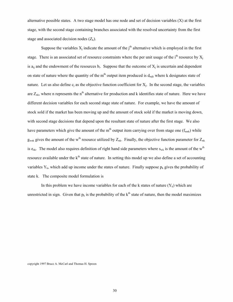
alternative possible states. A two stage model has one node and set of decision variables (X) at the first
stage, with the second stage containing branches associated with the resolved uncertainty from the first
stage and associated decision nodes (Zk).
Suppose the variables Xj indicate the amount of the jth alternative which is employed in the first
stage. There is an associated set of resource constraints where the per unit usage of the ith resource by Xj
is aij and the endowment of the resources bi. Suppose that the outcome of Xj is uncertain and dependent
on state of nature where the quantity of the mth output item produced is dmjk where k designates state of
nature. Let us also define cj as the objective function coefficient for Xj. In the second stage, the variables
are Znk, where n represents the nth alternative for production and k identifies state of nature. Here we have
different decision variables for each second stage state of nature. For example, we have the amount of
stock sold if the market has been moving up and the amount of stock sold if the market is moving down,
with second stage decisions that depend upon the resultant state of nature after the first stage. We also
have parameters which give the amount of the mth output item carrying over from stage one (fmnk) while
gwnk gives the amount of the wth resource utilized by Znk. Finally, the objective function parameter for Znk
is enk. The model also requires definition of right hand side parameters where swk is the amount of the wth
resource available under the kth state of nature. In setting this model up we also define a set of accounting
variables Yk, which add up income under the states of nature. Finally suppose pk gives the probability of
state k. The composite model formulation is
In this problem we have income variables for each of the k states of nature (Yk) which are
unrestricted in sign. Given that pk is the probability of the kth state of nature, then the model maximizes

copyright 1997 Bruce A. McCarl and Thomas H. Spreen
31
knjallforZX
kallforY
kwallforsZg
kmallforZfXd
iallforbXa
kallforZeXcYts
YpMax
nkj
k
wknkwnkn
nkmnkn
jmjkj
ijijj
nknkn
jjl
k
kkk
,,0,
0
,
,0
0..
expected income. Note the income variable under the kth state of nature is equated to the sum of the
nonstochastic income from the first stage variables plus the second stage state of nature dependent profit
contribution. Also note that since Z has taken on the subscript k, the decision variable value will in
general vary by state of nature.
Several points should be noted about this formulation. First, let us note what is risky. In the
second stage the resource endowment (Swk), constraint coefficients (dmjk, fmnk, gwnk) and objective function
parameters (enk) are dependent upon the state. Thus, all types of coefficients (RHS, OBJ and Aij) are
potentially risky and their values depend upon the path through the decision tree.
Second, this model reflects a different uncertainty assumption for X and Z. Note Z is chosen with
knowledge of the stochastic outcomes; however, X is chosen a priori, with it's value fixed regardless of
the stochastic outcomes. Also notice that the first, third, and fourth constraints involve uncertain
parameters and are repeated for each of the states of nature. This problem then has a single X solution
and a Z solution for each state of nature. Thus, adaptive decision making is modeled as the Z variables
are set conditional on the state of nature. Note that irreversabilities and fixity of initial decisions is
modeled. The X variables are fixed across all second stage states of nature, but the Z variables adapt to
the state of nature.
Third, let us examine the linkages between the stages. The coefficients reflect a potentially risky
link between the predecessor (X) and successor (Z) activities through the third constraint. Note the link is
essential since if the activities are not linked, then the problem is not a sequential decision problem.
copyright 1997 Bruce A. McCarl and Thomas H. Spreen
32
These links may involve the weighted sum of a number of predecessor and successor variables (i.e., an
uncertain quantity of lumber harvested via several cutting schemes linked with use in several products).
Also, multiple links may be present (i.e., there may be numerous types of lumber). The subscript m
defines these links. A fourth comment relates to the nature of uncertainty resolution. The formulation
places all uncertainty into the objective function, which maximizes expected income.
14.4.1.1 Example
Let us consider a simple farm planning problem. Suppose we can raise corn and wheat on a 100
acre farm. Suppose per acre planting cost for corn is $100 while wheat costs $60. However, suppose
crop yields, harvest time requirements per unit of yield, harvest time availability and crop prices are
uncertain. The deterministic problem is formulated as in Table 14.20 and file SPREXAM1. Here the
harvest activities are expressed on a per unit yield basis and the income variable equals sales revenue
minus production costs.
The uncertainty in the problem is assumed to fall into two states of nature and is expressed in
Table 14.19. These data give a joint distribution of all the uncertain parameters. Here RHS's, aij's and
objective function coefficient's are uncertain.
Solution of the Table 14.20 LP formulation under each of the states of nature gives two very
different answers. Namely under the first state of nature all acreage is in corn while under the second
state of nature all production is in wheat. These are clearly not robust solutions.
The SPR formulation of this example is given in Table 14.21. This tableau contains one set of
first stage variables (i.e., one set of corn growing and wheat growing activities) coupled with two sets of
second stage variables after the uncertainty is resolved (i.e., there are income, harvest corn, and harvest
wheat variables for both states of nature). Further, there is a single unifying objective function and land
constraint, but two sets of constraints for the states of nature (i.e., two sets of corn and wheat yield
balances, harvesting hour constraints and income constraints). Notice underneath the first stage corn and
wheat production variables, that there are coefficients in both the state of nature dependent constraints
reflecting the different uncertain yields from the first stage (i.e., corn yields 100 bushels under the first
state of nature and 105 under the second; while wheat yields 40 under the first and 38 under the second).
copyright 1997 Bruce A. McCarl and Thomas H. Spreen
33
However, in the second stage resource usage for harvesting is independent. Thus, the 122 hours available
under the first state of nature cannot be utilized by any of the activities under the second state of nature.
Also, the crop prices under the harvest activities vary by state of nature as do the harvest time resource
usages.
The example model then reflects, for example, if one acre of corn is grown that 100 bushels will
be available for harvesting under state of nature one, while 105 will be available under state of nature two.
In the optimum solution there are two harvesting solutions, but one production solution. Thus, we model
irreversibility (i.e., the corn and wheat growing variable levels maximize expected income across the
states of nature, but the harvesting variable levels depend on state of nature).
The SPR solution to this example is shown in Table 14.22. Here the acreage is basically split 50-
50 between corn and wheat, but harvesting differs with almost 4900 bushels of corn harvested under the
first state, where as 5100 bushels of corn are harvested under the second. This shows adaptive decision
making with the harvest decision conditional on state of nature. The model also shows different income
levels by state of nature with $18,145 made under state of nature one and $13,972 under state of nature
two. Furthermore, note that the shadow prices are the marginal values of the resources times the
probability of the state of nature. Thus, wheat is worth $3.00 under the first state of nature but taking into
account that the probability of the first state of nature is 60% we divide the $3.00 by .6 we get the original
$5.00 price. This shows the shadow prices give the contribution to the average objective function. If one
wishes shadow prices relevant to income under a state of nature then one needs to divide by the
appropriate probability.
The income accounting feature also merits discussion. Note that the full cost of growing corn is
accounted for under both the first and second states of nature. However, since income under the first state
of nature is multiplied by .6 and income under the second state of nature is multiplied by .4, then no
double counting is present.
14.4.2 Incorporating Risk Aversion
The two stage model as presented above is risk neutral. This two stage formulation can be altered
to incorporate risk aversion by adding two new sets of constraints and three sets of variables following the

copyright 1997 Bruce A. McCarl and Thomas H. Spreen
34
method used in the unified model above. An EV formulation is
knjallforZddX
kallforYY
kwallforsZg
kmallforZfXd
iallforbXa
kallforZeYXc
kallforddYY
YpYts
ddpYMax
nkkkj
k
wknkwnkn
nkmnkn
jmjkj
ijijj
nknkn
kjjj
kkk
kkk
kkkk
,,0,,,
0,
,
,0
0
0
0..
2
Note that within this formulation the first new constraint that we add simply accounts expected income
into a variable , while the second constraint computes deviations from expected income into new
deviation variables dk+, dk
- which are defined by state of nature. Further, the objective function is
modified so it contains expected income minus a risk aversion parameter times the probabilistically
weighted squared deviations (i.e., variance). This is as an EV model. The model may also be formulated
in the fashion of the unified model discussed earlier to yield either a MOTAD or an E-standard deviation
model.
14.4.2.1 Example
Suppose we use the data from the above Wicks Guise example but also allow decision makers
once they discover the state of nature, to supplement the diet. In this case, suppose the diet supplement to
correct for excess protein deviation costs the firm $0.50 per protein unit while insufficient protein costs
$1.50 per unit. Similarly, suppose excess energy costs $1.00 per unit while insufficient energy costs
$0.10. The resultant SPR tableau, portraying just two of the four states of nature included in the tableau,
is shown in Table 14.23 (This smaller portrayal is only done to preserve readability, the full problem is
solved). Notice we again have the standard structure of an SPR. Namely the corn, soybeans, and wheat
activities are first stage activities, then in the second stage there are positive and negative nutrient
Y
copyright 1997 Bruce A. McCarl and Thomas H. Spreen
35
deviations for each state as well as state dependent objective function and deviation variable accounting.
Notice the average cost row adds the probabilistically weighted sums of the state of nature dependent
variables into average cost while the cost deviation rows compute deviation under a particular state of
nature. In turn, these deviations are weighted by the probability times the risk aversion parameter and are
entered in the objective function. The deviation variables could be treated to form an E-V, MOTAD or E-
Standard error formulation as in the unified model above. An E-standard deviation model will be used
here and is implemented in the GAMS file FEEDSPR. Also note these activities repeat for the second
state of nature and also would for the third and fourth if they were portrayed here.
The risk neutral solution to this problem is given in Table 14.24. Two solution aspects are worth
discussing. First, notice that the first stage solution is to buy .283 pounds of corn, .362 pounds of
soybeans, .355 pounds of wheat at an average cost of 6.7 cents. Cost varies across the states of nature
with cost under the first state equaling 8.1 cents, while under the second state it is 8.3, 5.2 under the third
state and 5.1 under the fourth state. The cost variation arises as the protein and energy shortfall and
excess variables take on different values in order to mitigate nutrient fluctuation.
The model was also solved for risk aversion. The results in Table 14.25 show the solutions from
the example model under varying risk aversion coefficients for a standard deviation implementation.
Table 14.25 gives the changes in corn, soybean, and wheat usage, as well as average income and standard
error of income as the risk aversion parameter is changed for an E-standard deviation formulation as
implemented in the file FEEDSPR. Here the risk aversion parameter was varied from 0.0 up to 0.6. As
risk aversion increases the average cost of the diet increases, but the standard error of the cost of the diet
falls with cost variation between the various states of nature narrowing. Namely under risk neutrality cost
ranges from 5.1 cents to 8.1 cents with a standard error of 1.5 cents, however by the time the risk aversion
parameter is up to .4 the cost varies from only 6.7 to 7.4 cents with a standard error of two tenths of a
cent, at the expense of a 0.4 cent increase in average diet cost. Thus, as risk aversion increases, the model
adopts a plan which stabilizes income across all of the states of nature.
14.4.3 Extending to Multiple Stages
The models above are two stage models with a set of predecessor activities followed by sets of
copyright 1997 Bruce A. McCarl and Thomas H. Spreen
36
successor activities for each state of nature. It is possible to formulate a multiple stage model as done by
Cocks. In such a model however, it is relatively cumbersome to express a general formulation. Thus, we
will express this model only in terms of an example (See Cocks for an N stage formulation and Boisvert
and McCarl for a three stage one). Let us formulate a relatively simple stock model. Suppose that a firm
starts with an initial inventory 100 units of common stock and is trying to maximize average ending
worth. In doing this, suppose that the stock can be sold in one of three time periods. The first one which
is nonstochastic, the second one which is characterized by two states of nature, and the third which is
characterized by two additional states of nature. In describing the states of nature the following data are
relevant. In period one (today) the firm knows the price is $2.00. In period two, the firm is uncertain of
the interest rate between periods and the future price. Assume that under state of nature 1, the interest
rate between period one and two for any stock sold is one percent while it is two percent under the second
state of nature 2. Simultaneously the stock price is $2.20 under the first state of nature and $2.05 under
the second. Going into the third state of nature, the interest rate is conditional on which state of nature
was drawn for the second state. Thus, in the third stage if the first state arose the third stage interest rates
are then either 6% (A) or 4% (B). On the other hand if the second state occurs, the interest rate will either
be 7% (A) or 3% (B). Third stage crop prices are dependent of which of the two third stage states of
nature occur. Under the first state of nature (A) the price is $2.18, while under the second one it is $2.44.
The third stage probabilities are also conditional. Namely, after the first stage one gets state 1 occurring
70% of the time while state 2 occurs 30%of the time. When state 2 results out of stage one then the third
stage probability for state A is 60% and is 40% for state B. On the other hand, these probabilities change
to .7 and .3 if the second state happened out of stage 1.
The resultant formulation of this problem is given in Table 14.26 and file SELLSPR. Here,
again, there is one set of period one variables which refer to either keeping or selling the stock; two sets
of period two variables, which refer again to keep or sell the stock under each second stage state of
nature; and four sets of period three variables for selling the stock and accounting ending net worth under
all the third stage states of nature. Note in the first period, if the stock is kept, it carries over from the first
period to both states of nature in the second stage. Then in the second period the keep activity from the

copyright 1997 Bruce A. McCarl and Thomas H. Spreen
37
first period provides stock that could either be sold or kept on into the third. In turn, if stock is kept in the
second stage, it is held over to both third period states of nature which follow that second period state of
nature. Notice the probabilities of each of the final states are reflected in the average ending worth. The
worth under period three state A following period two state one is multiplied 0.42 which reflects the 70%
probability of period two state one times the 60% conditional probability of period three state A. Also,
notice the prices as they enter the ending worth by state of nature are the sales price in the relevant period
times 1 plus interest earned in the interim periods. Thus, the ending worth of period one sales following
period two state one and period three state A is 2.1412. This reflects the original sales price of $2.00, the
1% interest into the second period and the 6% interest into the third period. The solution to this model is
given in Table 14.27.
14.4.4 Model Discussion
The SPR model is perhaps the most satisfying of the risk models. Conceptually it incorporates all
sources of uncertainty: right hand side, objective function and technical coefficients while allowing
adaptive decisions. However, the formulations suffer from the "curse of dimensionality." Each possible
final state of nature leads to another set of stage two or later activities and large models can result from
relatively simple problems. For example, consider having ten values of two right hand sides which were
independently distributed. This would lead to 100 terminal states or sets of rows. However, such models
can be computationally tractable, since the sparsity and repeated structure tend to make such problems
easier to solve than their size would imply. Thus, one of the things to be cautious about when using this
particular formulation is size. When dealing with such a model, it is often advisable to determine the
critical sources of uncertainty which should be extensively modeled. Uncertainties other than the "most
critical" may be handled with such methods as MOTAD, Wicks and Guise, or chance-constrained as
discussed above. Sources of uncertainty which are not important in the problem may be held at their
expected values (see Tice for an example). Thus, with careful application, this type of model can be quite
useful.
Agricultural economics applications include Yaron and Horowit (1972a); Garoian, et al.; Apland,
et al.(1981); Lambert and McCarl(1989); Leatham and Baker; McCarl and Parandvash; and the early
copyright 1997 Bruce A. McCarl and Thomas H. Spreen
38
papers by Rae (1971a, 1971b). Hansotia; Boisvert and McCarl; and Apland and Kaiser provide literature
reviews.
14.5 General Comments On Modeling Uncertainty
As demonstrated above, there are a number of ways of handling uncertainty when modeling.
Several aspects of these types of models need to be pointed out. First, all the formulations convert the
problems to a deterministic equivalent. Basically, it is assumed that the decision maker is certain of the
risk and reacts to it optimally by discounting the objective function, aij's or right hand sides. Obviously
this means the modeler must assume knowledge of the distribution of risk faced by a decision maker and
the risk aversion coefficient.
The second set of comments regards data. Important parameters within the context of risk models
are the expectation of the coefficient value and its probability distribution around that expectation. The
most common practice for specification of these parameters is to use the historical mean and variance.
This, however, is neither necessary nor always desirable. Fundamentally, the measures that are needed
are the value expected for each uncertain parameter and the perceived probability distribution of
deviations from that expectation (with joint distributions among the various uncertain parameters). The
parameter expectation is not always a historical mean. This is most unrealistic in cases where there has
been a strong historical trend (as pointed out by Chen, 1971). There is a large body of literature dealing
with expectations and/or time series analysis (see Judge for an introduction), and some use of these results
and procedures appears desirable.
Data are most often generated historically; however, observations could be generated by several
other means. For example, observations could be developed from a simulation model (see Dillon, et al.),
from a forecasting equation (see Lambert and McCarl(1989)), or from subjective interrogation of the
decision maker (see Sri Ramaratnam et al.). There are cases where these other methods are more
appropriate than history due to such factors as limited historical data (say, on the price of a new product)
or major structural changes in markets. Naturally, the form in which the data are collected depends on the
particular application involved.
A final comment on data regards their probabilistic nature. Basically when using historically
copyright 1997 Bruce A. McCarl and Thomas H. Spreen
39
based means and variance one is assuming that all observations are equally probable. When this
assumption is invalid, the model is modified so that the value expected is the probabilistically weighted
mean (if desired) and the variance formula includes the consideration of probability (see Anderson, et al.
[pp. 28- 29] for examples). Deviation models must also be adjusted so that the deviations are weighted by
their probability as done in the MOTAD version of the discrete stochastic model in section 14.23.
A third and again independent line of comment relates to the question "should uncertainty be
modeled and if so, how?" Such a concern is paramount to this section. It is obvious from the above that
in modeling uncertainty, data are needed describing the uncertainty, and that modeling uncertainty makes
a model larger and more complex, and therefore harder to interpret, explain, and deal with. It is not the
purpose of these comments to resolve this question, but rather to enter some considerations to the
resolution of this question. First and fundamentally, if a model solution diverges from reality because the
decision maker in reality has somehow considered risk, then it is important to consider risk. This leads to
the subjective judgment on behalf of the modeling team as to whether risk makes a difference. Given that
risk is felt to make a difference, then, how should risk be modeled? In the approaches above, the
formulation model depends upon whether there is conditional decision making and on what is uncertain.
These formulations are not mutually exclusive; rather, it may be desirable to use combinations of these
formulations (see, for example, Wicks and Guise, Tice or Klemme).
Several uncertainty models have not been covered the above discussion. There are more
advanced applications of chance constrained programming such as those found in the books by Sengupta;
Vajda; and Kolbin. Another approach is called "Cautions Suboptimizing" by Day (1979). This approach
bounds the adjustments in variables to a maximum amount in any one year. We also have not covered
Monte Carlo programming as espoused by Anderson, et al., mainly because we do not feel it falls into the
class of programming techniques but rather is a simulation technique.
Finally, it is relevant to discuss how risk should be modeled. There have been arguments
presented in literature (e.g. see, for example, Baker and McCarl or Musser, et al.) that risk model
solutions are biased if the model structure is not adequate before risk modeling is incorporated. Baker
and McCarl argue that one should not include risk until the model structure is fully specified in terms of

copyright 1997 Bruce A. McCarl and Thomas H. Spreen
40
the needed constraints, the time disaggregation of constraints, and activities.

copyright 1997 Bruce A. McCarl and Thomas H. Spreen 41
References Agrawal, R.C. and E.O. Heady. "Application of Game Theory in Agriculture." Journal of Agricultural
Economics. 19(1968):207-218. Anderson, J.R., J.L. Dillon and J.B. Hardaker. Agricultural Decision Analysis. Ames, Iowa: The Iowa
State University Press, 1977. Apland, J.D., B.A. McCarl, and T. Baker. "Crop Residue for Energy Generation: A Prototype
Application to Midwestern USA Grain Prices." Energy in Agriculture. 1(1981):55-78. Apland, J.D., B.A. McCarl, and W.L. Miller. "Risk and the Demand for Supplemental Irrigation: A Case
Study in the Corn Belt." American Journal of Agricultural Economics. 62(1980):142-145. Apland, J.D. and H. Kaiser. "Discrete Stochastic Sequential Programming: A Primer." Staff Papers
Series, Paper P84-8. Institute of Agriculture, Forestry and Home Economics. St. Paul: University of Minnesota, 1984.
Baker, T.G. and B.A. McCarl. "Representing Farm Resource Availability Over Time in Linear Programs:
A Case Study." North Central Journal of Agricultural Economics. 4(1982):59-68. Barry, P. J. (ed.) Risk Management in Agriculture. Ames, Iowa: Iowa State University Press, 1984. Blau, R.A. "Stochastic Programming and Decision Analysis: An Apparent Dilemma." Management
Science. 21(1974):271-276. Boisvert, R. "Available Field Time, Yield Losses and Farm Planning." Canadian Journal of Agricultural
Economics. 24(1976):21-32. Boisvert, R.N. and H. Jensen. "A Method for Planning Under Uncertain Weather Conditions, with
Applications to Corn-Soybean Farming in southern Minnesota." University of Minnesota Agricultural Experiment Station Tech. Bulletin No. 292, 1973.
Boisvert, R.N. and B.A. McCarl. Agricultural Risk Modeling Using Mathematical Programming.
Southern Cooperative Series Bulletin No. 356. Cornell University, New York. July 1990. Brink, L. and B.A. McCarl. "The Adequacy of a Crop Planning Model for Determining Income, Income
Change, and Crop Mix." Canadian Journal of Agricultural Economics. 27(1979):13-15. Brainard, W.C. and R.N. Cooper. "Uncertainty and Diversification in International Trade." Federal
Reserve Institute Studies. 8(1968):257-85. Buccola, S.T. "Minimizing Mean Absolute Deviations to Exactly Solve Expected Utility Problems:
Comment." American Journal of Agricultural Economics. 64(1982):789-91. Bussey, L.E. The Economic Analysis of Industrial Projects. Englewood Cliffs, N.J.: Prentice-Hall, Inc.,
1978.
copyright 1997 Bruce A. McCarl and Thomas H. Spreen 42
Candler, W. and M. Boeljhe. "Use of Linear Programming in Capital Budgeting with Multiple Goals." American Journal of Agricultural Economics. 53(1977):325-330.
Charnes, A. and W.W. Cooper. "Chance Constrained Programming." Management Science. 6(1959):73-
79. Chen, J.T. "Quadratic Programming for Least-Cost Feed Formulations Under Probabilistic Protein
Constraints." American Journal of Agricultural Economics. 55(1973):175-183. Chen, J.T. "A Linear Alternative to Quadratic and semivariance Programming for Form Planning Under
Uncertainty: Comment." American Journal of Agricultural Economics. 53(1971):662-663. Chen, J.T. and C.B. Baker. "Marginal Risk Constraint Linear Program for Activity Analysis." American
Journal of Agricultural Economics. 56(1976):456-465. Cocks, K.D. "Discrete Stochastic Programming." Management Science. 15(1968):72-79. Collender, R.N. and J.A. Chalfant. "An Alternative Approach to Decisions Under Uncertainty Using the
Empirical Moment-Generating Function." American Journal of Agricultural Economics. 68(1986):727-731.
Collender, R.N. and D. Zilberman. "Land Allocation Under Uncertainty for Alternative Technologies
With Stochastic Yield." American Journal of Agricultural Economics. 67(1985):779-793. Curtis, C.E., G.H. Pfieffer, L.L. Lutgen and S.D. Frank. "A Target MOTAD Approach to Marketing
Strategy Selection for Soybeans." North Central Journal of Agricultural Economics. 9(1987)195-206.
Danok, A.B., B.A. McCarl and T.K. White. "Machinery Selection Modeling: Incorporation of Weather
Variability." American Journal of Agricultural Economics. 62(1980):700-08. Dantzig, G. "Linear Programming Under Uncertainty." Management Science. 1(1955):197-206. Day, R. "Cautious Suboptimizing." Risk, Uncertainty and Agricultural Development. Editors J.
Roumasset, J. Boussard and I. Singhe, Agricultural Development Council, New York. Dillon, C.R., J.W. Mjelde and B.A. McCarl. "Biophysical Simulation in Support of Crop Production
Decisions: A Case Study in the Blacklands Region of Texas." Southern Journal of Agricultural Economics. 21(1989):73-86.
Dubman, R.W., L. F. Gunter and B.R. Miller. "Revenue and Cost Uncertainty, Generalized Mean-
Variance and the Linear Complementarity Problem: Comment." American Journal of Agricultural Economics. 61(1989):806-809.
Eisel, L. "Chance Constrained Reservoir Model." Water Resources Research. 8:(1972):339-347. Featherstone, A.M., C.B. Moss, T.G. Baker and P.V. Preckel. "The Theoretical Effects of Farm Policies
on Optimal Leverage and the Probability of Equity Losses." American Journal of Agricultural Economics. 70(1988):572-579.
copyright 1997 Bruce A. McCarl and Thomas H. Spreen 43
Frank, S.D., S.H. Irwin, G.H. Pfeiffer, and C.E. Curtis. "Further Evidence on Soybean Marketing
Strategies: The Role of Options." North Central Journal of Agricultural Economics. 11(1989):213-220.
Freund, R. "The Introduction of Risk into a Programming Model." Econometrica. 21(1956):253-263. Garoian, L., J.R. Conner and C.J. Scifres. "A Discrete Stochastic Programming Model to Estimate
Optimal Burning Schedules on Rangeland." Southern Journal of Agricultural Economics. 19(1987):53-60.
Gebremeskel, T. and C.R. Shumway. "Farm Planning and Calf Marketing Strategies for Risk
Management: An Application of Linear Programming and Statistical Decision Theory." American Journal of Agricultural Economics. 61(1979):363-370.
Hansotia, B.J. "Stochastic Linear Programming With Recourse: A Tutorial." Decision Sciences.
11(1980):151-168. Hazell, P.B.R. "Game Theory - An Extension of Its Application to Farm Planning Under Uncertainty."
Journal of Agricultural Economics. 21(1970):239-252. Hazell, P.B.R. "A Linear Alternative to Quadratic and Semivariance Programming for Farm Planning
under Uncertainty." American Journal of Agricultural Economics. 53(1971):53-62. Hazell, P.B.R. and R.B. How. "Obtaining Acceptable Farm Plans Under Uncertainty." Papers and
Reports 14th International Conference of Agricultural Economists. pp. 338-47. Oxford: Institute for Agricultural Affairs. 1971.
Hazell, P.B.R. and P.L.Scandizzo. "Market Intervention Policies when Production is Risky." American
Journal of Agricultural Economics. 57(1975):641-649. Hazell, P.B.R., R.D. Norton, M. Parthasarthy and C. Pomereda. "The Importance of Risk in Agricultural
Planning Models." The Book of CHAC: Programming Studies for Mexican Agriculture. R.D. Norton and L. Solis (eds.), Baltimore, Md: Johns Hopkins University Press, 1983.
Heady, E.O. and W. Candler. Linear Programming Methods. Ames: Iowa State University Press, 1958. Hogan, A.J., J.G. Morris and H.E. Thompson. "Decision Problems Under Risk and Chance Constrained
Programming: Dilemmas in the Transition." Management Science. 27(1981):716. Hogg, R.V. and A.T. Craig. Introduction to Mathematical Statistics. New York: Macmillan Company,
1970. Jabara, C.L. and R.L. Thompson. "Agricultural Comparative Advantage Under International Price
Uncertainty: The Case of Senegal." American Journal of Agricultural Economics. 62(1980):188-198.
Johnson, D.A. and M.D. Boehlje. "Managing Risk by Coordinating Investment, Marketing and
Production Strategies." Western Journal of Agricultural Economics. 6(1983):155-169.

copyright 1997 Bruce A. McCarl and Thomas H. Spreen 44
Johnson, D. and M.D. Boehlje. "Minimizing Mean Standard Deviations to Exactly Solve Expected
Utility Problems." American Journal of Agricultural Economics. 63(1981):728-29. Judge, G.G. "Estimation and Statistical Inference in Economics." A Survey of American Agricultural
Economics Literature. Vol. 2., L.R. Martin, ed. Minneapolis: University of Minnesota Press, (1977):3-50.
Kawaguchi, T. and Y. Maruyama. "Generalized Constrained Games in Farm Planning." American
Journal of Agricultural Economics. 54(1972):591-702. Kaylen, M.S., R.V. Preckel and E.T. Loehman. "Risk Modeling Via Direct Utility Maximization Using
Numerical Quadrature." American Journal of Agricultural Economics. 69(1987):701-706. Klemme, R.M. "An Economic Analysis of the On-farm Grain Handling Decision Problem."
Unpublished Ph.D. Dissertation, Purdue University, May 1980. Knight, F.H. (1921): Risk, uncertainty and profit. Houghton Mifflin, Boston. Kolbin, V.V. Stochastic Programming. Boston:D. Reidel Publishing Co. 1977. Kroll, Y., H. Levy, and H.M. Markowitz. "Mean-Variance Versus Direct Utility Maximization." Journal
of Finance. 59(1984):47-62. Lambert, D.K. "Calf Retention and Production Decisions Over Time." Western Journal of Agricultural
Economics. 14(1989):9-19. Lambert, D.K. and B.A. McCarl. "Sequential Modeling of White Wheat Marketing Strategies." North
Central Journal of Agricultural Economics. 11(1989):105-115. Lambert, D. and B.A. McCarl. "Risk Modeling Using Direct Solution of Nonlinear Approximations of
the Utility Function." American Journal of Agricultural Economics. 67(1985):846-852. Leatham, D.J. and T.G. Baker. "Farmers' Choice of Fixed and Adjustable Interest Rate Loans."
American Journal of Agricultural Economics. 70(1988):803-812. Levy, H. and H. Markowitz. "Approximating Expected Utility by a Function of Mean and Variance".
American Economic Review. 69(1979):308-317. Lin, W., G.W. Dean and C.V. Moore. "An Empirical Test of Utility vs. Profit Maximization in
Agricultural Production." American Journal of Agricultural Economics. 56(1974):497-508. Loucks, D. "An Evaluation of Some Linear Decision Rules in Chance Constrained Models for Reservoir
Planning and Operation." Water Resource Research. 11(1975):777-82. Low, A.R.C. "Decision Making Under Uncertainty: A Linear Programming Model of Peasant Farmer
Behavior." Journal of Agricultural Economics. 25(1974):311-322. Maji, C. and E. Heady. "Intertemporal Allocation of Irrigation Water in the Mayurakshi Project (India):

copyright 1997 Bruce A. McCarl and Thomas H. Spreen 45
An Application of Chance Constrained Linear Programming." Water Resources Research. 14(1978):190-205.
Mapp, H.P. Jr., M.L. Hardin, O.L. Walker and T. Persand. "Analysis of Risk Management Strategies for
Agricultural Producers." American Journal of Agricultural Economics. 61(1979):1071-1077. Markowitz, H.M. Portfolio Selection: Efficient Diversification of Investments. New York: John Wiley
and Sons, Inc., 1959. Maruyama, Y. "A Truncated Maximum Approach to Farm Planning Under Uncertainty with Discrete
Probability Distributions." American Journal of Agricultural Economics. 54(1972):192-200. McCamley, F. and J.B. Kliebenstein. "Describing and Identifying the Complete Set of Target MOTAD
Solutions." American Journal of Agricultural Economics. 69(1987):669-76. McCarl, B.A. and D. Bessler. "Estimating an Upper Bound on the Pratt Risk Aversion Coefficient When
the Utility Function is Unknown." Australian Journal of Agricultural Economics. 33(1989):56-63.
McCarl, B.A., W. Candler, D. Doster, and P. Robbins. "Experiences with Farmer Oriented Linear
Programming for Crop Farming." Canadian Journal of Agricultural Economics. 24(1977):17-30. McCarl, B.A. and H. Onal. "Linear Approximation of Using MOTAD and Separable Programming:
Should It Be Done." American Journal of Agricultural Economics. 71(1989):158-165. McCarl, B.A. and G.H. Parandvash. "Irrigation Develop Versus Hydroelectric Generation: Can
Interruptable Irrigation Play a Role." Western Journal of Agricultural Economics. 13(1988):267-276.
McCarl, B.A. and T. Tice. "Should Quadratic Programming Problems be Approximated?" American
Journal of Agricultural Economics. 64(1982):585-589. McFarquhar, A.M.M. "Rational Decision Making and Risk in Farm Planning - An Application of
Quadratic Programming in British Arable Farming." Journal of Agricultural Economics. 14(1961):552-563.
McInerney, J.P. "Maximum Programming - An Approach to Farm Planning Under Uncertainty." Journal
of Agricultural Economics. 18(1967):279-290. McInerney, J.P. "Linear Programming and Game Theory Models - Some Extensions." Journal of
Agricultural Economics. 20(1969):269-278. Merrill, W.C. "Alternative Programming Models Involving Uncertainty." Journal of Farm Economics.
47(1965):595-610. Meyer, J. "Two-Moment Decision Models and Expected Utility Maximization." American Economic
Review. 77(1987):421-430. Moffit, L.J., T.M. Burrows, J.L. Baritelle and V. Sevacherian. "Risk Evaluation of Early Termination for
copyright 1997 Bruce A. McCarl and Thomas H. Spreen 46
pest Control in Cotton." Western Journal of Agricultural Economics. 9(1984):145-151. Musser, W.N., B.A. McCarl and G.S. Smith. "An Investigation of the Relationship Between Constraint
Omission and Risk Aversion in Firm Risk Programming Models." Southern Journal of Agricultural Economics. 18(1986):147-154.
Nieuwoudt, W.L., J.B. Bullock and G.A. Mathia. "An Economic Evaluation of Alternative Peanut
Policies." American Journal of Agricultural Economics. 58(1976):485-495. Paris, Q. "Revenue and Cost Uncertainty, Generalized Mean-Variance, and the Linear Complementarity
Problem." American Journal of Agricultural Economics. 61(1979):268-275. Paris, Q. "Revenue and Cost Uncertainty, Generalized Mean-Variance and the Linear Complementarity
Problem: Reply." American Journal of Agricultural Economics. 61(1989):810-812. Pfaffenberger, R.C. and D.A. Walker. Mathematical Programming for Economics and Business. Ames:
Iowa State University Press, 1976. Pomareda, C. and O. Samayoa. "Area and Yield Response to Price Policy: A Case Study in Guatemala,
C.A." American Journal of Agricultural Economics. 61(1979):683-86. Preckel, P.V., A.M. Featherstone, and T.G. Baker. "Interpreting Dual Variables for Optimization with
Nonmonetary Objectives." American Journal of Agricultural Economics. 69(1987):849-851. Rae, A.N. "Stochastic Programming, Utility, and Sequential Decision Problems in Farm Management."
American Journal of Agricultural Economics. 53(1971a):448-60. Rae, A.N. "An Empirical Application and Evaluation of Discrete Stochastic Programming in Farm
Management." American Journal of Agricultural Economics. 53(1971b):625-38. Rahman, S.A. and F.E. Bender. "Linear Programming Approximation of Least-Cost Feed Mixes with
Probability Restrictions." American Journal of Agricultural Economics. 53(1971):612-18. Reid, D.W. and B.V. Tew. "An Evaluation of Expected Value and Expected Value-Variance Criteria in
Achieving Risk Efficiency in Crop Selection." Northeastern Journal of Agricultural and Resource Economics. 16(1987):93-101.
Robinson, L.J. and J.R. Brake. "Application of Portfolio Theory to Farmer and Lender Behavior."
American Journal of Agricultural Economics. 61(1979):159-164. Roy, A.D. "Safety-First and the Holding of Assets." Econometrica. 20(1952):431-449. Schurle, B.W. and B.L. Erven. "Sensitivity of Efficient Frontiers Developed for Farm Enterprise Choice
Decisions." American Journal of Agricultural Economics. 61(1979):506-511. Sengupta, J.K. Stochastic Programming: Methods and Applications. New York: American Elsevier
Publishing Company, Inc. 1972. Sharpe, W. "A Linear Programming Algorithm for Mutual Fund Portfolio Selection." Management
copyright 1997 Bruce A. McCarl and Thomas H. Spreen 47
Science. 14(1967):499-510. Simmons, R.L. and C. Pomareda. "Equilibrium Quantity and Timing of Mexican Vegetable Exports."
American Journal of Agricultural Economics. 57(1975):472-479. Sri Ramaratnam, S., M.E. Rister, D.A. Bessler, and James Novak. "Risk Attitudes and Farm/Producer
Attributes: A Case Study of Texas Coastal Bend Grain Sorghum Producers." Southern Journal of Agricultural Economics . 18(1986):85-95.
Stovall, J. "Income Variation and Selection of Enterprises." Journal of Farm Economics.
48(1966):1575-1579. Tauer, L. "Target MOTAD." American Journal of Agricultural Economics. 65(1983):606-610. Thomas, W., L. Blakeslee, L. Rogers and N. Whittlesey. "Separable Programming for Considering Risk
in Farm Planning." American Journal of Agricultural Economics. 54(1972):260-266. Thomson, K. and P.B.R. Hazell. "Reliability of Using the Mean Absolute Deviation to Derive Efficient
E-V farm Plans." American Journal of Agricultural Economics. 54(1972):503-506. Tice, T.F. "An Investigation of Nitrogen Application Under Uncertainty." Unpublished Ph.D.
Dissertation, Purdue University, August 1979. Tobin, J. "Liquidity Preference as Behavior toward Risk." Review of Economic Studies. 25(1958):65-
86. Townsley, R. "Derivation of Optimal Livestock Rations Using Quadratic Programming." Journal of
Agricultural Economics. 19(1968):347-354. Tsiang, S. "The Rationale of the Mean-Standard Deviation Analysis, Skewness, Preference and the
Demand for Money." American Economic Review. 62(1972):354-371. Tsiang, S. "The Rationale of the Mean-Standard Deviation Analysis: Reply and Errate for Original
Article." American Economic Review. 64(1974):442-450. Vajda, S. Probabilistic Programming. New York: Academic Press, 1972. von Neumann, J. and O. Morgenstern. Theory of Games and Economic Behavior. Princeton, N.J.:
Princeton University Press, 1947. Wagner, H.M. Principles of Operations Research. Englewood Cliffs, N.J.: Prentice Hall, Inc. 1975. Weins, J.A. "Peasant Risk Aversion and Allocative Behavior: A Quadratic Programming Experiment."
American Journal of Agricultural Economics. 58(1976):629-635. Wicks, J.A. and J.W.B. Guise. "An Alternative Solution to Linear programming Problems with
Stochastic Input-Output Coefficients." Australian Journal of Agricultural Economics.

copyright 1997 Bruce A. McCarl and Thomas H. Spreen 48
22(1978):22-40. Yaron, D., and V. Horowitz. "A Sequential Programming Model of Growth and Capital Accumulation of
a Farm Under Uncertainty." American Journal of Agricultural Economics. 54(1972):441-451. Yassour, J.D., D. Zilberman and G.C. Rausser. "Optional Choices Among Alternative Technologies with
Stochastic Yield." American Journal of Agricultural Economics. 63(1981):718-723. Yitzhaki, S. "Stochastic Dominance, Mean Variance and Gini's Mean Difference." American Economic
Review. 72(1982):178-185. Young, D.L. "Evaluating Procedures for Computing Objective Risk from Historical Time Series." Paper
presented at Annual Meeting of Western Regional Research Project W-149, Tucson, Arizona. January 16-18, 1980.
Zimet, D.J. and T.H. Spreen. "A Target MOTAD Analysis of a Crop and Livestock Farm in Jefferson
County, Florida." Southern Journal of Agricultural Economics. 18(1986):175-185.
Table 14.1. Data for E-V Example -- Returns by Stock and Event
----Stock Returns by Stock and Event----
Stock1 Stock2 Stock3 Stock4
Event1 7 6 8 5
Event2 8 4 16 6
Event3 4 8 14 6
Event4 5 9 -2 7
Event5 6 7 13 6
Event6 3 10 11 5
Event7 2 12 -2 6
Event8 5 4 18 6
Event9 4 7 12 5
Event10 3 9 -5 6
Stock1 Stock2 Stock3 Stock4
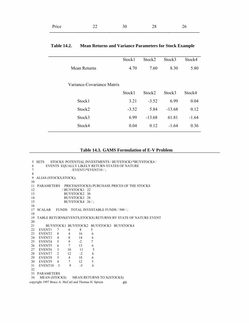
copyright 1997 Bruce A. McCarl and Thomas H. Spreen 49
Price 22 30 28 26
Table 14.2. Mean Returns and Variance Parameters for Stock Example
Stock1 Stock2 Stock3 Stock4
Mean Returns 4.70 7.60 8.30 5.80
Variance-Covariance Matrix
Stock1 Stock2 Stock3 Stock4
Stock1 3.21 -3.52 6.99 0.04
Stock2 -3.52 5.84 -13.68 0.12
Stock3 6.99 -13.68 61.81 -1.64
Stock4 0.04 0.12 -1.64 0.36
Table 14.3. GAMS Formulation of E-V Problem
5 SETS STOCKS POTENTIAL INVESTMENTS / BUYSTOCK1*BUYSTOCK4 / 6 EVENTS EQUALLY LIKELY RETURN STATES OF NATURE 7 /EVENT1*EVENT10 / ; 8 9 ALIAS (STOCKS,STOCK); 10 11 PARAMETERS PRICES(STOCKS) PURCHASE PRICES OF THE STOCKS 12 / BUYSTOCK1 22 13 BUYSTOCK2 30 14 BUYSTOCK3 28 15 BUYSTOCK4 26 / ; 16 17 SCALAR FUNDS TOTAL INVESTABLE FUNDS / 500 / ; 18 19 TABLE RETURNS(EVENTS,STOCKS) RETURNS BY STATE OF NATURE EVENT 20 21 BUYSTOCK1 BUYSTOCK2 BUYSTOCK3 BUYSTOCK4 22 EVENT1 7 6 8 5 23 EVENT2 8 4 16 6 24 EVENT3 4 8 14 6 25 EVENT4 5 9 -2 7 26 EVENT5 6 7 13 6 27 EVENT6 3 10 11 5 28 EVENT7 2 12 -2 6 29 EVENT8 5 4 18 6 30 EVENT9 4 7 12 5 31 EVENT10 3 9 -5 6 32 33 PARAMETERS 34 MEAN (STOCKS) MEAN RETURNS TO X(STOCKS)

copyright 1997 Bruce A. McCarl and Thomas H. Spreen 50
35 COVAR(STOCK,STOCKS) VARIANCE COVARIANCE MATRIX; 36 37 MEAN(STOCKS) = SUM(EVENTS , RETURNS(EVENTS,STOCKS) / CARD(EVENTS) ); 38 COVAR(STOCK,STOCKS) 39 = SUM (EVENTS ,(RETURNS(EVENTS,STOCKS) - MEAN(STOCKS)) 40 *(RETURNS(EVENTS,STOCK)- MEAN(STOCK)))/CARD(EVENTS); 41 42 DISPLAY MEAN , COVAR ; 43 44 SCALAR RAP RISK AVERSION PARAMETER / 0.0 / ; 45 46 POSITIVE VARIABLES INVEST(STOCKS) MONEY INVESTED IN EACH STOCK 47 48 VARIABLE OBJ NUMBER TO BE MAXIMIZED ; 49 50 EQUATIONS OBJJ OBJECTIVE FUNCTION 51 INVESTAV INVESTMENT FUNDS AVAILABLE 52 ; 53 54 OBJJ.. 55 OBJ =E= SUM(STOCKS, MEAN(STOCKS) * INVEST(STOCKS)) 56 - RAP*(SUM(STOCK, SUM(STOCKS, 57 INVEST(STOCK)* COVAR(STOCK,STOCKS) * INVEST(STOCKS)))); 58 59 INVESTAV.. SUM(STOCKS, PRICES(STOCKS) * INVEST(STOCKS)) =L= FUNDS ; 60 61 MODEL EVPORTFOL /ALL/ ; 62 63 SOLVE EVPORTFOL USING NLP MAXIMIZING OBJ ; 64 65 SCALER VAR THE VARIANCE ; 66 VAR = SUM(STOCK, SUM(STOCKS, 67 INVEST.L(STOCK)* COVAR(STOCK,STOCKS) * INVEST.L(STOCKS))) ;
68 DISPLAY VAR ; 69
70 SET RAPS RISK AVERSION PARAMETERS /R0*R25/ 71 72 PARAMETER RISKAVER(RAPS) RISK AVERSION COEFICIENTS 73 /R0 0.00000, R1 0.00025, R2 0.00050, R3 0.00075, 74 R4 0.00100, R5 0.00150, R6 0.00200, R7 0.00300, 75 R8 0.00500, R9 0.01000, R10 0.01100, R11 0.01250, 76 R12 0.01500, R13 0.02500, R14 0.05000, R15 0.10000, 77 R16 0.30000, R17 0.50000, R18 1.00000, R19 2.50000, 78 R20 5.00000, R21 10.0000, R22 15. , R23 20. 79 R24 40. , R25 80./ 80 81 PARAMETER OUTPUT(*,RAPS) RESULTS FROM MODEL RUNS WITH VARYING RAP 82 83 OPTION SOLPRINT = OFF; 84 85 LOOP (RAPS,RAP=RISKAVER(RAPS); 86 SOLVE EVPORTFOL USING NLP MAXIMIZING OBJ ; 87 VAR = SUM(STOCK, SUM(STOCKS, 88 INVEST.L(STOCK)* COVAR(STOCK,STOCKS) * INVEST.L(STOCKS))) ; 89 OUTPUT("OBJ",RAPS)=OBJ.L; 90 OUTPUT("RAP",RAPS)=RAP; 91 OUTPUT(STOCKS,RAPS)=INVEST.L(STOCKS); 92 OUTPUT("MEAN",RAPS)=SUM(STOCKS, MEAN(STOCKS)*INVEST.L(STOCKS)); 93 OUTPUT("VAR",RAPS) = VAR; 94 OUTPUT("STD",RAPS)=SQRT(VAR); 95 OUTPUT("SHADPRICE",RAPS)=INVESTAV.M; 96 OUTPUT("IDLE",RAPS)=FUNDS-INVESTAV.L 97 ); 98 DISPLAY OUTPUT;
copyright 1997 Bruce A. McCarl and Thomas H. Spreen 51
Table 14.4. E-V Example Solutions for Alternative Risk Aversion Parameters

copyright 1997 Bruce A. McCarl and Thomas H. Spreen 52
RAP 0 0.00025 0.0005 0.00075 0.001 BUYSTOCK2 1.263 5.324 7.355 BUYSTOCK3 17.857 17.857 16.504 12.152 9.977 OBJ 148.214 143.287 138.444 135.688 134.245 MEAN 148.214 148.214 146.581 141.331 138.705 VAR 19709.821 19709.821 16274.764 7523.441 4460.478 STD 140.392 140.392 127.573 86.738 66.787 SHADPRICE 0.296 0.277 0.261 0.260 0.260 RAP 0.0015 0.002 0.003 0.005 0.010 BUYSTOCK2 9.386 10.401 11.416 12.229 12.838 BUYSTOCK3 7.801 6.713 5.625 4.755 4.102 OBJ 132.671 131.753 130.575 129.005 125.999 MEAN 136.080 134.767 133.454 132.404 131.617 VAR 2272.647 1506.907 959.949 679.907 561.764 STD 47.672 38.819 30.983 26.075 23.702 SHADPRICE 0.259 0.257 0.255 0.251 0.241 RAP 0.011 0.012 0.015 0.025 0.050 BUYSTOCK1 1.273 4.372 4.405 BUYSTOCK2 12.893 12.960 12.420 11.070 8.188 BUYSTOCK3 4.043 3.972 3.550 2.561 1.753 BUYSTOCK4 4.168 OBJ 125.441 124.614 123.380 120.375 116.805 MEAN 131.545 131.459 129.839 125.939 121.656 VAR 554.929 547.587 430.560 222.576 97.026 STD 23.557 23.401 20.750 14.919 9.850 SHADPRICE 0.239 0.236 0.234 0.230 0.224 RAP 0.100 0.300 0.500 1.000 2.500 BUYSTOCK1 4.105 3.905 3.865 3.835 1.777 BUYSTOCK2 6.488 5.354 5.128 4.958 2.289 BUYSTOCK3 1.340 1.064 1.009 0.968 0.446 BUYSTOCK4 6.829 8.602 8.957 9.223 4.296 OBJ 113.118 102.254 92.010 66.674 27.185 MEAN 119.327 117.774 117.463 117.230 54.370 VAR 62.086 51.734 50.905 50.556 10.874 STD 7.879 7.193 7.135 7.110 3.298 SHADPRICE 0.214 0.173 0.133 0.032 0 IDLE FUNDS 268.044
Notes: RAP is the risk aversion parameter (ɸ) value Stocki gives the amount invested in stocki Obj gives the objective function value Mean gives expected income Var gives the variance of income STD gives the standard deviation of income Shadprice gives the shadow price on the capital available constraint

copyright 1997 Bruce A. McCarl and Thomas H. Spreen 53
Table 14.5. Deviations from the Mean for Portfolio Example
Stock1 Stock2 Stock3 Stock4
Event1 2.3 -1.6 -0.3 -0.8
Event2 3.3 -3.6 7.7 0.2
Event3 -0.7 0.4 5.7 0.2
Event4 0.3 1.4 -10.3 1.2
Event5 1.3 -0.6 4.7 0.2
Event6 -1.7 2.4 2.7 -0.8
Event7 -2.7 4.4 -10.3 0.2
Event8 0.3 -3.6 9.7 0.2
Event9 -0.7 -0.6 3.7 -0.8
Event10 -1.7 1.4 -13.3 0.2

copyright 1997 Bruce A. McCarl and Thomas H. Spreen 54
Table 14.6. Example MOTAD Model Formulation
0σTNDΔ
0TNDd
0dX0.200X13.300X1.400X1.700
0dX0.800X3.700X0.600X0.700
0dX0.200X9.700X3.600X0.300
0dX0.200X10.300X4.400X2.700
0dX0.800X2.700X2.400X1.700
0dX0.200X4.700X0.600X1.300
0dX1.200X10.300X1.400X0.300
0dX0.200X5.700X0.400X0.700
0dX0.200X7.700X3.600X3.300
0dX0.800X0.300X1.600X2.300
500X26X28X30X22s.t.
σγX5.80X8.30X7.60X4.70Max
kk
104321
94321
84321
74321
64321
54321
44321
34321
24321
14321
4321
4321
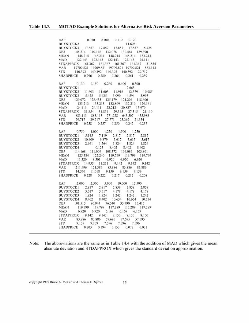
copyright 1997 Bruce A. McCarl and Thomas H. Spreen 55
Table 14.7. MOTAD Example Solutions for Alternative Risk Aversion Parameters
RAP 0.050 0.100 0.110 0.120 BUYSTOCK2 11.603 BUYSTOCK3 17.857 17.857 17.857 17.857 5.425 OBJ 148.214 140.146 132.078 130.464 129.390 MEAN 148.214 148.214 148.214 148.214 133.213 MAD 122.143 122.143 122.143 122.143 24.111 STDAPPROX 161.367 161.367 161.367 161.367 31.854 VAR 19709.821 19709.821 19709.821 19709.821 883.113 STD 140.392 140.392 140.392 140.392 29.717 SHADPRICE 0.296 0.280 0.264 0.261 0.259 RAP 0.130 0.150 0.260 0.400 0.500 BUYSTOCK1 2.663 BUYSTOCK2 11.603 11.603 11.916 12.379 10.985 BUYSTOCK3 5.425 5.425 5.090 4.594 3.995 OBJ 129.072 128.435 125.179 121.204 118.606 MEAN 133.213 133.213 132.809 132.210 129.161 MAD 24.111 24.111 22.212 20.827 15.979 STDAPPROX 31.854 31.854 29.345 27.515 21.110 VAR 883.113 883.113 771.228 643.507 455.983 STD 29.717 29.717 27.771 25.367 21.354 SHADPRICE 0.258 0.257 0.250 0.242 0.237 RAP 0.750 1.000 1.250 1.500 1.750 BUYSTOCK1 5.145 7.119 2.817 2.817 2.817 BUYSTOCK2 10.409 9.879 5.617 5.617 5.617 BUYSTOCK3 2.661 1.564 1.824 1.824 1.824 BUYSTOCK4 0.123 8.402 8.402 8.402 OBJ 114.168 111.009 108.372 106.086 103.801 MEAN 125.384 122.240 119.799 119.799 119.799 MAD 11.320 8.501 6.920 6.920 6.920 STDAPPROX 14.955 11.231 9.142 9.142 9.142 VAR 211.996 121.386 83.886 83.886 83.886 STD 14.560 11.018 9.159 9.159 9.159 SHADPRICE 0.228 0.222 0.217 0.212 0.208 RAP 2.000 2.500 5.000 10.000 12.500 BUYSTOCK1 2.817 2.817 2.858 2.858 2.858 BUYSTOCK2 5.617 5.617 4.178 4.178 4.178 BUYSTOCK3 1.824 1.824 1.242 1.242 1.242 BUYSTOCK4 8.402 8.402 10.654 10.654 10.654 OBJ 101.515 96.944 76.540 35.790 15.415 MEAN 119.799 119.799 117.289 117.289 117.289 MAD 6.920 6.920 6.169 6.169 6.169 STDAPPROX 9.142 9.142 8.150 8.150 8.150 VAR 83.886 83.886 57.695 57.695 57.695 STD 9.159 9.159 7.596 7.596 7.596 SHADPRICE 0.203 0.194 0.153 0.072 0.031
Note: The abbreviations are the same as in Table 14.4 with the addition of MAD which gives the mean
absolute deviation and STDAPPROX which gives the standard deviation approximation.
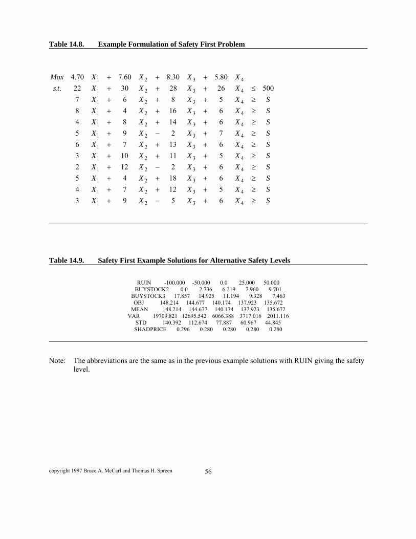
copyright 1997 Bruce A. McCarl and Thomas H. Spreen 56
Table 14.8. Example Formulation of Safety First Problem
Table 14.9. Safety First Example Solutions for Alternative Safety Levels
RUIN -100.000 -50.000 0.0 25.000 50.000 BUYSTOCK2 0.0 2.736 6.219 7.960 9.701
BUYSTOCK3 17.857 14.925 11.194 9.328 7.463 OBJ 148.214 144.677 140.174 137.923 135.672
MEAN 148.214 144.677 140.174 137.923 135.672 VAR 19709.821 12695.542 6066.388 3717.016 2011.116
STD 140.392 112.674 77.887 60.967 44.845 SHADPRICE 0.296 0.280 0.280 0.280 0.280
Note: The abbreviations are the same as in the previous example solutions with RUIN giving the safety level.
SXXXX
SXXXX
SXXXX
SXXXX
SXXXX
SXXXX
SXXXX
SXXXX
SXXXX
SXXXX
XXXXts
XXXXMax
4321
4321
4321
4321
4321
4321
4321
4321
4321
4321
4321
4321
6593
51274
61845
62122
511103
61376
7295
61484
61648
5867
50026283022..
80.530.860.770.4

copyright 1997 Bruce A. McCarl and Thomas H. Spreen 57
Table 14.10. Example Formulation of Target MOTAD Problem
λDev
TDevX6X5XX3
TDevX5X12XX4
TDevX6X18XX5
TDevX6X2XX2
TDevX5X11XX3
TDevX6X13XX6
TDevX7X2XX5
TDevX6X14XX4
TDevX6X16XX8
TDevX5X8XX7
500X26X28XX22s.t.
X5.80X8.30X7.60X4.70Max
kk
104321
94321
84321
74321
64321
54321
44321
34321
24321
14321
4321
4321
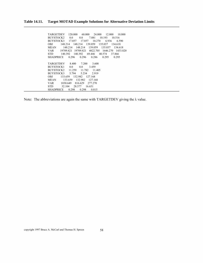
copyright 1997 Bruce A. McCarl and Thomas H. Spreen 58
Table 14.11. Target MOTAD Example Solutions for Alternative Deviation Limits
TARGETDEV 120.000 60.000 24.000 12.000 10.800 BUYSTOCK2 0.0 0.0 7.081 10.193 10.516 BUYSTOCK3 17.857 17.857 10.270 6.936 6.590 OBJ 148.214 148.214 139.059 135.037 134.618 MEAN 148.214 148.214 139.059 135.037 134.618 VAR 19709.821 19709.821 4822.705 1646.270 1433.820 STD 140.392 140.392 69.446 40.574 37.866 SHADPRICE 0.296 0.296 0.286 0.295 0.295 TARGETDEV 8.400 7.200 3.600 BUYSTOCK1 0.0 0.0 3.459 BUYSTOCK2 11.259 11.782 11.405 BUYSTOCK3 5.794 5.234 2.919 OBJ 133.659 132.982 127.168 MEAN 133.659 132.982 127.168 VAR 1030.649 816.629 277.270 STD 32.104 28.577 16.651 SHADPRICE 0.298 0.298 0.815
Note: The abbreviations are again the same with TARGETDEV giving the λ value.

copyright 1997 Bruce A. McCarl and Thomas H. Spreen 59
Table 14.12. Example Formulation of DEMP Problem
100X6X5X9X3W
100X5X12X7X4W
100X6X18X4X5W
100X6X2X12X2W
100X5X11X10X3W
100X6X13X7X6W
100X7X2X9X5W
100X6X14X8X4W
100X6X16X4X8W
100X5X8X6X7W
500X26X28X30X22s.t.
)(WMax
432110
43219
43218
43217
43216
43215
43214
43213
43212
43211
4321
k
powerk

copyright 1997 Bruce A. McCarl and Thomas H. Spreen 60
Table 14.13. DEMP Example Solutions for Alternative Utility Function Exponents
POWER 0.950 0.900 0.750 0.500 0.400 BUYSTOCK2 4.560 8.563 9.344 BUYSTOCK3 17.857 17.857 12.972 8.683 7.846 OBJ 186.473 140.169 60.363 15.282 8.848 MEAN 248.214 248.214 242.319 237.144 236.134 VAR 19709.821 19709.821 8903.295 3054.034 2309.233 STD 140.392 140.392 94.357 55.263 48.054 SHADPRICE 0.287 0.277 0.269 0.266 0.265 POWER 0.300 0.200 0.100 0.050 0.030 BUYSTOCK2 9.919 10.358 10.705 10.852 10.907 BUYSTOCK3 7.230 6.759 6.388 6.230 6.171 OBJ 5.127 2.972 1.724 1.313 1.177 MEAN 235.390 234.822 234.374 234.184 234.113 VAR 1843.171 1534.736 1320.345 1236.951 1207.076 STD 42.932 39.176 36.337 35.170 34.743 SHADPRICE 0.264 0.264 0.263 0.263 0.263 POWER 0.020 0.010 0.001 0.0001 BUYSTOCK2 10.934 10.960 10.960 10.960 BUYSTOCK3 6.143 6.115 6.115 6.115 OBJ 1.115 1.056 1.005 1.001 MEAN 234.079 234.045 234.045 234.045 VAR 1192.805 1178.961 1178.961 1178.961 STD 34.537 34.336 34.336 34.336 SHADPRICE 0.263 0.263 0.263 0
Note: The abbreviations are again the same with POWER giving the exponent used.
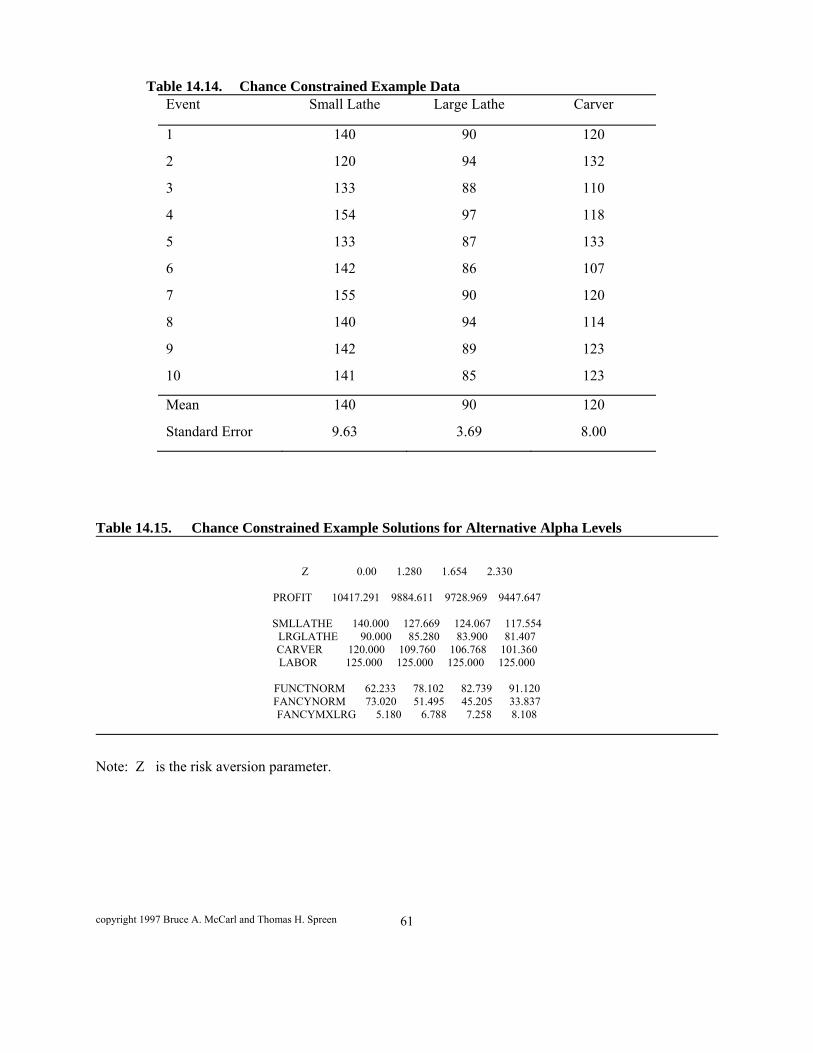
copyright 1997 Bruce A. McCarl and Thomas H. Spreen 61
Table 14.14. Chance Constrained Example Data Event Small Lathe Large Lathe Carver
1 140 90 120
2 120 94 132
3 133 88 110
4 154 97 118
5 133 87 133
6 142 86 107
7 155 90 120
8 140 94 114
9 142 89 123
10 141 85 123
Mean 140 90 120
Standard Error 9.63 3.69 8.00
Table 14.15. Chance Constrained Example Solutions for Alternative Alpha Levels
Z� 0.00 1.280 1.654 2.330
PROFIT 10417.291 9884.611 9728.969 9447.647
SMLLATHE 140.000 127.669 124.067 117.554 LRGLATHE 90.000 85.280 83.900 81.407 CARVER 120.000 109.760 106.768 101.360 LABOR 125.000 125.000 125.000 125.000
FUNCTNORM 62.233 78.102 82.739 91.120 FANCYNORM 73.020 51.495 45.205 33.837 FANCYMXLRG 5.180 6.788 7.258 8.108
Note: Z� is the risk aversion parameter.
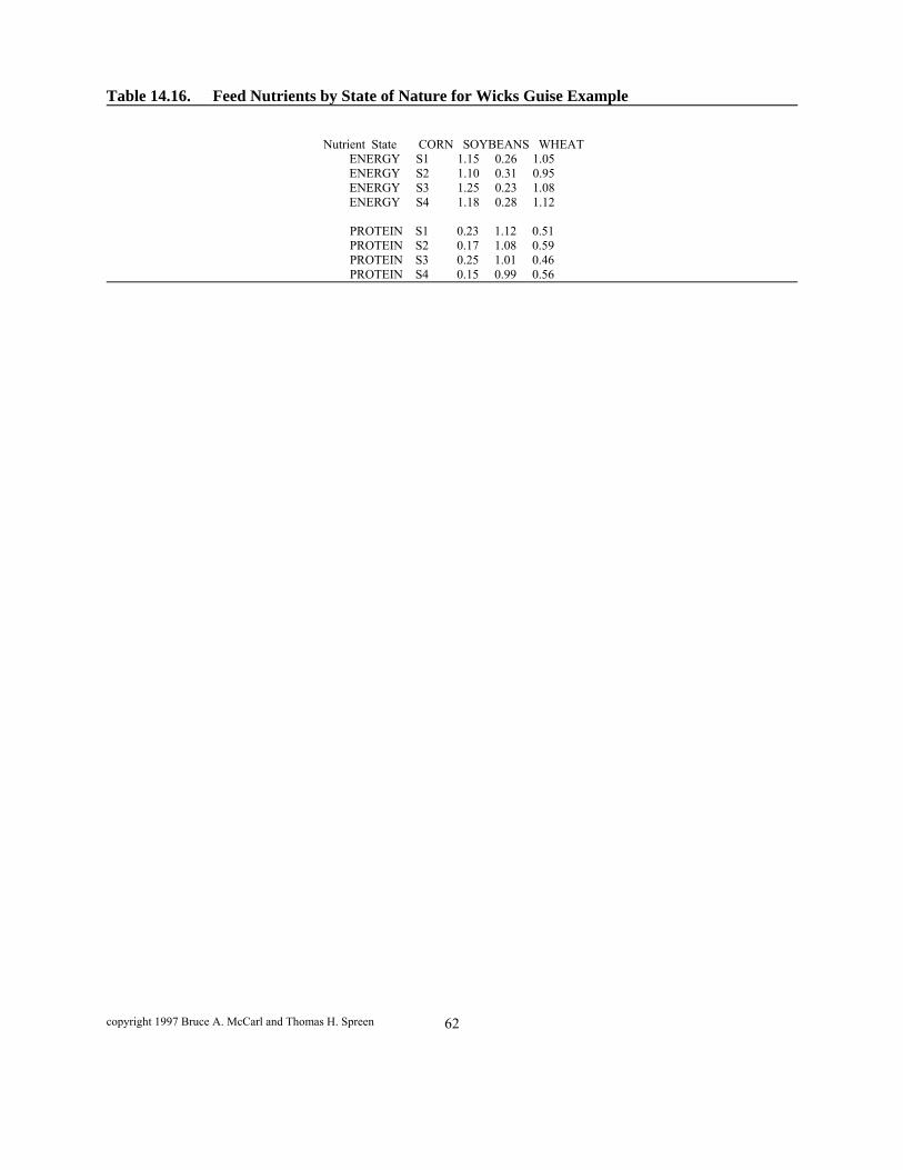
copyright 1997 Bruce A. McCarl and Thomas H. Spreen 62
Table 14.16. Feed Nutrients by State of Nature for Wicks Guise Example
Nutrient State CORN SOYBEANS WHEAT ENERGY S1 1.15 0.26 1.05 ENERGY S2 1.10 0.31 0.95 ENERGY S3 1.25 0.23 1.08 ENERGY S4 1.18 0.28 1.12
PROTEIN S1 0.23 1.12 0.51 PROTEIN S2 0.17 1.08 0.59 PROTEIN S3 0.25 1.01 0.46 PROTEIN S4 0.15 0.99 0.56

copyright 1997 Bruce A. McCarl and Thomas H. Spreen 63
Table 14.17. Wicks Guise Example
Note: EnDev is the energy deviation EnMAD is the energy mean absolute deviation Enσ is the energy standard deviation approximations PrDev is the protein deviation PrMAD is the protein mean absolute deviation Prσ is the protein standard deviation approximation
01ΔσProtein
01)/4d(dProteinMAD
0dd0.070.010.01Proteins4
0dd0.030.040.08Proteins3
0dd0.100.040.07Proteins2
0dd0.000.010.02Proteins101ΔσEnergy
01)/4d(d
0dd0.070.010.01
0dd0.030.040.08
0dd0.100.040.07
0dd0.000.010.020.50.531.050.200.81.050.271.171111
kpkpk
p4p4
p3p3
p2p2
p1p1
kekek
e4e4
e3e3
e2e2
e1e1
EnergyMAD
Energys4
Energys3
Energys2
Energys1
Protein
Energy
Volume
0.040.060.03Objective
σPrPrMADPrDevσEnEnMADEnDevWheatSoybeansCorn

copyright 1997 Bruce A. McCarl and Thomas H. Spreen 64
Table 14.18. Results From Example Wicks Guise Model Runs With Varying RAP
RAP 0.250 0.500 0.750 1.000 CORN 0.091 0.046 0.211 0.230 0.221 SOYBEANS 0.105 0.129 0.137 WHEAT 0.909 0.954 0.684 0.641 0.642 OBJ 0.039 0.040 0.040 0.040 0.041 AVGPROTEIN 0.500 0.515 0.515 0.521 0.529 STDPROTEIN 0.054 0.059 0.030 0.028 0.029 AVGENERGY 1.061 1.056 0.993 0.977 0.969 STDENERGY 0.072 0.072 0.061 0.059 0.058 SHADPROT 0.030 0.033 0.036 0.037 0.038 RAP 1.250 1.500 2.000 CORN 0.211 0.200 0.177 SOYBEANS 0.146 0.156 0.176 WHEAT 0.643 0.644 0.647 OBJ 0.041 0.041 0.042 AVGPROTEIN 0.536 0.545 0.563 STDPROTEIN 0.029 0.030 0.031 AVGENERGY 0.961 0.953 0.934 STDENERGY 0.057 0.056 0.055 SHADPROT 0.039 0.040 0.042
Note: RAP gives the risk aversion parameter used CORN gives the amount of corn used in the solution SOYBEANS gives the amount of soybeans used in the solution WHEAT gives the amount of wheat used in the solution OBJ gives the objective function value AVGPROTEIN gives the average amount of protein in the diet STDPROTEIN gives the standard error of protein in the diet AVGENERGY gives the average amount of energy in the diet STDENERGY gives the standard error of energy in the diet SHADPROT gives the shadow price on the protein requirement constraint
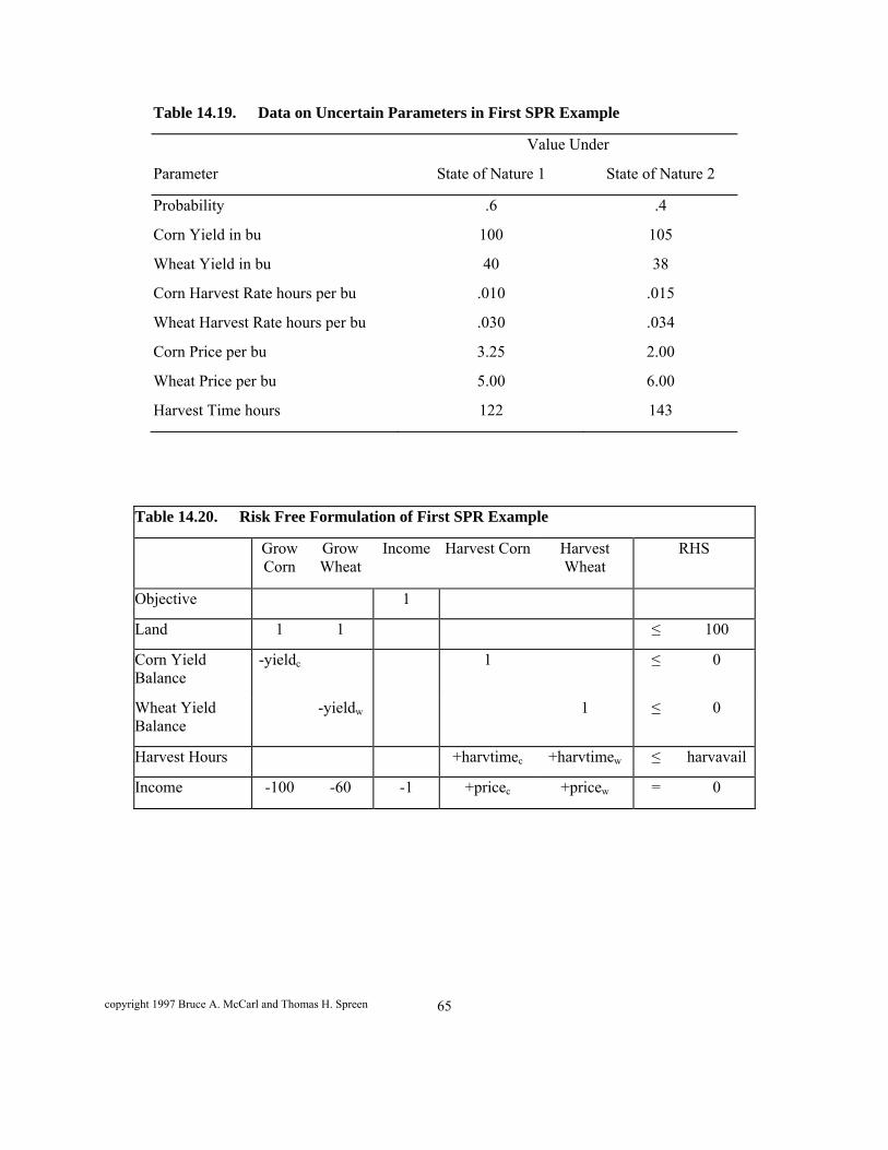
copyright 1997 Bruce A. McCarl and Thomas H. Spreen 65
Table 14.19. Data on Uncertain Parameters in First SPR Example
Value Under
Parameter State of Nature 1 State of Nature 2
Probability .6 .4
Corn Yield in bu 100 105
Wheat Yield in bu 40 38
Corn Harvest Rate hours per bu .010 .015
Wheat Harvest Rate hours per bu .030 .034
Corn Price per bu 3.25 2.00
Wheat Price per bu 5.00 6.00
Harvest Time hours 122 143
Table 14.20. Risk Free Formulation of First SPR Example
Grow Corn
Grow Wheat
Income Harvest Corn Harvest Wheat
RHS
Objective 1
Land 1 1 ≤ 100
Corn Yield Balance
-yieldc 1 ≤ 0
Wheat Yield Balance
-yieldw 1 ≤ 0
Harvest Hours +harvtimec +harvtimew ≤ harvavail
Income -100 -60 -1 +pricec +pricew = 0

copyright 1997 Bruce A. McCarl and Thomas H. Spreen 66
Table 14.21. Formulation of First SPR Example State 1 State 2
Grow Corn
Grow Wht.
Inc. s1 Harv Corn s1
Harv Wht s1
Inc. s2 Harv Corn s2
Harv Wht s2
RHS
Objective .6 .4 max
Land 1 1 ≤ 100
S t a t e 1
Corn s1 -100 1 ≤ 0
Wheat s1 -40 1 ≤ 0
Harvest Hours s1 .010 .030 ≤ 122
Income s1 -100 -60 -1 3.25 5.00 = 0
S t a t e 2
Corn s2 -105 1 ≤ 0
Wheat s2 -38 1 ≤ 0
Harvest Hours s2 .015 .034 ≤ 143
Income s2 -100 -60 -1 2.00 6.00 = 0

copyright 1997 Bruce A. McCarl and Thomas H. Spreen 67
Equation Slack Shadow Price
Objective 16476
Land 0 24.28
Corn s1 0 -1.95
Wheat s1 0 0.67
Harvest Hours s1 11.75 0
Income s1 0 -0.6
Corn s2 0 -3.00
Wheat s2 0 0.94
Harvest Hours s2 0 98.23
Income s2 0 -0.4
Variable
Solution Value
Marginal Cost
Grow Corn 48.8 0
Grow Wheat 51.2 0
Income S1 18144 0
Harvest Corn s1 4876 0
Harvest Wheat s1 2049 0
Income S2 13972 0
Harvest Corn s2 5120 0
Harvest Wheat s2 1947 0
copyright 1997 Bruce A. McCarl and Thomas H. Spreen 68
Table 14.23. Second SPR Example Formulation (Partial Tableau)
Corn Soy Wht Avg Cost
Pos ProtDev s1
Neg ProtDev s1
Pos Eng Dev s1
Neg Eng Dev s1
Cost s1
Pos CostDevs1
Negs CostDevs1
Pos Prot Dev s2
Neg ProtDev s2
Pos Eng Dev s2
Neg Eng Dev s2
Cost s2
Pos CostDevs2
NegCostDevs2
Objective 1 + + + + Total Feed 1 1 1 = 1
Average Cost 1 -.25 -.25 = 0
Protein-s1 0.23 1.12 0.51 -1 1 = 0.6
Energy -s1 1.15 0.26 1.05 -1 1 = 0.9
Cost-s1 0.03 0.06 0.04 0.50 1.50 1.00 0.10 -1 = 0
Cost dev s1 -1 1 -1 1 = 0
Protein-s2 0.17 1.08 0.59 -1 1 = 0.6
Energy -s2 1.10 0.31 0.95 -1 1 = 0.9
Cost-s2 .03 .06 .04 0.50 1.50 1.00 0.10 -1 = 0
Cost dev s2 -1 1 -1 1 = 0
copyright 1997 Bruce A. McCarl and Thomas H. Spreen 69
Table 14.24. Second SPR Example Risk Neutral Solution
Slack
Shadow Price
Slack
Shadow Price
Objective 0.067 Corn Purchase 0.283 0
Total Feed 0 -0.14 Soybean Purchase 0.362 0
Average Cost 0.00 1. Wheat Purchase 0.355 0
Protein-s1 0 0.125 Average Cost 0.067 0
Energy -s1 0 0.025 Pos Protein Dev s1 0.052 0
Cost-s1 0 252.66 Neg Protein Dev s1 0. 0.50
Cost dev s1 0 0.00 Pos Energyn Dev s1 0.00 0
Protein-s2 0 0.125 Neg Energy Dev s1 0.108 0
Energy -s2 0 0.025 Cost - s1 0.081 0
Cost-s2 0 0.25 Pos Cost Dev - s1 0.014 0
Cost dev s2 0 0 Neg Cost Dev - s1 0.00 0
Protein-s3 0 -.366 Pos Protein Dev s2 0.049 0
Energy -s3 0 0.025 Neg Protein Dev s2 0.000 0.50
Cost-s3 0 0.25 Pos Energyn Dev s2 0. 0.275
Cost dev s3 0 0 Neg Energyn Dev s2 0.140 0
Protein-s4 0 .08 Cost - s2 0.083 0
Energy -s4 0 .025 Pos Cost Dev - s2 .016 0
Cost-s4 0 0.25 Neg Cost Dev - s2 0.00 0
Cost dev s4 0 0.00 Pos Protein Dev s3 0. 0.491
Neg Protein Dev s3 0. 0.009
Pos Energy Dev s3 0.275
Neg Energy Dev s3 0.080 0
Cost - s3 0.052 0
Pos Cost Dev - s3 0.00 0
Neg Cost Dev - s3 0.014 0
Pos Protein Dev s4 0. 0.205
Neg Protein Dev s4 0. 0.295
Pos Energyn Dev s4 0. 0.275
Neg Energy Dev s4 0.067 0
Cost - s4 0.051 0
Pos Cost Dev - s4 0. 0
Neg Cost Dev - s4 0.016 0
copyright 1997 Bruce A. McCarl and Thomas H. Spreen 70
Aversion
RAP 0 0.1 0.2 0.3 0.4 0.500 0.600
Corn 0.283 0.249 0.245 0.244 0.288 0.296 0.297
Soybeans 0.362 0.330 0.327 0.326 0.340 0.342 0.342
Wheat 0.355 0.422 0.428 0.430 0.372 0.363 0.361
Avgcost 0.067 0.067 0.067 0.067 0.071 0.071 0.071
Cost s1 0.081 0.074 0.073 0.073 0.071 0.071 0.071
Cost s2 0.083 0.080 0.080 0.080 0.074 0.073 0.073
Cost s3 0.052 0.066 0.067 0.068 0.071 0.071 0.071
Cost s4 0.051 0.048 0.048 0.048 0.067 0.070 0.071
Std Error 0.015 0.012 0.012 0.012 0.002 0.001 0.001
RAP is the risk aversion parameter.

copyright 1997 Bruce A. McCarl and Thomas H. Spreen 71
Table 14.26. Example Tableau for Third SPR Problem Average
Ending Net Worth
Period 1 Period 2 Stage 3
Period 2 State 1 Period 2 State 2 State 1 State 2 Period 3 State A Period 3 State B Period 3 State A Period 3 State B Sell Keep Sell Keep Sell Keep Sell End Worth Sell End
WorthSell End
WorthSell End
Worth Objective 1 max
Starting Stock 1 1 ≤ 100
Avg End Worth 1 -0.42 -0.28 -0.21 -0.09 = 0
Stock Kept pd 1 to 2 s1 -1 1 1 ≤ 0
Stock Kept pd 1 to 2 s2 -1 1 1 ≤ 0 P2 S1
Stock Kept pd 2 to 3 s1-sA -1 1 ≤ 0
Ending Worth s1-sA 2.1412 2.332 2.18 -1 = 0
Stock Kept pd 2 to 3 s1-sB -1 1 ≤ 0
Ending Worth s1-sB 2.1008 2.288 2.44 -1 = 0
P2 S2
Stock Kept pd 2 to 3 s2-sA -1 1 ≤ 0
Ending Worth s2-sA 2.1828 2.193 2.18 -1 = 0
Stock Kept pd 2 to 3 s2-sB -1 1 ≤ 0
Ending Worth s2-sB 2.1012 2.111 2.44 -1 = 0
copyright 1997 Bruce A. McCarl and Thomas H. Spreen 72
Table 14.27. Solution for Third SPR Example Variable Value Reduced Cost Variable Slack Shadow Price
Average Ending Net Worth 229.748 0 Objective 229.748 Sell In Period 1 0 -0.162 Starting Stock 0 2.297
Keep From Period 1 to 2 100 0 Avg End Worth 0 1
Sell In Period 2 Under State 1 100 0 Stock Kept pd 1 to 2 s1 0 1.62
Keep From Period 2 to 3 Under State 1 0 -0.021 Stock Kept pd 1 to 2 s1 0 0.677
Sell In Period 2 Under State 2 0 -0.027 Stock Kept pd 2 to 3 s1-s1 0 0.916
Keep From Period 2 to 3 Under State 2 100 0 Ending Worth s1-s1 0 -0.42
Sell in Period 3 Under State 1 -- State A 0 0 Stock Kept pd 2 to 3 s1-s2 0 0.683
Ending Worth Under State 1 -- State A 233.2 0 Ending Worth s1-s2 0 -0.28
Sell In Period 3 Under State 1 -- State B 0 0 Stock Kept pd 2 to 3 s2-s1 0 0.458
Ending Worth Under State 1 -- State B 228.8 0 Ending Worth s2-s1 0 -0.21
Sell In Period 3 Under State 2 -- State A 100 0 Stock Kept pd 2 to 3 s2-s2 0 0.22
Ending Worth Under State 2 -- State A 218 0 Ending Worth s2-s2 0 -0.09
Sell In Period 3 Under State 2 -- State B 100 0 Ending Worth Under State 2 -- State B 244 0

copyright 1997 Bruce A. McCarl and Thomas H. Spreen 73
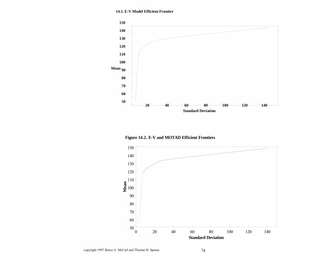
copyright 1997 Bruce A. McCarl and Thomas H. Spreen 74
14.1. E-V Model Efficient Frontier
20 40 60 80 100 120 14050
60
70
80
90
100
110
120
130
140
150
Standard Deviation
Mean
Figure 14.2. E-V and MOTAD Efficient Frontiers
0 20 40 60 80 100 120 14050
60
70
80
90
100
110
120
130
140
150
Standard Deviation
Mea
n

copyright 1997 Bruce A. McCarl and Thomas H. Spreen 75
Pre-Planting Decisions
Planting Decisions
Harvesting Decisions
B1C1 B2C1 B2C2B1C1
B2 B1