chapter1
TRANSCRIPT
COURSE:COURSE:DIGITAL SIGNAL TRANSFORMS & DIGITAL SIGNAL TRANSFORMS &
APPLICATIONSAPPLICATIONS
Instructor: Hoang Le Uyen Thuc
Electronic and Telecommunication Engineering Department
Danang University of Technology
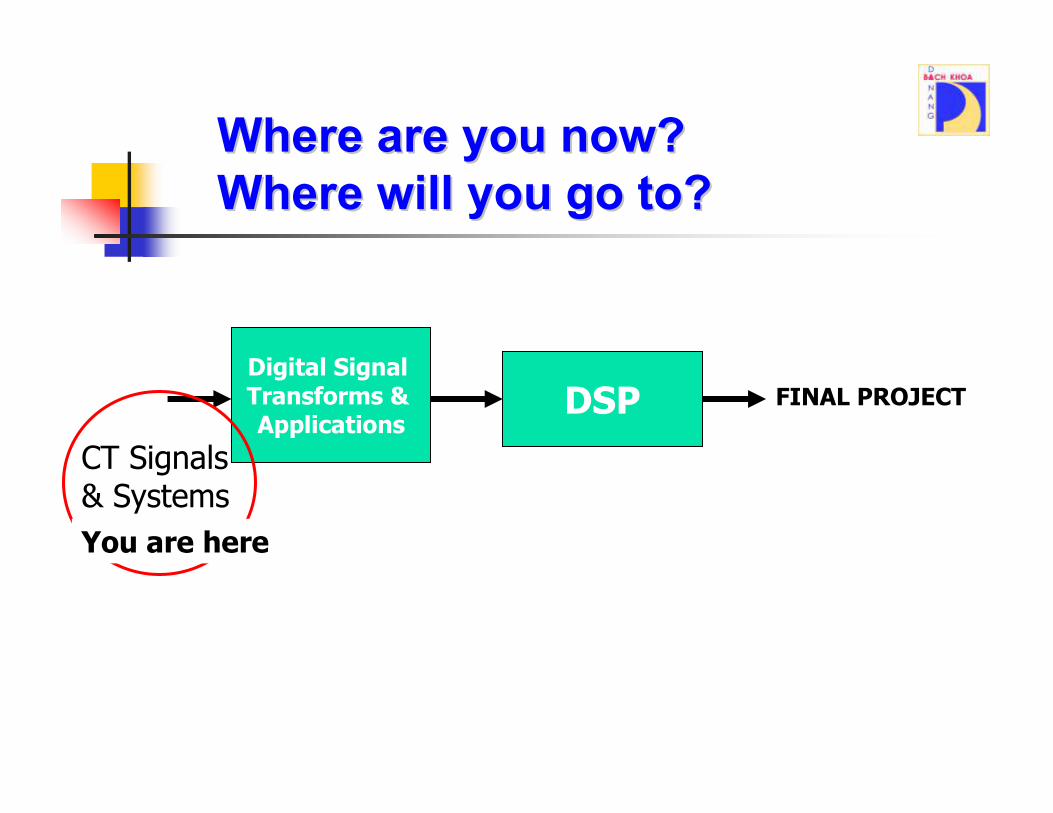
Where are you now? Where are you now? Where will you go to?Where will you go to?
Digital Signal Transforms & Applications
DSP FINAL PROJECT
CT Signals & Systems
You are here
GoalsGoals
1. To provide students the basic digital signal
transforms such as Z-transform, Discrete-Time
Fourier Transform and Discrete Fourier Transform
and their applications in analysis and synthesis of
DSP systems
2. To equip students the basic 2D transforms using in
image processing

GradingGrading
1. Homework: 30%
Submit right before the examination
2. Exam: 70%
Things can be brought into the exam. room: pen/pencils,
ruler, eraser, clock, calculator, white drafts, two A4
papers
Each paper is two-side personal writing
Exam. duration: 60 minutes
Textbooks and ReferencesTextbooks and References
Textbook: John G.Proakis & Dimitris G. Manolakis - Digital signal
processing - Prentice Hall, New Jersey 2006
References:
[1] Nguyễn Quốc Trung - Xử lý tín hiệu & lọc số Tập 1- NXB Khoa
học & kỹ thuật, Hà Nội 2001
[2] Joyce Van de Vegte - Fundamentals of Digital Signal
Processing - Prentice Hall 2002
[3] Vinay K.Ingle & John G.Proakis - Digital Signal Processing
using Matlab - Book Ware Companion Series 2007
Schedule:Schedule:
Chapter 1: Digital Signals and Systems (5 hrs)
Chapter 2: Z-transforms and applications (5 hrs)
Chapter 3: Discrete-time Fourier Transform and applications (5
hrs)
Chapter 4: Discrete Fourier Transform and applications (5 hrs)
Chapter 5: 2D Transforms and application in image processing (5
hrs)
Review and class discussion (5 hrs)

CHAPTER 1:CHAPTER 1:
DIGITAL SIGNALS & SYSTEMSDIGITAL SIGNALS & SYSTEMS
Lesson #1: A big picture about Digital Signal Processing
Lesson #2: Digital signals
Lesson #3: Digital systems
Duration: 5 hrs

Lecture #1:Lecture #1: A big picture about A big picture about
Digital Signal Processing Digital Signal Processing
Duration: 1 hr
Outline:
1. Signals
2. Digital Signal Processing (DSP)
3. Why DSP?
4. DSP applications
SignalsSignals
Function of independent variables such as time, distance,
position, temperature
Convey information
Examples:
1D signal: speech, music, biosensor…
2D signal: image
2.5D signal: video (2D image + time)
3D signal: animated

11--D signalsD signals
Color imageSpeech signal
ECG
EEG
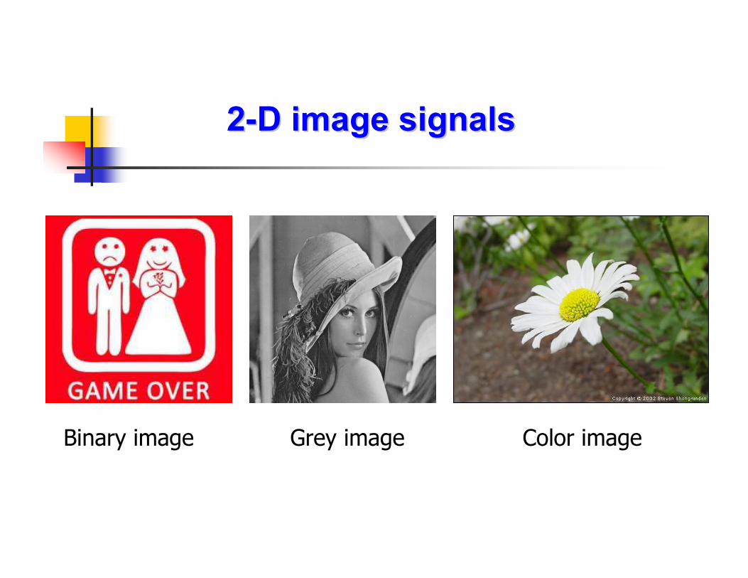
22--D image signalsD image signals
Binary image Color imageGrey image
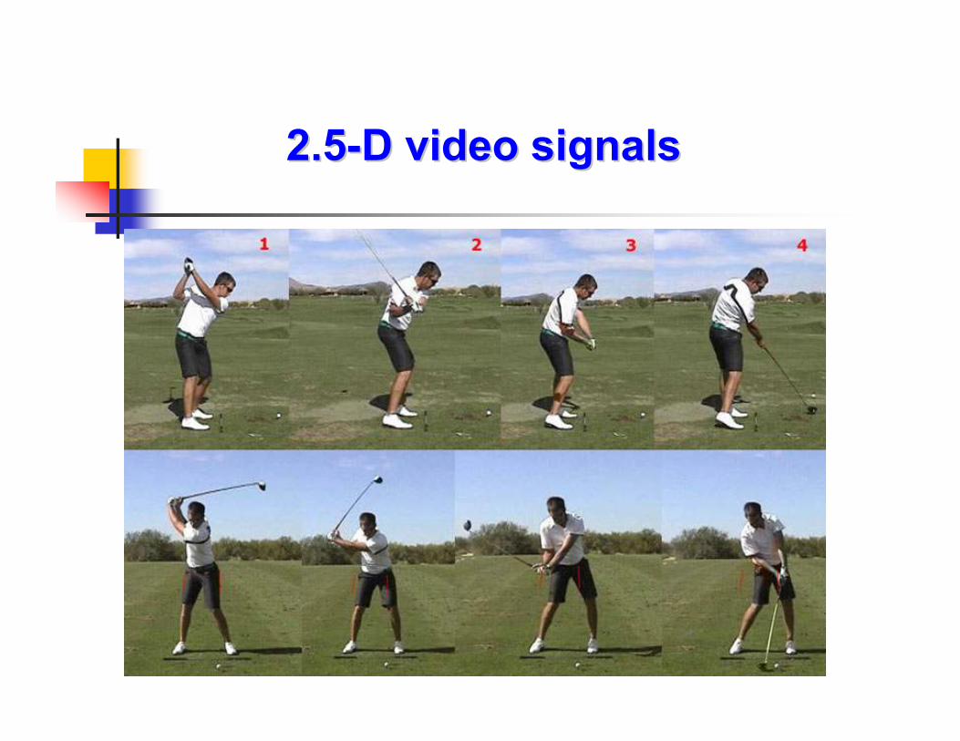
2.52.5--D video signalsD video signals
33--D animated signalsD animated signals
What is Digital Signal Processing?What is Digital Signal Processing?
Represent a signal by a sequence of numbers (called a
"discrete-time signal” or "digital signal").
Modify this sequence of numbers by a computing process
to change or extract information from the original signal
The "computing process" is a system that converts one
digital signal into another— it is a "discrete-time system” or
"digital system“.
Transforms are tools using in computing process
DiscreteDiscrete--time signal vs. time signal vs. continuouscontinuous--time signaltime signal
Continuous-time signal:
- define for a continuous duration of time
- sound, voice…
Discrete-time signal:
- define only for discrete points in time (hourly, every second, …)
- an image in computer, a MP3 music file
- amplitude could be discrete or continuous
- if the amplitude is also discrete, the signal is digital.
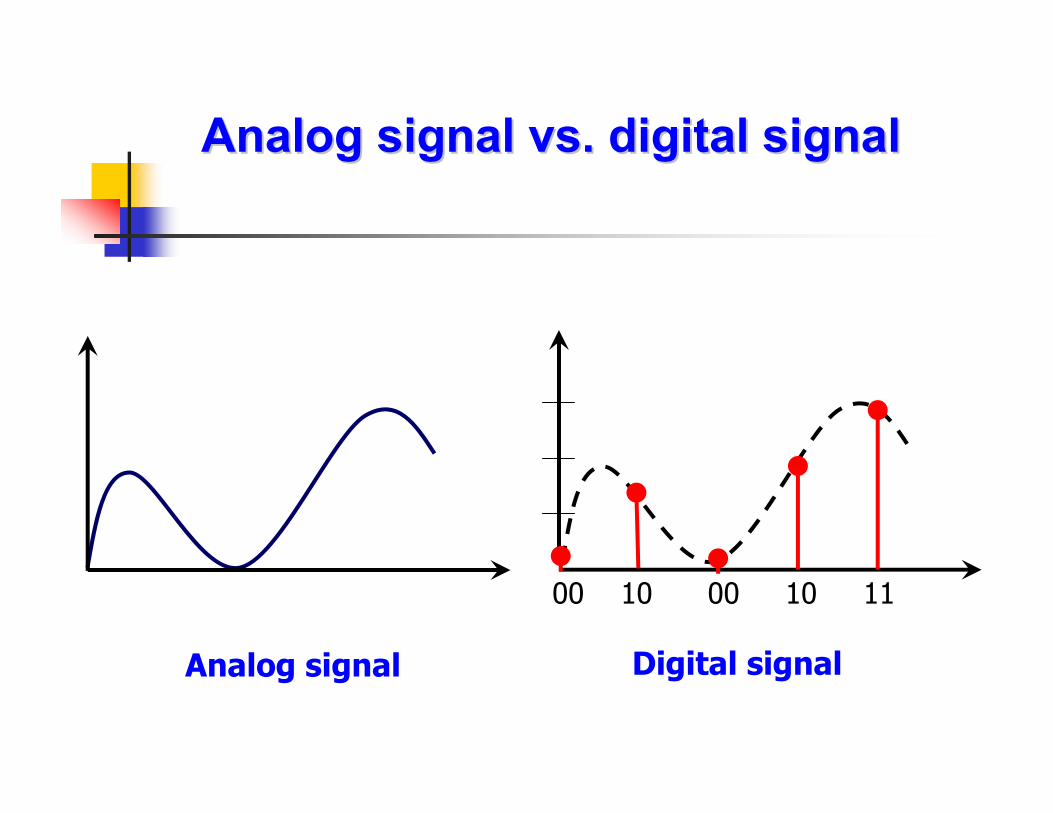
Analog signal vs. digital signalAnalog signal vs. digital signal
Analog signal Digital signal
00 10 00 10 11
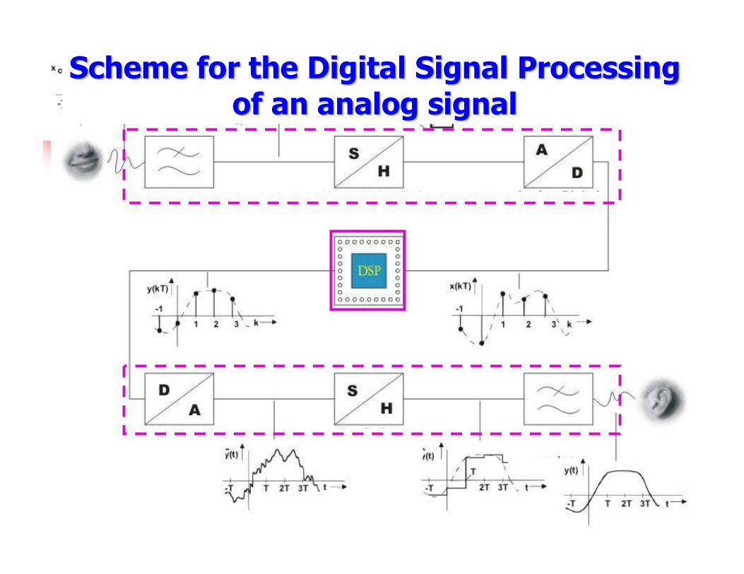
Scheme for the Digital Signal Processing Scheme for the Digital Signal Processing of an analog signalof an analog signal
Digital Signal Processing Digital Signal Processing ImplementationImplementation
Performed by:
Special-purpose (custom) chips: application-specific integrated
circuits (ASIC)
Field-programmable gate arrays (FPGA)
General-purpose microprocessors or microcontrollers (µP/µC)
General-purpose digital signal processors (DSP processors)
DSP processors with application-specific hardware (HW)
accelerators

Digital Signal Processing Digital Signal Processing implementationimplementation
Digital Signal Processing Digital Signal Processing ImplementationImplementation
Use basic operations of addition,
multiplication and delay
Combine these operations to accomplish
processing: a discrete-time input signal
another discrete-time output signal
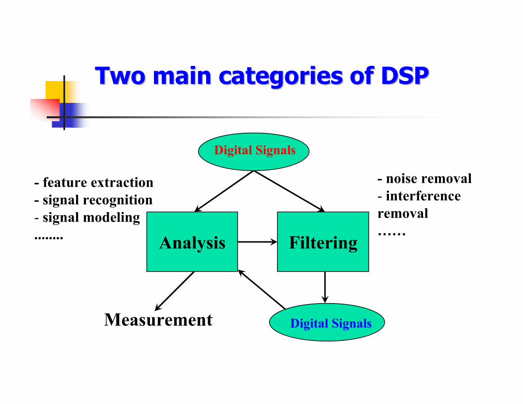
Two main categories of DSPTwo main categories of DSP
Analysis Filtering
Measurement Digital Signals
- feature extraction
- signal recognition
- signal modeling
........
- noise removal
- interference
removal
……
Digital Signals
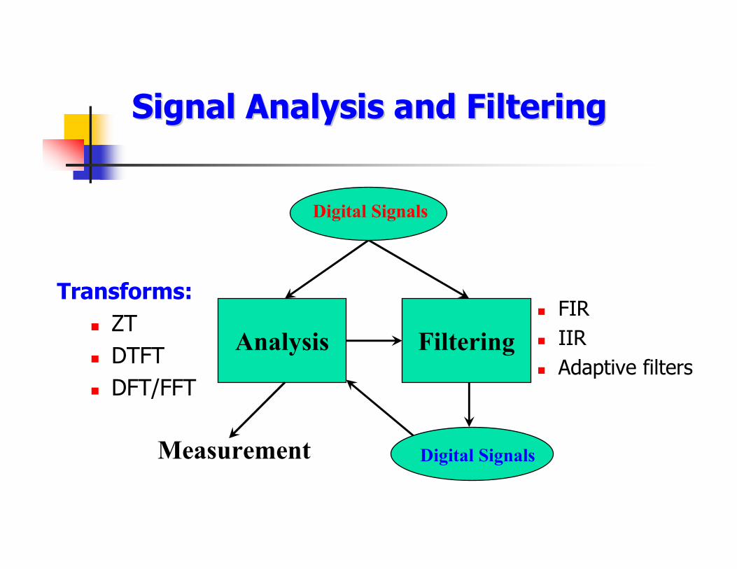
Signal Analysis and FilteringSignal Analysis and Filtering
Analysis Filtering
Measurement Digital Signals
Digital Signals
Transforms:
ZT
DTFT
DFT/FFT
FIR
IIR
Adaptive filters
Advantages of Digital Advantages of Digital Signal ProcessingSignal Processing
Flexible: re-programming ability
More reliable
Smaller, lighter less power
Easy to use, to develop and test (by using the
assistant tools)
Suitable to sophisticated applications
Suitable to remote-control applications
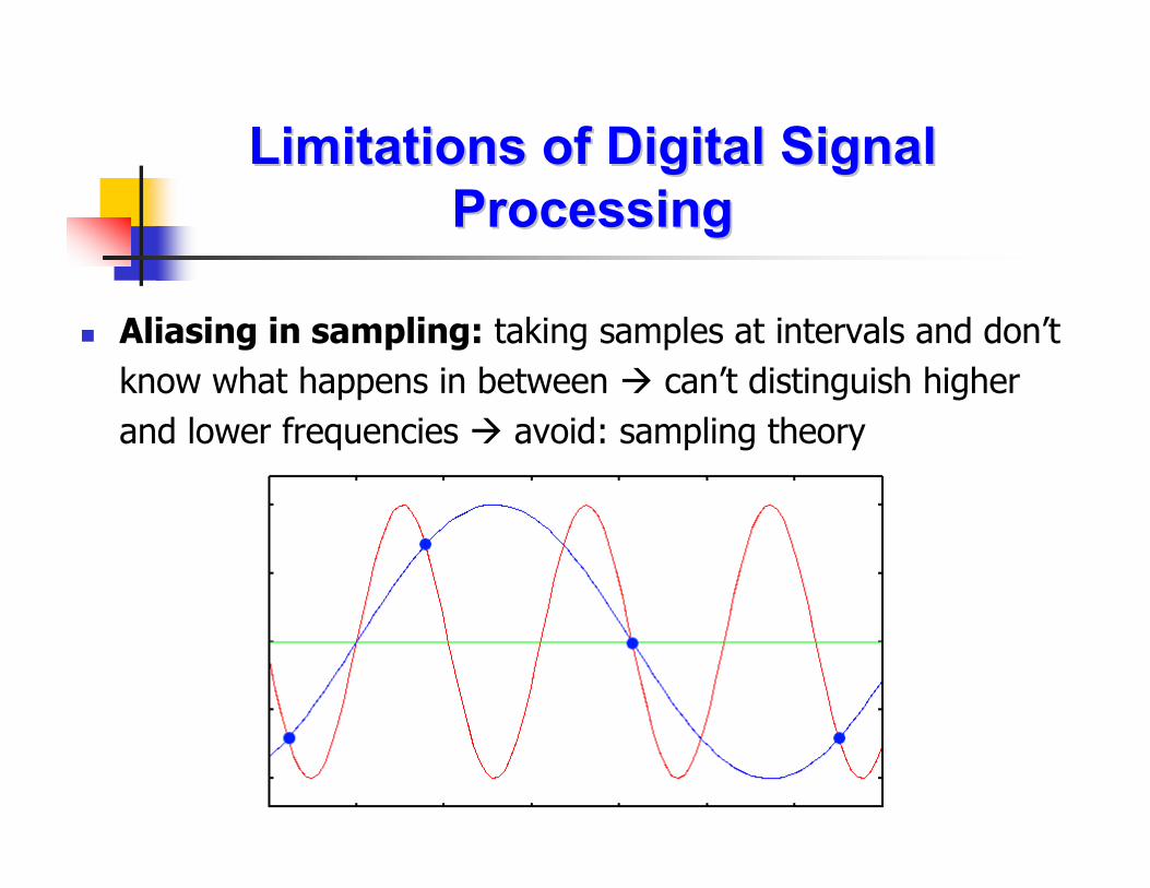
Limitations of Digital Signal Limitations of Digital Signal ProcessingProcessing
Aliasing in sampling: taking samples at intervals and don’t
know what happens in between can’t distinguish higher
and lower frequencies avoid: sampling theory
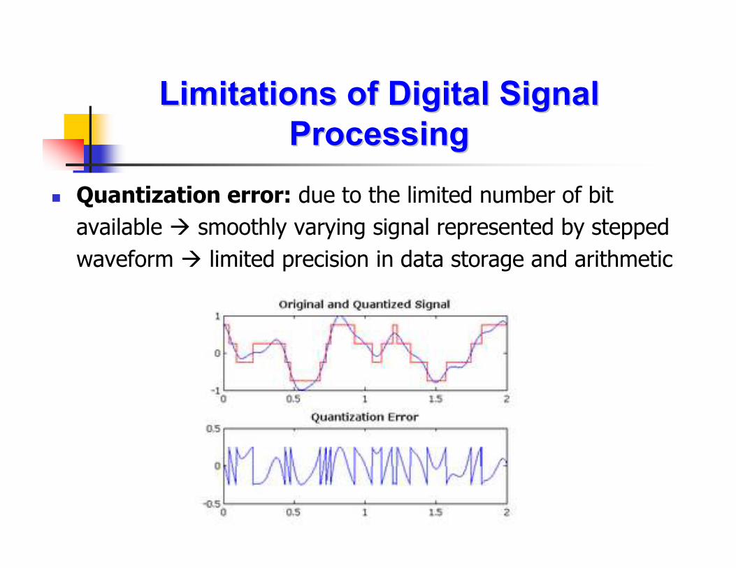
Limitations of Digital Signal Limitations of Digital Signal ProcessingProcessing
Quantization error: due to the limited number of bit
available smoothly varying signal represented by stepped
waveform limited precision in data storage and arithmetic
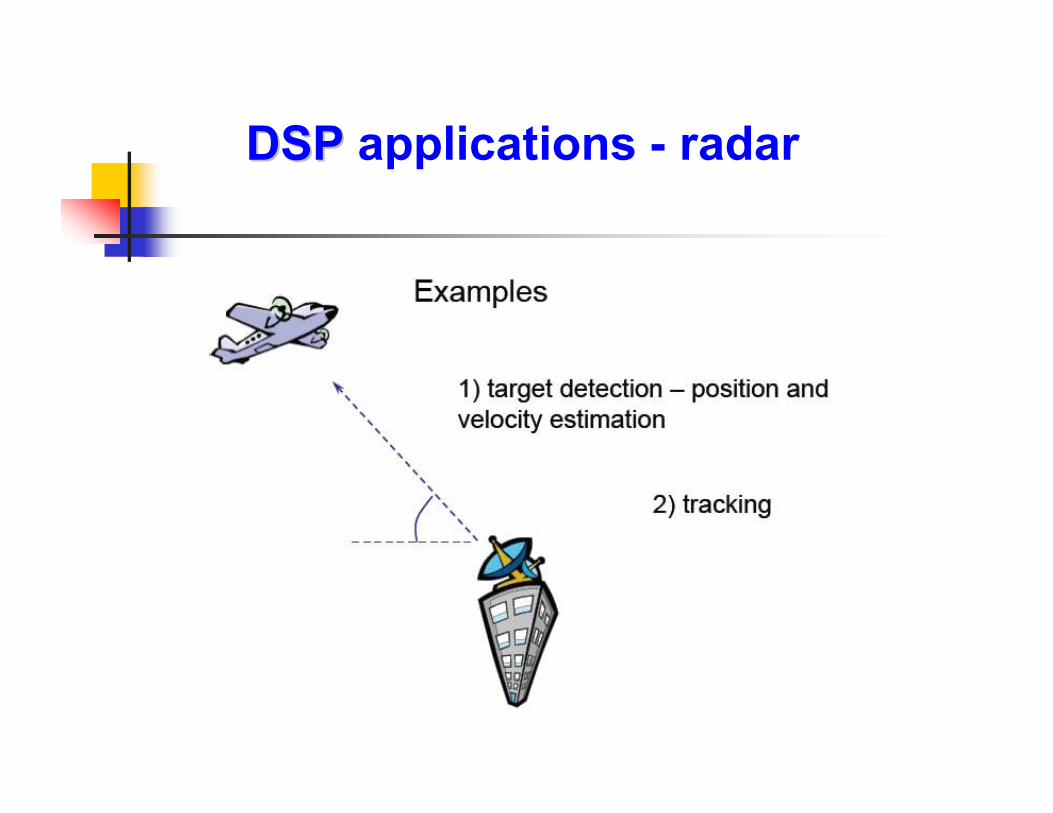
DSP DSP applications - radar
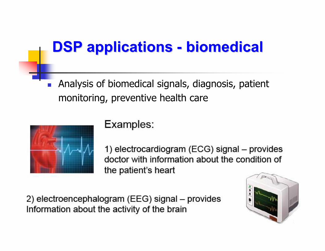
DSP applications DSP applications -- biomedicalbiomedical
Analysis of biomedical signals, diagnosis, patient
monitoring, preventive health care
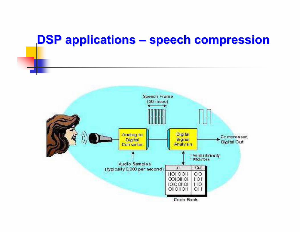
DSP applications DSP applications –– speech compressionspeech compression
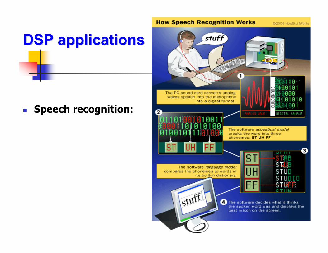
DSP applicationsDSP applications
Speech recognition:

DSP applications DSP applications -- communicationcommunication
Digital telephony: transmission of information in
digital form via telephone lines, modern technology,
mobile phone
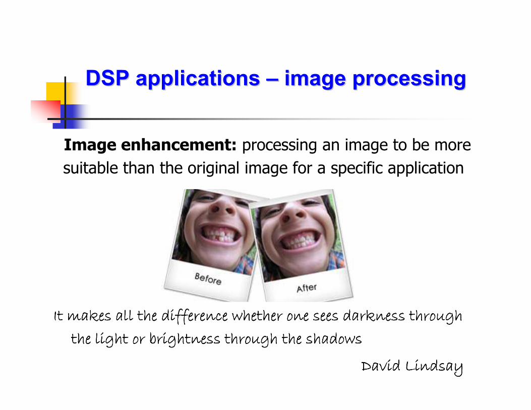
DSP applications DSP applications –– image processingimage processing
Image enhancement: processing an image to be more
suitable than the original image for a specific application
It makes all the difference whether one sees darkness through It makes all the difference whether one sees darkness through It makes all the difference whether one sees darkness through It makes all the difference whether one sees darkness through
the light or brightness through the shadowsthe light or brightness through the shadowsthe light or brightness through the shadowsthe light or brightness through the shadows
David LindsayDavid LindsayDavid LindsayDavid Lindsay
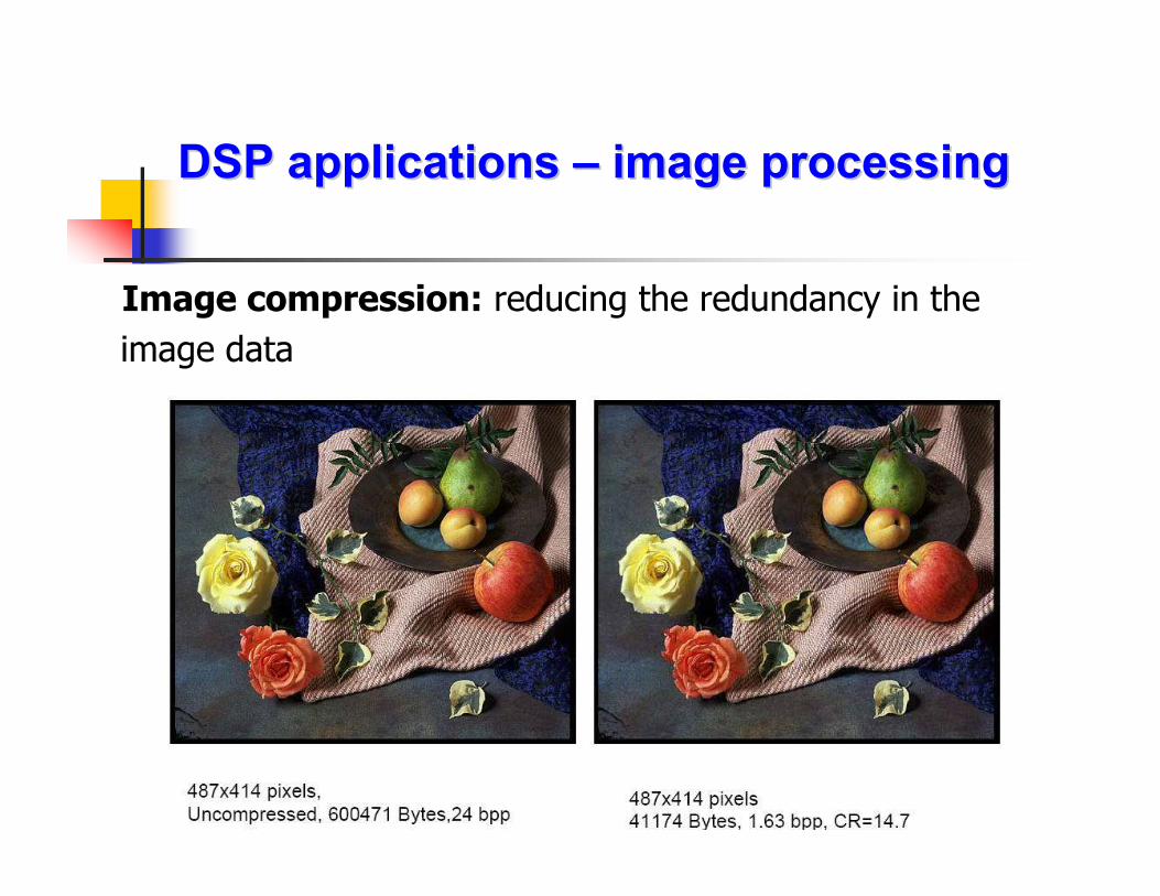
DSP applications DSP applications –– image processingimage processing
Image compression: reducing the redundancy in the
image data
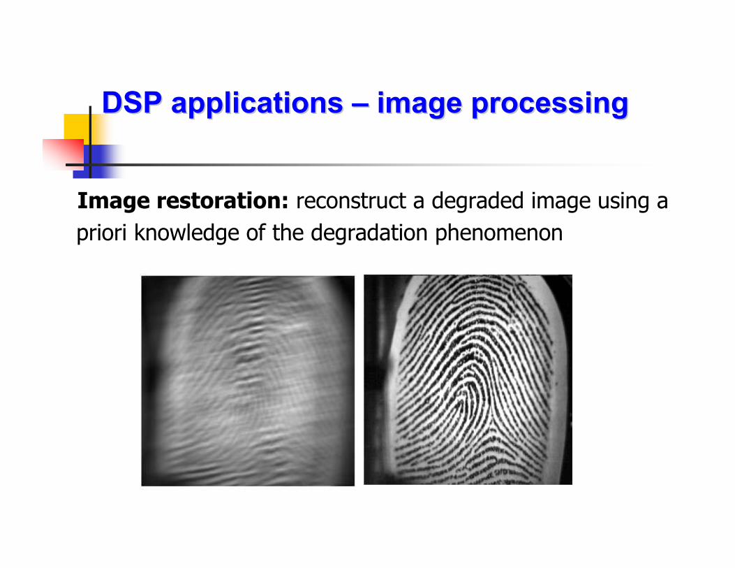
DSP applications DSP applications –– image processingimage processing
Image restoration: reconstruct a degraded image using a
priori knowledge of the degradation phenomenon

DSP applicationsDSP applications-- musicmusic
Recording, encoding, storing
Playback
Manipulation/mixing
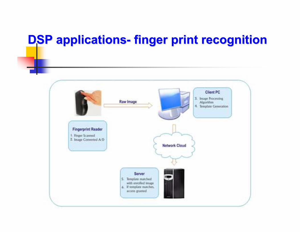
DSP applicationsDSP applications-- finger print recognitionfinger print recognition
Lecture #2Lecture #2
Digital (DT) SignalsDigital (DT) Signals
Duration: 2 hrs
Outline:
1. Representations of DT signals
2. Some elementary DT signals
3. Classification of DT signals
4. Simple manipulations of DT signals
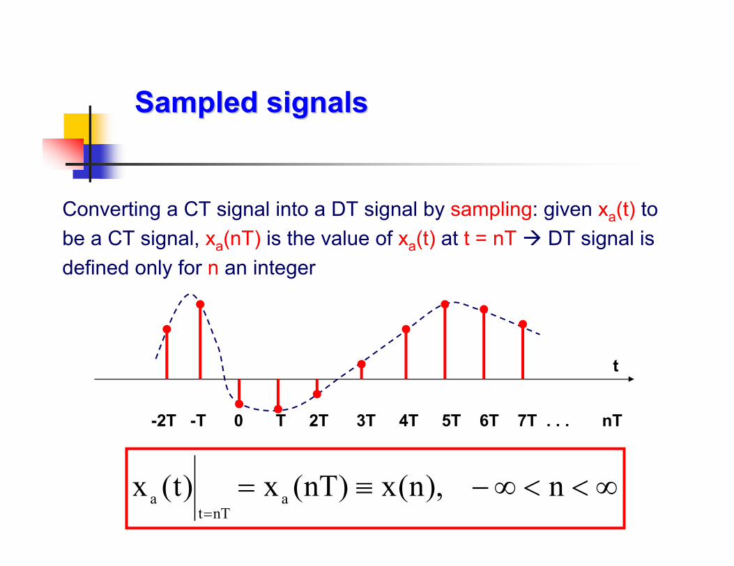
Converting a CT signal into a DT signal by sampling: given xa(t) to
be a CT signal, xa(nT) is the value of xa(t) at t = nT DT signal is
defined only for n an integer
∞<<∞−≡==
n),n(x)nT(x)t(xa
nTta
-2T -T 0 T 2T 3T 4T 5T 6T 7T . . . nT
t
Sampled signalsSampled signals

n 9 -1 0 1 2 3 4 9
x[n] 9 0 0 1 4 1 0 9
1. Functional representation
≠
=
=
=
n,0
2n,4
3,1n,1
]n[x
Representations of DT signalsRepresentations of DT signals
2. Tabular representation
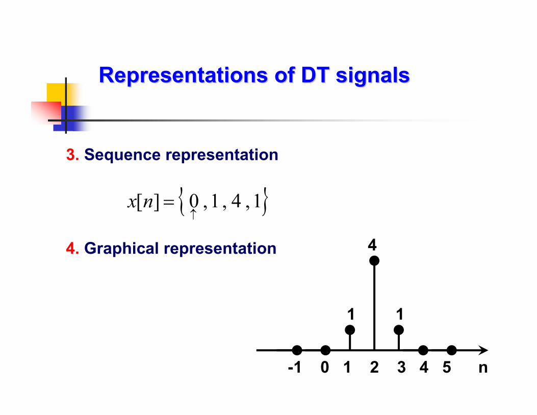
3. Sequence representation
Representations of DT signalsRepresentations of DT signals
4. Graphical representation
1,4,1,0][↑
=nx
-1 0 1 2 3 4 5 n
4
1 1
1. Unit step sequence
2. Unit impulse signal
3. Sinusoidal signal
4. Exponential signal
Some elementary DT signalsSome elementary DT signals
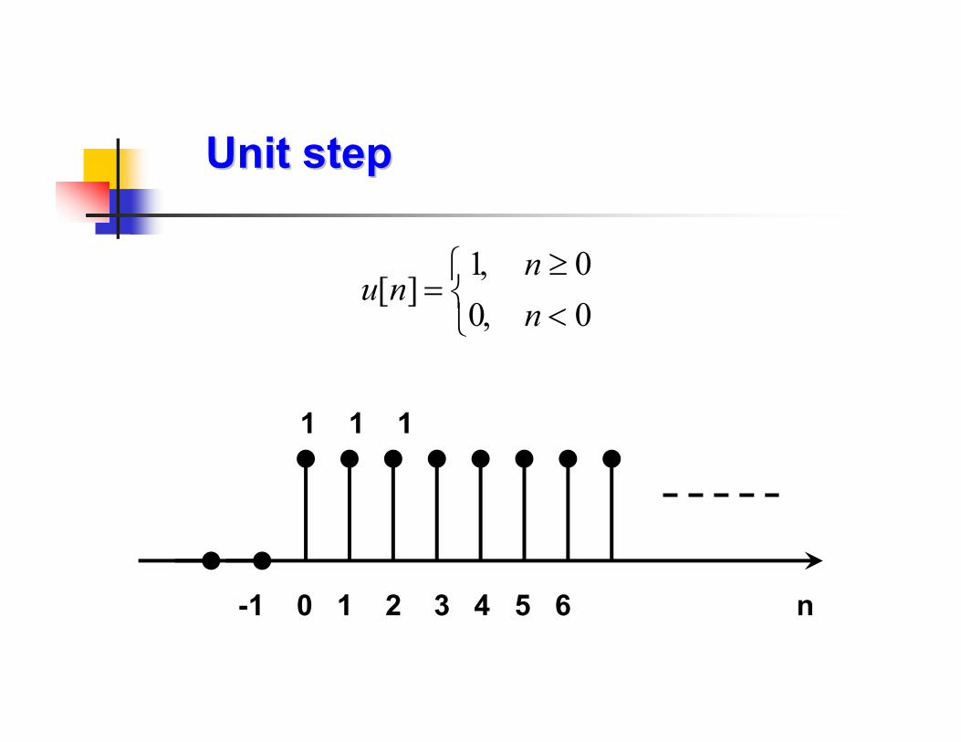
1 0[ ]
0 0
nu n
n
, ≥=
, <
-1 0 1 2 3 4 5 6 n
1 1 1
Unit stepUnit step
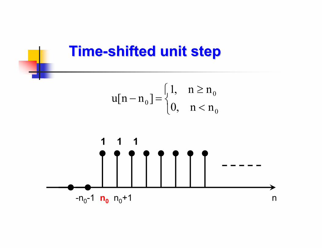
-n0-1 n0 n0+1 n
1 1 1
TimeTime--shifted unit stepshifted unit step
<
≥=−
0
0
0nn,0
nn,1]nn[u

Unit impulseUnit impulse
1 0[ ]
0 0
nn
nδ
, ==
, ≠
-2 -1 0 1 2 3 n
1
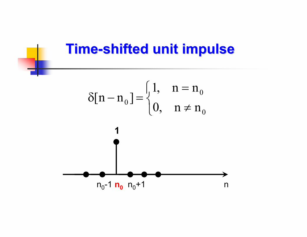
TimeTime--shifted unit impulseshifted unit impulse
n0-1 n0 n0+1 n
1
≠
==−δ
0
0
0nn,0
nn,1]nn[
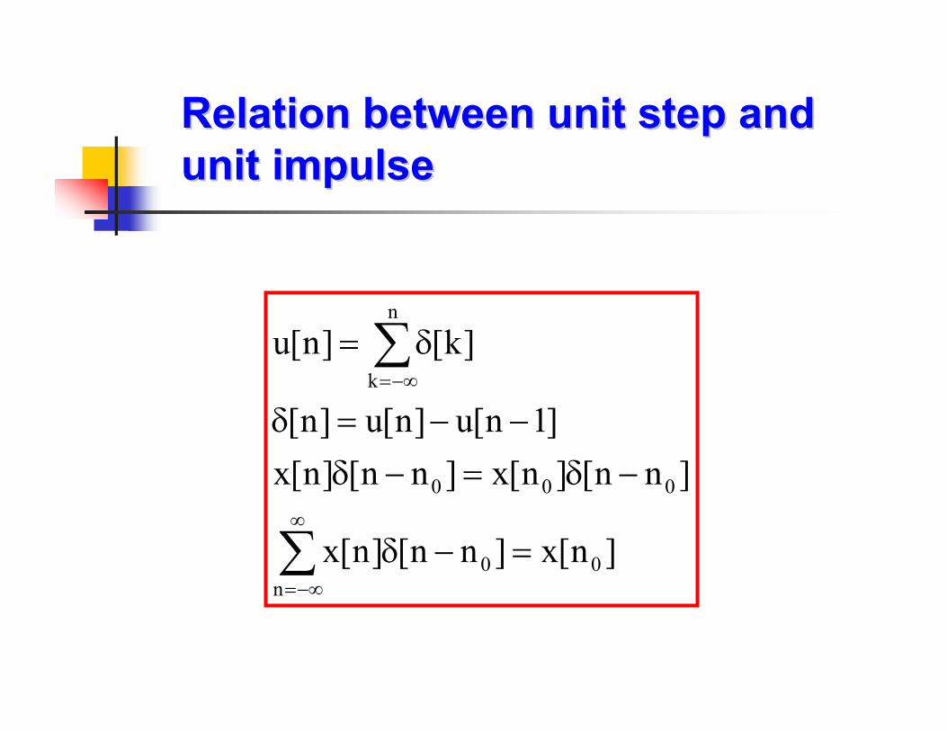
Relation between unit step and Relation between unit step and unit impulseunit impulse
]n[x]nn[]n[x
]nn[]n[x]nn[]n[x
]1n[u]n[u]n[
]k[]n[u
0
n
0
000
n
k
=−δ
−δ=−δ
−−=δ
δ=
∑
∑
∞
−∞=
−∞=

Sinusoidal signalSinusoidal signal
+∞<<∞−θ+π=
+∞<<∞−θ+Ω=
n),nF2cos(A
n),ncos(A)n(x
-20 -15 -1 0 -5 0 5 1 0 15 20-1 .5
-1
-0 .5
0
0 .5
1
1 .5

Exponential signalExponential signal
nCa]n[x =
1. If C and a are real, then x[n] is a real exponential
a > 1 growing exponential
0 < a < 1 shrinking exponential
-1 < a < 0 alternate and decay
a < -1 alternate and grows
2. If C or a is complex, then x[n] is a complex exponential
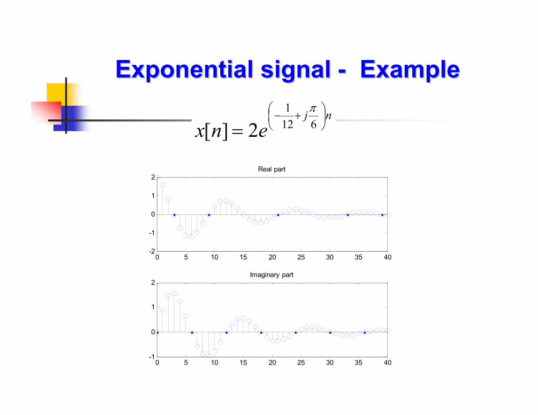
Exponential signal Exponential signal -- ExampleExample
nj
enx
+−
= 612
1
2][
π
0 5 10 15 20 25 30 35 40-2
-1
0
1
2Real part
0 5 10 15 20 25 30 35 40-1
0
1
2Imaginary part
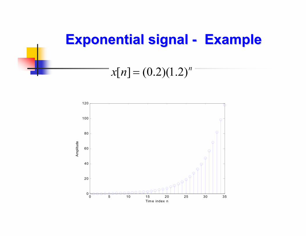
Exponential signal Exponential signal -- ExampleExample
nnx )2.1)(2.0(][ =
0 5 10 15 20 25 30 350
20
40
60
80
100
120
Tim e index n
Am
plit
ude
Periodic and aperiodic signals
Symmetric (even) and antisymmetric (odd) signals
Energy and power signals
Classification of DT signalsClassification of DT signals

Periodic signals: important, both for practical
reasons and for mathematical analysis
DT sinusoidal signal is periodic only if its frequency f
is rational number
Periodic and Aperiodic signalsPeriodic and Aperiodic signals

ExamplesExamples
6
1[ ]j n
x n eπ
=
32 5[ ] sin( 1)x n nπ= +
3[ ] cos(2 )x n n π= −
Determine which of the signals below are periodic. For the ones that are, find the fundamental period and fundamental frequency
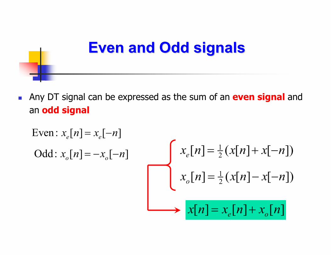
Any DT signal can be expressed as the sum of an even signal and
an odd signal
Even and Odd signalsEven and Odd signals
Even [ ] [ ]e ex n x n: = −
Odd [ ] [ ]o ox n x n: = − −12
[ ] ( [ ] [ ])ex n x n x n= + −
12
[ ] ( [ ] [ ])ox n x n x n= − −
[ ] [ ] [ ]e ox n x n x n= +
Given x[n] = [ 1 1 2 2 0 1 2 2 ]
Find xe[n] and xo[n]
ExamplesExamples
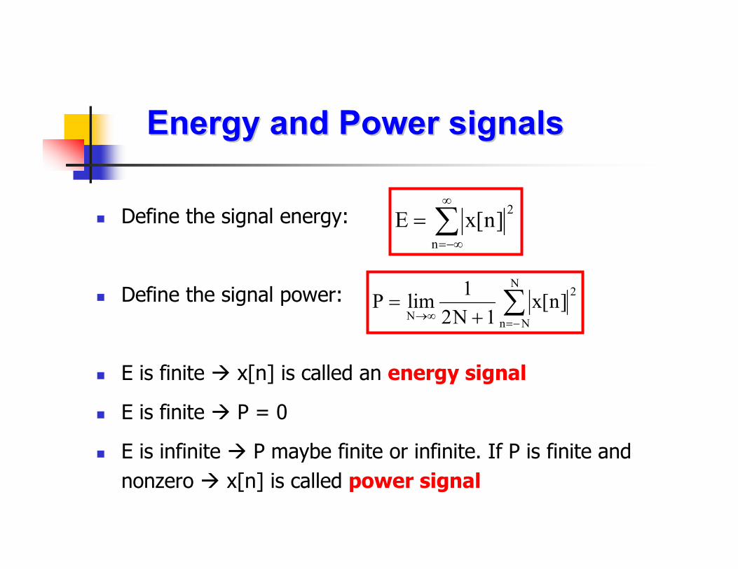
Define the signal energy:
Define the signal power:
E is finite x[n] is called an energy signal
E is finite P = 0
E is infinite P maybe finite or infinite. If P is finite and
nonzero x[n] is called power signal
Energy and Power signalsEnergy and Power signals
∑∞
−∞=
=n
2]n[xE
∑−=
∞→ +=
N
Nn
2
N]n[x
1N2
1limP
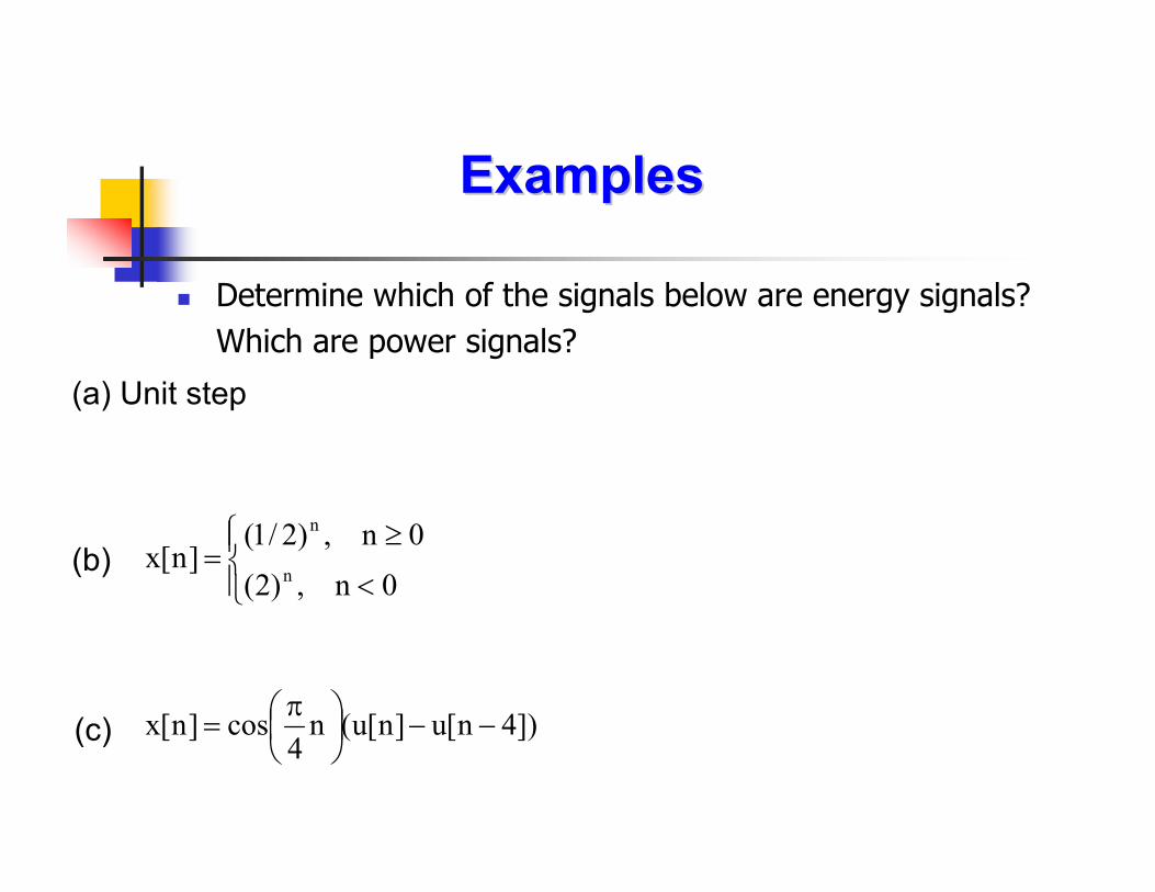
Determine which of the signals below are energy signals?
Which are power signals?
ExamplesExamples
(a) Unit step
(b)
<
≥=
0n,)2(
0n,)2/1(]n[x
n
n
(c) ])4n[u]n[u(n4
cos]n[x −−
π=
Transformation of time:
- Time shifting
- Time scaling
- Time reversal
Adding and subtracting signals
Simple manipulations of DT Simple manipulations of DT signalssignals

x[n] x[n - k]; k is an integer
k > 0: right-shift x[n] by |k| samples
(delay of signal)
k < 0: left-shift x[n] by |k| samples
(advance of signal)
Time shifting a DT signalTime shifting a DT signal
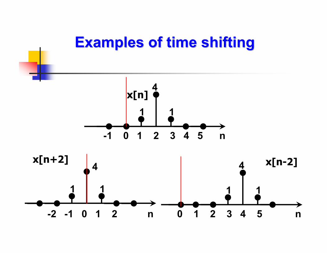
Examples of time shiftingExamples of time shifting
-1 0 1 2 3 4 5 n
4
1 1
x[n]
-2 -1 0 1 2 n
4
1 1
0 1 2 3 4 5 n
4
1 1
x[n-2]x[n+2]
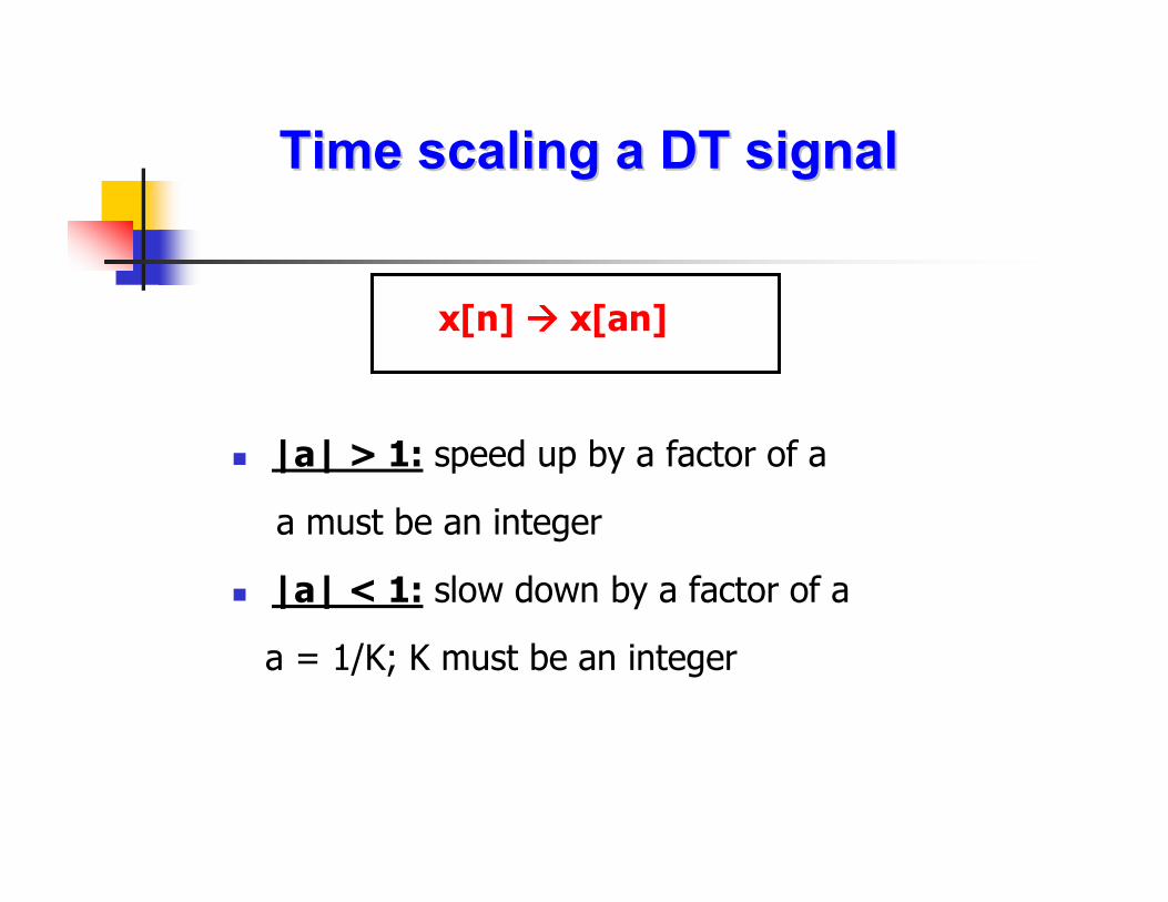
x[n] x[an]
|a| > 1: speed up by a factor of a
a must be an integer
|a| < 1: slow down by a factor of a
a = 1/K; K must be an integer
Time scaling a DT signalTime scaling a DT signal
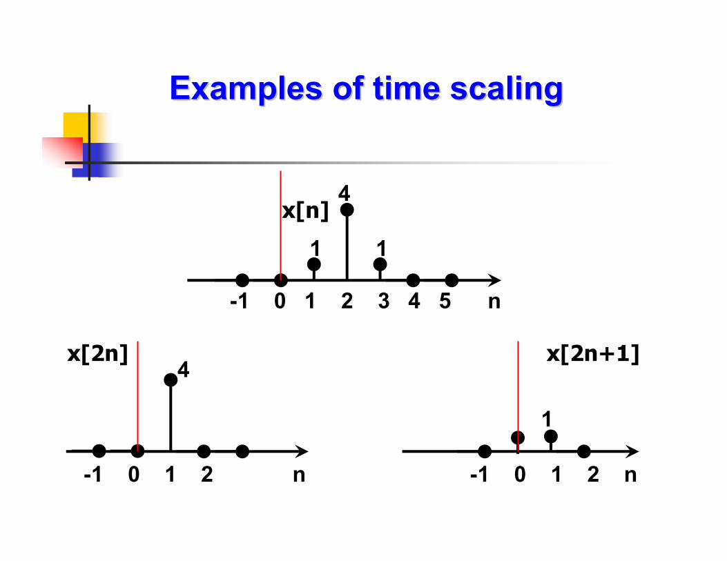
Examples of time scalingExamples of time scaling
-1 0 1 2 3 4 5 n
4
1 1
x[n]
-1 0 1 2 n
4
-1 0 1 2 n
1
x[2n+1]x[2n]

Examples of time scalingExamples of time scaling
-1 0 1 2 3 4 5 n
4
1 1
x[n]
??13
142
??11
000
y[n]=x[n/2]x[n]n
How do we find y[1] and y[3]??
One solution is linear interpolation used in a simple compression scheme
1/2
1/2
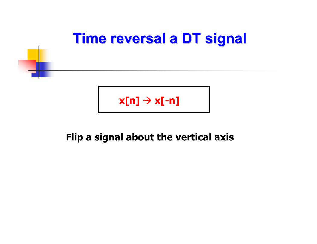
x[n] x[-n]
Flip a signal about the vertical axis
Time reversal a DT signalTime reversal a DT signal
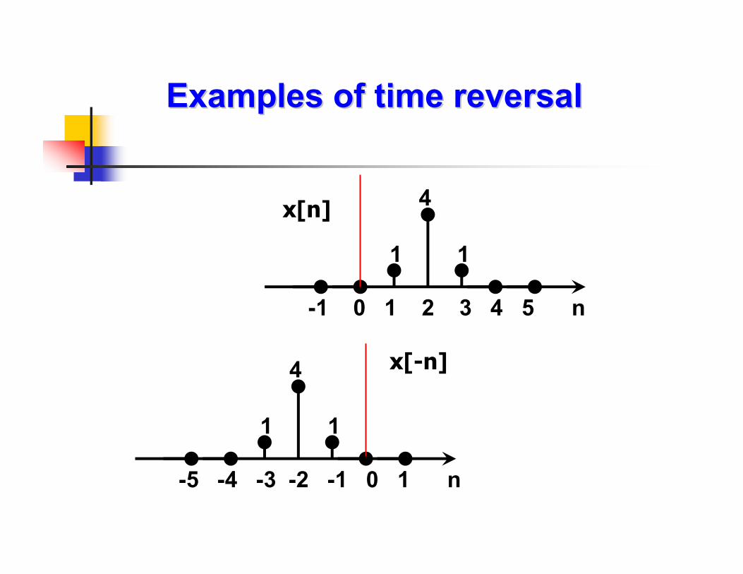
Examples of time reversalExamples of time reversal
-1 0 1 2 3 4 5 n
4
1 1
x[n]
-5 -4 -3 -2 -1 0 1 n
4
1 1
x[-n]
x[n] x[-n-k]
Method 1: Flip first, then shift
Method 2: Shift first, then flip
Combining time reversal and Combining time reversal and time shiftingtime shifting
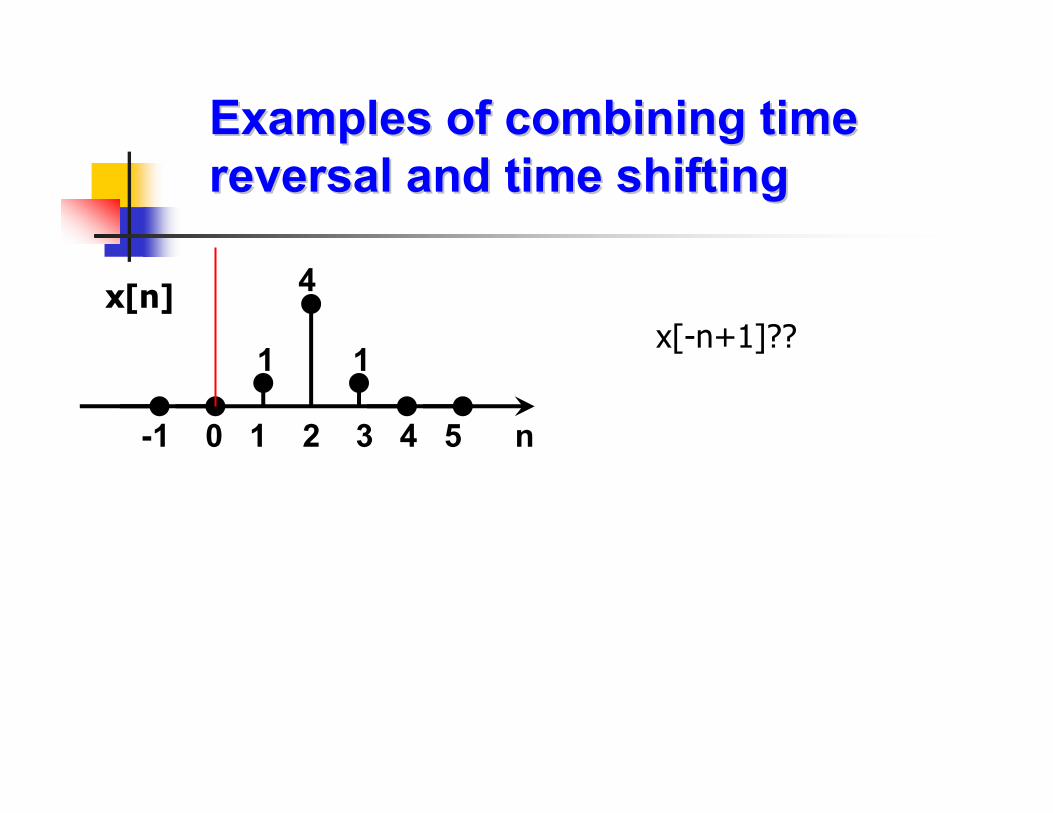
Examples of combining time Examples of combining time reversal and time shiftingreversal and time shifting
-1 0 1 2 3 4 5 n
4
1 1
x[n]x[-n+1]??

Examples of combining time Examples of combining time reversal and time shiftingreversal and time shifting
-1 0 1 2 3 4 5 n
4
1 1
x[n]x[-n-1]??
x[n] x[an-b]
Be careful!!!
To make sure, plug values into the table to check
Combining time shifting and Combining time shifting and time scalingtime scaling

Examples of combining time Examples of combining time scaling and time shiftingscaling and time shifting
-1 0 1 2 3 4 5 n
4
1 1
x[n] y[n] = x[2n-3]??
004
113
142
011
000
00-1
y[n]x[n]n
-1 0 1 2 3 4 5 n
1 1y[n]
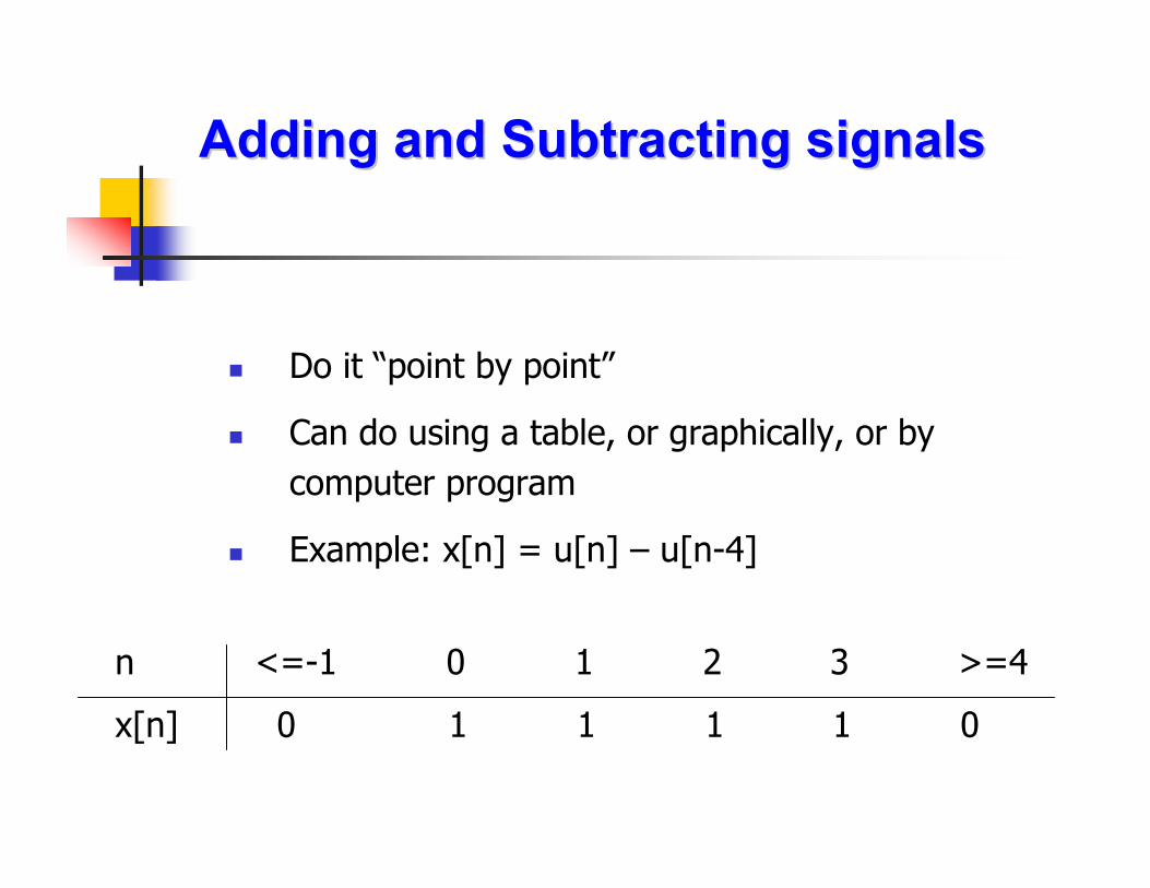
Do it “point by point”
Can do using a table, or graphically, or by
computer program
Example: x[n] = u[n] – u[n-4]
Adding and Subtracting signalsAdding and Subtracting signals
n <=-1 0 1 2 3 >=4
x[n] 0 1 1 1 1 0
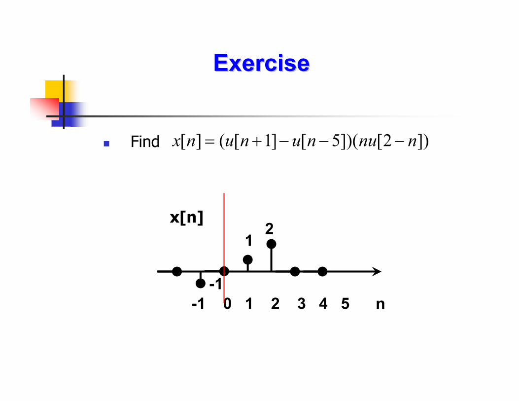
Find
ExerciseExercise
[ ] ( [ 1] [ 5])( [2 ])x n u n u n nu n= + − − −
-1 0 1 2 3 4 5 n
21
-1
x[n]
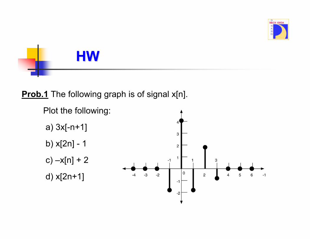
Prob.1 The following graph is of signal x[n].
Plot the following:
a) 3x[-n+1]
b) x[2n] - 1
c) –x[n] + 2
d) x[2n+1]
HWHW

Prob.2 Sometimes signals can be decomposed into combinations of
simple unit sequences such as this one:
Sketch y[n] and the following signals:
a) 2-3y[n]
b) 3y[n-2]
c) 2-2y[-2+n]
HWHW
Prob.3
Decompose y[n] from Prob. 2 into its even and odd parts. Plot
these signals and show the symmetries of the plots that can be
used to visually verify their parity
HWHW

Lecture #3Lecture #3
DT systemsDT systems
Duration: 2 hrs
Outline:
1. Input-output description of systems
2. DT system properties
3. LTI systems
Think of a DT system as an operator on DT signals:
• It processes DT input signals, to produce DT output signals
• Notation: y[n] = Tx[n] y[n] is the response of the
system T to the excitation x[n]
• Systems are assumed to be a “black box” to the user
InputInput--output description of DT systemsoutput description of DT systems

Determine the response of the following system to the unit
impulse signal
ExampleExample
............................
)8/5)(4/1(]1[2
1]2[
2
1]1[
4
1]2[
8/52/14/1]0[2
1]1[
2
1]0[
4
1]1[
2/1]1[2
1]0[
2
1]1[
4
1]0[
=++=
=+=++=
=−++−=
δδ
δδ
δδ
yy
yy
yy
]1[)8/5()4/1(][)2/1(][ 1 −+= − nunny nδ
]1n[x2
1]n[x
2
1]1n[y
4
1]n[y −++−=
• Memory
• Invertibility
• Causality
• Stability
• Linearity
• Time-invariance
DT system propertiesDT system properties
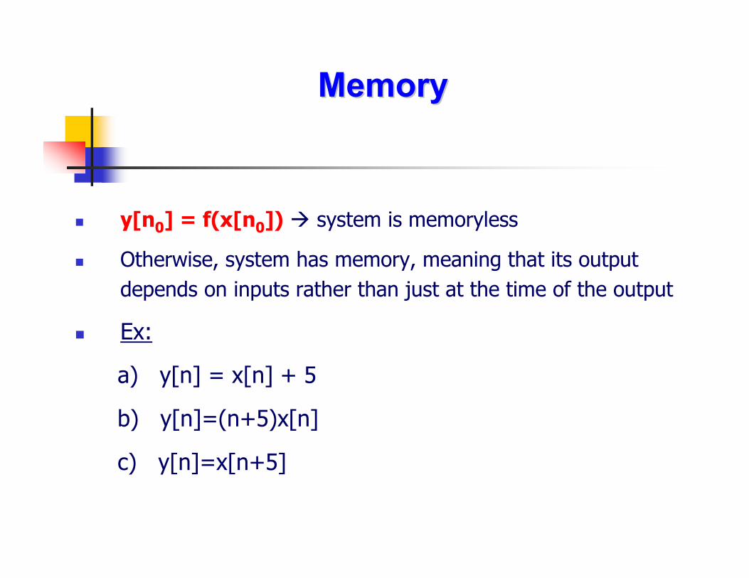
y[n0] = f(x[n0]) system is memoryless
Otherwise, system has memory, meaning that its output
depends on inputs rather than just at the time of the output
Ex:
a) y[n] = x[n] + 5
b) y[n]=(n+5)x[n]
c) y[n]=x[n+5]
MemoryMemory
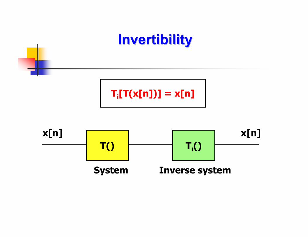
InvertibilityInvertibility
Ti[T(x[n])] = x[n]
T() Ti()
x[n] x[n]
System Inverse system

Examples for Examples for invertibilityinvertibility
Determine which of the systems below are invertible
a) Unit advance y[n] = x[n+1]
b) Accumulator
c) Rectifier y[n] = |x[n]|
∑−∞=
=n
k
kxny ][][
The output of a causal system (at each time) does not
depend on future inputs
All memoryless systems are causal
All causal systems can have memory or not
CausalityCausality

Examples for causalityExamples for causality
Determine which of the systems below are causal:
a) y[n] = x[-n]
b) y[n] = (n+1)x[n-1]
c) y[n] = x[(n-1)2]
d) y[n] = cos(w0n+x[n])
e) y[n] = 0.5y[n-1] + x[n-1]
If a system “blow up” it is not stable
In particular, if a “well-behavior” signal (all values have
finite amplitude) results in infinite magnitude outputs,
the system is unstable
BIBO stability: “bounded input – bounded output” –
if you put finite signals in, you will get finite signals out
StabilityStability

Examples for stabilityExamples for stability
Determine which of the systems below are BIBO stable:
a) A unit delay system
b) An accumulator
c) y[n] = cos(x[n])
d) y[n] = ln(x[n])
e) y[n] =exp(x[n])

Scaling signals and adding them, then processing through the system
same as
Processing signals through system, then scaling and adding them
LinearityLinearity
If T(x1[n]) = y1[n] and T(x2[n]) = y2[n]
T(ax1[n] + bx2[n]) = ay1[n] + by2[n]
If you time shift the input, get the same output, but with the
same time shift
The behavior of the system doesn’t change with time
TimeTime--invarianceinvariance
If T(x[n]) = y[n]
then T(x[n-n0]) = y[n-n0]

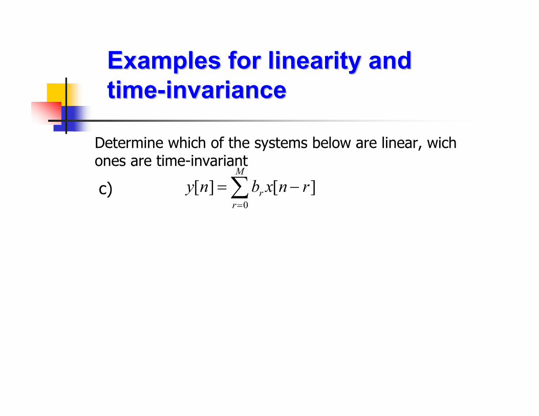
Examples for linearity and Examples for linearity and timetime--invarianceinvariance
Determine which of the systems below are linear, wichones are time-invariant
a) [ ] [ ]y n nx n=
Examples for linearity and Examples for linearity and timetime--invarianceinvariance
Determine which of the systems below are linear, wichones are time-invariant
b) ]n[x]n[y 2=
Examples for linearity and Examples for linearity and timetime--invarianceinvariance
Determine which of the systems below are linear, wichones are time-invariant
c) ∑=
−=M
r
r rnxbny0
][][

Prob.4 Which systems are linear? Which ones are time-invariant?
HWHW
∑
∑
=
−∞=
=
=
=
=
+Ω=
=
n
k
n
k
kxnyf
kxnye
nunxnyd
nxnyc
nxnnyb
nxnya
0
0
][][)
][][)
][][][)
]2[][)
])[cos(][)
])[sin(][)

Prob.5 For the following systems:
Prove or disprove that they are:
Memoryless
Invertible
Causal
Stable
Time-invariant
Linear
HWHW
Ζ∈−=
−+=
=
Ζ∈+=
∑
∑
−
−=
−=
Mknxnyd
nxnxnyc
exnyb
akaxnya
M
k
n
n
nk
,][][)
]1[5.0][5.0][)
)(][)
,][][)
1
0
||

Method 1: based on the direct solution of the input-output equation
for the system
Method 2:
• Decompose the input signal into a sum of elementary signals
• Find the response of system
to each elementary signal
• Add those responses to obtain
the total response of the system
to the given input signal
Computing the response of DT LTI Computing the response of DT LTI systems to arbitrary inputssystems to arbitrary inputs
∑
∑
=→
→
=
k
kk
kk
k
kk
nycnynx
nynx
nxcnx
][][][
][][
][][
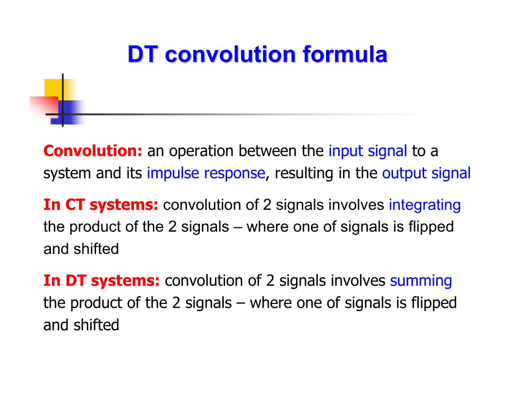
Convolution: an operation between the input signal to a
system and its impulse response, resulting in the output signal
In CT systems: convolution of 2 signals involves integrating
the product of the 2 signals – where one of signals is flipped
and shifted
In DT systems: convolution of 2 signals involves summing
the product of the 2 signals – where one of signals is flipped
and shifted
DT convolution formulaDT convolution formula

We can describe any DT signal x[n] as:
Example:
Impulse representation of DT Impulse representation of DT signalssignals
[ ] [ ] [ ]k
x n x k n kδ∞
=−∞
= −∑
-1 0 1 2 3 n
x[n]
-1 0 1 2 n
x[0]δ[n-0]
-1 0 1 2 n
x[1]δ[n-1]
-1 0 1 2 n
x[2]δ[n-2]+ +

Impulse response: the output results, in response to a unit
impulse
Denotation: hk[n]: impulse response of a system, to an impulse
at time k
Impulse response of DT systemsImpulse response of DT systems
Time-invariant DT system
Time-invariant DT system
δ[n]
δ[n-k]
h[n]
h[n-k]
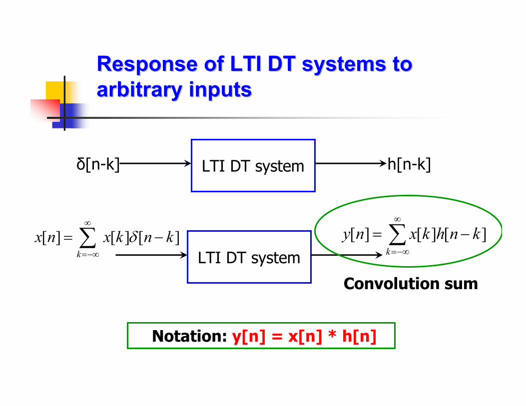
Response of LTI DT systems to Response of LTI DT systems to arbitrary inputsarbitrary inputs
LTI DT systemδ[n-k] h[n-k]
LTI DT system
[ ] [ ] [ ]k
x n x k n kδ∞
=−∞
= −∑ ∑∞
−∞=
−=k
knhkxny ][][][
Notation: y[n] = x[n] * h[n]
Convolution sum
Commutative law
Associative law
Distributive law
Convolution sum propertiesConvolution sum properties

Commutative lawCommutative law
][*][][*][ nxnhnhnx =
h[n]x[n] y[n]
x[n]h[n] y[n]
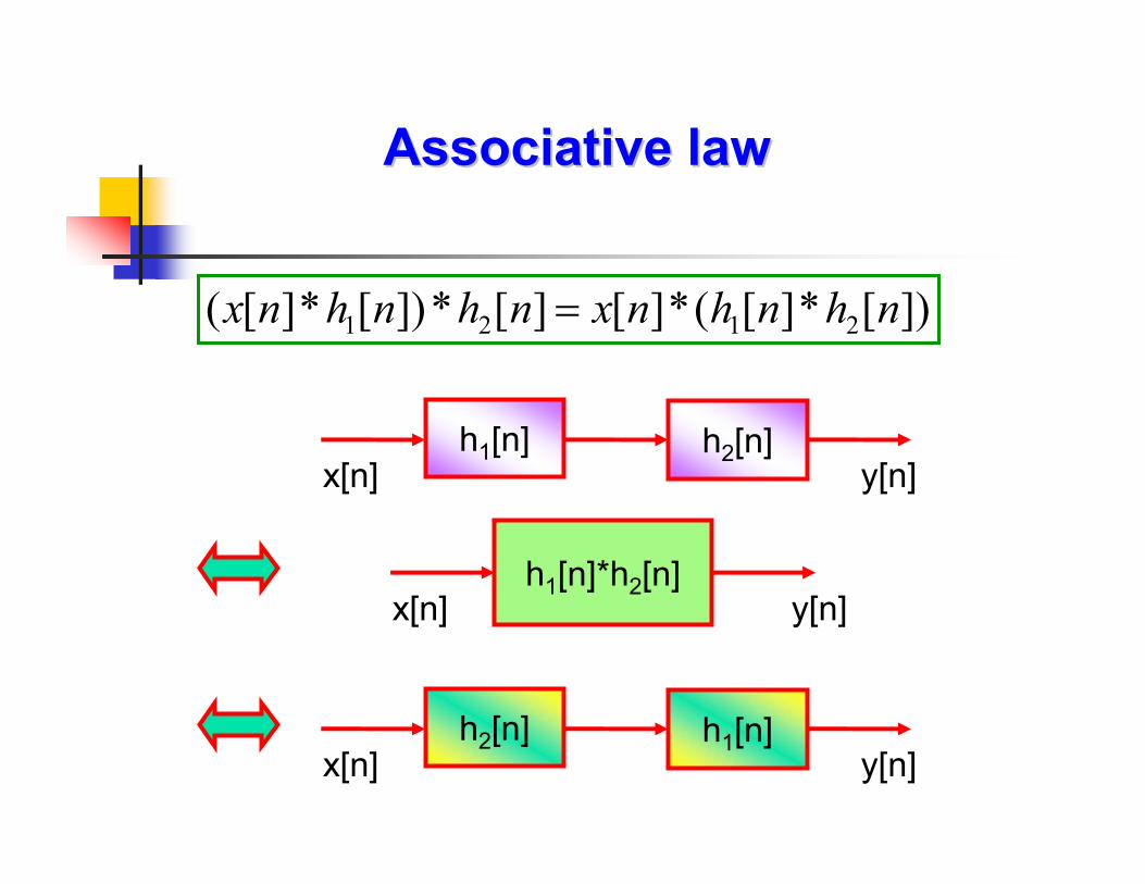
Associative lawAssociative law
])[*][(*][][*])[*][( 2121 nhnhnxnhnhnx =
h1[n]x[n] y[n]
h2[n]
h2[n]x[n] y[n]
h1[n]
h1[n]*h2[n]x[n] y[n]

Distributive lawDistributive law
])[*][(])[*][(])[][(*][ 2121 nhnxnhnxnhnhnx +=+
h1[n] + h2[n]x[n] y[n]
h1[n]
x[n] y[n]
h2[n]
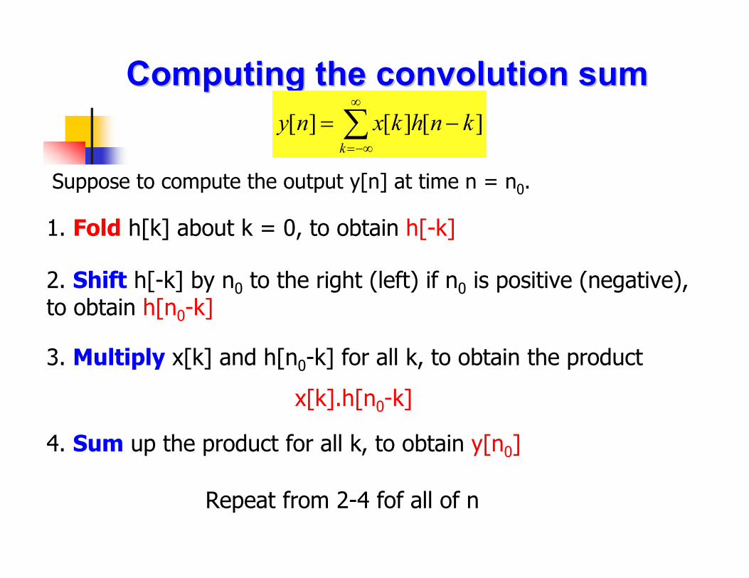
Computing the convolution sumComputing the convolution sum
Suppose to compute the output y[n] at time n = n0.
1. Fold h[k] about k = 0, to obtain h[-k]
2. Shift h[-k] by n0 to the right (left) if n0 is positive (negative), to obtain h[n0-k]
3. Multiply x[k] and h[n0-k] for all k, to obtain the product
x[k].h[n0-k]
4. Sum up the product for all k, to obtain y[n0]
Repeat from 2-4 fof all of n
∑∞
−∞=
−=k
knhkxny ][][][

The length of the convolution The length of the convolution sum resultsum result
Suppose:
Length of x[k] is Nx N1 ≤ k ≤ N1 + Nx – 1
Length of h[n-k] is Nh N2 ≤ n-k ≤ N2 + Nh – 1
N1 + N2 ≤ n ≤ N1 + N2 + Nx + Nh – 2
Length of y[n]:
Ny = Nx + Nh – 1
[ ] [ ] [ ] [ ] [ ]k
y n x n h n x k h n k∞
=−∞
= ∗ = −∑
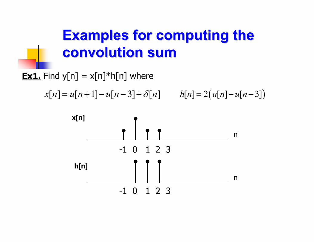
Examples for computing the Examples for computing the convolution sumconvolution sum
Ex1. Find y[n] = x[n]*h[n] where
[ ] [ 1] [ 3] [ ]x n u n u n nδ= + − − + ( )[ ] 2 [ ] [ 3]h n u n u n= − −
n
n
x[n]
h[n]
-1 0 1 2 3
-1 0 1 2 3
h[-k]h[k]
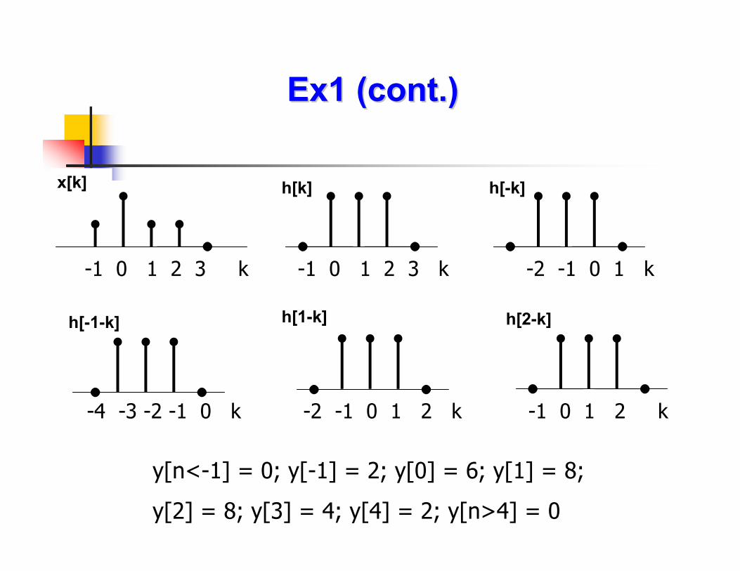
Ex1 (cont.)Ex1 (cont.)
x[k]
-1 0 1 2 3 k -1 0 1 2 3 k -2 -1 0 1 k
-4 -3 -2 -1 0 k
h[2-k]
-1 0 1 2 k
h[-1-k] h[1-k]
-2 -1 0 1 2 k
y[n<-1] = 0; y[-1] = 2; y[0] = 6; y[1] = 8;
y[2] = 8; y[3] = 4; y[4] = 2; y[n>4] = 0

Examples for computing the Examples for computing the convolution sumconvolution sum
Ex2. Find y[n] = x[n]*h[n] where [ ] [ ]nx n a u n= [ ] [ ]h n u n=
1. Do it graphically
2. Use convolution formula

Examples for computing the Examples for computing the convolution sumconvolution sum
Ex3. Find y[n] = x[n]*h[n] where x[n] = bnu[n] and h[n] = anu[n+2]
|a| < 1, |b| < 1, a ≠ b
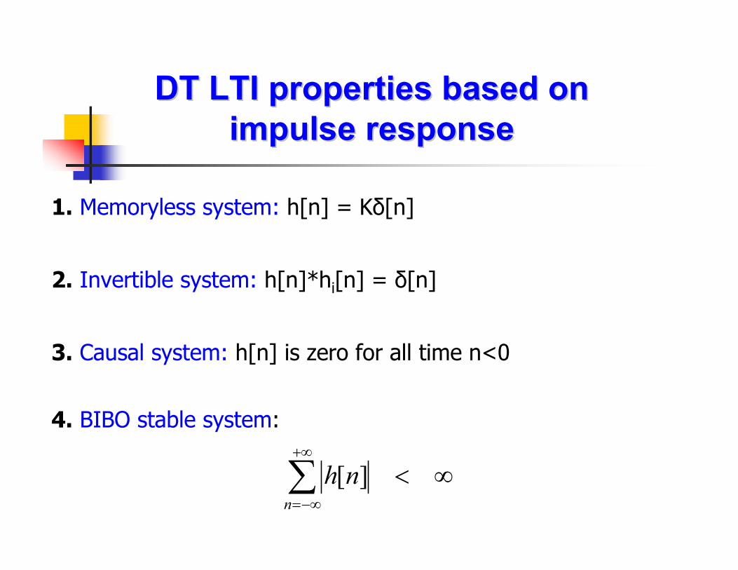
DT LTI properties based on DT LTI properties based on impulse responseimpulse response
1. Memoryless system: h[n] = Kδ[n]
2. Invertible system: h[n]*hi[n] = δ[n]
3. Causal system: h[n] is zero for all time n<0
4. BIBO stable system:
∞<∑+∞
−∞=n
nh ][

Examples of DT LTI propertiesExamples of DT LTI properties
1. What is the inverse of h[n] = 3δ[n+5]?
2. Is h[n] = 0.5nu[n] BIBO stable? Causal?
3. Is h[n] = 3nu[n] BIBO stable? Causal?
4. Is h[n] = 3nu[-n] BIBO stable? Causal?
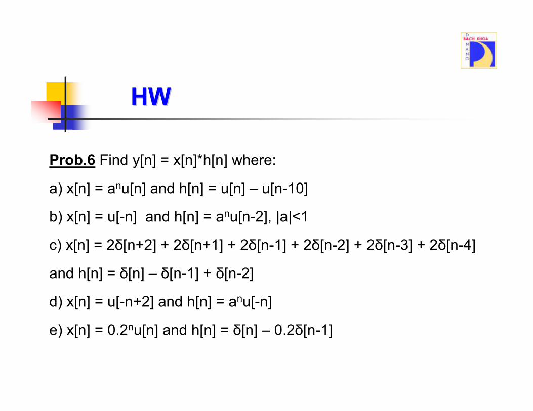
Prob.6 Find y[n] = x[n]*h[n] where:
a) x[n] = anu[n] and h[n] = u[n] – u[n-10]
b) x[n] = u[-n] and h[n] = anu[n-2], |a|<1
c) x[n] = 2δ[n+2] + 2δ[n+1] + 2δ[n-1] + 2δ[n-2] + 2δ[n-3] + 2δ[n-4]
and h[n] = δ[n] – δ[n-1] + δ[n-2]
d) x[n] = u[-n+2] and h[n] = anu[-n]
e) x[n] = 0.2nu[n] and h[n] = δ[n] – 0.2δ[n-1]
HWHW
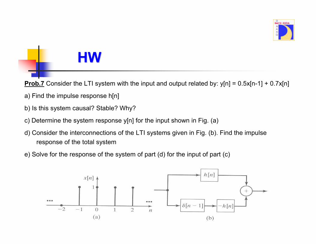
Prob.7 Consider the LTI system with the input and output related by: y[n] = 0.5x[n-1] + 0.7x[n]
a) Find the impulse response h[n]
b) Is this system causal? Stable? Why?
c) Determine the system response y[n] for the input shown in Fig. (a)
d) Consider the interconnections of the LTI systems given in Fig. (b). Find the impulse
response of the total system
e) Solve for the response of the system of part (d) for the input of part (c)
HWHW
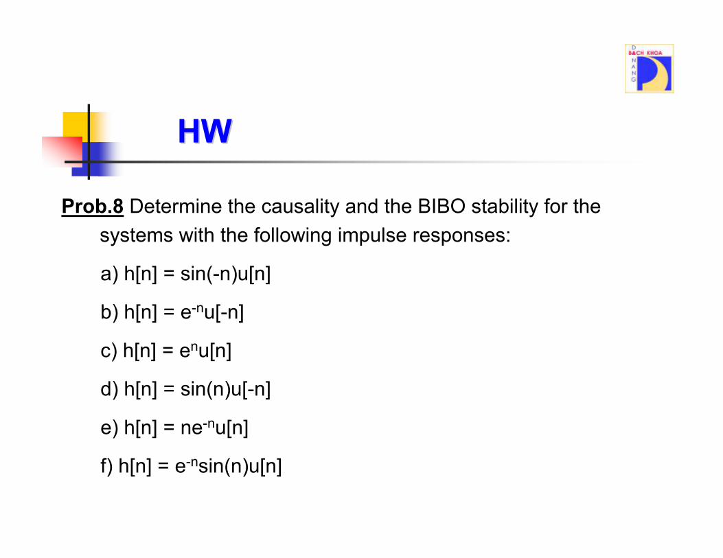
Prob.8 Determine the causality and the BIBO stability for the
systems with the following impulse responses:
a) h[n] = sin(-n)u[n]
b) h[n] = e-nu[-n]
c) h[n] = enu[n]
d) h[n] = sin(n)u[-n]
e) h[n] = ne-nu[n]
f) h[n] = e-nsin(n)u[n]
HWHW
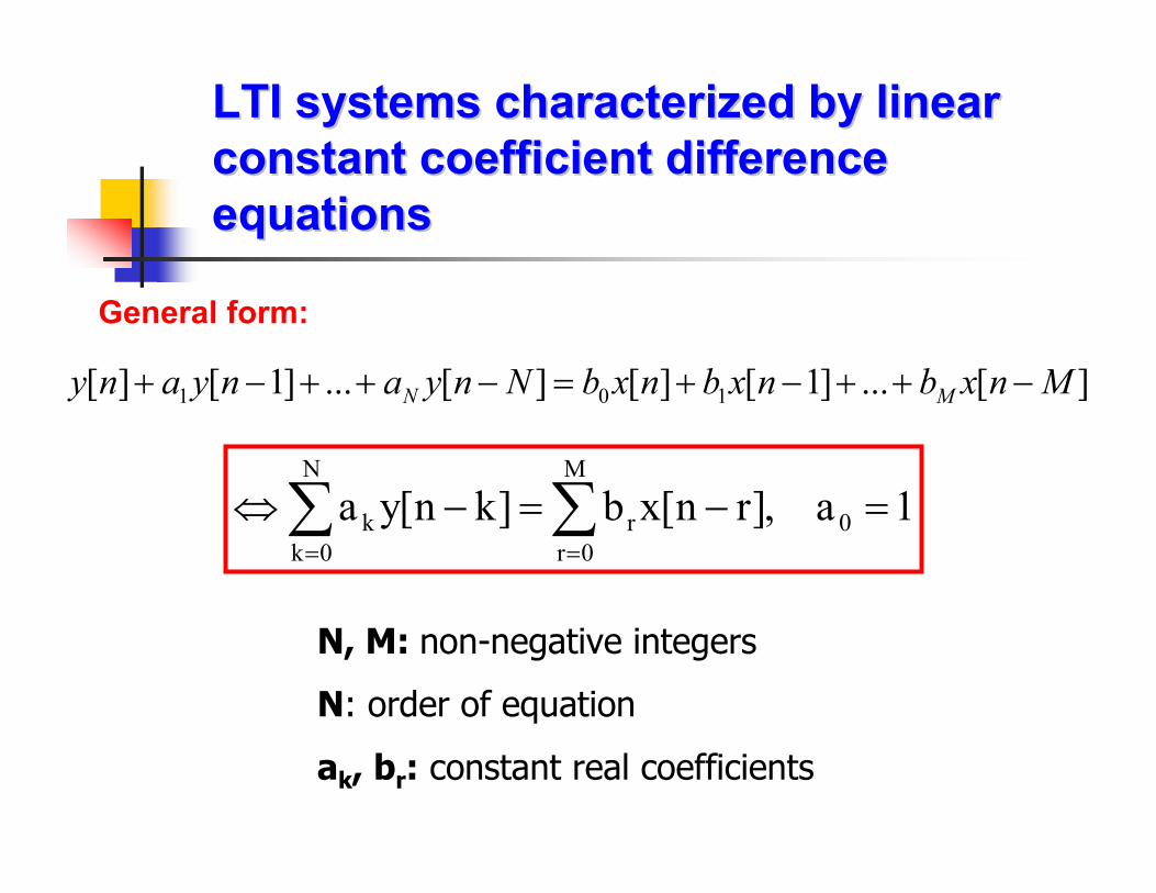
General form:
LTI systems characterized by linear LTI systems characterized by linear constant coefficient difference constant coefficient difference equationsequations
][...]1[][][...]1[][ 101 Mnxbnxbnxbnyanyany M −++−+=−++−+
1a,]rn[xb]kn[ya 0
M
0r
r
N
0k
k =−=−⇔ ∑∑==
N, M: non-negative integers
N: order of equation
ak, br: constant real coefficients
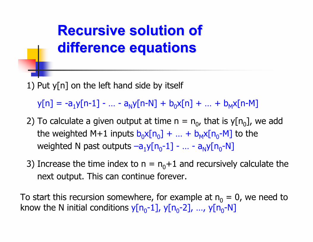
1) Put y[n] on the left hand side by itself
y[n] = -a1y[n-1] - … - aNy[n-N] + b0x[n] + … + bMx[n-M]
2) To calculate a given output at time n = n0, that is y[n0], we add
the weighted M+1 inputs b0x[n0] + … + bMx[n0-M] to the
weighted N past outputs –a1y[n0-1] - … - aNy[n0-N]
3) Increase the time index to n = n0+1 and recursively calculate the
next output. This can continue forever.
Recursive solution of Recursive solution of difference equationsdifference equations
To start this recursion somewhere, for example at n0 = 0, we need to know the N initial conditions y[n0-1], y[n0-2], …, y[n0-N]
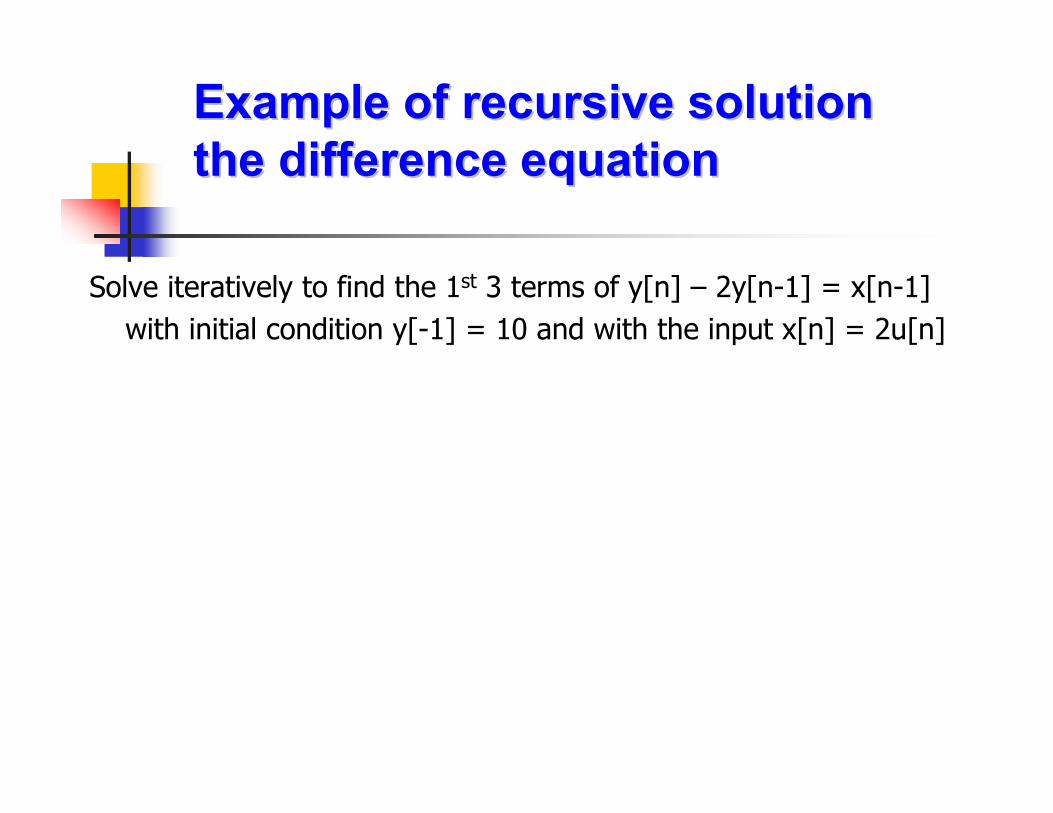
Solve iteratively to find the 1st 3 terms of y[n] – 2y[n-1] = x[n-1]
with initial condition y[-1] = 10 and with the input x[n] = 2u[n]
Example of recursive solution Example of recursive solution the difference equationthe difference equation
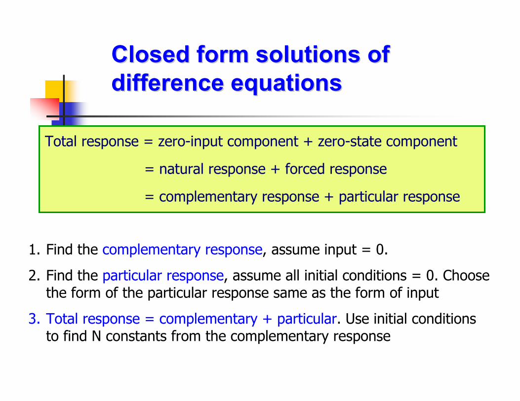
Total response = zero-input component + zero-state component
= natural response + forced response
= complementary response + particular response
Closed form solutions of Closed form solutions of difference equationsdifference equations
1. Find the complementary response, assume input = 0.
2. Find the particular response, assume all initial conditions = 0. Choose the form of the particular response same as the form of input
3. Total response = complementary + particular. Use initial conditions to find N constants from the complementary response
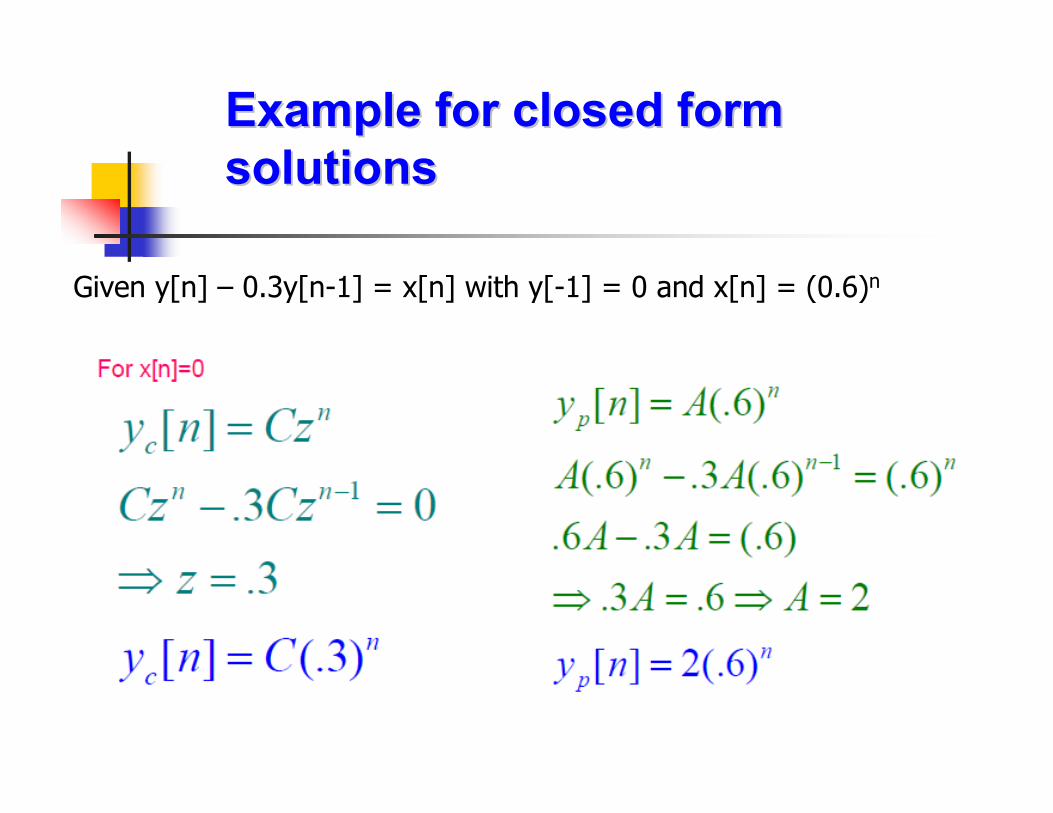
Example for closed form Example for closed form solutionssolutions
Given y[n] – 0.3y[n-1] = x[n] with y[-1] = 0 and x[n] = (0.6)n

Example (cont)Example (cont)
Combining particular and complementary solutions:

Prob.9 Determine the response y[n] for n≥0 of the system
described by the following equation:
y[n] -0.7y[n-1] + 0.1y[n-2] = x[n] – 3x[n-1]
The input is x[n] = (-1)n and y[-2] = 29/9, y[-1] = 7/9
HWHW