chapter10 image segmentation
TRANSCRIPT
Image Segmentation
Subject: FIP (181102)
Prof. Asodariya Bhavesh
ECD,SSASIT, Surat
Image Segmentation
• Image segmentation divides an image into regions that are connected and have some similarity within the region and some difference between adjacent regions.
• The goal is usually to find individual objects in an image.• For the most part there are fundamentally two kinds of
approaches to segmentation: discontinuity and similarity. – Similarity may be due to pixel intensity, color or texture. – Differences are sudden changes (discontinuities) in any of these, but
especially sudden changes in intensity along a boundary line, which is called an edge.
Detection of Discontinuities
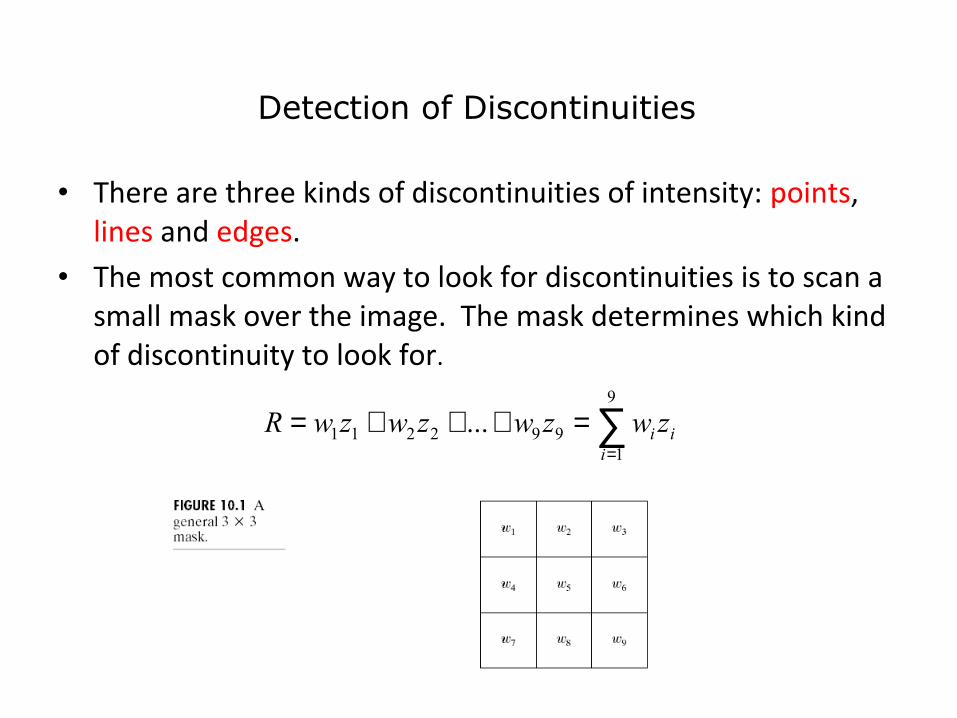
• There are three kinds of discontinuities of intensity: points, lines and edges.
• The most common way to look for discontinuities is to scan a small mask over the image. The mask determines which kind of discontinuity to look for.
∑=
=+++=9
1992211 ...
iii zwzwzwzwR
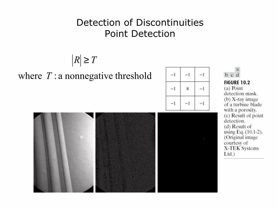
Detection of DiscontinuitiesPoint Detection
thresholdenonnegativ a: where T
TR ≥

Detection of DiscontinuitiesLine Detection
• Only slightly more common than point detection is to find a one pixel wide line in an image.
• For digital images the only three point straight lines are only horizontal, vertical, or diagonal (+ or –45°).

Detection of DiscontinuitiesLine Detection
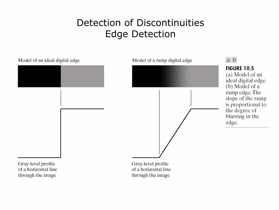
Detection of DiscontinuitiesEdge Detection
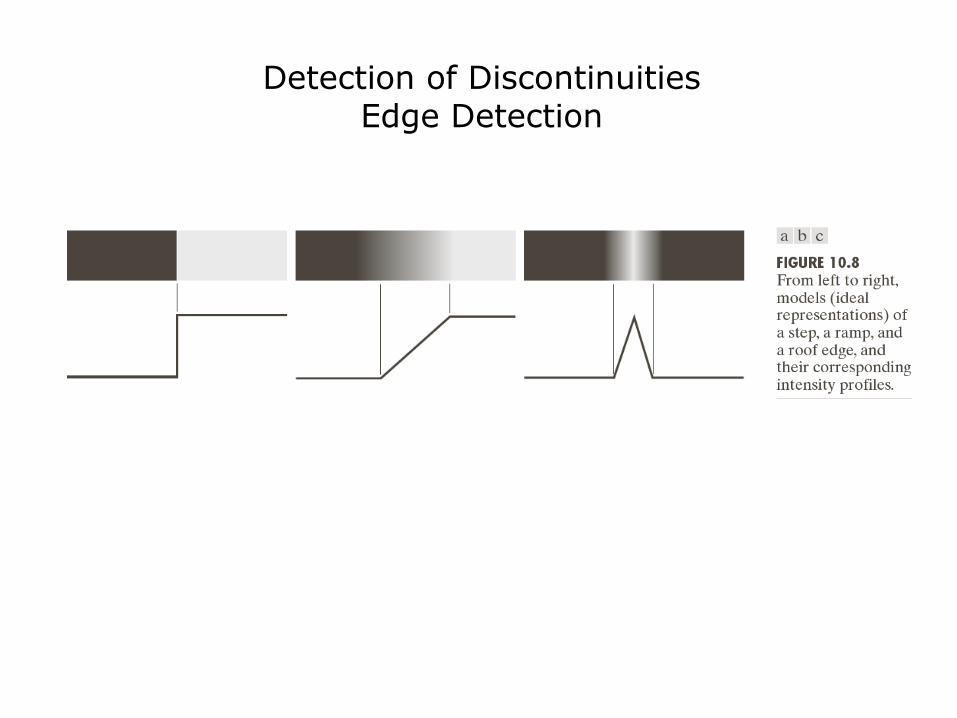
Detection of DiscontinuitiesEdge Detection
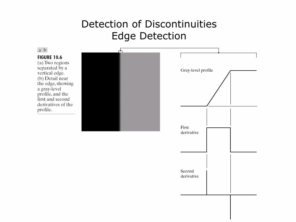
Detection of DiscontinuitiesEdge Detection
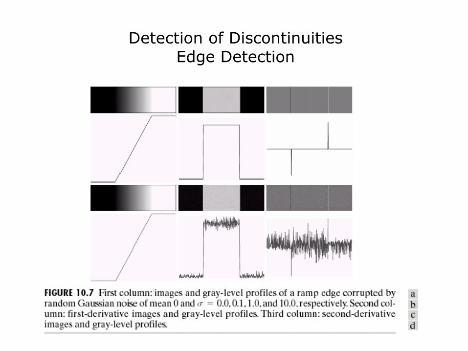
Detection of DiscontinuitiesEdge Detection
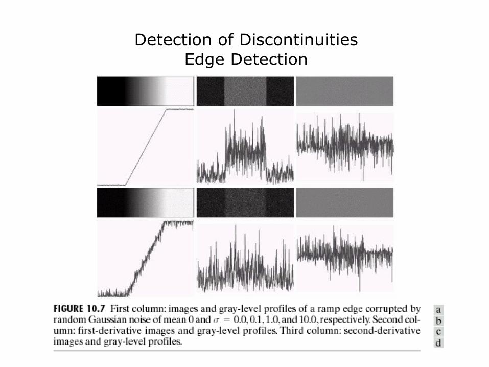
Detection of DiscontinuitiesEdge Detection

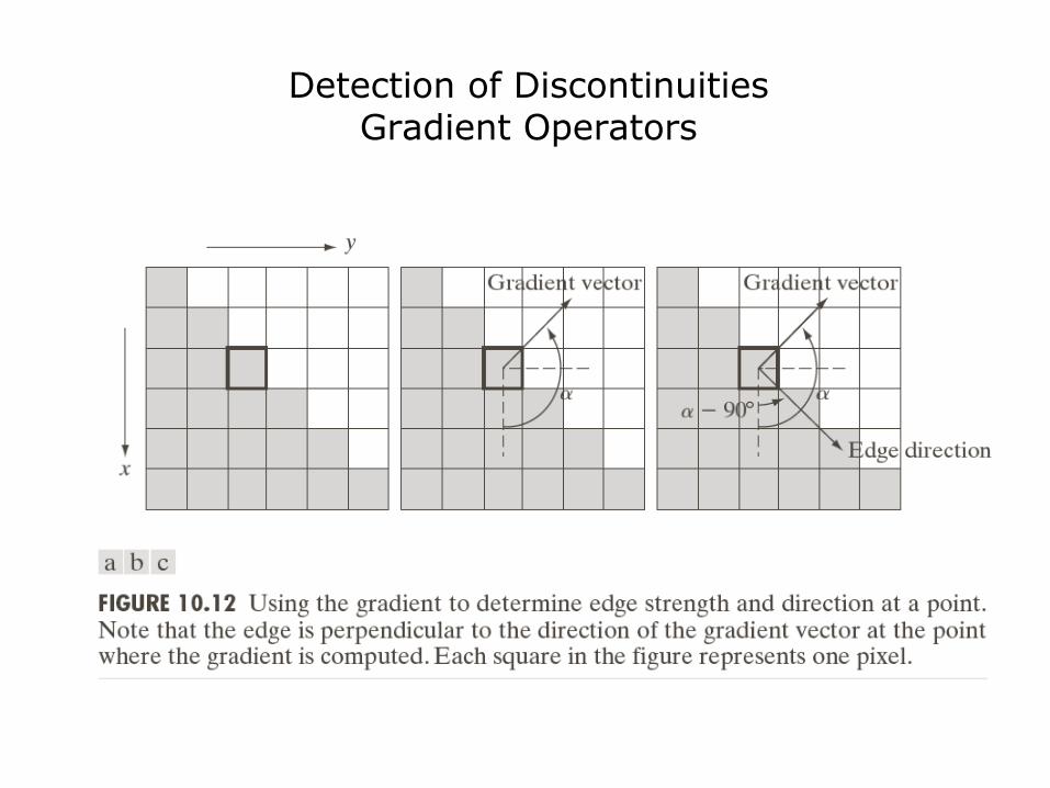
Detection of DiscontinuitiesGradient Operators
• First-order derivatives:– The gradient of an image f(x,y) at location (x,y) is
defined as the vector:
– The magnitude of this vector:
– The direction of this vector:
– It points in the direction of the greatest rate of change of f at location (x,y)
=
=∇
∂∂∂∂
yfxf
y
x
G
Gf
[ ] 21
22)(mag yx GGf +=∇=∇ f
= −
y
x
G
Gyx 1tan),(α
Detection of DiscontinuitiesGradient Operators

Detection of DiscontinuitiesGradient Operators
Roberts cross-gradient operators
Prewitt operators
Sobel operators
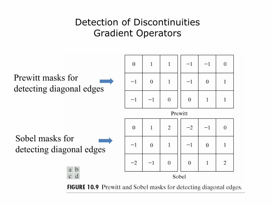
Detection of DiscontinuitiesGradient Operators
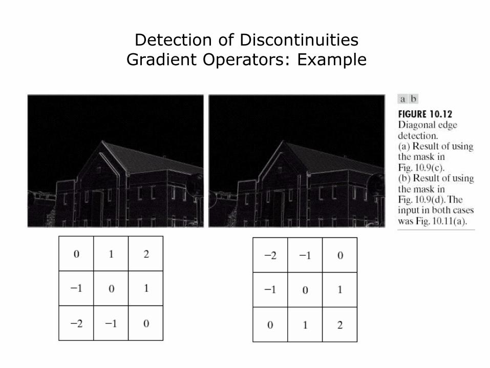
Prewitt masks for detecting diagonal edges
Sobel masks for detecting diagonal edges
yx GGf +≈∇
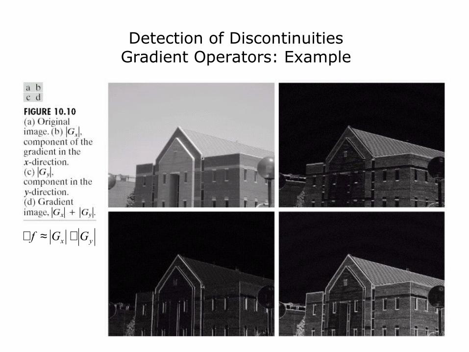
Detection of DiscontinuitiesGradient Operators: Example

Detection of DiscontinuitiesGradient Operators: Example
Detection of DiscontinuitiesGradient Operators: Example

Detection of DiscontinuitiesGradient Operators: Example
Detection of DiscontinuitiesGradient Operators
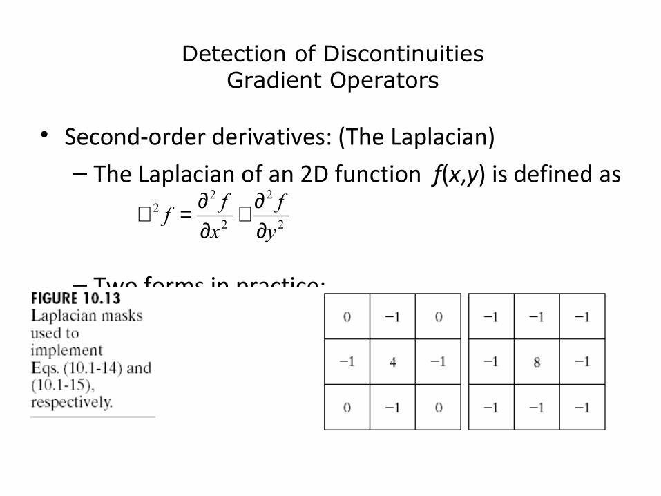
• Second-order derivatives: (The Laplacian)– The Laplacian of an 2D function f(x,y) is defined as
– Two forms in practice:
2
2
2
22
y
f
x
ff
∂∂+
∂∂=∇
More Advanced Techniques for Edge Detection
Marr-Hildreth edge detectorMarr and Hildreth argued that
1) Intensity changes are dependent of image scale and so their detection requires the use of operators different sizes and2) That a sudden intensity change will give rise to a peak or trough in the first derivative or, equivalently, to zero crossing in the second derivative.Two salient feature:1)It should be differential operator capable of computing first or second order derivatives at every point in an image2)It should be capable of being tuned to act at any desired scale, so that large operator can be used to detect blurry edges and small operators to detect sharply focused fine detail

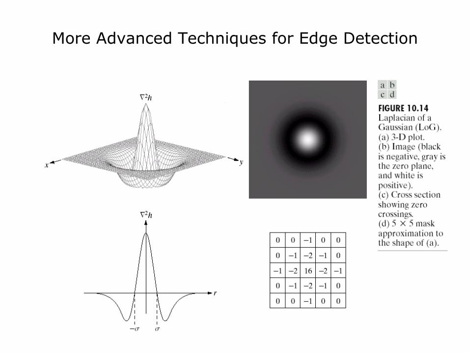
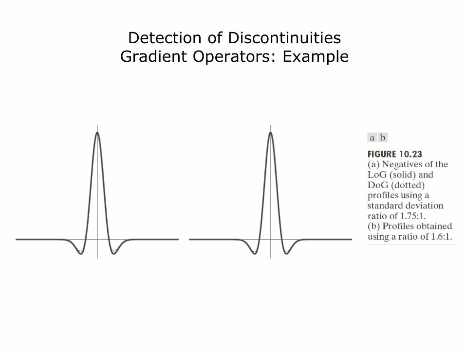
• Consider the function:
• The Laplacian of h is
• The Laplacian of a Gaussian sometimes is called the Mexican hat function. It also can be computed by smoothing the image with the Gaussian smoothing mask, followed by application of the Laplacian mask.
deviation standard the: and
where)( 2222 2
2
σ
σ yxrerhr
+=−=−
2
2
24
222 )( σ
σσ r
er
rh−
−−=∇The Laplacian of a
Gaussian (LoG)
A Gaussian function
More Advanced Techniques for Edge Detection

• Marr-Hildreth edge detector• Marr and Hildreth argued that the most satisfactory operator fulfilling these
conditions is the filter ∇2G where, ∇2 is the Laplacian operator, and G is the 2-D Gaussian function
(LoG)Gaussion a ofLaplacian called is expression This
2),(
11),(
),(
),(),(),(
),(
2
22
2
22
2
22
2
22
2
22
2
22
24
2222
224
22
24
22
22
22
2
2
2
2
22
2
σ
σσ
σσ
σ
σσ
σσσσ
σσ
yx
yxyx
yxyx
yx
eyx
yxG
ey
ex
yxG
ey
ye
x
xyxG
y
yxG
x
yxGyxG
eyxG
+−
+−+−
+−+−
+−
−+=∇
−+
−=∇
−∂∂+
−∂∂=∇
∂∂+
∂∂=∇
=
More Advanced Techniques for Edge Detection
More Advanced Techniques for Edge Detection
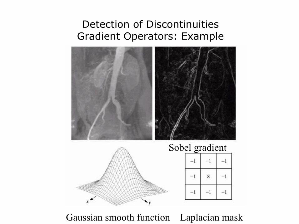
Detection of DiscontinuitiesGradient Operators: Example
Sobel gradient
Laplacian maskGaussian smooth function
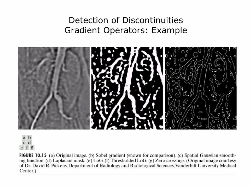
Detection of DiscontinuitiesGradient Operators: Example
Detection of DiscontinuitiesGradient Operators: Example

Hough Transforms
Hough Transforms takes the images created by the edge detection operatorsMost of the time, the edge map generated by the edge detection algorithms is disconnectedHT can be used to connect the disjointed edge pointsIt is used to fit the points as plane curvesPlane curves are lines, circles, and parabolas
The line equation is y = mx + cHowever, the problem is that there are infinite line passing through one pointsTherefore, an edge point in an x-y plane is transformed to a c-m planeNow equation of line is c = (-x)m + y

Hough Transforms
All the edge points in the x-y plane need to be fittedAll the points are transformed in c-m planeThe objective is to find the intersection pointA common intersection point indicates that the edges points which are part of the lineIf A and B are the points connected by a line in the spatial domain, then they will be intersecting lines in the Hough Space (c-m plane)To check whether they are intersecting lines, the c-m plane is partitioned as accumulator linesTo find this, it can be assumed that the c-m plane can be partitioned as an accumulator arrayFor every edge point (x,y), the corresponding accumulator element is incremented in the accumulator arrayAt the end of this process, the accumulator values are checkedSignificance is that this point gives us the line equation of the (x,y) space

Hough Transforms
Hough Transform steps:1)Load the image2)Find the edges of the image using any edge detector3)Quantize the parameter space P4)Repeat the following for all the pixels of the image:
if the pixel is an edge pixel, then(a) c = (-x)m + y or calculate ρ(b) P(c,m) = P(c,m) + 1 or increment position in P
5)Show the Hough Space6)Find the local maxima in the parameter space7)Draw the line using the local maxima The major problem with this algorithm is that it does not work for vertical lines, as they have a slope of infinityConvert line into polar coordinates ρ = x cosӨ + ysinӨ, where Ө is the angle between the line and x-axis, and ρ is the diameter
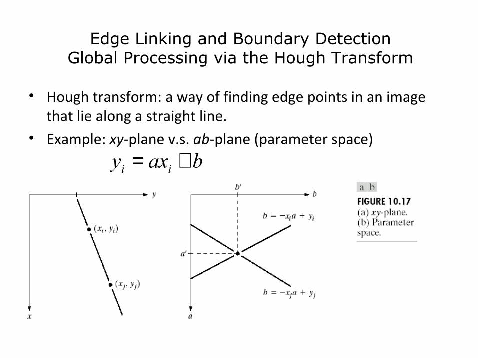
Edge Linking and Boundary DetectionGlobal Processing via the Hough Transform
• Hough transform: a way of finding edge points in an image that lie along a straight line.
• Example: xy-plane v.s. ab-plane (parameter space)
baxy ii +=
Edge Linking and Boundary DetectionGlobal Processing via the Hough Transform
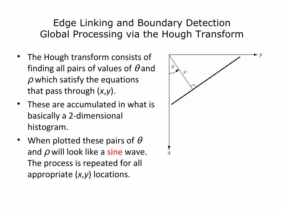
• The Hough transform consists of finding all pairs of values of θ and ρ which satisfy the equations that pass through (x,y).
• These are accumulated in what is basically a 2-dimensional histogram.
• When plotted these pairs of θ and ρ will look like a sine wave. The process is repeated for all appropriate (x,y) locations.
ρθθ =+ sincos yx

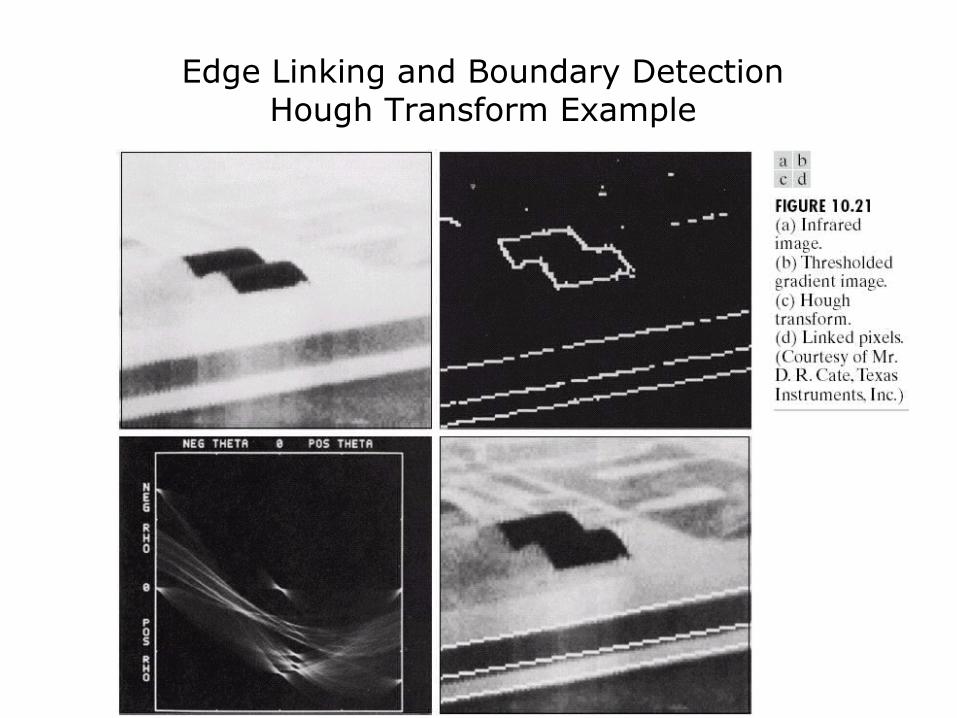
Edge Linking and Boundary DetectionHough Transform Example
The intersection of the curves corresponding
to points 1,3,5
2,3,4
1,4

Edge Linking and Boundary DetectionHough Transform Example
Thresholding
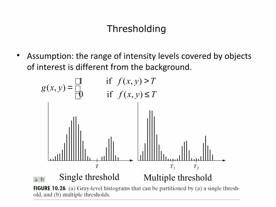
• Assumption: the range of intensity levels covered by objects of interest is different from the background.
≤>
=Tyxf
Tyxfyxg
),( if 0
),( if 1),(
Single threshold Multiple threshold
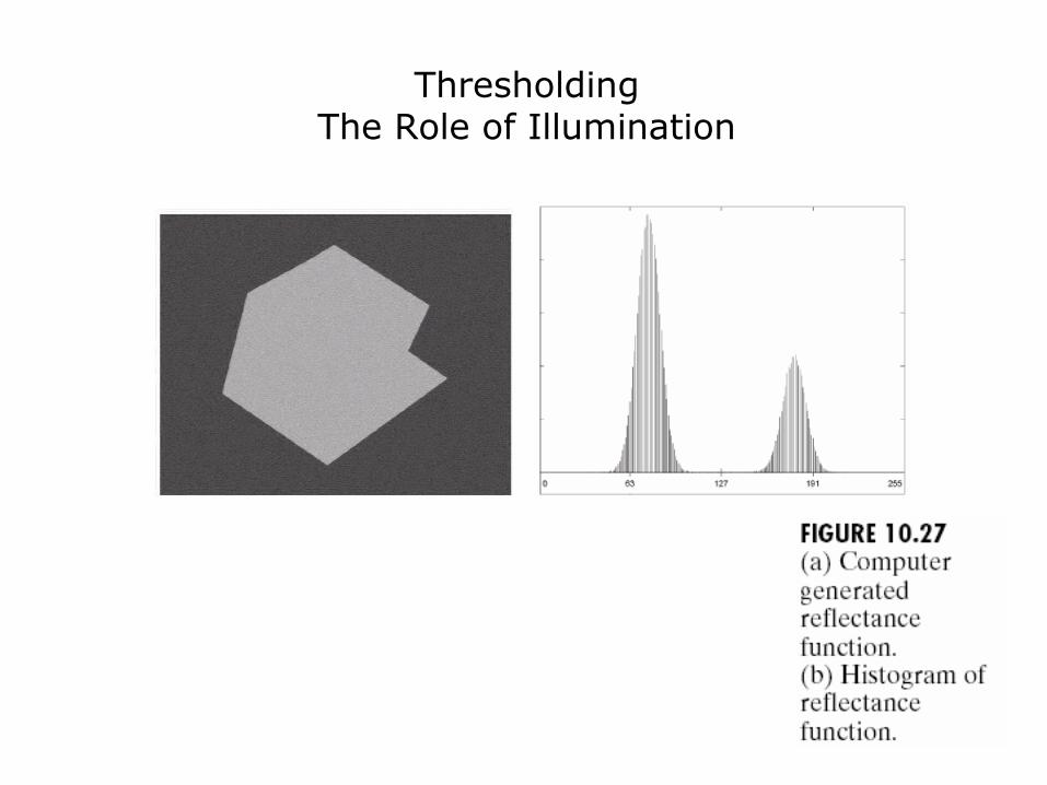
ThresholdingThe Role of Illumination
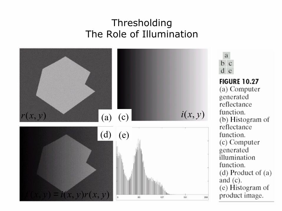
ThresholdingThe Role of Illumination
(a) (c)
(e)(d)
),(),(),( yxryxiyxf =
),( yxi),( yxr
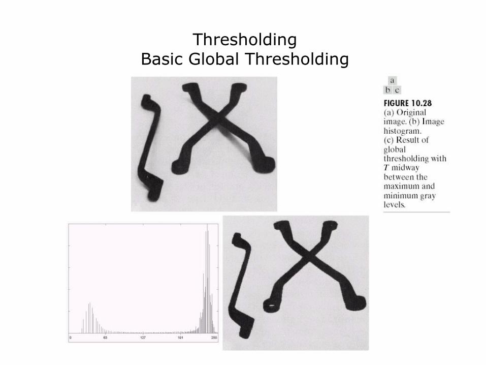
ThresholdingBasic Global Thresholding

ThresholdingBasic Global Thresholding
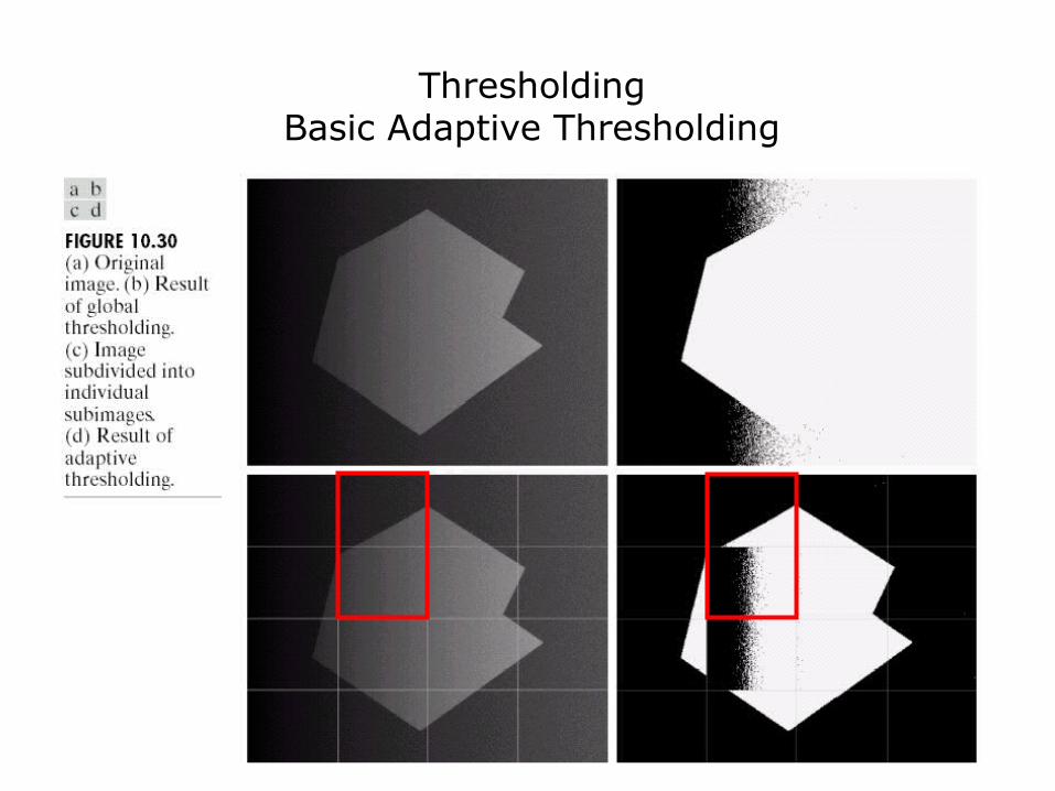
ThresholdingBasic Adaptive Thresholding
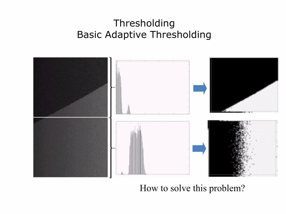
ThresholdingBasic Adaptive Thresholding
How to solve this problem?
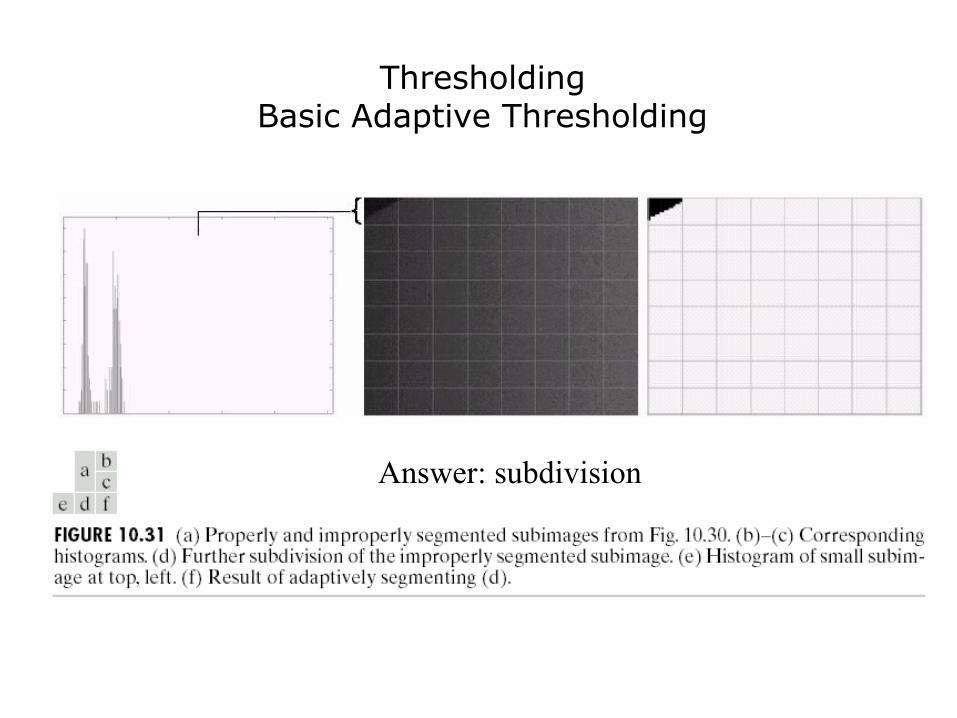
ThresholdingBasic Adaptive Thresholding
Answer: subdivision
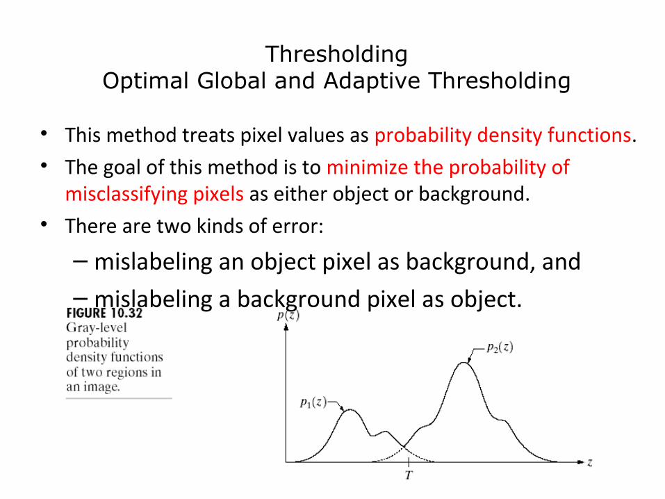
ThresholdingOptimal Global and Adaptive Thresholding
• This method treats pixel values as probability density functions. • The goal of this method is to minimize the probability of
misclassifying pixels as either object or background. • There are two kinds of error:
– mislabeling an object pixel as background, and– mislabeling a background pixel as object.

ThresholdingUse of Boundary Characteristics

ThresholdingThresholds Based on Several Variables
Color image

Region-Based Segmentation
• Edges and thresholds sometimes do not give good results for segmentation.
• Region-based segmentation is based on the connectivity of similar pixels in a region.– Each region must be uniform. – Connectivity of the pixels within the region is very
important. • There are two main approaches to region-based
segmentation: region growing and region splitting.

Region-Based SegmentationBasic Formulation
• Let R represent the entire image region.• Segmentation is a process that partitions R into subregions,
R1,R2,…,Rn, such that
where P(Rk): a logical predicate defined over the points in set Rk
For example: P(Rk)=TRUE if all pixels in Rk have the same gray level.
RRin
i=∪
=1 (a)
jijiRR ji ≠=∩ , and allfor (c) φniRi ,...,2,1 region, connected a is (b) =
niRP i ,...,2,1for TRUE)( (d) ==
jiji RRRRP and regionsadjacent any for FALSE)( (e) =∪

Region Growing
• Thresholding still produces isolated image
• Region growing algorithms works on principle of similarity
• It states that a region is coherent if all the pixels of that region are homogeneous with respect to some characteristics such as colour, intensity, texture, or other statistical properties
• Thus idea is to pick a pixel inside a region of interest as a starting point (also known as a seed point) and allowing it to grow
• Seed point is compared with its neighbours, and if the properties match , they are merged together
• This process is repeated till the regions converge to an extent that no further merging is possible
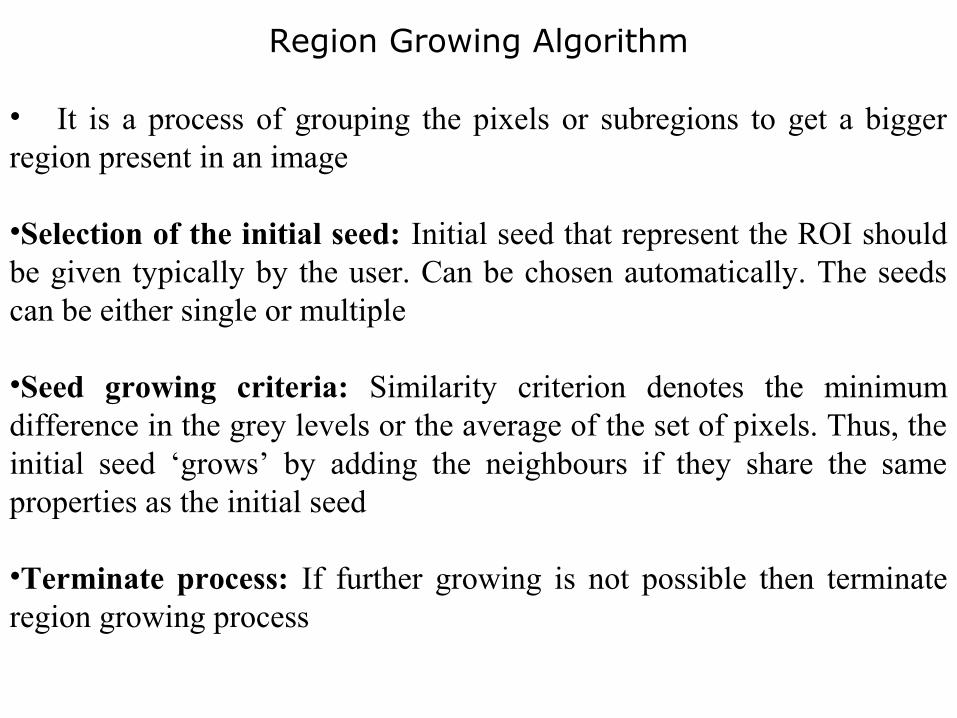
Region Growing Algorithm
• It is a process of grouping the pixels or subregions to get a bigger region present in an image
•Selection of the initial seed: Initial seed that represent the ROI should be given typically by the user. Can be chosen automatically. The seeds can be either single or multiple
•Seed growing criteria: Similarity criterion denotes the minimum difference in the grey levels or the average of the set of pixels. Thus, the initial seed ‘grows’ by adding the neighbours if they share the same properties as the initial seed
•Terminate process: If further growing is not possible then terminate region growing process

Region Growing Algorithm
• Consider image shown in figure:
•Assume seed point indicated by underlines. Let the seed pixels 1 and 9 represent the regions C and D, respectively
•Subtract pixel from seed value
•If the difference is less than or equal to 4 (i.e. T=4), merge the pixel with that region. Otherwise, merge the pixel with the other region.
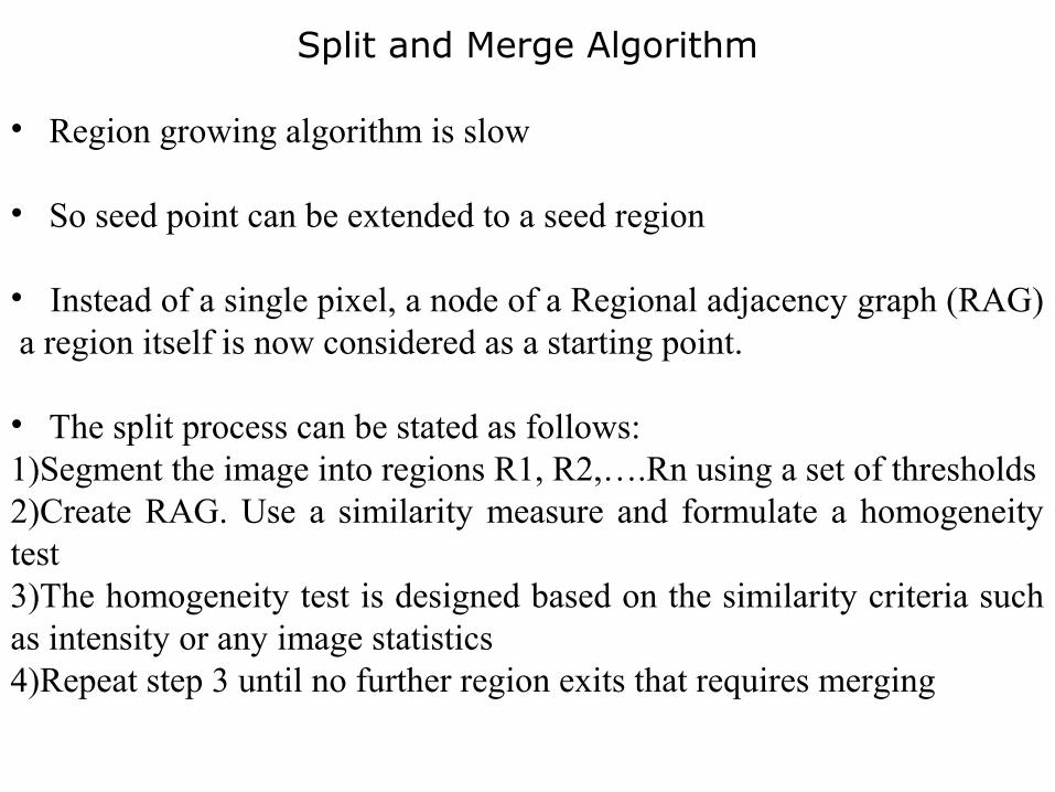
Split and Merge Algorithm
• Region growing algorithm is slow
• So seed point can be extended to a seed region
• Instead of a single pixel, a node of a Regional adjacency graph (RAG) a region itself is now considered as a starting point.
• The split process can be stated as follows:1)Segment the image into regions R1, R2,….Rn using a set of thresholds2)Create RAG. Use a similarity measure and formulate a homogeneity test3)The homogeneity test is designed based on the similarity criteria such as intensity or any image statistics4)Repeat step 3 until no further region exits that requires merging
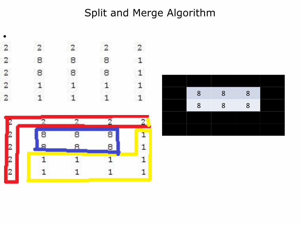
Split and Merge Algorithm
•
8 8 8
8 8 8
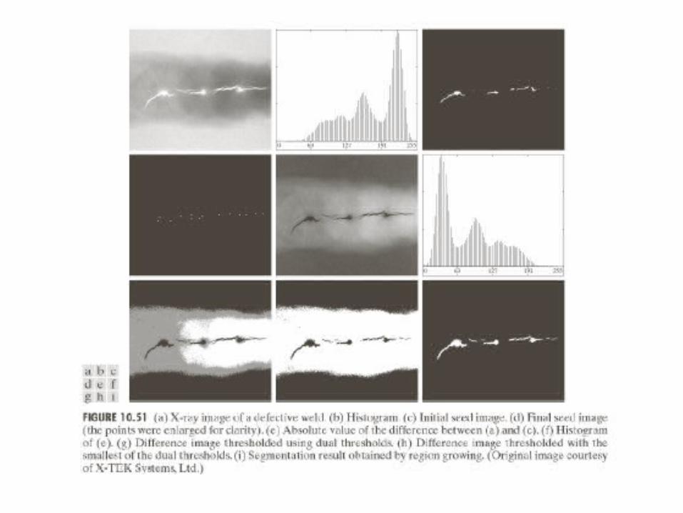
Region-Based SegmentationRegion Growing

Region-Based SegmentationRegion Growing
• Fig. 10.41 shows the histogram of Fig. 10.40 (a). It is difficult to segment the defects by thresholding methods. (Applying region growing methods are better in this case.)
Figure 10.41Figure 10.40(a)

Split and Merge using Quadtree
• Entire image is assumed as a single region. Then the homogeneity test is applied. If the conditions are not met, then the regions are split into four quadrants.
• This process is repeated for each quadrant until all the regions meet the required homogeneity criteria. If the regions are too small, then the division process is stopped.
•1) Split and continue the subdivision process until some stopping criteria is fulfilled. The stopping criteria often occur at a stage where no further splitting is possible.•2) Merge adjacent regions if the regions share any common criteria. Stop the process when no further merging is possible
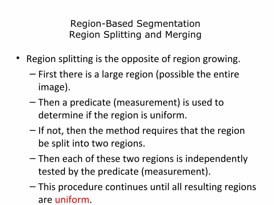
Region-Based SegmentationRegion Splitting and Merging
• Region splitting is the opposite of region growing.– First there is a large region (possible the entire
image).– Then a predicate (measurement) is used to
determine if the region is uniform. – If not, then the method requires that the region
be split into two regions. – Then each of these two regions is independently
tested by the predicate (measurement). – This procedure continues until all resulting regions
are uniform.
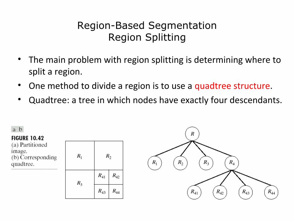
Region-Based SegmentationRegion Splitting
• The main problem with region splitting is determining where to split a region.
• One method to divide a region is to use a quadtree structure.• Quadtree: a tree in which nodes have exactly four descendants.
Region-Based SegmentationRegion Splitting and Merging
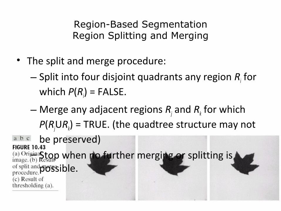
• The split and merge procedure:
– Split into four disjoint quadrants any region Ri for which P(Ri) = FALSE.
–Merge any adjacent regions Rj and Rk for which P(RjURk) = TRUE. (the quadtree structure may not be preserved)
– Stop when no further merging or splitting is possible.