chapter2: growth&decay

Intro to the TopicDiscrete Models

Growth and DecayLinear & Non-Linear Interaction Models

Introduction & Simple ModelsLogistic Growth Models

Chapter 2:

Growth & Decay

107 / 226




Introduction

In this chapter, model biological systems whose population isso large or where growth is so fine-grained that continuity canbe assumed.

These continuous models give rise to differential equations.

As a consequence, there is no natural time delay in the modelsand hence none of the over-compensation of differenceequations.

Extend the logistic growth equation model above & add aculling term.

Develop the ideas from this to a non-linear model for thechemostat.

108 / 226




Simple Models

For cell pop’n whose env’t doesn’t alter with time (i.e. ∞nutrients/ space), can assume that rate of increase of cells ∝number of cells.

Mathematically, can put this as:

dN

dt= rN (3.1)

for some constant of proportionality, r .

r measures average growth rate per unit time per individual(i.e. “2.4 children per person per life” number).

This equation (a.k.a.the law of organic growth) was namedafter Malthus4 a gloomy philosopher called who predicted (ca1798) that world pop’n would soon outgrow its resources.

4T.R. Malthus (1766-1834)109 / 226




Simple Models cont’d

In real life experiments there is always a finite starting value ofN at t = 0, N0. Can show that:

N(t) = N0ert (3.2)

i.e. (given ∞ space/ food) growth of cells is exponential.

Note that the value of the constant r can be -ive or +ive,corresponding to decay or growth respectively.

For a human population with α births per year & β deaths,obviously r = α− β & population viability depends on thisbeing +ive.

Can be shown from Eqn.(3.2) that doubling time for pop’ngiven by τ2 = ln 2/r so (if r is a percent) world’s populationdoubles itself every 70/r years.

110 / 226




Restricted Growth: the Verhulst or logistic model

Pop’ns do not grow in above manner; restrictions (due tofood, space, predation or any other factors) apply on allgrowth rates.

These put a limit on max sustainable pop’n size. This limit iscalled the carrying capacity of environment, K .

Instead of constant r given by Eqn.(3.1), have a timedependent growth rate 1

NdNdt.

Eqn.(3.1) implies a constant growth rate given by r .

111 / 226




Restricted Growth cont’d

In logistic growth model, growth rate is assumed to start at rwhen N = 0 & reach zero when N = K ,

Growth Rate ∝

(

1−N

K

)

i.e. the growth rate decreases linearly with increasingpopulation.

Mathematically logistic growth model is given by:

1

N

dN

dt= r

(

1−N

K

)

(3.3)

This differential equation involves parameters r , K :

r is relevant to initial growth phase of a pop’n (beforerestrictions have an effect)K imposes an upper limit on population growth.

112 / 226




Applications of the Model: r/K selection theory

In ecology, so-called r/K selection theory, relates to selectionof combinations of traits in a species that trade off btwquantity or quality of offspring.

r ,K refer to low- & high-density conditions, respectively.

Terminology came about from the work of the ecologistsMacArthur & Wilson based on their work on insulatedecosystems.

Species are often called either r-strategist or K-strategistdepending upon the selective processes shaping theirreproductive strategies.

Theory contends that adaptation to high or low densityenvironments involve different characteristics.

113 / 226




Applications of the Model: r/K selection theory cont’d

r-selection

In unstable/unpredictable environments, r-selection isdominant mechanism because ability to reproduce quickly iscrucial.

Adaptations that permit successful competition with otherorganisms are unnecessary, due to environmental volatility.

Characteristic traits of r-selection are thought to include:

short generation time,high fecundity & ability to disperse offspring widely,early maturity onset with small body size.

Examples range from bacteria, through insects (e.g.mosquitos) & weeds, to various mammals, especially smallrodents (e.g. rats).

114 / 226




Applications of the Model: r/K selection theory cont’d

K-selection

In stable/predictable environments, K-selection is dominantmechanism because ability to compete successfully for limitedresources is crucial.

Pop’n sizes of K-selected organisms typically very stable &approach max that the environment can bear.

Differ from r-selected populations, where population numbersare more volatile.Characteristic traits of K-selection are thought to include:

long life expectancy,mate choice,production of fewer offspring requiring extensive parental careuntil maturity & large body size.

Examples large organisms such as elephants, trees, humans &whales, but also some smaller organisms.

115 / 226




Further Applications of the Model

As well as above, Verhulst Model has been applied to other areas:

1 Spread of a Disease.

Initial no. of susceptible individuals to an infectious disease inpop’n is (a const) K.So y & (K − y) are no. of infectives & susceptibles after t.Chance encounters spread disease at a rate proportional to(product of) infectives & susceptibles.So model is y = ry(K − y)Spread of rumors is an example of an identical model to this.

116 / 226




Further Applications of the Model cont’d

2 Explosion/Extinction.

No. y(t) of crocs in a swamp satisfies y = ry wheregrowth-decay constant r ∝ (y −M) & M is a thresholdpopulation.The logistic model y = k(y −M)y gives extinction for initialpopulations smaller than M & a doomsday populationexplosion y(t)→∞ for y(0) > M .This model ignores harvesting/culling.

117 / 226





3 Logistic Growth with Culling.

No. y(t) of fish in a lake satisfies a logistic modely = (a− by)y − c , provided fish are harvested at a rate c > 0.This rate c can be either constant, variable (i.e. c = hy) orinvolve periodic harvesting & restocking c = hsin(ωt).These models are dealt with in more detail below

118 / 226





4 The Chemostat Model.

A chemostat (from Chemical environment is static) is abioreactor taking in fresh medium continuously, while cultureliquid is continuously removed to keep the culture volumeconstant.By changing rate with which medium is added to bioreactor,growth rate of microorganism can be easily controlled. Thismodel is examined below.

119 / 226





Solving the general form of logistic growth equationEqn.(3.3), (left as an exercise) to get:

N(t) =K

(

KN0− 1)

e−rt + 1(3.4)

for some inital population N0.

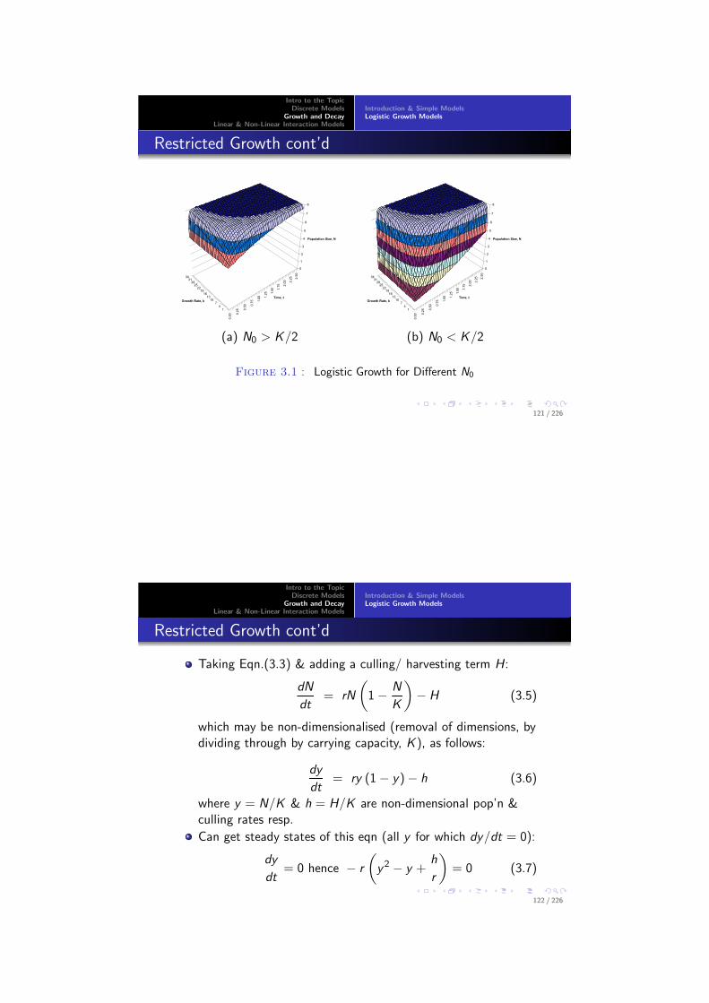
Can be seen from Figs 3.1(a) & (b) that logistic growth ofpop’n depends qualitatively on the initial population:

For N0 > K/2, second derivative N is always -tive,For N0 < K/2 there is a period of growth which is exp’l innature (N > 0) which then levels off (N = 0) before headingasymptotically to K (N < 0) as t →∞

120 / 226





0.00 0.25 0.50 0.75 1.00 1.25 1.50 1.75 2.00 2.25 2.50

1

4

7

10

13

16

1922

2528

3134

0

1

2

3

4

5

6

7

8

Population Size, N

Time, tGrowth Rate, k

(a) N0 > K/2

0.00 0.25 0.50 0.75 1.00 1.25 1.50 1.75 2.00 2.25 2.50

1

4

7

10

13

16

1922

2528

3134

0

1

2

3

4

5

6

7

8

Population Size, N

Time, tGrowth Rate, k

(b) N0 < K/2

Figure 3.1 : Logistic Growth for Different N0

121 / 226





Taking Eqn.(3.3) & adding a culling/ harvesting term H:

dN

dt= rN

(

1−N

K

)

− H (3.5)

which may be non-dimensionalised (removal of dimensions, bydividing through by carrying capacity, K ), as follows:

dy

dt= ry (1− y)− h (3.6)

where y = N/K & h = H/K are non-dimensional pop’n &culling rates resp.

Can get steady states of this eqn (all y for which dy/dt = 0):

dy

dt= 0 hence − r

(

y2 − y +h

r

)

= 0 (3.7)

122 / 226





Provided they meet the harvesting condition 4h < r , bothroots of Eqn 3.7:

y = p± =1

2

(

1±

√

1−4h

r

)

(3.8)

are steady states since both have the property y = N/K < 1.

Note: condition 4h < r gives us population harvestingcapacity (i.e. how much may be harvested).

In order to find stable states of Eqn.(3.6), it is necessary tograph the derivative of y against y itself.

This allows us to examine the behaviour of the derivative forvarious (especially initial) values of y .

123 / 226





Examining the graph (Fig. 3.2), see that points p− and p+from Eqn.(3.8) demarcate areas of stability.

For y(0) < p−, pop’n will never grow, as y < 0 for all t andthus extinction will occur.

For y(0) > p−, y > 0 & pop’n will eventually settle down to asteady state y = p+ (this follows from working out a solutionto Eqn.(3.6) and examining behaviour of y(t) as t →∞).

Can be seen from Fig 3.2, that the time of optimum culling isthe point where y is maximal. Before this pop’n is notgrowing at an optimal rate. After this growth rate isdecreasing to the steady state.

124 / 226





dydt

y = p−

y = p+

y(t)

Figure 3.2 : y V y for Logistic Growth with Culling

125 / 226




Aside: Equilibrium & Stability

A constant solution of a differential equation is called anequilibrium solution or steady state.

Locating/ classifying steady states helps determine family ofall solutions of DE equation.

Soln to a DE of form N(t) = constant, because dN/dt = 0 iscalled an equilibrium point.

126 / 226




Aside: Equilibrium & Stability cont’d

Classify steady states according to behavior of other solutionsthat start nearby:

Steady states N = c is called stable if any solution N(t) thatstarts near N = c stays near it.Equilibrium N = c is called asymptotically stable if anysolution N(t) that starts near N = c actually converges to it,that is limt→∞ = c .If an equilibrium state is not stable, it is called unstable. Thismeans there is at least one solution that starts near equilibrium& runs away from it.Example of this is first state N = 0 of the Logistic Growthmodel with no culling (similar to Fig. 3.2, only shifted to theleft to have roots at N = 0 and N = K ) Eqn.(3.3), this is anunstable state. This is because, if N = +ǫ (for small ǫ), thepopulation will increase; if N = −ǫ, the population willdecrease further.

127 / 226




The Chemostat

Logistic Growth model can be used for Chemostat, (used tostudy growth of µorganisms under various lab conditions).

For the growth models so far, since the nutrients are notrenewed, exp’l growth is limited to a few generations.

Bacterial cultures can be maintained in a state of exp’l growthfor long time using a system of continuous culture, designed torelieve the conditions that stop exp’l growth in batch cultures.

Such continuous culture, in the chemostat, is a situation thatreflects bacterial growth in natural environments.

In chemostat, growth chamber is connected to a reservoir ofsterile medium.

Once growth is initiated, fresh medium is continuouslysupplied from reservoir.

128 / 226




The Chemostat cont’d

Fluid volume in growth chamber is maintained at constantlevel by an overflow drain.

Fresh medium enters growth chamber at a rate that limitsbacterial growth.

Bacteria grow at same rate that overflow removes bacterialcells & spent medium.

Fresh medium addition rate determines growth rate cos freshmedium contains limiting amount of essential nutrient.

Thus, chemostat relieves lack of nutrients, toxic substanceaccumulation, & accumulation of excess cells in culture, whichinitiate growth cycle’s stationary phase.

Bacterial culture can be grown and maintained at relativelyconstant conditions, depending on nutrient flow rate.

129 / 226





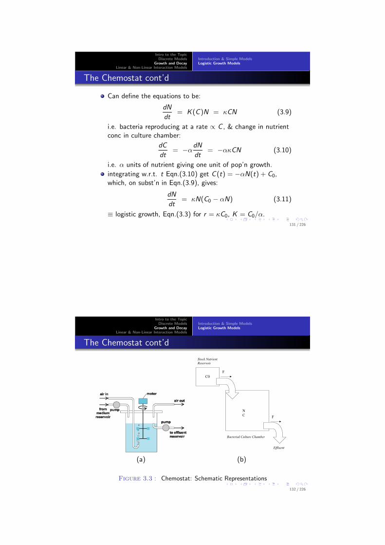
For Chemostat, model is more complicated than for purelogistic growth with a limited volume of nutrient Eqn.(3.3); ascan be seen in Fig. 3.3(b), there is an inflow rate into thecentral culture chamber and also an outflow rate from thechamber.

These latter two terms are both F to conserve mass inchamber.

To start, will derive logistic growth model again, formicroorganism pop’n N, taking into account nutrient concC (t).

130 / 226





Can define the equations to be:

dN

dt= K (C )N = κCN (3.9)

i.e. bacteria reproducing at a rate ∝ C , & change in nutrientconc in culture chamber:

dC

dt= −α

dN

dt= −ακCN (3.10)

i.e. α units of nutrient giving one unit of pop’n growth.

integrating w.r.t. t Eqn.(3.10) get C (t) = −αN(t) + C0,which, on subst’n in Eqn.(3.9), gives:

dN

dt= κN(C0 − αN) (3.11)

≡ logistic growth, Eqn.(3.3) for r = κC0, K = C0/α.

131 / 226





(a)

&�

1

&

)

)

(IIOXHQW

%DFWHULDO�&XOWXUH�&KDPEHU

6WRFN�1XWULHQW

5HVHUYRLU

(b)

Figure 3.3 : Chemostat: Schematic Representations

132 / 226




Chemostat Parameters

Quantity Symbol units

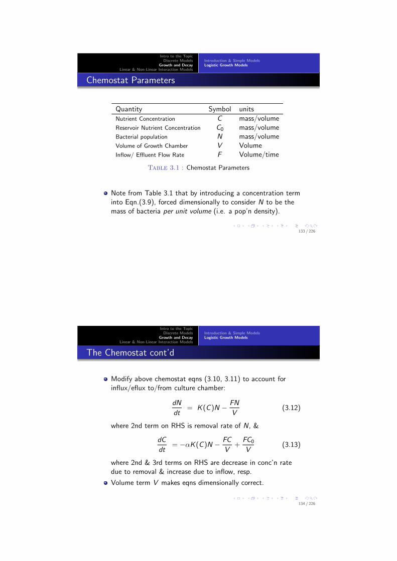
Nutrient Concentration C mass/volumeReservoir Nutrient Concentration C0 mass/volumeBacterial population N mass/volumeVolume of Growth Chamber V VolumeInflow/ Effluent Flow Rate F Volume/time

Table 3.1 : Chemostat Parameters

Note from Table 3.1 that by introducing a concentration terminto Eqn.(3.9), forced dimensionally to consider N to be themass of bacteria per unit volume (i.e. a pop’n density).

133 / 226





Modify above chemostat eqns (3.10, 3.11) to account forinflux/eflux to/from culture chamber:

dN

dt= K (C )N −

FN

V(3.12)

where 2nd term on RHS is removal rate of N, &

dC

dt= −αK (C )N −

FC

V+

FC0

V(3.13)

where 2nd & 3rd terms on RHS are decrease in conc’n ratedue to removal & increase due to inflow, resp.

Volume term V makes eqns dimensionally correct.

134 / 226

chapter2: growth&decay

Documents