chapter32 corporatevaluation

Chapter 32

CORPORATE VALUATION

Centre for Financial Management , Bangalore

OUTLINE• Importance of valuation

• Goal of valuation

• Adjusted book value approach

• Analysing historical performance

• Discounted cash flow approach

• Estimating the cost of capital

• Forecasting performance

• Determining the continuing value

• Calculating the firm value and interpreting the results

• DCF valuation: 2-stage and 3-stage growth models

• Free cash flow to equity valuation

• Guidelines for equity valuation Centre for Financial Management , Bangalore

IMPORTANTCE OF VALUATION

In the wake of economic liberalisation, companies are

relying more on the capital market, acquisitions and

restructuring are becoming commonplace, strategic

alliances are gaining popularity, employee stock option

plans are proliferating, and regulatory bodies are

struggling with tariff determination. In these exercises a

crucial issue is: How should the value of a company or a

division thereof be appraised?


GOAL OF VALUATION

The goal of such an appraisal is essentially to estimate a fair market value of a company. So, at the outset, we must clarify what is meant by “fair market value” and what is meant by “a company”. The most widely accepted definition of fair market value was laid down by the Internal Revenue Service of the US. It defined fair market value as "the price at which the property would change hands between a willing buyer and a willing seller when the former is not under any compulsion to buy and the latter is not under any compulsion to sell, both parties having reasonable knowledge of relevant facts.” When the asset being appraised is “a company”, the property the buyer and the seller are trading consists of the claims of all the investors of the company. This includes outstanding equity shares, preference shares, debentures, and loans.


APPROACHES TO VALUATION

There are four broad approaches to appraising the value of a company:

• Adjusted book value approach

• Stock and debt approach

• Direct comparison approach

• Discounted cash flow approach


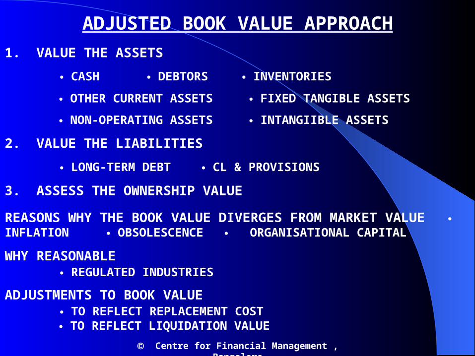
ADJUSTED BOOK VALUE APPROACH1. VALUE THE ASSETS

CASH DEBTORS INVENTORIES

OTHER CURRENT ASSETS FIXED TANGIBLE ASSETS

NON-OPERATING ASSETS INTANGIIBLE ASSETS

2. VALUE THE LIABILITIES

LONG-TERM DEBT CL & PROVISIONS

3. ASSESS THE OWNERSHIP VALUE

REASONS WHY THE BOOK VALUE DIVERGES FROM MARKET VALUE INFLATION OBSOLESCENCE ORGANISATIONAL CAPITAL

WHY REASONABLE REGULATED INDUSTRIES

ADJUSTMENTS TO BOOK VALUE TO REFLECT REPLACEMENT COST TO REFLECT LIQUIDATION VALUE


BALANCE SHEET OF HORIZON LIMITED AS ON MARCH 31, 2001 ( Rs in million)

CAPITAL AND LIABILITIES ASSETS

SHARE CAP 15.0 FIXED ASSETS 33.0

RES. AND SURP 11.2 INVESTMENTS 1.5

LOAN FUNDS 21.2 CURRENT ASSETS 23.4

CURR LIAB 10.5

57.9 57.9

BALANCE SHEET VALUATIONINVESTOR CLAIMS APPROACH ASSET-LIABILITIES APPROCH

SHARE CAP 15.0 TOTAL ASSETS 57.9

RES. AND SURP 11.2 LESS : CURRENT LIAB 10.5

LOAN FUNDS 21.247.4 47.4


STOCK AND DEBT APPROACH

• PUBLICLY TRADED

• WHAT PRICE ?

AVERAGING ?

EMH . . .

• TWO IMPLICATIONS

• S & D . . MOST RELIABLE ESTIMATE OF VALUE

• SECURITIES . . VALUED . . LIEN DATE Centre for Financial Management , Bangalore

DIRECT COMPARISON APPROACHCommon sense and economic logic tell us that similar assets should sell at similar prices. Based on this principle, one can value an asset by looking at the price at which a comparable asset has changed hands between a reasonably informed buyer and a reasonably informed seller. This approach, referred to as the direct comparison approach, is commonly applied in real estate. Essentially, the direct comparison approach is reflected in a simple formula:

Vc

VT = xT . (32.1) xc

where VT = appraised value of the target firm (or asset)

xT = observed variable for the target firm that supposedly drives value

Vc = observed value of the comparable firm xc = observed variable for the comparable company Centre for Financial Management , Bangalore

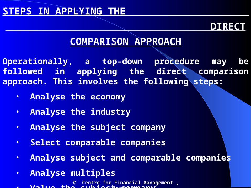
STEPS IN APPLYING THE DIRECT COMPARISON APPROACH

Operationally, a top-down procedure may be followed in applying the direct comparison approach. This involves the following steps:

• Analyse the economy

• Analyse the industry

• Analyse the subject company

• Select comparable companies

• Analyse subject and comparable companies

• Analyse multiples

• Value the subject company


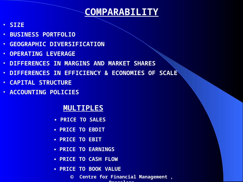
COMPARABILITY• SIZE• BUSINESS PORTFOLIO• GEOGRAPHIC DIVERSIFICATION• OPERATING LEVERAGE• DIFFERENCES IN MARGINS AND MARKET SHARES• DIFFERENCES IN EFFICIENCY & ECONOMIES OF SCALE• CAPITAL STRUCTURE• ACCOUNTING POLICIES

MULTIPLES PRICE TO SALES

PRICE TO EBDIT

PRICE TO EBIT

PRICE TO EARNINGS

PRICE TO CASH FLOW

PRICE TO BOOK VALUE Centre for Financial Management , Bangalore

ILLUSTRATIONThe following financial information is available for company D, a pharmaceutical company,

Profit before depreciation interest and taxes (PBDIT) Rs.18 million Book value of assets Rs.90 million Sales Rs.125 million

Based on an evaluation of several pharmaceutical companies, companies A, B, and C have been found to be comparable to company D. The financial information for these companies is given below.

A B C

PBDIT* 12 15 20 Book value of assets* 75 80 100 Sales* 80 100 160 Market value* (MV) 150 240 360 MV/PBDIT 12.5 16.0 18.0 MV/Book value 2.0 3.0 3.6 MV/Sales 1.9 2.4 2.3

*In million rupees


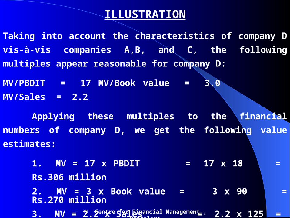
ILLUSTRATION.

Taking into account the characteristics of company D vis-à-vis companies A,B, and C, the following multiples appear reasonable for company D:

MV/PBDIT = 17 MV/Book value = 3.0 MV/Sales = 2.2

Applying these multiples to the financial numbers of company D, we get the following value estimates:

1. MV = 17 x PBDIT = 17 x 18 = Rs.306 million2. MV = 3 x Book value = 3 x 90 = Rs.270 million3. MV = 2.2 x Sales = 2.2 x 125 = Rs.275 million

A simple arithmetic average of the three value estimates is :

(306 + 270 + 275) / 3 = Rs.283.7 million


PROS AND CONS OF MARKET APPROACH

• MULTIPLES ARE SIMPLE AND EASY TO RELATE TO

• MULTIPLES ARE AMENABLE TO MISUSE AND MANIPULATE

• CHOICE OF COMPARABLE COMPANIES DISGUISES SUBJECTIVE BIAS –IN DCF APPROACH ASSUMPTIONS HAVE TO BE MORE EXPLICIT.

• BUILDS IN ERRORS OF MARKET VALUATION

• DCF VAL’N . . BASED . . ON FIRM SPECIFIC GROWTH RATES & CASH SPECIFIC GROWTH RATES & CASH FLOWS


DISCOUNTED CASH FLOW APPROACH

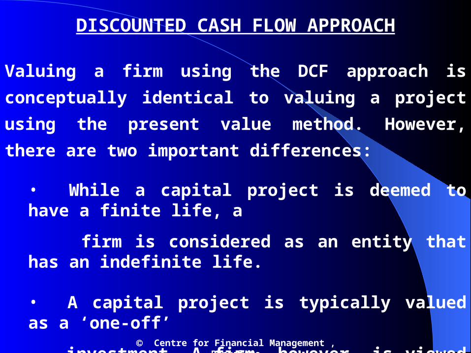
Valuing a firm using the DCF approach is conceptually identical to valuing a project using the present value method. However, there are two important differences:

• While a capital project is deemed to have a finite life, a

firm is considered as an entity that has an indefinite life.

• A capital project is typically valued as a ‘one-off’

investment. A firm, however, is viewed as a growing

entity requiring continuing investments



To sum up, valuing a firm using the discounted cash flow approach calls for forecasting cash flows over an indefinite period of time for an entity that is expected to grow. This is indeed a daunting proposition. To tackle this task, in practice, the value of the firm is separated into two time periods:

Value of the firm = Present value of cash flow + Present value of cash flow during an explicit forecast after the explicit forecast period period

During the explicit forecast period – which is often a period of 5 to 15 years – the firm is expected to evolve rather rapidly and hence a great deal of effort is expended to forecast its cash flow on an annual basis. At the end of the explicit forecast period, the firm is expected to reach a “steady state” and hence a simplified procedure is used to estimate its continuing value



Thus, the discounted cash flow approach to valuing a firminvolves the following steps:

1. Analysing historical performance

2. Estimating the cost capital

3. Forecasting performance

4. Determining the continuing value

5. Calculating the firm value and interpreting the results.


ANALYSING HISTORICAL PERFORMANCE

Inter alia, historical performance analysis should focus on:

• Extracting valuation related metrics from accounting

statements.

• Calculating the free cash flow and the cash flow available

to investors

• Getting a perspective on the drivers of free cash flow

• Developing the ROIC tree Centre for Financial Management , Bangalore

Financial Statements of Matrix Limited for the Preceding

Three Years (Years 1-3)


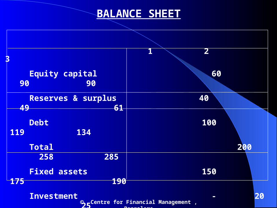
1 2 3

Equity capital 60 90 90

Reserves & surplus 40 49 61

Debt 100 119 134

Total 200 258 285

Fixed assets 150 175 190

Investment - 20 25

Net current assets 50 63 70

Total 200 258 285

BALANCE SHEET


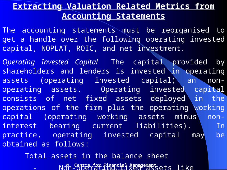
Extracting Valuation Related Metrics from Accounting Statements

The accounting statements must be reorganised to get a handle over the following operating invested capital, NOPLAT, ROIC, and net investment.

Operating Invested Capital The capital provided by shareholders and lenders is invested in operating assets (operating invested capital) an non-operating assets. Operating invested capital consists of net fixed assets deployed in the operations of the firm plus the operating working capital (operating working assets minus non-interest bearing current liabilities). In practice, operating invested capital may be obtained as follows:

Total assets in the balance sheet

- Non-operating fixed assets like surplus land

- Excess cash and marketable securities1 1 This represents cash and marketable securities in excess of the operational needs of the firm.


Extracting Valuation Related Metrics from Accounting Statements

If we assume that the investment figures of 20 and 25 in the balance sheet of Matrix Limited at the end of years 2 and 3 represent excess cash and marketable securities, the operating invested capital at the end of years 1, 2, and 3 for Matrix Limited is:

1 2 3

Operating invested 200 238 260

capital


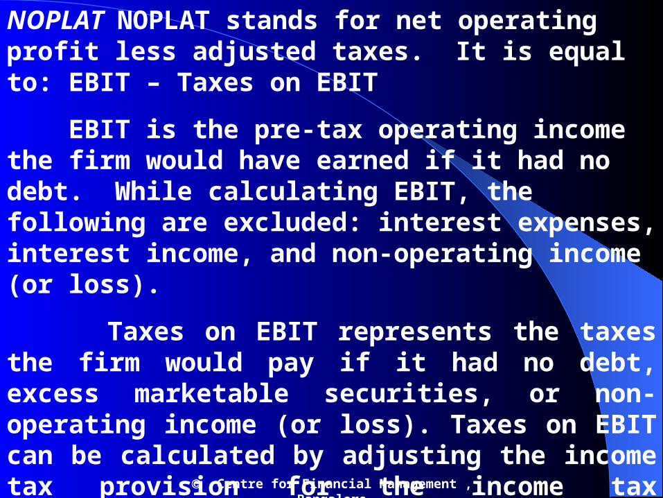
NOPLAT NOPLAT stands for net operating profit less adjusted taxes. It is equal to: EBIT – Taxes on EBIT

EBIT is the pre-tax operating income the firm would have earned if it had no debt. While calculating EBIT, the following are excluded: interest expenses, interest income, and non-operating income (or loss).

Taxes on EBIT represents the taxes the firm would pay if it had no debt, excess marketable securities, or non-operating income (or loss). Taxes on EBIT can be calculated by adjusting the income tax provision for the income tax attributable to interest expense, interest and dividend income from excess marketable securities and, non-operating income (or loss).



The calculation of NOPLAT for Matrix Limited is shown below

Return on Invested Capital

Return on invested capital, ROIC, is defined as follows: NOPLAT

ROIC = Invested capital

Invested capital is usually measured at the beginning of the year or as the average at the beginning and end of the year. While calculating ROIC, define the numerator and denominator consistently. If an asset is included in invested capital, income related to it should be included in NOPLAT to achieve consistency. The ROIC for Matrix Limited is calculated below: Year 2 Year 3NOPLAT 30 27Invested capital at the 200 238beginning of the yearROIC 30/200 = 15% 27/238 = 11.3%

ROIC focuses on the true operating performance of the firm. It is a better measured compared to return on equity and return on assets. Return on equity reflects operating performance as well as financial structure and return on assets is internally inconsistent (numerator and denominator are not consistent). Centre for Financial Management , Bangalore

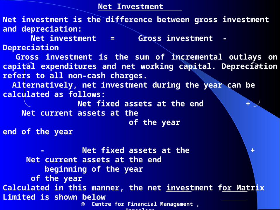
Net Investment

Net investment is the difference between gross investment and depreciation:Net investment = Gross investment - Depreciation

Gross investment is the sum of incremental outlays on capital expenditures and net working capital. Depreciation refers to all non-cash charges. Alternatively, net investment during the year can be calculated as follows: Net fixed assets at the end + Net current assets at the of the year end of the year

- Net fixed assets at the + Net current assets at the end beginning of the year of the year

Calculated in this manner, the net investment for Matrix Limited is shown below Year 2 Year 3 Net fixed assets at the end 175 190 of the year+ Net current assets at the 63 70 at the end of the year- Net fixed assets at the beginning 150 175 of the year- Net current assets at the 50 63 beginning of the year 38 22


Calculating the Free Cash Flow

The free cash flow (FCF) is the post-tax cash flow generated from the operations of the firm after providing for investments in fixed investment and net working capital required for the operations of the firm. FCF can be expressed as:

FCF = NOPLAT - Net investmentFCF = (NOPLAT + Depreciation) - (Net investment + Depreciation)FCF = Gross cash flow - Gross investment

Exhibit shows the FCF calculation for Matrix LimitedMatrix Limited Free Cash Flow Year 1 Year 2 Year 3

NOPLAT 25.2 30.0 27.0Depreciation 12 15 18Gross cash flow 37.2 45 45(Increase)/decrease in 13 7 working capital Capital expenditure 40 33Gross investment 53 40Free cash flow (8) 5

CASH FLOW AVAILABLE TO INVESTORS

The cash flow available to investors (shareholders and lenders) is equal to free cash flow plus non-operating cash flow .We have discussed what free cash flow is. What is non-operating cash flow? Non-operating cash flow arises from non-operating items like sale of assets, restructuring, and settlement of disputes. Such items must, of course, be adjusted for taxes.


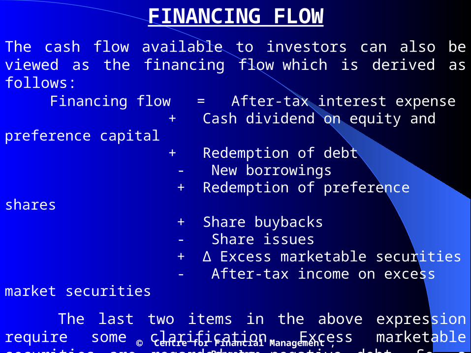
FINANCING FLOWThe cash flow available to investors can also be viewed as the financing flow which is derived as follows: Financing flow = After-tax interest expense + Cash dividend on equity and preference capital

+ Redemption of debt - New borrowings + Redemption of preference shares + Share buybacks - Share issues + Δ Excess marketable securities - After-tax income on excess market securities

The last two items in the above expression require some clarification. Excess marketable securities are regarded as negative debt. So, a change in excess marketable securities is treated a financing flow. For the same reason, the post-tax income on excess marketable securities is regarded as a financing flow.


MATRIX LIMITED – CASH FLOW AVAILABLE TO

INVESTORS


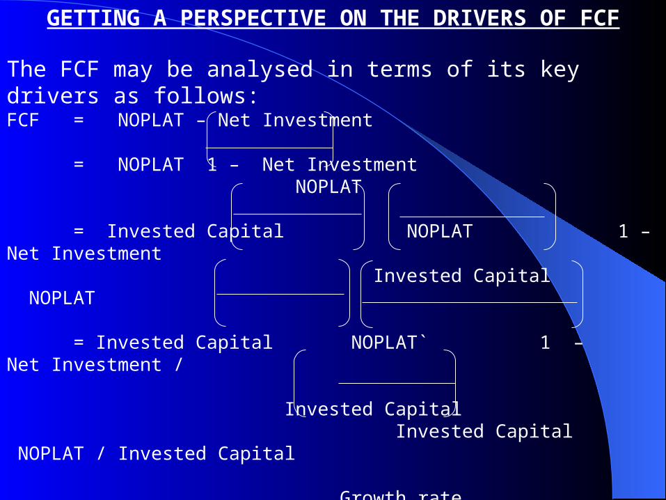
GETTING A PERSPECTIVE ON THE DRIVERS OF FCF

The FCF may be analysed in terms of its key drivers as follows:FCF = NOPLAT – Net Investment

= NOPLAT 1 – Net Investment NOPLAT

= Invested Capital NOPLAT 1 – Net Investment Invested Capital NOPLAT

= Invested Capital NOPLAT` 1 – Net Investment / Invested Capital Invested Capital NOPLAT / Invested Capital

Growth rate = Invested capital x ROIC x 1 -

ROIC

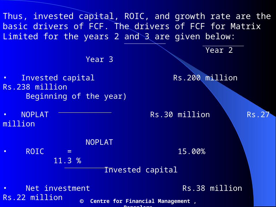
Thus, invested capital, ROIC, and growth rate are the basic drivers of FCF. The drivers of FCF for Matrix Limited for the years 2 and 3 are given below:

Year 2 Year 3

• Invested capital Rs.200 million Rs.238 million Beginning of the year)

• NOPLAT Rs.30 million Rs.27 million

NOPLAT• ROIC = 15.00% 11.3 %

Invested capital

• Net investment Rs.38 million Rs.22 million

Net investment• Growth rate = 19.00% 9.2%

Invested capital• FCF -Rs.8 million Rs.5 million


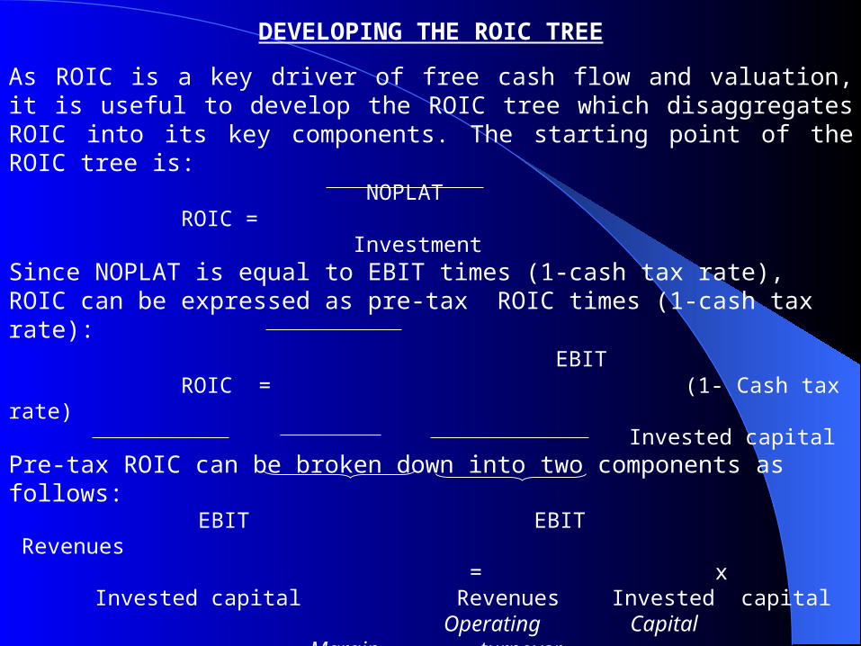
DEVELOPING THE ROIC TREE

As ROIC is a key driver of free cash flow and valuation, it is useful to develop the ROIC tree which disaggregates ROIC into its key components. The starting point of the ROIC tree is: NOPLAT

ROIC = Investment Since NOPLAT is equal to EBIT times (1-cash tax rate), ROIC can be expressed as pre-tax ROIC times (1-cash tax rate): EBIT

ROIC = (1- Cash tax rate) Invested capital Pre-tax ROIC can be broken down into two components as follows:

EBIT EBIT Revenues = x Invested capital Revenues Invested capital Operating Capital

Margin turnover The first term, viz, operating margin measures how effectively the firm converts revenues into profits and the second term, viz, capital turnover reflects how effectively the company employs its invested capital. Each of these two components can be further disaggregated. Exhibit 32.6 shows the ROIC tree for Matrix Limited.

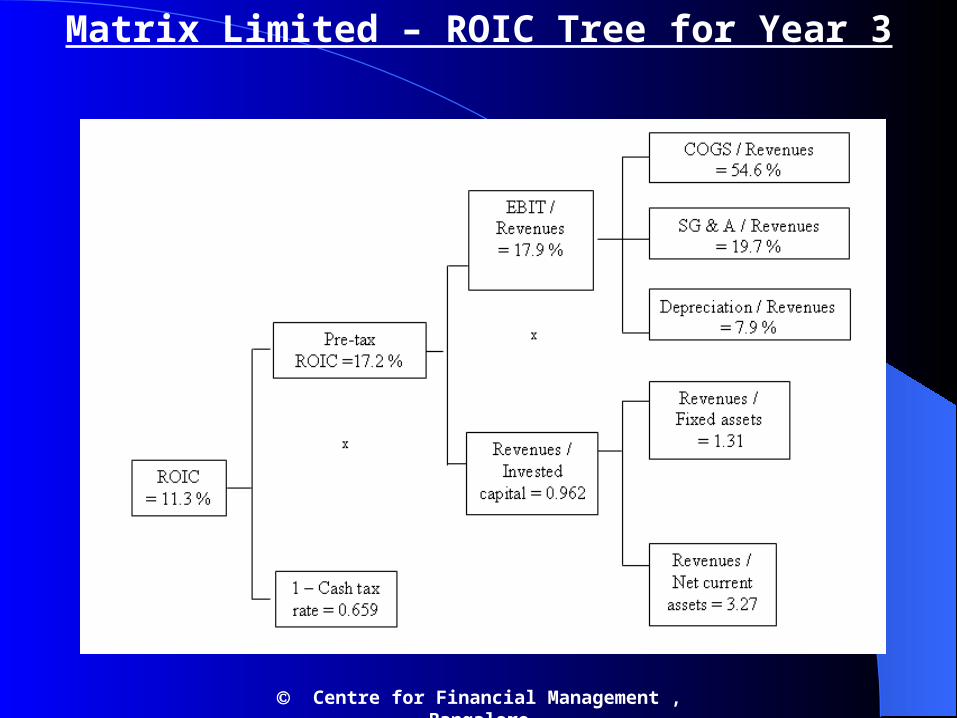
Matrix Limited – ROIC Tree for Year 3


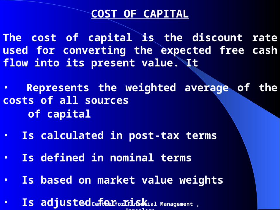
COST OF CAPITAL

The cost of capital is the discount rate used for converting the expected free cash flow into its present value. It

• Represents the weighted average of the costs of all sources of capital

• Is calculated in post-tax terms

• Is defined in nominal terms

• Is based on market value weights

• Is adjusted for risk


FORMULAThe formula that may be employed for estimating the weighted average cost of capital is:

WACC = rE (S/V) + rP (P/V) + rD(1-T) (B/V) (32.1)

where WACC = weighted average cost of capital

rE = cost of equity capital S = market value of equity V = market value of the firm

rp = cost of preference capital P = market value of preference capital

rD = pre-tax cost of debt T = marginal rate of tax applicable B = market value of interest-bearing debt


MATRIX’S WEIGHTED AVERAGE COST OF CAPITAL

Matrix Limited has a target capital structure in which debt and equity have weights (in market value terms) of 2 and 3. The component costs of debt and equity are 12.67 percent and 18.27 percent. The marginal tax rate for Matrix is 40 percent. Given this information the, weighted average cost of capital is calculated as follows:

3 2

WACC = x 18.27 + x 12.67% (1 - .4)

5 5

= 10.96 + 3.04 = 14 percent


FORECASTING PERFORMANCE

After analysing historical performance and estimating the cost of capital, we move on to developing a financial forecast. This involves the following steps.

1. Selecting the explicit forecast period.

2. Developing a strategic perspective on the future performance of the company.

3. Converting the strategic perspective into financial forecasts.

4. Checking for consistency and alignment.


SELECTING THE EXPLICIT FORECAST PERIOD

The general guideline is that the explicit forecast period should be such that the business reaches a steady state at the end of this period. This condition has to be satisfied because typically the continuing value formula is based on the following assumptions: (i) The firm earns a fixed profit margin, achieves a constant asset turnover, and hence earns a constant rate of return on the invested capital. (ii) The re-investment rate (the proportion of gross cash flow invested annually) and the growth rate remain constant.


DEVELOPING A STRATEGIC PERSPECTIVE

The strategic perspective reflects a credible story about the company’s future performance. One such story about a telecom software provider is given below for illustrative purposes:

“ The global telecom market is recovering. The company is well-positioned in those segments of the telecom market which are growing rapidly. The company has restructured its licensing arrangements with its customers and this is expected to augment its overall income from licensing. The combination of these factors is expected to generate a robust growth in revenues and improve the net profit margin over the next five years.”


CONVERTING THE STRATEGIC PERSPECTIVE INTO A FINANCIAL FORECAST

Once you have crafted a story about the company’s future

performance, you have to develop a forecast of free cash flow.

Sometimes the free cash flow forecast is developed directly

without going through the profit and loss account and the

balance sheet. However, it is advisable to base the free cash

flow forecast on an integrated profit and loss account and

balance sheet forecast. This provides a proper perspective on

how the various elements fit together. Centre for Financial Management , Bangalore

CONVERTING THE STRATEGIC PERSPECTIVE INTO A FINANCIAL FORECAST


For non-financial companies, the most common method for forecasting the profit and loss account and the balance sheet is as follows:

1. Develop the revenue forecast on the basis of volume growth and price changes.

2. Use the revenue forecast to estimate operating costs, working capital, and fixed assets.

3. Forecast non-operating items such as investments, non-operating income, interest expense, and interest income.

4. Project net worth. Net worth at the end of year n is equal to net worth at the end of year n-1, plus the amount ploughed back from the earnings of year n, plus new share issues during year n, minus share repurchases during year n.

5. Use the cash and / or debt account as the balancing account.

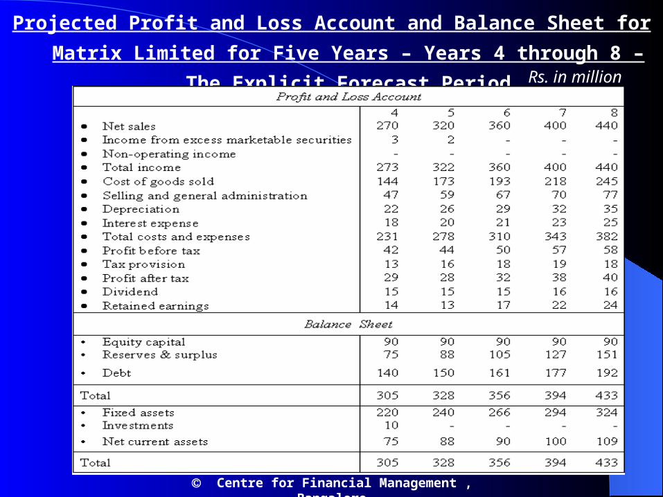
Projected Profit and Loss Account and Balance Sheet for Matrix Limited for Five Years – Years 4 through 8 – The Explicit Forecast Period


Rs. in million

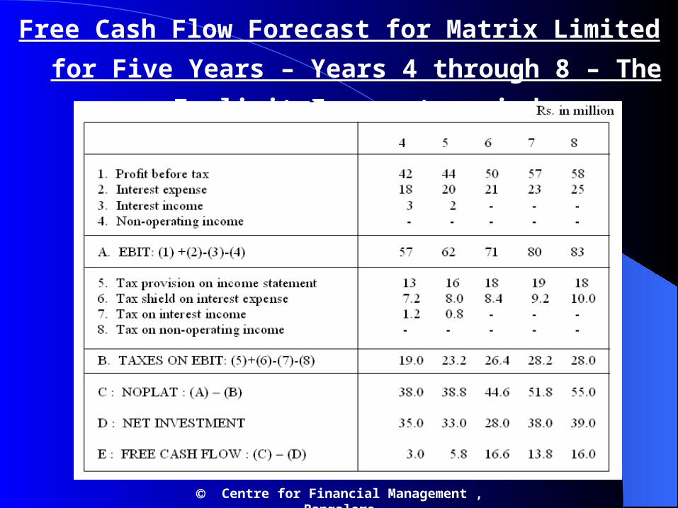
Free Cash Flow Forecast for Matrix Limited for Five Years – Years 4 through 8 – The Explicit Forecast period


CHECKING FOR CONSISTENCY AND ALIGNMENT

The final step in the forecasting exercise is to evaluate the forecast for consistency and alignment by asking the following questions.

• Is the projected revenue growth consistent with industry growth?• Is the ROIC justified by the industry’s competitive structure?• What will be the impact of technological changes on risk and returns?• Is the company capable of managing the proposed investments?• Will the company be in a position to raise capital for its expansion needs?

Because ROIC and growth are the key drivers of value, let us look at how companies have performed on these parameters. Empirical evidence suggest that:

• Industry average ROICs and growth rates are related to economic fundamentals. For example, the pharmaceutical industry, thanks to patent protection, enjoys a higher ROIC whereas the automobile industry earns a lower ROIC because of its capital intensity.

• It is very difficult for a company to out perform its peers for an extended period of time because competition often catches up, sooner or later.


DETERMINING THE CONTINUING VALUE

As discussed earlier, a company’s value is the sum of two terms:

Present value of cash flow during + Present value of cash flow the explicit forecast period after the explicit forecast period

The second term represents the continuing value or the terminal value. It is the value of the free cash flow beyond the explicit forecast period. Typically, the terminal value is the dominant component in a company’s value. Hence, it should be estimated carefully and realistically.

There are two steps in estimating the continuing value:

• Choose an appropriate method• Calculate the continuing value


CHOOSING AN APPROPRIATE METHODA variety of methods are available for estimating the continuing value. They may be classified into two broad categories as follows:

Cash Flow Methods Non-cash Flow Methods• Growing free cash flow perpetuity method

• Replacement cost method

• Value driver method • Price-PBIT ratio method

• Market-to-book ratio method


GROWING FREE CASH FLOW PERPETUITY METHOD

This method assumes that the free cash flow would grow at a constant rate for ever, after the explicit forecast period, T. Hence, the continuing value of such a stream can be established by applying the constant growth valuation model:

FCFT+1

CVT = (32.2)WACC – g

where CVT is the continuing value at the end of year T, FCFT+1 is the expected free cash flow for the first year after the explicit forecast period, WACC is the weighted average cost of capital, and g is the expected growth rate of free cash flow forever.


VALUE DRIVER METHOD

This method too uses the growing free cash flow perpetuity formula but expresses it in terms of value drivers as follows:

NOPLATT+1 (1 – g / r)CVT = (32.3)

WACC – gwhere CVT is the continuing value at the end of year T, NOPLATT+1 is the expected net operating profits less adjusted tax for the first year after the explicit forecast period, WACC is the weighted average cost of capital, g is the constant growth rate of NOPLAT after the explicit forecast period, and r is the expected rate of return on net new investment. The formulae given in Eqns (32.2) and (32.3) produce the same result as they have the same denominator, and the numerator in Eqn (32.3) is a different way of expressing the free cash flow (the numerator of Eqn (32.2).


REPLACEMENT COST METHOD

According to this method, the continuing value is equated with the expected replacement cost of the fixed assets of the company. This method suffers from two major limitations: (i) Only tangible assets can be replaced. The “organisational capital” (reputation of the company; brand image; relationships with suppliers, distributors, and customers; technical know-how; and so on) can only be valued with reference to the cash flows the firm generates in future, as it cannot be separated from the business as a going entity. Clearly, the replacement cost of tangible assets often grossly understates the value of the firm. (ii) It may simply be uneconomical for a firm to replace some of its assets. In such cases, their replacement cost exceeds their value to the business as a going concern.


PRICE-TO-PBIT RATIO METHOD

A commonly used method for estimating the continuing value is the price-to-PBIT ratio method. The expected PBIT in the first year after the explicit forecast period is multiplied by a ‘suitable’ price-to-PBIT ratio. The principal attraction of this method is that the price-to-PBIT ratio is a commonly cited statistic and most executives and analysts feel comfortable with it. Notwithstanding the practical appeal of the price-to-PBIT ratio method, it suffers from serious limitations: (i) It assumes that PBIT drives prices. PBIT, however, is not a reliable bottom line for purposes of economic evaluation. (ii) There is an inherent inconsistency in combining cash flows during the explicit forecast period with PBIT (an accounting number) for the post-forecast period. (iii) There is a practical problem as no reliable method is available for forecasting the price-to-PBIT ratio.


MARKET-TO-BOOK RATIO METHOD

According to this method, the continuing value of the company at the end of the explicit forecast period is assumed to be some multiple of its book value. The approach is conceptually analogous to the price-PBIT ratio, and, hence, suffers from the same problems. Further, the distortion in book value on account of inflation and arbitrary accounting policies may be high. Overall, it appears that the cash flow methods are superior to the non-cash flow methods.


CALCULATING THE CONTINUING VALUE

The growing free cash flow perpetuity method is commonly used for estimating the continuing value. The key inputs required for this method are the weighted average cost of capital (WACC) and the constant growth rate (g). The WACC has been estimated at 14 percent. If we assume that g is 10 percent, the continuing value of Matrix Limited at the end of year 8 can be calculated as follows.

FCF9 FCF8 (1 + g)Continuing value8 = = WACC - g WACC - g

16 (1.10) = = Rs.440 million

0.14 - 0.10


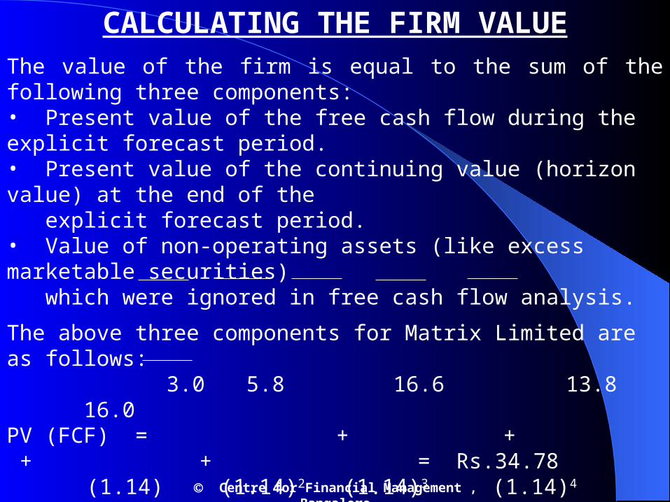
CALCULATING THE FIRM VALUEThe value of the firm is equal to the sum of the following three components:• Present value of the free cash flow during the explicit forecast period.• Present value of the continuing value (horizon value) at the end of the explicit forecast period.• Value of non-operating assets (like excess marketable securities) which were ignored in free cash flow analysis.

The above three components for Matrix Limited are as follows: 3.0 5.8 16.6 13.8 16.0

PV (FCF) = + + + + = Rs.34.78 (1.14) (1.14)2 (1.14)3 (1.14)4 (1.14)5

440PV (CV) = = Rs.228.36 million

(1.14)5

Value of non-operating assets = Rs.20 million

Hence the value of Matrix Limited is: 34.78 + 228.36 + 20.0 = Rs.283.14 million


INTERPRETING THE RESULTS Valuation is done to guide some management decision like acquiring a

company, divesting a division, or adopting a strategic initiative. Hence the results of valuation must be analysed from the perspective of the decision at hand. As risk and uncertainty characterise most business decisions, you must think of scenarios and ranges of value, reflective of this uncertainty.

While the decision based on any one scenario is fairly obvious, given its expected impact on shareholder value, interpreting multiple scenarios is far more complex .At a minimum, you should do address the following questions:

• If the decision is positive, what can possibly go wrong to invalidate it?

How likely is that to happen?• If the decision is negative, what upside potential is being given up? What is the probability of the same?


2 – STAGE AND 3 – STAGE GROWTH MODELS


TWO STAGE GROWTH MODEL EXOTICA CORPORATION

BASE YEAR (0)REVENUES : 400 M EBIT : 500 M CAPEX : 300 M DEPRN : 200 M TAX RATE : 40%

WORK CAP / REV : 30% EQUITY (PAID UP) : 300 M MV OF DEBT : 1250 M

HIGH GROWTH (5 YRS) STABLE GROWTHGROWTH RATE 10% 6%( capex offset by deprn.)

WORK CAP / REV 30% 30 %

COST OF DEBT (PRE - TAX) 15% 15 %

D / E 1 : 1 2 : 3

RISK FREE RATE 13% 12%

MARKET RISK PREMIUM 6% 7%

EQUITY BETA 1.333 1.0

Ke 13% + 1.333 (6%) 12% + 1.00 (7%)

= 21% = 19%

WACC 0.5 (21%) + 0.5 (15%) (0.6) 0.6 (19%) + 0.4 (15%) (0.6)

= 15% = 15%

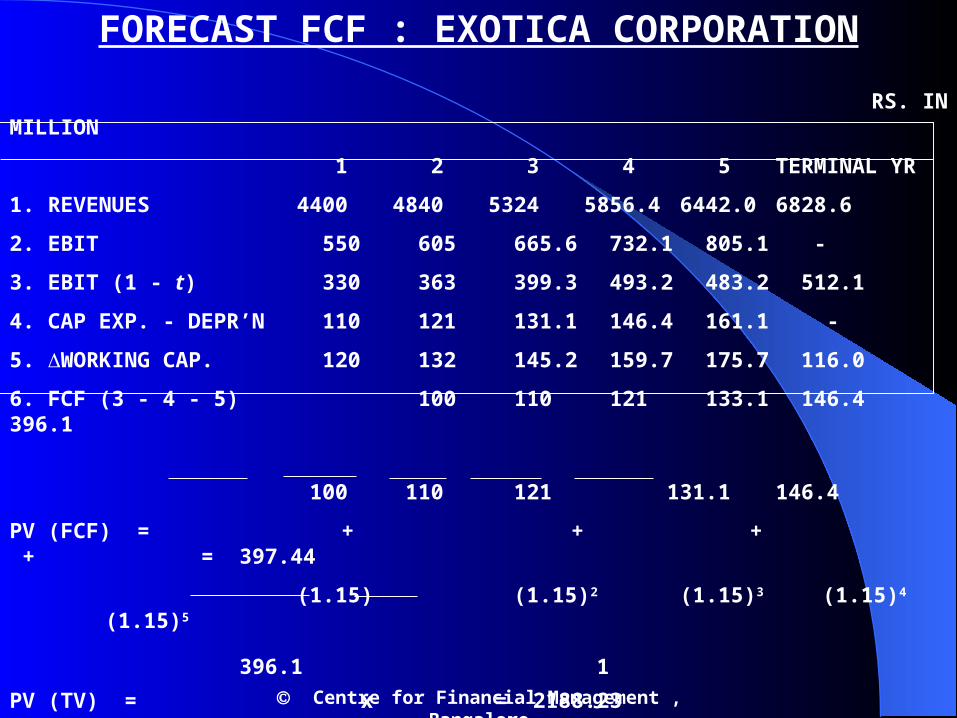
FORECAST FCF : EXOTICA CORPORATION

RS. IN MILLION

1 2 3 4 5 TERMINAL YR

1. REVENUES 4400 4840 5324 5856.4 6442.0 6828.6

2. EBIT 550 605 665.6 732.1 805.1 -

3. EBIT (1 - t) 330 363 399.3 493.2 483.2 512.1

4. CAP EXP. - DEPR’N 110 121 131.1 146.4 161.1 -

5. WORKING CAP. 120 132 145.2 159.7 175.7 116.0

6. FCF (3 - 4 - 5) 100 110 121 133.1 146.4 396.1

100 110 121 131.1 146.4

PV (FCF) = + + + + = 397.44

(1.15) (1.15)2 (1.15)3 (1.15)4 (1.15)5

396.1 1PV (TV) = x = 2188.23

0.15 - 0.06 (1.15)5

FIRM VALUE = 397.44 + 2188.23 = 2585.67 M Centre for Financial Management , Bangalore

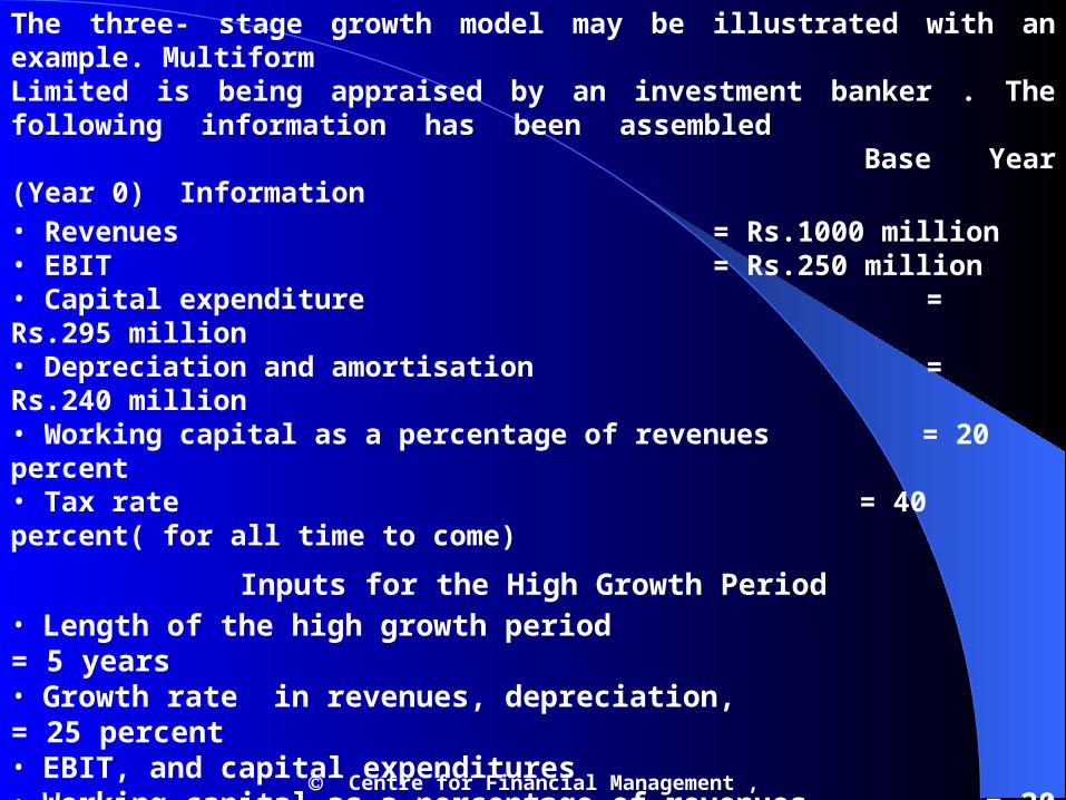
The three- stage growth model may be illustrated with an example. Multiform Limited is being appraised by an investment banker . The following information has been assembled

Base Year (Year 0) Information• Revenues = Rs.1000 million• EBIT = Rs.250 million• Capital expenditure = Rs.295 million• Depreciation and amortisation = Rs.240 million• Working capital as a percentage of revenues = 20 percent• Tax rate = 40 percent( for all time to come)

Inputs for the High Growth Period• Length of the high growth period = 5 years• Growth rate in revenues, depreciation, = 25 percent• EBIT, and capital expenditures• Working capital as a percentage of revenues = 20 percent• Cost of debt = 15 percent (pre-tax)• Debt-equity ratio = 1.5• Risk free rate = 12 percent • Market risk premium = 6 percent• Equity beta = 1.583• WACC= 0.4 [12 + 1.583(6)] + 0.6 [15(1-0.4)] = 14.00 percent


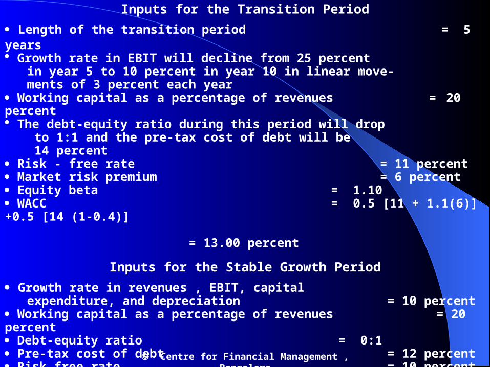
Inputs for the Transition Period Length of the transition period = 5 years Growth rate in EBIT will decline from 25 percent in year 5 to 10 percent in year 10 in linear move- ments of 3 percent each year Working capital as a percentage of revenues = 20 percent The debt-equity ratio during this period will drop to 1:1 and the pre-tax cost of debt will be 14 percent Risk - free rate = 11 percent Market risk premium = 6 percent Equity beta = 1.10 WACC = 0.5 [11 + 1.1(6)] +0.5 [14 (1-0.4)] = 13.00 percent

Inputs for the Stable Growth Period Growth rate in revenues , EBIT, capital expenditure, and depreciation = 10 percent Working capital as a percentage of revenues = 20 percent Debt-equity ratio = 0:1 Pre-tax cost of debt = 12 percent Risk free rate = 10 percent Market risk premium = 6 percent Equity beta = 1.00 WACC = 1.0 [ 10+1 (6)] = 16.00 percent


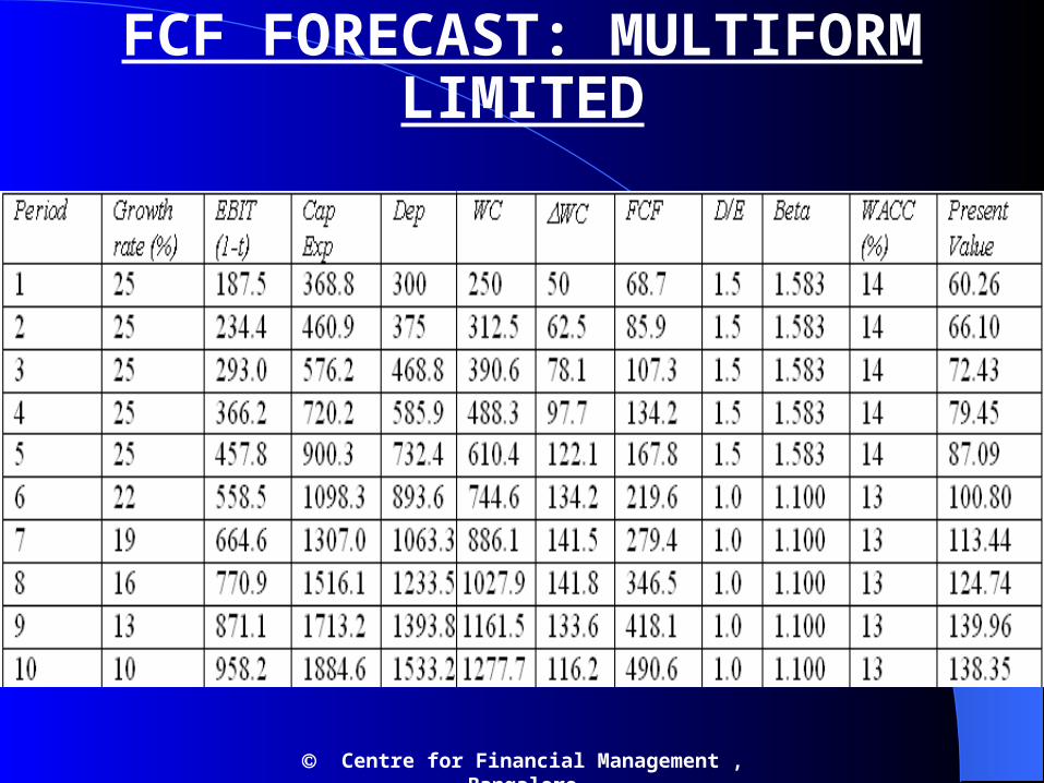
FCF FORECAST: MULTIFORM LIMITED


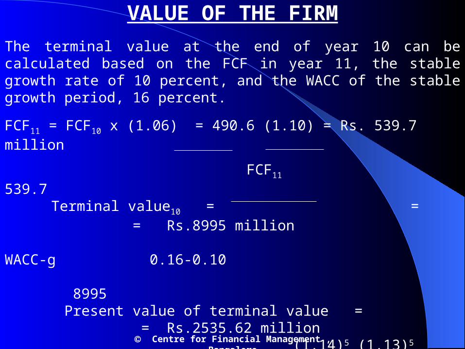
VALUE OF THE FIRMThe terminal value at the end of year 10 can be calculated based on the FCF in year 11, the stable growth rate of 10 percent, and the WACC of the stable growth period, 16 percent.

FCF11 = FCF10 x (1.06) = 490.6 (1.10) = Rs. 539.7 million

FCF11 539.7 Terminal value10 = = = Rs.8995 million WACC-g 0.16-0.10

8995 Present value of terminal value = = Rs.2535.62 million

(1.14)5 (1.13)5

The value of Multiform Limited is arrived at as follows:

Present value of FCF during the high growth period : Rs.365.33 millionPresent value of FCF in the transition period : Rs.617.29 millionPresent value of the terminal value : Rs.2535.62 millionValue of the firm : Rs.3518.24 million



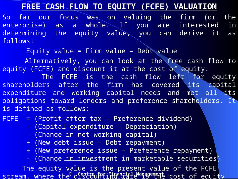
FREE CASH FLOW TO EQUITY (FCFE) VALUATIONSo far our focus was on valuing the firm (or the enterprise) as a whole. If you are interested in determining the equity value, you can derive it as follows:

Equity value = Firm value – Debt value Alternatively, you can look at the free cash flow to equity (FCFE) and discount it at the cost of equity. The FCFE is the cash flow left for equity shareholders after the firm has covered its capital expenditure and working capital needs and met all its obligations toward lenders and preference shareholders. It is defined as follows:FCFE = (Profit after tax – Preference dividend)

- (Capital expenditure – Depreciation)- (Change in net working capital)+ (New debt issue – Debt repayment)+ (New preference issue – Preference repayment)- (Change in investment in marketable securities)

The equity value is the present value of the FCFE stream, where the discounting rate is the cost of equity (rE)

FCFEt

Equity value = (32.4) t=1 (1+ rE)t

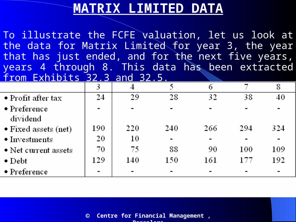
MATRIX LIMITED DATA

To illustrate the FCFE valuation, let us look at the data for Matrix Limited for year 3, the year that has just ended, and for the next five years, years 4 through 8. This data has been extracted from Exhibits 32.3 and 32.5.


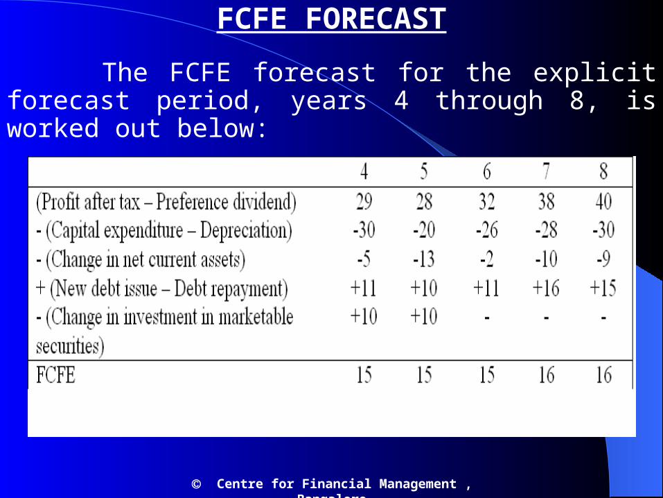
FCFE FORECAST

The FCFE forecast for the explicit forecast period, years 4 through 8, is worked out below:


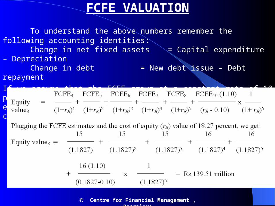
FCFE VALUATION

To understand the above numbers remember the following accounting identities:Change in net fixed assets = Capital expenditure – DepreciationChange in debt = New debt issue – Debt repayment

If we assume that the FCFE grows at a constant rate of 10 percent per year after the explicit forecast period, the equity value using the FCFE valuation method can be calculated as follows:


GUIDELINES FOR VALUATION

1. Understand how the various approaches compare2. Use at least two different approaches3. Work with a value range4. Go behind the numbers5. Value flexibility6. Blend theory with judgment7. Avoid reverse financial engineering8. Beware of possible pitfalls9. Adjust for control premia and non-marketability

factor10.Debunk the myths surrounding valuation


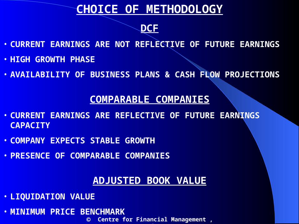
CHOICE OF METHODOLOGYDCF

• CURRENT EARNINGS ARE NOT REFLECTIVE OF FUTURE EARNINGS

• HIGH GROWTH PHASE

• AVAILABILITY OF BUSINESS PLANS & CASH FLOW PROJECTIONS

COMPARABLE COMPANIES• CURRENT EARNINGS ARE REFLECTIVE OF FUTURE EARNINGS

CAPACITY

• COMPANY EXPECTS STABLE GROWTH

• PRESENCE OF COMPARABLE COMPANIES

ADJUSTED BOOK VALUE• LIQUIDATION VALUE

• MINIMUM PRICE BENCHMARK Centre for Financial Management , Bangalore

MYTHS ABOUT VALUATION

1. SINCE VALUATION MODELS ARE QUANTITATIVE, VALUATION IS OBJECTIVE.

2. A GOOD VALUATION PROVIDES A PRECISE ESTIMATE OF VALUE.

3. A WELL-RESEARCHED AND WELL DONE VALUATION IS TIMELESS.

4. THE MARKET IS GENERALLY WRONG.

5. THE PRODUCT OF VALUATION - THE VALUE - IS WHAT MATTERS, THE PROCESS OF VALUATION . . NOT IMP.

6. VALUATION IS AN ART. Centre for Financial Management , Bangalore

SUMMING UP• The IRS of the US has defined fair market value as “ the price at which the property would change hands between a willing buyer and willing seller when the former is not under any compulsion to buy and the latter is not under any compulsion to sell, both the parties having reasonable knowledge of relevant facts”. • There are four broad approaches to appraising the value of a company: adjusted book value approach, stock and debt approach, direct comparison approach, and discounted cash flow approach. • The simplest approach to valuing a company is to rely on the information found on its balance sheet, adjusted for replacement cost or liquidation value.• When the securities of a firm are publicly traded, its value can be obtained by merely adding the market value of all its outstanding securities. This approach is called the stock and debt approach to valuation. • The direct comparison approach involves valuing a company on the basis of how similar companies are valued in the market place.


• The discounted cash flow approach to valuation involves five steps: (a) analysing historical performance, (b) forecasting cash flows, (c) establishing

the cost of capital, (d) determining the continuing value at the end of the explicit forecast period, and (e) calculating the firm value and interpreting results. • There are two simplified versions of the DCF approach which are commonly used: the 2-stage growth model and the 3-stage growth model. • If you are interested in determining the equity value, you can look at the free cash flow to equity (FCFE) and discounting the same at the cost of equity. • The important guidelines that an appraiser should bear in mind while

valuing a company are as follows: (i) Understand how the various approaches compare. (ii) Use at least two different approaches. (iii) Look at a value range. (iv) Go behind the numbers. (v) Value flexibility. (vi) Blend theory with judgment. (vii) Avoid reverse financial engineering. (viii) Beware of possible pitfalls. (ix) Adjust for control premia and non-marketability factor. (x) Debunk the myths surrounding valuation.


chapter32 corporatevaluation

Business