CHAPTER 3

DQPG using AISDistributed query plan generation is an intricate problem has been discussed in Chapter1.

With the number of relations used by query and the number of sites possessing these

relation accessed by query increases. So, the number of generated query plans also gets

increases exponentially. In this dissertation, we are trying to solve distributed query plan

generation problem using AIS as described in chapter 2. DQPG is solved by genetic

algorithm in [VSV11]. But, here an attempt has been taken to solve DQPG using Artificial

Immune System (AIS) as described in Chapter2. A DQPG algorithm has been presented

based on AIS that is used to compute distributed query processing plan for a given

distributed query.

There should be a mapping between original algorithm and AIS. The population of

antibodies is mapped to the query plans in the DQPG and antigens are used as fitness

function in DQPG. The fitness function used in DQPG is treated as antigens. Using this

fitness function, the fitness of antibodies i.e. query plans are computed and query plans

with good fitness are used to make clones in the DQPG. The algorithm is explained in

detail below with the help of an example step by step. Artificial Immune System is similar

to the Genetic Algorithm discussed in evolutionary techniques. This algorithm is inspired

by the human immune system as possessing both antigens and antibodies and adapting the

same process as in the natural immune system. In AIS antibodies are treated as self-bodies

present in the body itself and antigens are assumed as the foreign invaders which cause the

problems to the body. Then antibodies, the part of the immune system encountered with

the foreign agents and finish out those or try to diminish their effect, not only minimise

their effect but also create memory cells to those antibodies in the immune system, so that

if in the future same antigens or similar kind of antigens encountered again in the immune

system then the same antibody will deal with those antigens with greater effect and more

the processed more faster. This is the basic feature of AIS is used in various fields such as

computer securities, multi-modal optimization problems and in text filtering etc.

In this algorithm initially a random population of antibodies are generated. Antibodies are

actually generated by B cells. These antibodies then deal with the antibodies with a certain

affinity and by this way B cells get stimulated. If the level of stimulation is greater than a

threshold value then the that B cell or antibody is chosen for proliferation and used to

make memory cell to serve in the future for the same or similar kind of antigen. But if the

affinity is lower, that antibody dies and excluded from the population. Then the population

with high fitness value is used for the further steps. This process is based on the “Darwin’s

theory of survival of fittest”. This algorithm is adapted to solve DQPG problem which is

earlier solved by genetic algorithm. In DQPG the query plans with less no of sites having

lower QPC values is treated as the more fitter than the query plan having higher value.

This means that to process a query in distributed environment less no of sites are used. So

the time taken to process a query plan with less no of sites is also less. This query plan will

be used in further iterations for further processing. But if the query plan possess a high

QPC value, that query plan is excluded from the set of query plans because it will not give

good results in future. The selected query plans are then chosen to make clones i.e. to

generate certain no of query plans based on its QPC value. This query plan generation of

the selected query plan is based on Roulette Wheel (fitness proportionate function). The

fitness of the new generated query plans is then compared with the existing query plans. If

Contd…

the fitness of newer ones is more, keep those in the original population for future else

discard those. This whole process is flows until an optimum solution is found out or the

condition of the maximum criteria is met. The problem of DQPG is tried to solve by AIS

below.

3.1 DQPG using AIS

3.1.1 MODEL 2

As discussed in Chapter2, AIS is being adapted corresponding to the DQPG problem.

DQPG algorithm based on AIS is shown in Figure 3.1

Input:

RS: Relation-Site matrix, P: Size of antibodies population,Pm: Probability of mutation,GP: Pre-specified number of generations,R: Number of relations to be used in query plan, S: Number of sites to be used containing these relations, β: Clone rate,n: Top query plans with least QPC value to be selected

Output: Top-k Query Plans

Method:

Step1: QP = QueryPlan (RS, P) // Population Initialization phase //Step2: Compute fitness of each antibody query plan in QP

QPC=∑i=1

MSiN (1−Si

N )…………(1)

Step3: Repeat

//Antibody selection phase // Step3.1: Choose top ‘n’ antibody query plans with least QPC value.

//Clone calculation phase// Step3.2: Calculate total number of clones of selected top n query plans using

Cn=Cn+( ( β∗P )i )………… (2)

// Clones division to each query plan// Step3.3: Repeat

Step3.3.1: Calculate number of clones for each selected query plan.

C i=(Z−QPC i)

Z 1 …… (3);

Where

Z1=Z1+( Z−QPC i )… …(3a); Z=(R−1)

R……(3b);

Until i = n

// Clones generation phase of selected antibody query plans //Step3.4: Repeat

Step3.4.1: Compute clones for selected antibody query plans;

Until i = n && j = number of clones of ith antibody query plan

//Antibody query plan mutation phase//Step3.5: Repeat

Step3.5.1: Mutated Clones = Mutation (P, Pm, n, Cn, QPC, Cloned Query Plans);

Until i = number of clones

// New antibodies query plans for next generation // Step3.6: Population = P+ Mutated Clones;

Step3.7: P=Top Query plans of Population

Until Generation=Gp;

Figure 3.1 AIS based DQPG algorithm

Explanation:

AIS based DQPG algorithm is used to generate distributed query plans based on the

property of closeness [VSV11]. The input used by this algorithm are Relation-Site matrix

RS, Population of antibodies, Probability of mutation, Pre-specified number of

generations, Number of relations to be used in query plan, Number of sites to be used

containing these relations, Clone rate, Top query plans with least QPC value. Population

of antibodies is used as input initially, which will be improved by AIS based DQPG over

generations to get fitter populations. One antibody is treated as a query plan and one query

plan is the combination of number of relations and number of sites on which these

relations are present. These query plans are generated with the help of relation-site matrix

randomly.

In the next step, Query Processing Cost of each antibody is calculated present in the

population implies that after the initialization of the population, fitness of query plans is

computed using the fitness function ∑i=1

S S i

N (1− S i

N ) given in [VSV11]. Where S is the

number of times the site is used in the query plan or the other way to define S is that those

sites which contain the relations present in the query plan. N denotes the number of

relations used in the query plan. The Query Plans with less QPC are fitter than the Query

Plans with more QPC. The Query Plan with least QPC is the fittest Query Plan. This step

correlates to the affinity between antigen and antibodies as given in CLONALG explained

in chapter 2 Figure 2. Here affinity corresponds to the fitness of antibody i.e. lower the

QPC value higher is the affinity of antigen and antibody.

After computing fitness of all query plans, select top ‘n’ query plans based on their query

proximity cost (QPC). These selected top ‘n’ query plans are used for further for

calculation of total number of clones based on their fitness value using Cn=∑i=1

n

β∗P / i as

given in []. Here in above equation,β has been used as a parameter that is going to be used

for computation of total number of clones of each selected top ‘n’ query plan and P is the

population of antibody query plans. Roulette Wheel, a Fitness proportionate function that

is used to compute clones of each selected antibody query plan based on the proportion of

Cn value i.e. total number of query plans using C i=(Z−QPC i)

Z 1,a method given in

equation [3]. In above method, Z1=Z1+(Z−QPC i), Z=(R−1)

R, QPC i is the Query

Processing Cost of each ith selected query plan and R is the total no. of relations present in

given query plan. These above methods given in equation [], [], [] are derived using

roulette wheel selection function. Randomly generate number of clones of each selected

ith query plan based on its proportion of the total number of query plans for all ‘n’ query

plans using roulette wheel selection. For this purpose first, random numbers equal to the

total number of clones are computed and then use Roulette wheel selection proportionate

function to generate Clones of these selected ‘n’ query plans.

After generation of clones, Mutation operator from AIS [LJ02] is applied to mutate query

plans. Mutation (P, Pm, n, Cn, QPC, Cloned Query Plans), a function used to apply

mutation on computed clones. Pm a mutation parameter in this model is taken as a

parameter. Here affinity corresponds to the fitness value of query plan i.e. QPC value.

Greater is the fitness value lesser is the mutation for that query plan. Compute QPC of

these mutated query plans and sort mutated query plans based on the QPC value in

ascending order as explained in next section with the help of example. Here mutation is

applied using roulette wheel proportional operator which defines that greater is the QPC

proportion of top ‘n’ query plans in roulette wheel higher will be the mutation rate. The

purpose of inverse relation between fitness of antibody query plan and mutation is that

higher the fitness of the query plans, lesser should be the changes in the query plan.

Because a query plan with higher fitness will be better to pass in the next generation and

vice versa.

After mutation operation, mutated query plans are added in present population ‘P’.

Arrange whole population (P + Mutated Clones) in ascending order on the bases of QPC

value or in other words, arrange in descending order on the basis of fitness of query plans.

After arranging query plans based on fitness value, select top antibody query plans based

on fitness value for next generation population and the size of next generation population

is same as that of the initial population i.e. P.

The step 3 as given in algorithm in Figure 3.1 will be repeated until some stopping

criterion is met such as maximum number of generation reached, optimum solution of the

problem etc. Here in AIS based DQPG algorithm, the stopping criterion used is the

maximum number of generations and the aim of this algorithm to get a superior population

of antibody query plans from the population as taken initially.

3.2 An Example Using AIS based DQPG

Let us take an example to apply AIS based DQPG to explain a distributed query plan. For

this purpose, let us consider a distribute database system with six sites such as S1, S2, S3,

S4, S5 and S6. Let us consider a distributed query accessing six relations such as R1, R2,

R3, R4, R5 and R6.

Select A1, A2, A3

From R1, R2, R3, R4, R5, R6

Where R1.A1=R2.A1 and R3.A2=R4.A2 and R5.A3=R6.A3

Figure 3.2 Relation-Site Matrix

The main objective of this example is to generate top ‘n’ query plans of the total

population for the given distributed query, using AIS based DQPG algorithm. The

relations used in distributed query are accessed from generated relation-site matrix is

shown in Figure 3.2. Relation-site matrix is the combination of the relations and sites,

where relations in matrix are the relations used in distributed query and sites represents

where these relations are present. In relation-site matrix, the value present 1 in cell

indices, indicates the presence of relation on host sites while 0 in relation-site matrix cells

indices indicates the absence of relation on the site.

Now example based on Artificial Immune System.

Input:

Relation * Site matrix of size RX S (6 X 6) Max. No. Of generations ( GP) =2 No. of relations in the query (R) = 6 The size of populations i.e. no. of query plans =10 The value of clone rate (β)

No. of sites used in the distributed query =6 Fraction of query plans to be selected i.e. n=0.4*P

Output: Top 4 query plans.

Step1: Generate Initial Population ‘P’ of antibodies: Use Relation-Site matrix as

explained and shown above in Figure 3.2 to generate 10 antibody (10 query plans).

Generated query plans are shown in Figure 3.3. One query plan can be represented as

X={, x2 , x3 , x4 , x5 , x6 }.

Step 2: Antibody-Antigen affinity Computation: Compute fitness of each antibody query

plans using QPC function given [VSV11]. QPC function is based on the closeness

property as explained in [VSV11]. The query plan with less QPC is treated as more closer

than the query plan with more QPC.

QPC=∑i=1

S S i

N (1− S i

N )The query plan with lower QPC has high fitness than query plan with high QPC. Each

query plan in population with respective QPC is given below in Figure 3.3.

Sr. No. Query Plan QPC

X1 [5,6,4,4,1,2] 0.7778X2 [5,1,2,6,4,4] 0.7778X3 [3,1,1,6,3,2] 0.7222X4 [5,4,4,6,4,4] 0.5000X5 [3,2,2,2,3,1] 0.6111X6 [1,2,4,5,2,4] 0.7222X7 [6,6,2,2,3,4] 0.7222X8 [3,3,1,4,3,4] 0.6111X9 [1,3,6,5,3,1] 0.7222X10 [3,4,4,2,2,4] 0.6111

Figure 3.3 Antibody Query Plans population with respective QPC

Step 3: Generation=1.

Step 3.1: Select top ‘n’ query plans with high fitness: Select ‘n’ Query plans from P with

lower QPC. Here n=0.4*P. So, 4 best query plans will be selected as shown in Figure 3.4.

Sr. No. Query Plans QPCX4 [5,4,4,6,4,4] 0.5000X5 [3,2,2,2,3,1] 0.6111X8 [3,3,1,4,3,4] 0.6111X10 [3,4,4,2,2,4] 0.6111

Figure 3.4 Top ‘n’ query plans with lower QPC

Step3.2: Clone calculation of selected query plans: Compute total number of clones of n1

antibody query plans using equation [] as shown below. Cn Denotes total number of

clones. Here β and α, are the constant parameters are used for clones computation.

Where

Cn=∑i=1

n1

β∗P / i

Here β=α*β; α=0.9; β=0.99.

So, Cn=19.

Step 3.3: i = 1. Here, i has been used as a counter to count top ‘n’ query plans.

Step 3.3.1: Clones distribution phase: Distribute clones to each selected query plan using

method given in []. Compute clones proportion of ith query plan;

C i=(Z−QPC i)

Z 1

The above equation is derived through Roulette Wheel Selection to compute proportion of

each query based on QPC of each Query Plan in ‘n’.

Z1=Z1+( Z−QPC i )

Equation (2) also based on Roulette Wheel is used to computeZ1.

Z=(R−1)

R

Equation (3) gives Z which is used by C i to calculate clones for ‘n’ query plans as shown

below using example.

Ris the number of relations has been used in query plan.

Z=(6−1)

6

⟹ Z = 5/6

⟹Z =0.83

After Z computation, use it to compute Z 1 as shown below in Figure 3.5.

Sr. no. QPC Z -QPC i

1 0.5000 0.33002 0.6111 0.21893 0.6111 0.21894 0.6111 0.2189

Total (Z 1) = 0.9867

Figure 3.5 Z 1 value computation using Roulette Wheel

Computation of proportion of clones for each top ‘n’ query plan is computed below shown

in Figure 3.6 using equation (1).

C i (Z−QPC i)Z 1

0.3345 0.3300/0.98670.2219 0.2189/0.98670.2219 0.2189/0.98670.2219 0.1633/0.9867

Figure 3.6 Clone proportion computation of each query plan in ‘n’

A drawn a pie chart on the bases of clone proportion computation of top ‘n’ query plans

are shown in Figure 3.7

Figure 3.7 Roulette wheel for clones proportion of each selected query plan

Calculate probability of each selected antibody query plan using Roulette Wheel.

Probability chart of each top ‘n’ query plans is shown in Figure 3.8.

1.00020.66570.44380.2219

Figure 3.8 Proportion for each query plans based on QPC value

After probability computation of all top ‘n’ query plans using Roulette Wheel Selection.

Compute random numbers equal to the number of clones. Let us consider, the list of

random numbers generated and clones of corresponding query plan as shown in Figure

3.9.

Random number

Clones for respectivequery plan based on QPC value

0.8147 [5,4,4,6,4,4]0.9058 [5,4,4,6,4,4]0.1270 [3,4,4,2,2,4]0.9134 [5,4,4,6,4,4]0.6324 [3,2,2,2,3,1]0.0975 [3,4,4,2,2,4]0.2785 [3,4,4,2,2,4]0.5469 [3,3,1,4,3,4]0.9575 [5,4,4,6,4,4]0.9649 [5,4,4,6,4,4]0.1576 [3,4,4,2,2,4]0.9706 [5,4,4,6,4,4]0.6787 [3,2,2,2,3,1]0.7577 [3,2,2,2,3,1]0.7431 [3,2,2,2,3,1]0.3922 [3,3,1,4,3,4]0.6555 [3,2,2,2,3,1]0.1712 [3,4,4,2,2,4]0.7060 [3,2,2,2,3,1]

Figure3.9 Clones of top ‘n’ selected query plans based on its probability

Step 3.4: Antibody query plan Mutation Phase: For each clone of i=1 to Cn

Step 3.4.1: Use Roulette Wheel algorithm as explained in MODEL for mutation. For

mutation, first compute a pie chart on the basis of probability of Query plan Processing

Cost of top ‘n’ query plans as shown in Figure 3.10, Figure 3.11 and Figure 3.12

respectively.

Figure 3.10 Probability pie chart for QPC of ‘n’ query plans

QPC Probability0.5000/2.3333 0.21430.6111/2.3333 0.26190.6111/2.3333 0.26190.6111/2.3333 0.2619

Sum 1.0000

Figure 3.11 Probability of selection of query plan

Figure 3.12 Probability of QPC value of ‘n’ selected Query Plans

Computed random numbers equal to the total numbers of clones between 0 and 1.

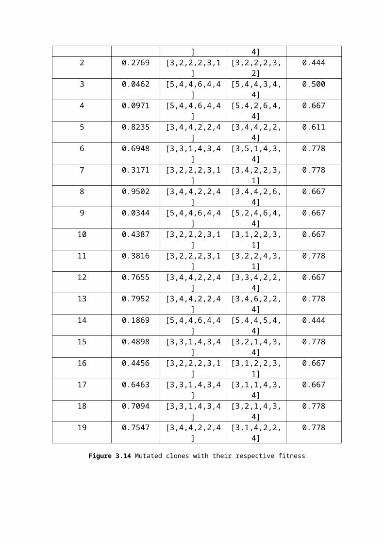
Mutation rate (M R=0.1) shown in Figure 3.13.

Sr. No.(new) Random Number

Query Plan Mutated Query Plan

QPC

1 0.0318 [5,4,4,6,4,4] [5,4,4,6,4,4] 0.5002 0.2769 [3,2,2,2,3,1] [3,2,2,2,3,2] 0.4443 0.0462 [5,4,4,6,4,4] [5,4,4,3,4,4] 0.5004 0.0971 [5,4,4,6,4,4] [5,4,2,6,4,4] 0.6675 0.8235 [3,4,4,2,2,4] [3,4,4,2,2,4] 0.6116 0.6948 [3,3,1,4,3,4] [3,5,1,4,3,4] 0.7787 0.3171 [3,2,2,2,3,1] [3,4,2,2,3,1] 0.7788 0.9502 [3,4,4,2,2,4] [3,4,4,2,6,4] 0.6679 0.0344 [5,4,4,6,4,4] [5,2,4,6,4,4] 0.66710 0.4387 [3,2,2,2,3,1] [3,1,2,2,3,1] 0.66711 0.3816 [3,2,2,2,3,1] [3,2,2,4,3,1] 0.77812 0.7655 [3,4,4,2,2,4] [3,3,4,2,2,4] 0.66713 0.7952 [3,4,4,2,2,4] [3,4,6,2,2,4] 0.77814 0.1869 [5,4,4,6,4,4] [5,4,4,5,4,4] 0.444

1.0000.73810.47620.2143

15 0.4898 [3,3,1,4,3,4] [3,2,1,4,3,4] 0.77816 0.4456 [3,2,2,2,3,1] [3,1,2,2,3,1] 0.66717 0.6463 [3,3,1,4,3,4] [3,1,1,4,3,4] 0.66718 0.7094 [3,3,1,4,3,4] [3,2,1,4,3,4] 0.77819 0.7547 [3,4,4,2,2,4] [3,1,4,2,2,4] 0.778

Figure 3.14 Mutated clones with their respective fitness

Step3.5: Population generation for next generation: Add mutated clones Cn to the

existing population P.

Sr. No. Query Plan QPC1 [5,4,4,6,4,4] 0.5002 [3,2,2,2,3,2] 0.4443 [5,4,4,3,4,4] 0.5004 [5,4,2,6,4,4] 0.6675 [3,4,4,2,2,4] 0.6116 [3,5,1,4,3,4] 0.7787 [3,4,2,2,3,1] 0.7788 [3,4,4,2,6,4] 0.6679 [5,2,4,6,4,4] 0.66710 [3,1,2,2,3,1] 0.66711 [3,2,2,4,3,1] 0.77812 [3,3,4,2,2,4] 0.66713 [3,4,6,2,2,4] 0.77814 [5,4,4,5,4,4] 0.44415 [3,2,1,4,3,4] 0.77816 [3,1,2,2,3,1] 0.66717 [3,1,1,4,3,4] 0.66718 [3,2,1,4,3,4] 0.77819 [3,1,4,2,2,4] 0.77820 [5,6,4,4,1,2] 0.77821 [5,1,2,6,4,4] 0.77822 [3,1,1,6,3,2] 0.72223 [5,4,4,6,4,4] 0.50024 [3,2,2,2,3,1] 0.61125 [1,2,4,5,2,4] 0.72226 [6,6,2,2,3,4] 0.72227 [3,3,1,4,3,4] 0.61128 [1,3,6,5,3,1] 0.72229 [3,4,4,2,2,4] 0.611

Figure 3.15 Combination of Mutated clones and existing population

Step 3.6 Population selection for next generation: Choose new population from above

computed population on the basis of fitness of antibody query plans. The size of new

chosen population is same as of the existing population i.e. ‘P’. The new population for

next generation is shown below in Figure 3.16.

Sr. No. (New) Query Plan QPCX1 [5,4,4,6,4,4] 0.500X2 [3,2,2,2,3,2] 0.444X3 [5,4,4,3,4,4] 0.500X4 [5,4,4,5,4,4] 0.444X5 [5,4,4,6,4,4] 0.500X6 [3,4,4,2,2,4] 0.611X7 [3,2,2,2,3,1] 0.611X8 [3,3,1,4,3,4] 0.611X9 [3,4,4,2,2,4] 0.611X10 [5,4,2,6,4,4] 0.667

Figure 3.16 Population for next generation of size ‘P’

Step3.8: Repeat above step 3 for next Generation: Generation = Generation + 1.

Repeat Step3 for Generation=2

Step3.1: Select top ‘n’ query plans with high fitness: Selected Top ‘n’ query plans are

shown below in Figure 3.17 on the bases of QPC.

Sr. No. (New) Query Plan QPCX2 [3,2,2,2,3,2] 0.444X4 [5,4,4,5,4,4] 0.444X1 [5,4,4,6,4,4] 0.500X3 [5,4,4,3,4,4] 0.500

Figure 3.17 Selected Top ‘n’ query plan for 2nd Generation

Step 3.2: Clone calculation of selected query plans: Compute Cn clones of n1 antibodies

using QPC as shown below. These are the total no of clones generated using n1 selected

antibodies.

Where

Cn=∑i=1

n1

β∗ j / i

Here β=α*β and j=P and α=0.9 and β=0.99.

Cn=19

Step 3.3: i = 1. Here, i has been used as a counter to count top ‘n’ query plans.

Step 3.3.1: Clones distribution phase: Distribute clones to each selected query plan using

method given in []. Compute clones proportion of ith query plan;

C i=(Z−QPC i)

Z 1

The above equation is derived through Roulette Wheel Selection to compute proportion of

each query based on QPC of each Query Plan in ‘n’.

Z1=Z1+( Z−QPC i )

Equation (2) also based on Roulette Wheel is used to computeZ1.

Z=(R−1)

R

Equation (3) gives Z which is used by C i to calculate clones for ‘n’ query plans as shown

below using example.

Ris the number of relations has been used in query plan.

Z=(6−1)

6

⟹ Z = 5/6

⟹Z =0.83

After Z computation, use it to compute Z 1 as shown below in Figure 3.18.

Sr. no. QPC Z-QPC(i)1 0.444 0.3862 0.444 0.3863 0.500 0.3304 0.500 0.330 Total (Z1) = 1.432

Figure 3.18 Z 1 value computation using Roulette Wheel

Computation of proportion of clones for each top ‘n’ query plan is computed below shown

in Figure 3.19 using equation (1).

C i (Z−QPC i)Z 1

0.27

0.386/1.432

0.27

0.386/1.432

0.23

0.330/1.432

0.23

0.330/1.432

Figure 3.19 Clone proportion computation of each query plan in ‘n’

A drawn a pie chart on the bases of clone proportion computation of top ‘n’ query plans

are shown in Figure 3.20

Figure 3.20 Roulette wheel for clones proportion of each selected query plan

Calculate probability of each selected antibody query plan using Roulette Wheel.

Probability chart of each top ‘n’ query plans is shown in Figure 3.21.

Figure 3.21 Proportion for each query plans based on QPC value

After probability computation of all top ‘n’ query plans using Roulette Wheel Selection.

Compute random numbers equal to the number of clones. Let us consider, the list of

random numbers generated and clones of corresponding query plan as shown in Figure

3.22.

Random number

Clones for respectivequery plan based on QPC value

0.9595 [5,4,4,3,4,4]0.6557 [5,4,4,6,4,4]0.0357 [3,2,2,2,3,2]0.8491 [5,4,4,3,4,4]0.9340 [5,4,4,3,4,4]0.6787 [5,4,4,6,4,4]0.7577 [5,4,4,6,4,4]0.7431 [5,4,4,6,4,4]0.3922 [5,4,4,5,4,4]0.6555 [5,4,4,6,4,4]0.1712 [3,2,2,2,3,2]0.7060 [5,4,4,6,4,4]0.0318 [3,2,2,2,3,2]0.2769 [5,4,4,5,4,4]0.0462 [3,2,2,2,3,2]0.0971 [3,2,2,2,3,2]0.8235 [5,4,4,3,4,4]0.6948 [5,4,4,6,4,4]0.3171 [5,4,4,5,4,4]

Figure3.22 Clones of top ‘n’ selected query plans based on its probability

Step 3.4: Antibody query plan Mutation Phase: For each clone of i=1 to Cn

Step 3.4.1: Use Roulette Wheel algorithm as explained in MODEL for mutation. For

mutation, first compute a pie chart on the basis of probability of Query plan Processing

Cost of top ‘n’ query plans as shown in Figure 3.23, Figure 3.24 and Figure 3.25

respectively.

1.000.770.540.27

Figure 3.23 Probability pie chart for QPC of ‘n’ query plans

QPC proportion0.444/1.888 0.2350.444/1.888 0.2350.500/1.888 0.2650.500/1.888 0.265

Sum 1.0000

Figure 3.24 Probability of selection of query plan

Figure 3.25 Probability of QPC value of ‘n’ selected Query Plans

Computed random numbers equal to the total numbers of clones between 0 and 1.

Mutation rate (M R=0.1) shown in Figure 3.26.

Sr. No.(new) Random Number

Query Plan Mutated Query Plan

QPC

1 0.9502 [5,4,4,3,4,4] [5,4,4,6,4,4] 0.5002 0.0344 [3,2,2,2,3,2] [3,2,2,2,3,2] 0.4443 0.4387 [5,4,4,5,4,4] [5,4,4,6,4,4] 0.5004 0.3816 [5,4,4,5,4,4] [5,4,2,5,4,4] 0.6115 0.7655 [5,4,4,3,4,4] [3,4,4,3,4,4] 0.4446 0.7952 [5,4,4,3,4,4] [5,4,1,3,4,4] 0.6677 0.1869 [3,2,2,2,3,2] [3,4,2,2,3,2] 0.6118 0.4898 [5,4,4,6,4,4] [3,4,4,6,4,4] 0.5009 0.4456 [5,4,4,5,4,4] [5,2,4,5,4,4] 0.61110 0.6463 [5,4,4,6,4,4] [5,4,4,5,4,4] 0.44411 0.7094 [5,4,4,6,4,4] [5,4,1,6,4,4] 0.61112 0.7547 [5,4,4,3,4,4] [5,4,4,3,4,2] 0.61113 0.2760 [5,4,4,5,4,4] [5,4,4,1,4,4] 0.50014 0.6797 [5,4,4,6,4,4] [5,4,4,5,4,4] 0.44415 0.6551 [5,4,4,6,4,4] [5,1,4,6,4,4] 0.61116 0.1626 [3,2,2,2,3,2] [3,1,2,2,3,2] 0.61117 0.1190 [3,2,2,2,3,2] [3,2,1,2,3,2] 0.667

1.0000.7350.4700.235

18 0.4984 [5,4,4,6,4,4] [5,2,4,6,4,4] 0.66719 0.9597 [5,4,4,3,4,4] [5,4,1,3,4,4] 0.667

Figure 3.26 Mutated clones with their respective fitness

Step3.5: Population generation for next generation: Add mutated clones Cn to the

existing population P.

Sr. No. Query Plan QPC1 [5,4,4,6,4,4] 0.5002 [3,2,2,2,3,2] 0.4443 [5,4,4,3,4,4] 0.5004 [5,4,4,5,4,4] 0.4445 [5,4,4,6,4,4] 0.5006 [3,4,4,2,2,4] 0.6117 [3,2,2,2,3,1] 0.6118 [3,3,1,4,3,4] 0.6119 [3,4,4,2,2,4] 0.61110 [5,4,2,6,4,4] 0.66711 [5,4,4,6,4,4] 0.50012 [3,2,2,2,3,2] 0.44413 [5,4,4,6,4,4] 0.50014 [5,4,2,5,4,4] 0.61115 [3,4,4,3,4,4] 0.44416 [5,4,1,3,4,4] 0.66717 [3,4,2,2,3,2] 0.61118 [3,4,4,6,4,4] 0.50019 [5,2,4,5,4,4] 0.61120 [5,4,4,5,4,4] 0.44421 [5,4,1,6,4,4] 0.61122 [5,4,4,3,4,2] 0.61123 [5,4,4,1,4,4] 0.50024 [5,4,4,5,4,4] 0.44425 [5,1,4,6,4,4] 0.61126 [3,1,2,2,3,2] 0.61127 [3,2,1,2,3,2] 0.66728 [5,2,4,6,4,4] 0.66729 [5,4,1,3,4,4] 0.667

Figure 3.27 Combination of Mutated clones and existing population

Step 3.6 Population selection for next generation: Choose new population from above

computed population on the basis of fitness of antibody query plans. The size of new

chosen population is same as of the existing population i.e. ‘P’. The new population for

next generation is shown below in Figure 3.28.

Sr. No. (New) Query Plan QPCX1 [5,4,4,6,4,4] 0.500X2 [3,2,2,2,3,2] 0.444X3 [5,4,4,3,4,4] 0.500X4 [5,4,4,5,4,4] 0.444X5 [5,4,4,6,4,4] 0.500X6 [3,4,4,2,2,4] 0.611X7 [3,2,2,2,3,1] 0.611X8 [3,3,1,4,3,4] 0.611X9 [3,4,4,2,2,4] 0.611X10 [5,4,2,6,4,4] 0.667

Figure 3.28 Population for next generation of size ‘P’

Step 3.8: Repeat above step 3 for next Generation: Generation = Generation + 1 and

repeat ‘Step3’ until some stopping criterion is met. Stopping criterion taken in this

example is maximum number of generations.

Step4: End.