chapter8 qcdin e annihilations - eth zedu.itp.phys.ethz.ch/hs10/ppp1/ppp1_8.pdf · 158 chapter 8....
TRANSCRIPT
Chapter 8
QCD in e+e− annihilations
Literature:
• Dissertori/Knowles/Schmelling [27]
• Ellis/Stirling/Webber [28]
• Bethke [29, 30]
• Particle Data Group [26]
• JADE, Durham, and Cambridge jet algorithms [31, 32, 33, 34]
• FastJet Package, Fast kT , SISCone [35, 36, 37]
In Chap. 7, QCD is introduced as an SU(3) gauge theory. Here we continue this discus-sion and consider QCD processes following e+e− annihilations. The main focus is on thedefinition and application of observables linking theoretical predictions with measurablequantities: Jets and event shapes are discussed; the applications include measurements ofthe parton spins, the strong coupling constant, and the QCD color factors. The chapteris concluded by an outlook to hadronization and non-perturbative QCD.
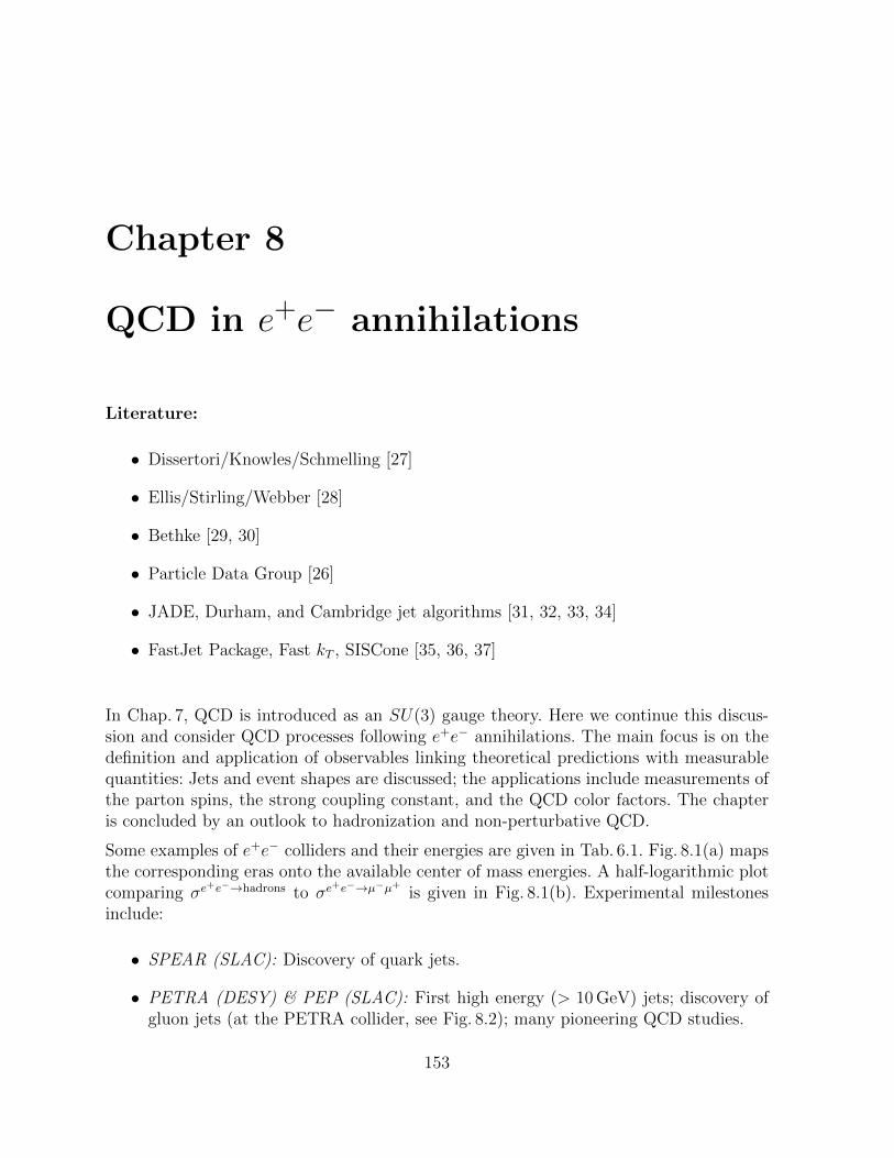
Some examples of e+e− colliders and their energies are given in Tab. 6.1. Fig. 8.1(a) mapsthe corresponding eras onto the available center of mass energies. A half-logarithmic plotcomparing σe
+e−→hadrons to σe+e−→µ−µ+
is given in Fig. 8.1(b). Experimental milestonesinclude:
• SPEAR (SLAC): Discovery of quark jets.
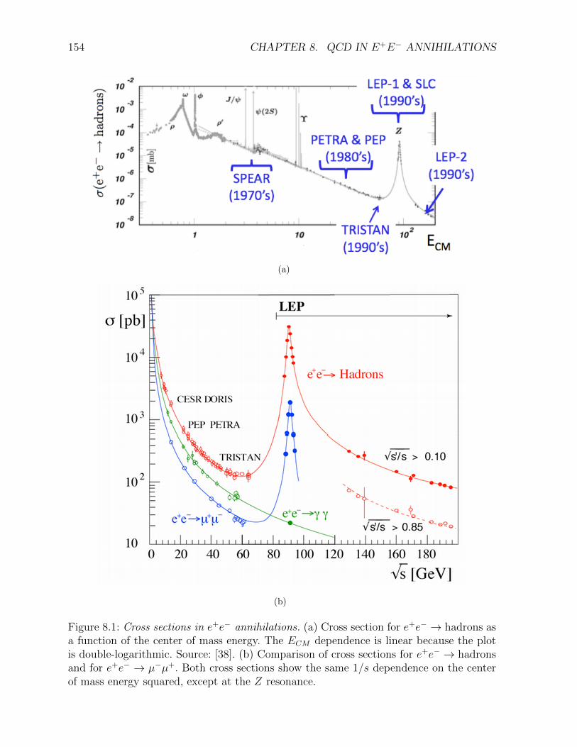
• PETRA (DESY) & PEP (SLAC): First high energy (> 10GeV) jets; discovery ofgluon jets (at the PETRA collider, see Fig. 8.2); many pioneering QCD studies.
153
154 CHAPTER 8. QCD IN E+E− ANNIHILATIONS
(a)
���������������������������� �����
(b)
Figure 8.1: Cross sections in e+e− annihilations. (a) Cross section for e+e− → hadrons asa function of the center of mass energy. The ECM dependence is linear because the plotis double-logarithmic. Source: [38]. (b) Comparison of cross sections for e+e− → hadronsand for e+e− → µ−µ+. Both cross sections show the same 1/s dependence on the centerof mass energy squared, except at the Z resonance.
8.1. THE BASIC PROCESS: E+E− → QQ̄ 155
(a) (b)
Figure 8.2: Gluon discovery at the PETRA collider at DESY, Hamburg. Event display (a)and reconstruction (b).
• LEP (CERN) & SLC (SLAC): Large energies (small αs, see later) mean more re-liable calculations and smaller hadronization uncertainties. Large data samples arecollected: ∼ 3 ·106 hadronic Z decays per experiment. This allows for precision testsof QCD.
8.1 The basic process: e+e− → qq̄
In Sect. 5.10 we calculated the cross section for e+e− → µ+µ− and found
σe+e−→µ+µ−
=4πα2em3s
=86.9 nbGeV2
s(8.1)
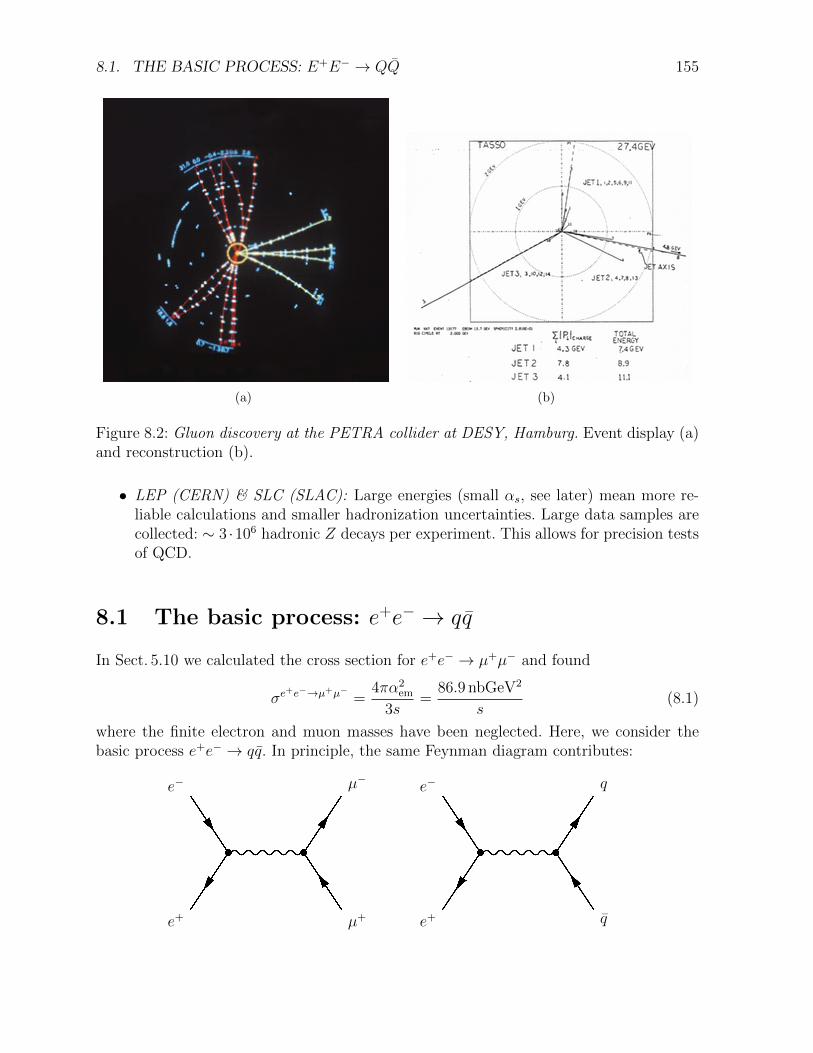
where the finite electron and muon masses have been neglected. Here, we consider thebasic process e+e− → qq̄. In principle, the same Feynman diagram contributes:
�e+
e−
µ+
µ−
�e+
e−
q̄
q
156 CHAPTER 8. QCD IN E+E− ANNIHILATIONS
The only differences are the fractional electric charges of the quarks and the fact that thequarks appear in Nc = 3 different colors which cannot be distinguished by measurement.Therefore, the cross section is increased by a factor Nc. For the quark-antiquark case onethus finds (for mq = 0)
σe+e−→qq̄0 =
4πα2em3s
e2qNc =86.9 nbGeV2
se2qNc. (8.2)
We assume�
q σe+e−→qq̄ = σe
+e−→hadrons, i. e. the produced quark-antiquark pair willalways hadronize.
With Eq. (8.1) and (8.2), neglecting mass effects and gluon as well as photon radiation,we find the following ratio:
R =σe
+e−→hadrons
σe+e−→µ+µ− = Nc
�
q
e2q. (8.3)
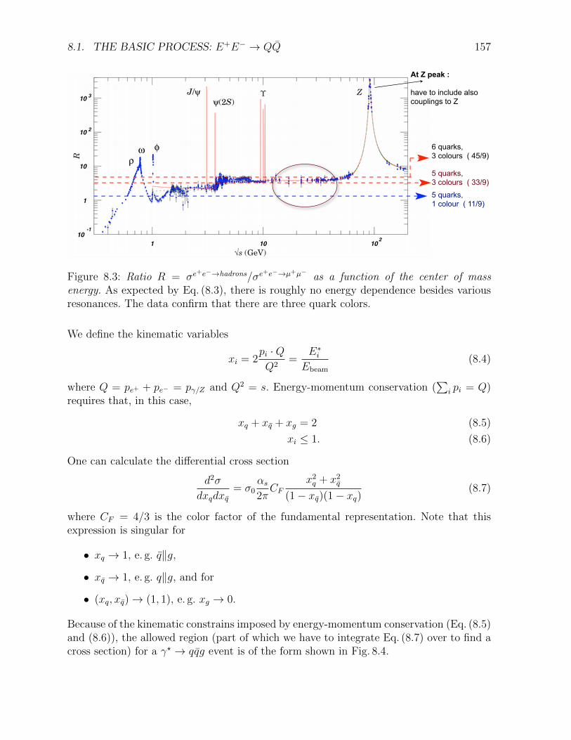
The sum runs over all flavors that can be produced at the available energy. For ECM
below the Z peak and above the Υ resonance (see Fig. 8.3), we expect1
R = Nc
�
q
e2q = Nc
�2
3
�2
� �� �u
+
�
−1
3
�2
� �� �d
+
�
−1
3
�2
� �� �s
+
�2
3
�2
� �� �c
+
�
−1
3
�2
� �� �b
= Nc
11
9.
This is in good agreement with the data for Nc = 3 which confirms that there are threecolors. At the Z peak one also has to include coupling to the Z boson which can be createdfrom the e+e− pair instead of a photon. The small remaining difference visible in the plotis because of QCD corrections for gluon radiation (see later).
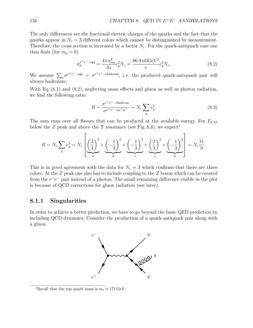
8.1.1 Singularities
In order to achieve a better prediction, we have to go beyond the basic QED prediction byincluding QCD dynamics: Consider the production of a quark-antiquark pair along witha gluon:
�e+
e−
q̄
g
q
1Recall that the top quark mass is mt ≈ 171GeV.
8.1. THE BASIC PROCESS: E+E− → QQ̄ 157
�
������������������������������������������
����������������������������
����������������������������
���������������������������
�����������
�����������������������������������
Figure 8.3: Ratio R = σe+e−→hadrons/σe
+e−→µ+µ−as a function of the center of mass
energy. As expected by Eq. (8.3), there is roughly no energy dependence besides variousresonances. The data confirm that there are three quark colors.
We define the kinematic variables
xi = 2pi ·Q
Q2=
E∗i
Ebeam(8.4)
where Q = pe+ + pe− = pγ/Z and Q2 = s. Energy-momentum conservation (�
i pi = Q)requires that, in this case,
xq + xq̄ + xg = 2 (8.5)
xi ≤ 1. (8.6)
One can calculate the differential cross section
d2σ
dxqdxq̄= σ0
αs
2πCF
x2q + x2q̄(1− xq̄)(1− xq)
(8.7)
where CF = 4/3 is the color factor of the fundamental representation. Note that thisexpression is singular for
• xq → 1, e. g. q̄�g,
• xq̄ → 1, e. g. q�g, and for
• (xq, xq̄)→ (1, 1), e. g. xg → 0.
Because of the kinematic constrains imposed by energy-momentum conservation (Eq. (8.5)and (8.6)), the allowed region (part of which we have to integrate Eq. (8.7) over to find across section) for a γ� → qq̄g event is of the form shown in Fig. 8.4.
158 CHAPTER 8. QCD IN E+E− ANNIHILATIONS
q q̄
q q̄q q̄
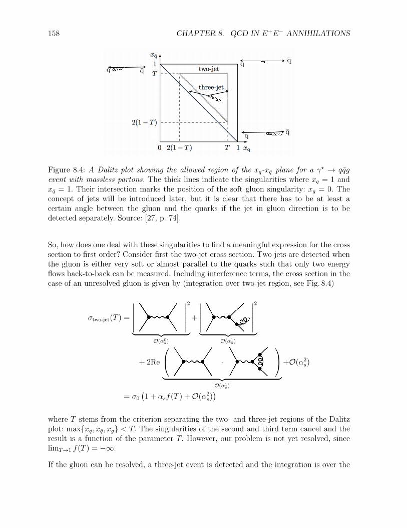
Figure 8.4: A Dalitz plot showing the allowed region of the xq-xq̄ plane for a γ� → qq̄gevent with massless partons. The thick lines indicate the singularities where xq = 1 andxq̄ = 1. Their intersection marks the position of the soft gluon singularity: xg = 0. Theconcept of jets will be introduced later, but it is clear that there has to be at least acertain angle between the gluon and the quarks if the jet in gluon direction is to bedetected separately. Source: [27, p. 74].
So, how does one deal with these singularities to find a meaningful expression for the crosssection to first order? Consider first the two-jet cross section. Two jets are detected whenthe gluon is either very soft or almost parallel to the quarks such that only two energyflows back-to-back can be measured. Including interference terms, the cross section in thecase of an unresolved gluon is given by (integration over two-jet region, see Fig. 8.4)
σtwo-jet(T ) =
�������
������
2
� �� �O(α0
s)
+
�������
������
2
� �� �O(α1
s)
+ 2Re
� ·�
� �� �O(α1
s)
+O(α2s)
= σ0�1 + αsf(T ) +O(α2s)
�
where T stems from the criterion separating the two- and three-jet regions of the Dalitzplot: max{xq, xq̄, xg} < T. The singularities of the second and third term cancel and theresult is a function of the parameter T. However, our problem is not yet resolved, sincelimT→1 f(T ) = −∞.
If the gluon can be resolved, a three-jet event is detected and the integration is over the
8.2. JETS AND OTHER OBSERVABLES 159
(a) (b)
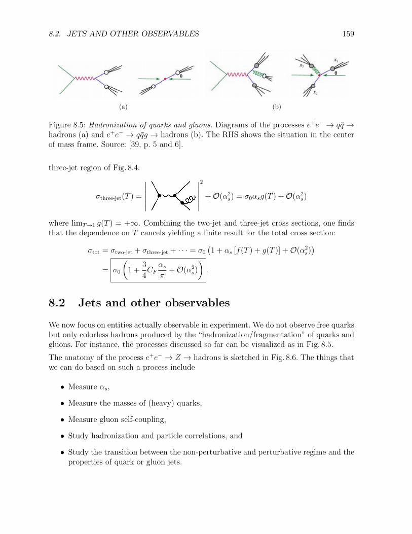
Figure 8.5: Hadronization of quarks and gluons. Diagrams of the processes e+e− → qq̄ →hadrons (a) and e+e− → qq̄g → hadrons (b). The RHS shows the situation in the centerof mass frame. Source: [39, p. 5 and 6].
three-jet region of Fig. 8.4:
σthree-jet(T ) =
�������
������
2
+O(α2s) = σ0αsg(T ) +O(α2s)
where limT→1 g(T ) = +∞. Combining the two-jet and three-jet cross sections, one findsthat the dependence on T cancels yielding a finite result for the total cross section:
σtot = σtwo-jet + σthree-jet + · · · = σ0�1 + αs [f(T ) + g(T )] +O(α2s)
�
= σ0
�
1 +3
4CF
αs
π+O(α2s)
�
.
8.2 Jets and other observables
We now focus on entities actually observable in experiment. We do not observe free quarksbut only colorless hadrons produced by the “hadronization/fragmentation” of quarks andgluons. For instance, the processes discussed so far can be visualized as in Fig. 8.5.
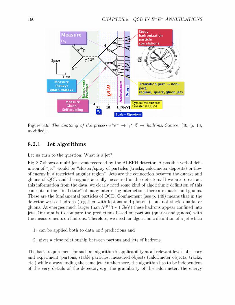
The anatomy of the process e+e− → Z → hadrons is sketched in Fig. 8.6. The things thatwe can do based on such a process include
• Measure αs,
• Measure the masses of (heavy) quarks,
• Measure gluon self-coupling,
• Study hadronization and particle correlations, and
• Study the transition between the non-perturbative and perturbative regime and theproperties of quark or gluon jets.
160 CHAPTER 8. QCD IN E+E− ANNIHILATIONS
Figure 8.6: The anatomy of the process e+e− → γ�, Z → hadrons. Source: [40, p. 13,modified].
8.2.1 Jet algorithms
Let us turn to the question: What is a jet?
Fig. 8.7 shows a multi-jet event recorded by the ALEPH detector. A possible verbal defi-nition of “jet” would be “cluster/spray of particles (tracks, calorimeter deposits) or flowof energy in a restricted angular region”. Jets are the connection between the quarks andgluons of QCD and the signals actually measured in the detectors. If we are to extractthis information from the data, we clearly need some kind of algorithmic definition of thisconcept: In the “final state” of many interesting interactions there are quarks and gluons.These are the fundamental particles of QCD. Confinement (see p. 148) means that in thedetector we see hadrons (together with leptons and photons), but not single quarks orgluons. At energies much larger than ΛQCD(∼ 1GeV) these hadrons appear confined intojets. Our aim is to compare the predictions based on partons (quarks and gluons) withthe measurements on hadrons. Therefore, we need an algorithmic definition of a jet which
1. can be applied both to data and predictions and
2. gives a close relationship between partons and jets of hadrons.
The basic requirement for such an algorithm is applicability at all relevant levels of theoryand experiment: partons, stable particles, measured objects (calorimeter objects, tracks,etc.) while always finding the same jet. Furthermore, the algorithm has to be independentof the very details of the detector, e. g. the granularity of the calorimeter, the energy

8.2. JETS AND OTHER OBSERVABLES 161
Figure 8.7: Multi-jet event in the ALEPH detector.
response, etc. Finally, it should also be easy to implement. In order that we can testQCD predictions, there has to be a close correspondence between the jet momentum (i. e.energy, momentum, and angle) at the parton level and at the hadron level.
NB: Other requirements might strongly depend on the specific applica-tion/measurement being performed: For a precision test of QCD there may berequirements which for an analysis of W decays or searches for new physics might not benecessary (e. g. infrared safety).
Further requirements come from QCD: We want to compare perturbative calculationswith the data. Therefore, the algorithm has to be insensitive to “soft physics” whichrequires infrared safety and collinear safety.
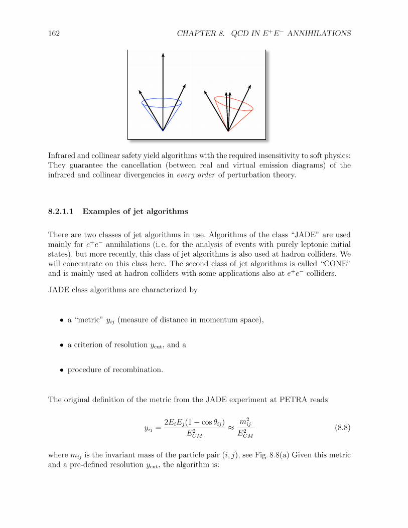
Infrared safety requires that the configuration must not change when adding a furthersoft particle. This would be violated by the following behavior2:
Collinear safety means that the configuration does not change when substituting oneparticle with two collinear particles. The problem is visualized in this figure:
2Source: [41, pp. 4].
162 CHAPTER 8. QCD IN E+E− ANNIHILATIONS
Infrared and collinear safety yield algorithms with the required insensitivity to soft physics:They guarantee the cancellation (between real and virtual emission diagrams) of theinfrared and collinear divergencies in every order of perturbation theory.
8.2.1.1 Examples of jet algorithms
There are two classes of jet algorithms in use. Algorithms of the class “JADE” are usedmainly for e+e− annihilations (i. e. for the analysis of events with purely leptonic initialstates), but more recently, this class of jet algorithms is also used at hadron colliders. Wewill concentrate on this class here. The second class of jet algorithms is called “CONE”and is mainly used at hadron colliders with some applications also at e+e− colliders.
JADE class algorithms are characterized by
• a “metric” yij (measure of distance in momentum space),
• a criterion of resolution ycut, and a
• procedure of recombination.
The original definition of the metric from the JADE experiment at PETRA reads
yij =2EiEj(1− cos θij)
E2CM≈
m2ijE2CM
(8.8)
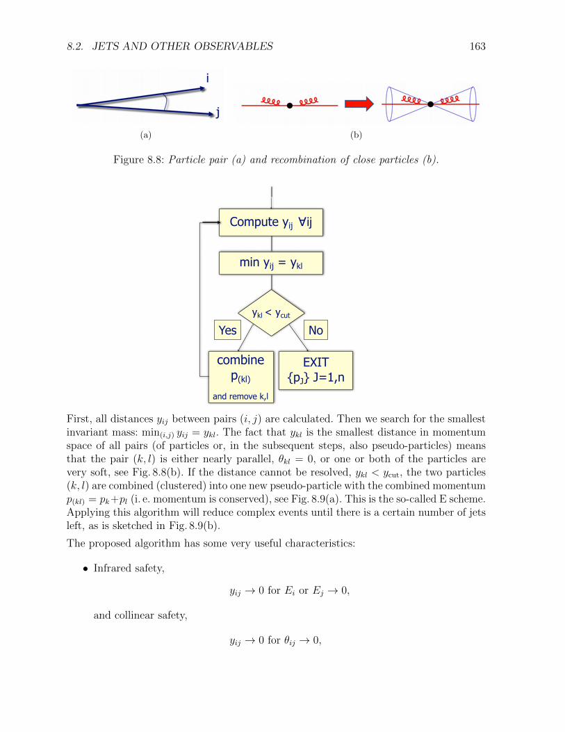
where mij is the invariant mass of the particle pair (i, j), see Fig. 8.8(a) Given this metricand a pre-defined resolution ycut, the algorithm is:
8.2. JETS AND OTHER OBSERVABLES 163
(a) (b)
Figure 8.8: Particle pair (a) and recombination of close particles (b).
����������������
�������������
����������
��������������
��������������
��������������
�����
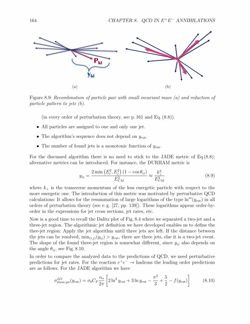
First, all distances yij between pairs (i, j) are calculated. Then we search for the smallestinvariant mass: min(i,j) yij = ykl. The fact that ykl is the smallest distance in momentumspace of all pairs (of particles or, in the subsequent steps, also pseudo-particles) meansthat the pair (k, l) is either nearly parallel, θkl = 0, or one or both of the particles arevery soft, see Fig. 8.8(b). If the distance cannot be resolved, ykl < ycut, the two particles(k, l) are combined (clustered) into one new pseudo-particle with the combined momentump(kl) = pk+pl (i. e. momentum is conserved), see Fig. 8.9(a). This is the so-called E scheme.Applying this algorithm will reduce complex events until there is a certain number of jetsleft, as is sketched in Fig. 8.9(b).
The proposed algorithm has some very useful characteristics:
• Infrared safety,
yij → 0 for Ei or Ej → 0,
and collinear safety,
yij → 0 for θij → 0,
164 CHAPTER 8. QCD IN E+E− ANNIHILATIONS
���
���
(a) (b)
Figure 8.9: Recombination of particle pair with small invariant mass (a) and reduction ofparticle pattern to jets (b).
(in every order of perturbation theory, see p. 161 and Eq. (8.8)).
• All particles are assigned to one and only one jet.
• The algorithm’s sequence does not depend on ycut.
• The number of found jets is a monotonic function of ycut.
For the discussed algorithm there is no need to stick to the JADE metric of Eq (8.8);alternative metrics can be introduced. For instance, the DURHAM metric is
yij =2min
�E2i , E
2j
�(1− cos θij)
E2CM≈
k2⊥E2CM
(8.9)
where k⊥ is the transverse momentum of the less energetic particle with respect to themore energetic one. The introduction of this metric was motivated by perturbative QCDcalculations: It allows for the resummation of large logarithms of the type lnm(ycut) in allorders of perturbation theory (see e. g. [27, pp. 139]). These logarithms appear order-by-order in the expressions for jet cross sections, jet rates, etc.
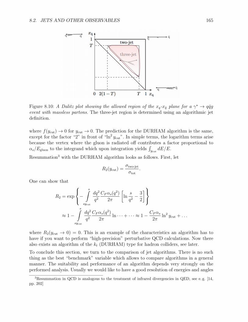
Now is a good time to recall the Dalitz plot of Fig. 8.4 where we separated a two-jet and athree-jet region. The algorithmic jet definition we have developed enables us to define thethee-jet region: Apply the jet algorithm until three jets are left. If the distance betweenthe jets can be resolved, min(i,j)(yij) > ycut, there are three jets, else it is a two-jet event.The shape of the found three-jet region is somewhat different, since yij also depends onthe angle θij, see Fig. 8.10.
In order to compare the analyzed data to the predictions of QCD, we need perturbativepredictions for jet rates. For the reaction e+e− → hadrons the leading order predictionsare as follows. For the JADE algorithm we have
σLOthree-jet(ycut) = σ0CFαs
2π
�
2 ln2 ycut + 3 ln ycut −π2
3+5
2− f(ycut)
�
(8.10)
8.2. JETS AND OTHER OBSERVABLES 165
Figure 8.10: A Dalitz plot showing the allowed region of the xq-xq̄ plane for a γ� → qq̄gevent with massless partons. The three-jet region is determined using an algorithmic jetdefinition.
where f(ycut)→ 0 for ycut → 0. The prediction for the DURHAM algorithm is the same,except for the factor “2” in front of “ln2 ycut”. In simple terms, the logarithm terms arisebecause the vertex where the gluon is radiated off contributes a factor proportional toαs/Egluon to the integrand which upon integration yields
�ycut
dE/E.
Resummation3 with the DURHAM algorithm looks as follows. First, let
R2(ycut) =σtwo-jetσtot
.
One can show that
R2 = exp
−
s�
sycut
dq2
q2CFαs(q
2)
2π
�
lns
q2−3
2
�
≈ 1−
s�
sycut
dq2
q2CFαs(q
2)
2πln · · ·+ · · · ≈ 1−
CFαs
2πln2 ycut + . . .
where R2(ycut → 0) = 0. This is an example of the characteristics an algorithm has tohave if you want to perform “high-precision” perturbative QCD calculations. Now therealso exists an algorithm of the kt (DURHAM) type for hadron colliders, see later.
To conclude this section, we turn to the comparison of jet algorithms. There is no suchthing as the best “benchmark” variable which allows to compare algorithms in a generalmanner. The suitability and performance of an algorithm depends very strongly on theperformed analysis. Usually we would like to have a good resolution of energies and angles
3Resummation in QCD is analogous to the treatment of infrared divergencies in QED, see e. g. [14,pp. 202]

166 CHAPTER 8. QCD IN E+E− ANNIHILATIONS
(a) (b)
Figure 8.11: Visualization of levels at which the algorithms have to deliver good resolution(a) and comparison of jet algorithms (b). The mean number of jets is displayed as afunction of ycut. The parton level is denoted by squares and the hadron level by circles.The results were obtained by HERWIG Monte Carlo simulation at ECM = Mz. Source:[34, p. 28]. For details compare [34, pp. 7].
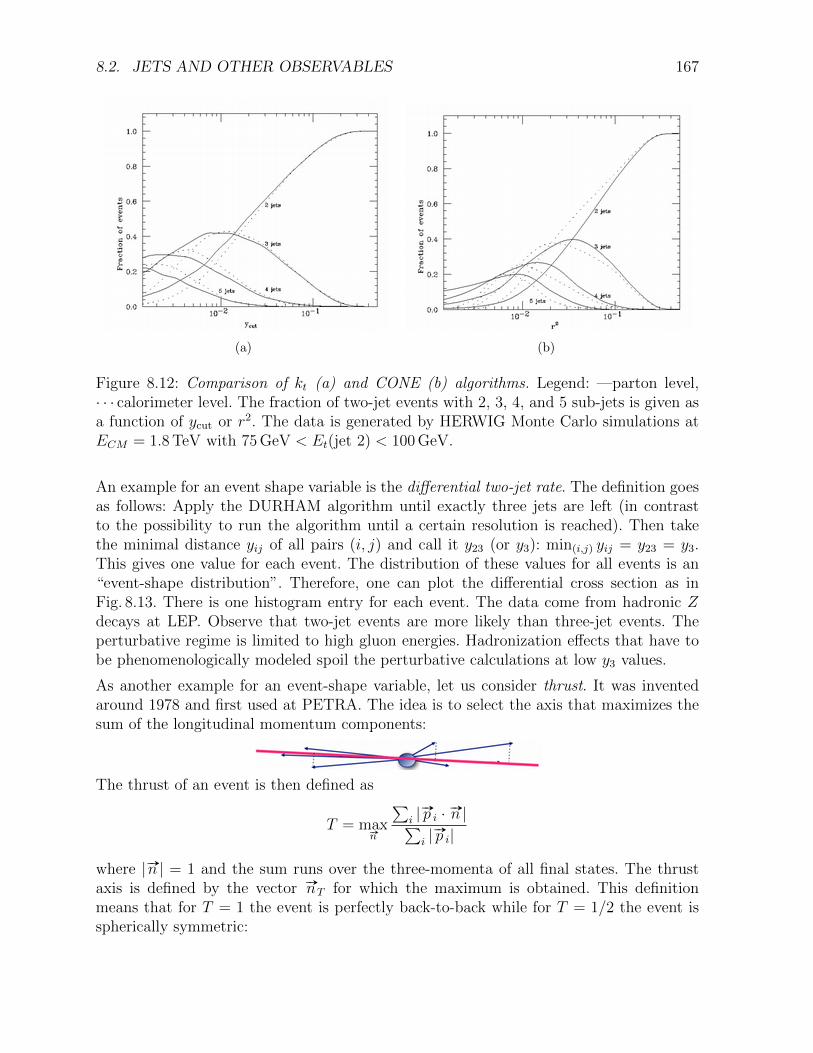
of the jets at the parton, hadron, and detector levels (see Fig. 8.11(a) for a visualization),as well as a good efficiency and purity to find a certain number of jets at a certainlevel. For some jet algorithms, the mean number of jets as a function of ycut at thehadron and parton levels, as obtained by HERWIG (Hadron Emission Reactions WithInterfering Gluons) Monte Carlo simulation at ECM = MZ , is compared in Fig. 8.11(b).Another comparison4 is shown in Fig. 8.12. The fraction of events with 2 jets which have2, 3, 4, and 5 sub-jets is given as a function of ycut or r2, the radius fraction sqared,respectively. The data stem from HERWIG Monte Carlo simulations at ECM = 1.8TeVwith 75GeV < Et(jet 2) < 100GeV. Data from a kt algorithm are shown in Fig. 8.12(a)while the results in Fig. 8.12(b) come from a CONE algorithm with radius R = 0.7.
8.2.2 Event shape variables
The introduced jet algorithms can be used as a starting point to define more refinedobservables that capture the event topologies.
4More on kt and CONE algorithms can be found in [41].
8.2. JETS AND OTHER OBSERVABLES 167
(a) (b)
Figure 8.12: Comparison of kt (a) and CONE (b) algorithms. Legend: —parton level,· · · calorimeter level. The fraction of two-jet events with 2, 3, 4, and 5 sub-jets is given asa function of ycut or r2. The data is generated by HERWIG Monte Carlo simulations atECM = 1.8TeV with 75GeV < Et(jet 2) < 100GeV.
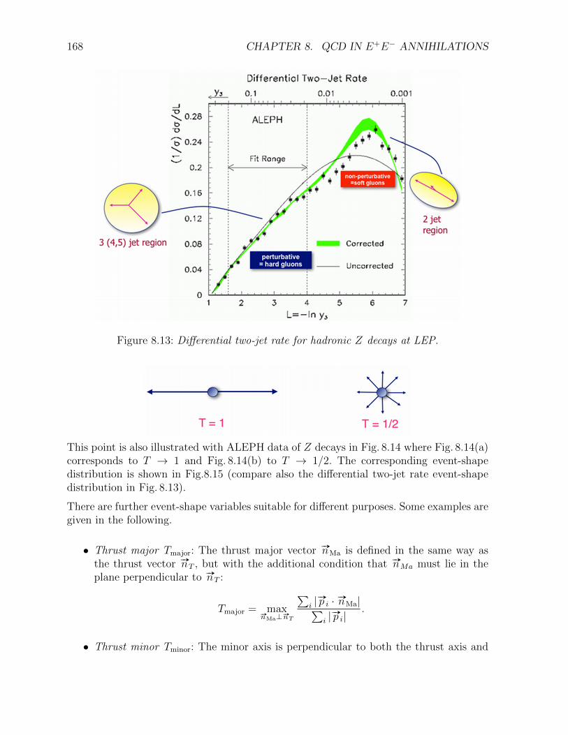
An example for an event shape variable is the differential two-jet rate. The definition goesas follows: Apply the DURHAM algorithm until exactly three jets are left (in contrastto the possibility to run the algorithm until a certain resolution is reached). Then takethe minimal distance yij of all pairs (i, j) and call it y23 (or y3): min(i,j) yij = y23 = y3.This gives one value for each event. The distribution of these values for all events is an“event-shape distribution”. Therefore, one can plot the differential cross section as inFig. 8.13. There is one histogram entry for each event. The data come from hadronic Zdecays at LEP. Observe that two-jet events are more likely than three-jet events. Theperturbative regime is limited to high gluon energies. Hadronization effects that have tobe phenomenologically modeled spoil the perturbative calculations at low y3 values.
As another example for an event-shape variable, let us consider thrust. It was inventedaround 1978 and first used at PETRA. The idea is to select the axis that maximizes thesum of the longitudinal momentum components:
The thrust of an event is then defined as
T = max#»n
�i |
#»p i ·#»n |
�i |
#»p i|
where | #»n | = 1 and the sum runs over the three-momenta of all final states. The thrustaxis is defined by the vector #»nT for which the maximum is obtained. This definitionmeans that for T = 1 the event is perfectly back-to-back while for T = 1/2 the event isspherically symmetric:
168 CHAPTER 8. QCD IN E+E− ANNIHILATIONS
Figure 8.13: Differential two-jet rate for hadronic Z decays at LEP.
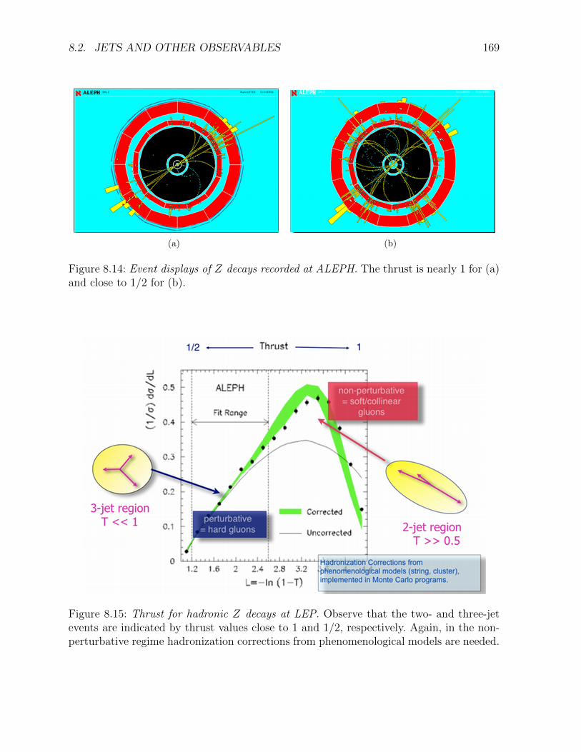
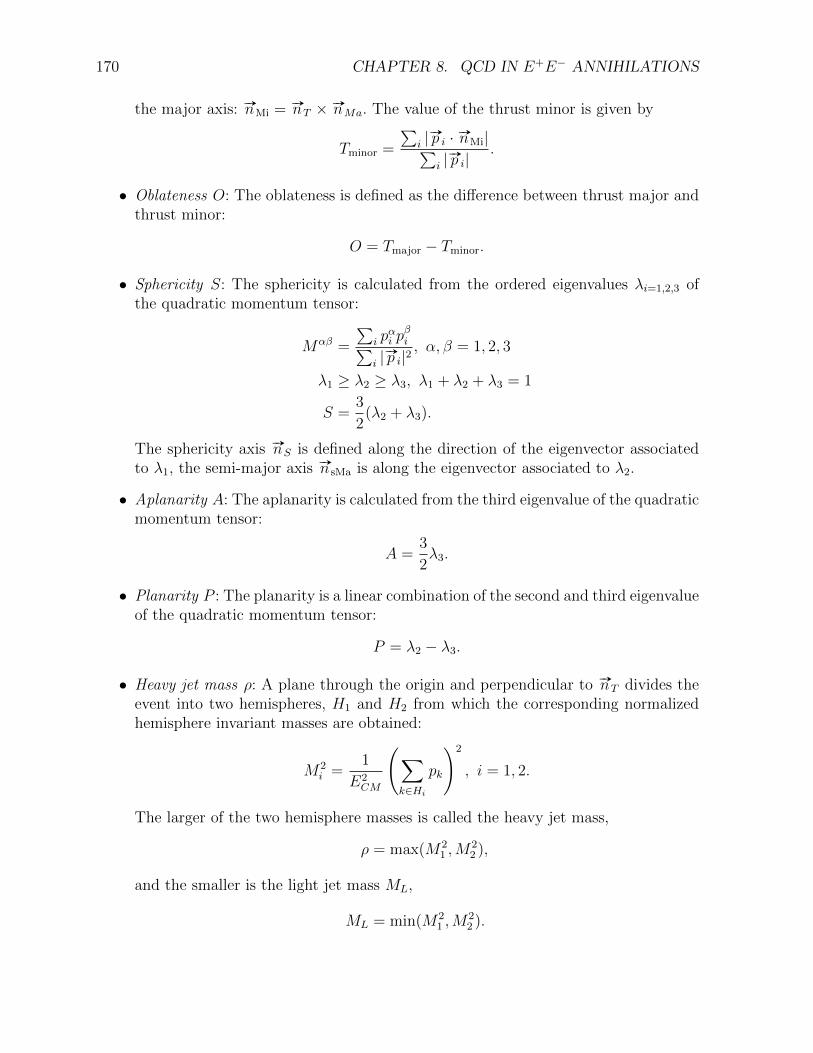
This point is also illustrated with ALEPH data of Z decays in Fig. 8.14 where Fig. 8.14(a)corresponds to T → 1 and Fig. 8.14(b) to T → 1/2. The corresponding event-shapedistribution is shown in Fig.8.15 (compare also the differential two-jet rate event-shapedistribution in Fig. 8.13).
There are further event-shape variables suitable for different purposes. Some examples aregiven in the following.
• Thrust major Tmajor: The thrust major vector#»nMa is defined in the same way as
the thrust vector #»nT , but with the additional condition that#»nMa must lie in the
plane perpendicular to #»nT :
Tmajor = max#»nMa⊥
#»nT
�i |
#»p i ·#»nMa|�
i |#»p i|
.
• Thrust minor Tminor: The minor axis is perpendicular to both the thrust axis and
8.2. JETS AND OTHER OBSERVABLES 169
(a) (b)
Figure 8.14: Event displays of Z decays recorded at ALEPH. The thrust is nearly 1 for (a)and close to 1/2 for (b).
Figure 8.15: Thrust for hadronic Z decays at LEP. Observe that the two- and three-jetevents are indicated by thrust values close to 1 and 1/2, respectively. Again, in the non-perturbative regime hadronization corrections from phenomenological models are needed.
170 CHAPTER 8. QCD IN E+E− ANNIHILATIONS
the major axis: #»nMi =#»nT × #»nMa. The value of the thrust minor is given by
Tminor =
�i |
#»p i ·#»nMi|�
i |#»p i|
.
• Oblateness O: The oblateness is defined as the difference between thrust major andthrust minor:
O = Tmajor − Tminor.
• Sphericity S: The sphericity is calculated from the ordered eigenvalues λi=1,2,3 ofthe quadratic momentum tensor:
Mαβ =
�i p
αi p
βi�
i |#»p i|2
, α, β = 1, 2, 3
λ1 ≥ λ2 ≥ λ3, λ1 + λ2 + λ3 = 1
S =3
2(λ2 + λ3).
The sphericity axis #»nS is defined along the direction of the eigenvector associatedto λ1, the semi-major axis
#»n sMa is along the eigenvector associated to λ2.
• Aplanarity A: The aplanarity is calculated from the third eigenvalue of the quadraticmomentum tensor:
A =3
2λ3.
• Planarity P : The planarity is a linear combination of the second and third eigenvalueof the quadratic momentum tensor:
P = λ2 − λ3.
• Heavy jet mass ρ: A plane through the origin and perpendicular to #»nT divides theevent into two hemispheres, H1 and H2 from which the corresponding normalizedhemisphere invariant masses are obtained:
M2i =
1
E2CM
��
k∈Hi
pk
�2
, i = 1, 2.
The larger of the two hemisphere masses is called the heavy jet mass,
ρ = max(M21 ,M
22 ),
and the smaller is the light jet mass ML,
ML = min(M21 ,M
22 ).
8.2. JETS AND OTHER OBSERVABLES 171
• Jet mass difference MD: The difference between ρ and ML is called the jet massdifference:
MD = ρ−ML.
• Wide jet broadening BW : A measure of the broadening of particles in transversemomentum with respect to the thrust axis can be calculated for each hemisphereHi using the relation
Bi =
�k∈Hi
| #»p k ×#»nT |
2�
j |#»p j|
, i = 1, 2
where j runs over all particles in the event. The wide jet broadening is the larger ofthe two hemisphere broadenings,
BW = max(B1, B2),
and the smaller is called the narrow jet broadening BN ,
BN = min(B1, B2).
• Total jet broadening BT : The total jet broadening is the sum of the wide and thenarrow jet broadenings:
BT = BW + BN .
• C-parameter C: The C-parameter is derived from the eigenvalues of the linearizedmomentum tensor Θαβ:
Θαβ =1
�i |
#»p i|
�
i
pαi pβi
| #»p i|, α, β = 1, 2, 3.
The eigenvalues λj of this tensor define C by
C = 3(λ1λ2 + λ2λ3 + λ3λ1).
The discussed event-shape variables have been extensively used to analyze LEP data.Examples are given in Fig. 8.16: Fig. 8.16(a) shows thrust predictions and measurements;predictions and data for thrust, heavy jet mass, total jet broadening, wide jet broadening,and the C-parameter are shown in Fig. 8.16(b).

172 CHAPTER 8. QCD IN E+E− ANNIHILATIONS
(a) (b)
Figure 8.16: Comparison of predictions and LEP data for some event-shape variables.Thrust data are shown for several center of mass energies (a). The other analyses dealwith heavy jet mass, total jet broadening, wide jet broadening, and the C-parameter (b).
8.2.3 Applications
Examples for applications of the observables discussed above in this section are measure-ments of the strong coupling constant αs (see later, Sect. 8.3), the discovery of quark andgluon jets, measurements of the quark and gluon spin, the triple-gluon vertex, and jetrates or the analysis of differences between quark and gluon jets.
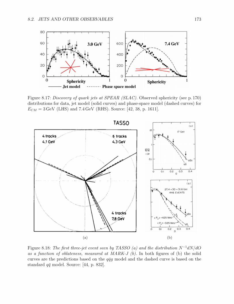
Quark jets were discovered at the SPEAR storage ring (SLAC) [42]. The data are shownin Fig. 8.17. For higher energies particles cluster around an axis and the Monte Carlosimulation based on a jet model fits the data better than the simulation based on anisotropic phase-space model. This is the first observation of a jet structure.
Gluon jets were discovered at PETRA (DESY) [43, 44, 45, 46]. Here, the relevant ob-servable is oblateness (see p. 170). The first three-jet event seen by TASSO is shown inFig. 8.18(a). In Fig. 8.18(b) one can observe that events at ECM ∼ 30GeV exhibit largeroblateness (planar structure) than predicted by models without hard gluon radiation.
When it comes to parton spins the question is: How do you measure the spin of unob-servable particles? For spin-1/2 fermions annihilating into a vector boson, conservation ofangular momentum predicts a distribution
dσ
d cosΘ∗∼ 1 + cos2Θ∗
8.2. JETS AND OTHER OBSERVABLES 173
Figure 8.17: Discovery of quark jets at SPEAR (SLAC). Observed sphericity (see p. 170)distributions for data, jet model (solid curves) and phase-space model (dashed curves) forECM = 3GeV (LHS) and 7.4GeV (RHS). Source: [42, 38, p. 1611].
(a) (b)
Figure 8.18: The first three-jet event seen by TASSO (a) and the distribution N−1dN/dOas a function of oblateness, measured at MARK-J (b). In both figures of (b) the solidcurves are the predictions based on the qq̄g model and the dashed curve is based on thestandard qq̄ model. Source: [44, p. 832].
174 CHAPTER 8. QCD IN E+E− ANNIHILATIONS
(a) (b)
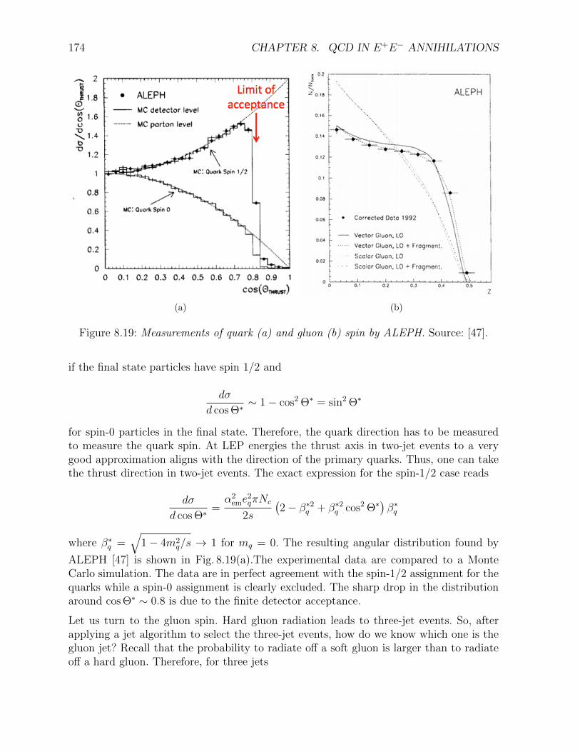
Figure 8.19: Measurements of quark (a) and gluon (b) spin by ALEPH. Source: [47].
if the final state particles have spin 1/2 and
dσ
d cosΘ∗∼ 1− cos2Θ∗ = sin2Θ∗
for spin-0 particles in the final state. Therefore, the quark direction has to be measuredto measure the quark spin. At LEP energies the thrust axis in two-jet events to a verygood approximation aligns with the direction of the primary quarks. Thus, one can takethe thrust direction in two-jet events. The exact expression for the spin-1/2 case reads
dσ
d cosΘ∗=
α2eme2qπNc
2s
�2− β∗2
q + β∗2q cos2Θ∗
�β∗q
where β∗q =
�1− 4m2q/s → 1 for mq = 0. The resulting angular distribution found by
ALEPH [47] is shown in Fig. 8.19(a).The experimental data are compared to a MonteCarlo simulation. The data are in perfect agreement with the spin-1/2 assignment for thequarks while a spin-0 assignment is clearly excluded. The sharp drop in the distributionaround cosΘ∗ ∼ 0.8 is due to the finite detector acceptance.
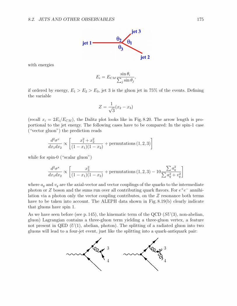
Let us turn to the gluon spin. Hard gluon radiation leads to three-jet events. So, afterapplying a jet algorithm to select the three-jet events, how do we know which one is thegluon jet? Recall that the probability to radiate off a soft gluon is larger than to radiateoff a hard gluon. Therefore, for three jets
8.2. JETS AND OTHER OBSERVABLES 175
with energies
Ei = ECMsin θi�j sin θj
,
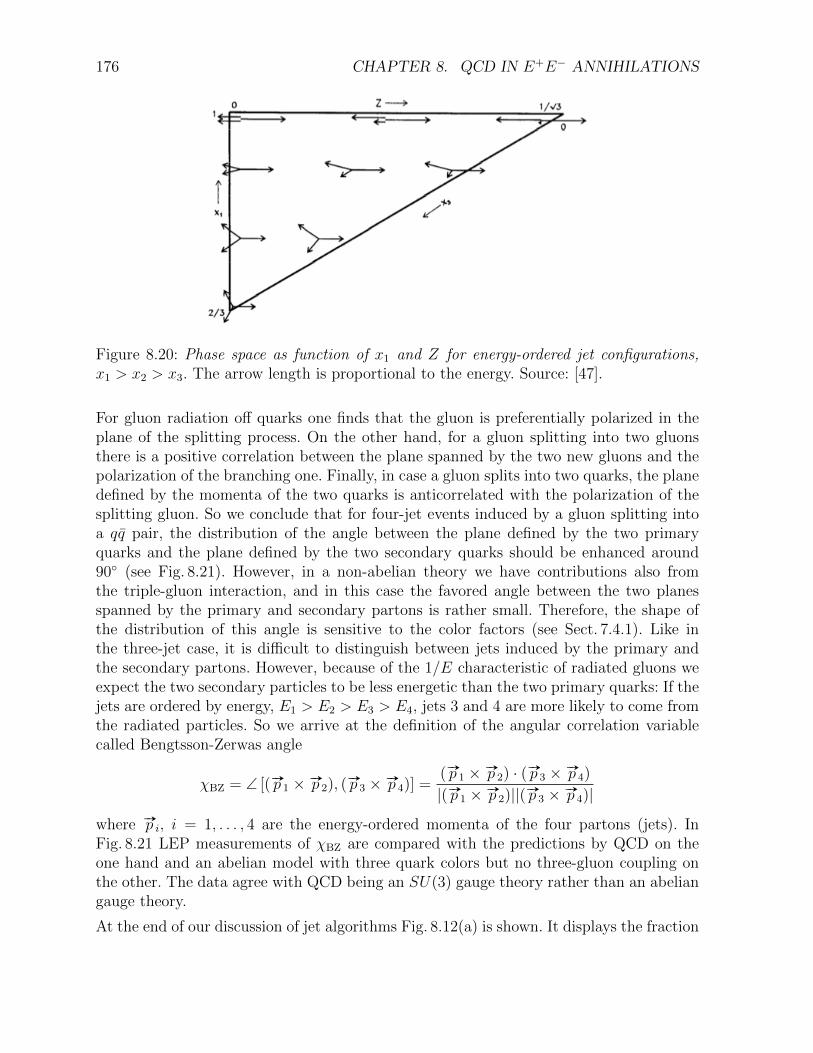
if ordered by energy, E1 > E2 > E3, jet 3 is the gluon jet in 75% of the events. Definingthe variable
Z =1√3(x2 − x3)
(recall xi = 2Ei/ECM), the Dalitz plot looks like in Fig. 8.20. The arrow length is pro-portional to the jet energy. The following cases have to be compared: In the spin-1 case(“vector gluon”) the prediction reads
d2σv
dx1dx2∝
�x21 + x22
(1− x1)(1− x2)+ permutations (1, 2, 3)
�
while for spin-0 (“scalar gluon”)
d2σs
dx1dx2∝
�x23
(1− x1)(1− x2)+ permutations (1, 2, 3)− 10
�a2q�
a2q + v2q
�
where aq and vq are the axial-vector and vector couplings of the quarks to the intermediatephoton or Z boson and the sums run over all contributing quark flavors. For e+e− annihi-lation via a photon only the vector coupling contributes, on the Z resonance both termshave to be taken into account. The ALEPH data shown in Fig. 8.19(b) clearly indicatethat gluons have spin 1.
As we have seen before (see p. 145), the kinematic term of the QCD (SU(3), non-abelian,gluon) Lagrangian contains a three-gluon term yielding a three-gluon vertex, a featurenot present in QED (U(1), abelian, photon). The splitting of a radiated gluon into twogluons will lead to a four-jet event, just like the splitting into a quark-antiquark pair:
� 4
3
� 4
3
176 CHAPTER 8. QCD IN E+E− ANNIHILATIONS
Figure 8.20: Phase space as function of x1 and Z for energy-ordered jet configurations,x1 > x2 > x3. The arrow length is proportional to the energy. Source: [47].
For gluon radiation off quarks one finds that the gluon is preferentially polarized in theplane of the splitting process. On the other hand, for a gluon splitting into two gluonsthere is a positive correlation between the plane spanned by the two new gluons and thepolarization of the branching one. Finally, in case a gluon splits into two quarks, the planedefined by the momenta of the two quarks is anticorrelated with the polarization of thesplitting gluon. So we conclude that for four-jet events induced by a gluon splitting intoa qq̄ pair, the distribution of the angle between the plane defined by the two primaryquarks and the plane defined by the two secondary quarks should be enhanced around90◦ (see Fig. 8.21). However, in a non-abelian theory we have contributions also fromthe triple-gluon interaction, and in this case the favored angle between the two planesspanned by the primary and secondary partons is rather small. Therefore, the shape ofthe distribution of this angle is sensitive to the color factors (see Sect. 7.4.1). Like inthe three-jet case, it is difficult to distinguish between jets induced by the primary andthe secondary partons. However, because of the 1/E characteristic of radiated gluons weexpect the two secondary particles to be less energetic than the two primary quarks: If thejets are ordered by energy, E1 > E2 > E3 > E4, jets 3 and 4 are more likely to come fromthe radiated particles. So we arrive at the definition of the angular correlation variablecalled Bengtsson-Zerwas angle
χBZ = ∠ [( #»p 1 ×#»p 2), (
#»p 3 ×#»p 4)] =
( #»p 1 ×#»p 2) · (
#»p 3 ×#»p 4)
|( #»p 1 ×#»p 2)||(
#»p 3 ×#»p 4)|
where #»p i, i = 1, . . . , 4 are the energy-ordered momenta of the four partons (jets). InFig. 8.21 LEP measurements of χBZ are compared with the predictions by QCD on theone hand and an abelian model with three quark colors but no three-gluon coupling onthe other. The data agree with QCD being an SU(3) gauge theory rather than an abeliangauge theory.
At the end of our discussion of jet algorithms Fig. 8.12(a) is shown. It displays the fraction

8.2. JETS AND OTHER OBSERVABLES 177
Figure 8.21: Distribution of χBZ measured by L3. The predictions for QCD and the abelianmodel are shown as bands indicating the theoretical uncertainties. Source: [48, p. 233].
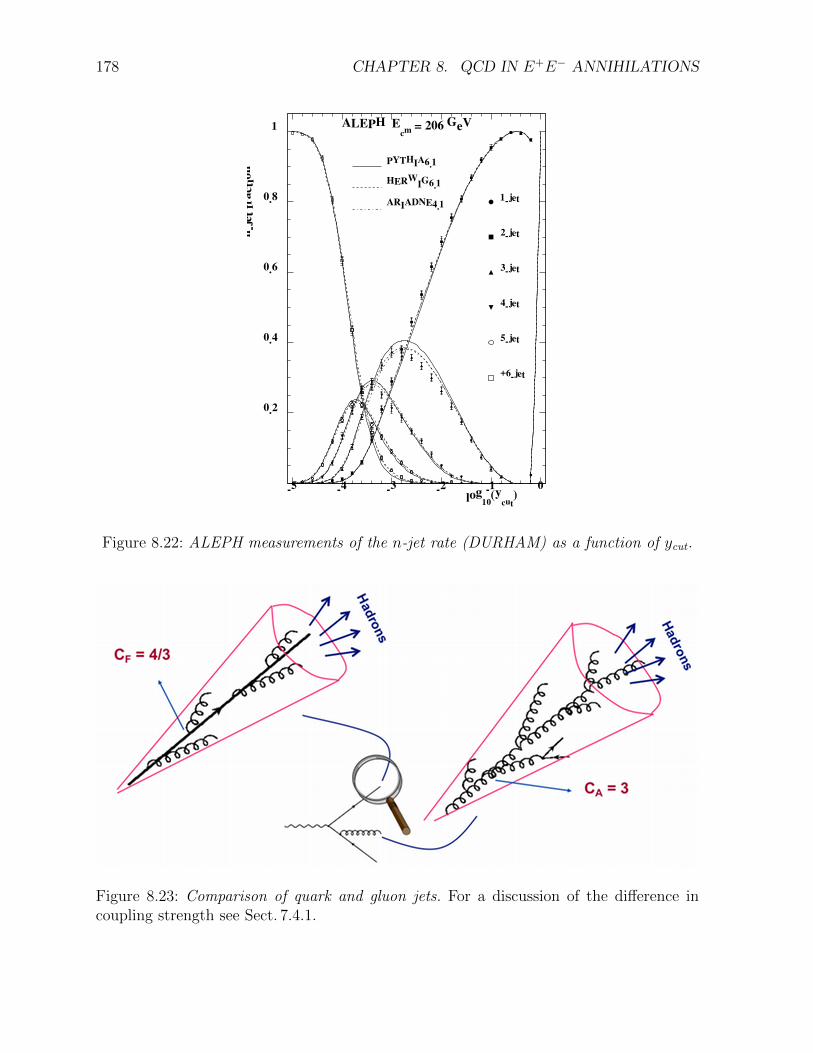
of 2-jet events with 2, 3, 4, and 5 sub-jets as a function of ycut. These predictions canbe tested comparing measurements at highest LEP energies to Monte Carlo simulationswhich incorporate leading-order matrix elements for two-jet and three-jet production, plusapproximations for multiple soft or collinear gluon radiation. Fig. 8.22 shows the n-jet rateaccording to the DURHAM (kt) algorithm as a function of ycut.
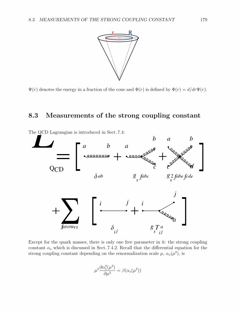
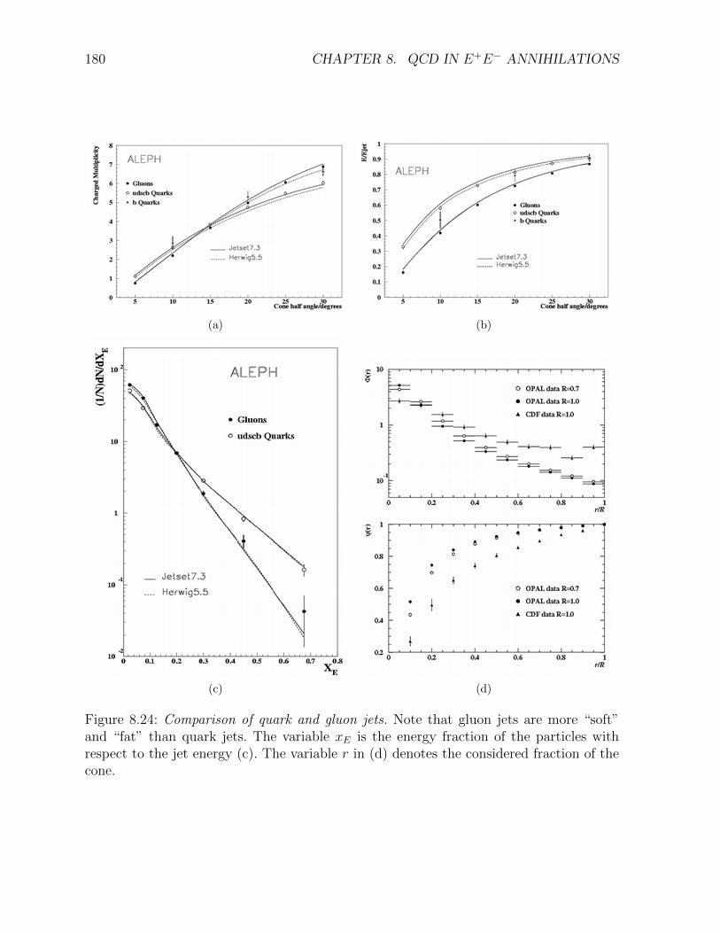
We conclude this section with a discussion of the differences between quark and gluon jets.Quark and gluon jets have different coupling strengths to emit gluons (see Sect. 7.4.1 andFig. 8.23). Therefore, from couplings alone one expects a larger multiplicity in gluon jetsof the order CA/CF = 9/4, and a softening of the momentum distributions for particlescoming from the gluon jet. Thus gluon jets are more “soft” and “fat” than quark jets(see Fig. 8.24). Also the scaling violations, i. e. change of multiplicities with energy andmomentum scale are different. In Fig. 8.24(d) the CONE algorithm is applied to dataof OPAL (LEP) and compared to CDF data. The variable r denotes the radius of theconsidered cone fraction when R is the radius parameter of the cone algorithm:
178 CHAPTER 8. QCD IN E+E− ANNIHILATIONSS =2(λ + λ ) .
n-j
et f
ract
ion
ALEPH Ecm
= 206 GeV
PYTHIA6.1
HERWIG6.1
ARIADNE4.11-jet
2-jet
3-jet
4-jet
5-jet
+6-jet
log10
(ycut
)
0.2
0.4
0.6
0.8
1
-5 -4 -3 -2 -1 0
Figure 8.22: ALEPH measurements of the n-jet rate (DURHAM) as a function of ycut.
Figure 8.23: Comparison of quark and gluon jets. For a discussion of the difference incoupling strength see Sect. 7.4.1.
8.3. MEASUREMENTS OF THE STRONG COUPLING CONSTANT 179
Ψ(r) denotes the energy in a fraction of the cone and Φ(r) is defined by Φ(r) = d/drΨ(r).
8.3 Measurements of the strong coupling constant
The QCD Lagrangian is introduced in Sect. 7.4:
LQCD
�ab
�ij
gs f abc
gsTija
gs2f abef cde
a
i ij
j
a
ab
b
c c d
ba
flavours
Except for the quark masses, there is only one free parameter in it: the strong couplingconstant αs which is discussed in Sect. 7.4.2. Recall that the differential equation for thestrong coupling constant depending on the renormalization scale µ, αs(µ
2), is
µ2∂α2s(µ
2)
∂µ2= β(αs(µ
2))
180 CHAPTER 8. QCD IN E+E− ANNIHILATIONS
(a) (b)
(c) (d)
Figure 8.24: Comparison of quark and gluon jets. Note that gluon jets are more “soft”and “fat” than quark jets. The variable xE is the energy fraction of the particles withrespect to the jet energy (c). The variable r in (d) denotes the considered fraction of thecone.
8.3. MEASUREMENTS OF THE STRONG COUPLING CONSTANT 181
which, retaining only the first term of the power expansion for β and absorbing the factorof 4π into the coefficient β0, yields
αs(Q2) ≡
g2s(Q2)
4π=
1
β0 ln(Q2/Λ2QCD).
At that point we also stressed that
β0 =1
4π
�
11−2
3nf
�
> 0 for (the likely case of) nf < 17
which makes the effective coupling constant behave like shown in Fig. 7.4.2. The followingexpansion holds for αs(µ
2) (see Eq. (7.43)):
αs(µ2) ≈ αs(Q
2)
�
1− αs(Q2)β0 ln
µ2
Q2+ α2s(Q
2)β20 ln2 µ2
Q2+O(α3s)
�
. (8.11)
To measure the coupling strength one uses as many methods as possible in order todemonstrate that QCD really is the correct theory of strong interactions by showing thatone universal coupling constant describes all strong interactions phenomena. Consider theperturbative expansion of the cross section for some QCD process:
σpert = αs(µ2)A+ α2s(µ
2)
�
B + β0A lnµ2
Q2
�
+O(α3s) (8.12)
where the coefficients A and B depend on the specific process. So, if only the leading oder(LO) expansion is known, the following holds:
σpertLO = αs(µ2)A = αs(Q
2)A− α2s(Q2)β0A ln
µ2
Q2+O(α2s)
where in the second step we inserted the expansion from Eq. (8.11). This means that theresult depends strongly on the choice of the renormalization scale µ. Since the correctionsto the cross section can be relatively large, it is possible to find significantly differentvalues for the measured effective coupling constant αmeas,effs for two different processes:Consider two processes, where the LO calculations predict
σpertLO;1 = αsA1
σpertLO;2 = αsA2.
The predictions are compared to the cross sections σexp1 and σexp2 from experiment. Finally,because of the said strong scale dependence, the result may be αmeas,effs;1 �= αmeas,effs;1 .
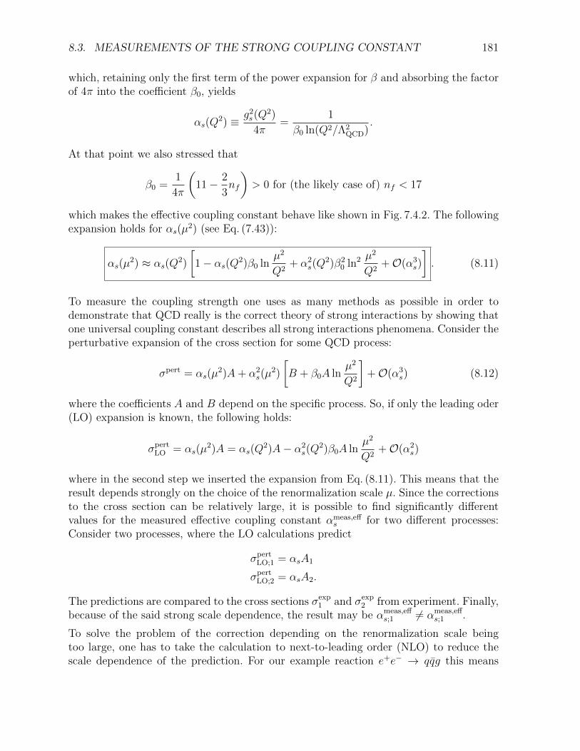
To solve the problem of the correction depending on the renormalization scale beingtoo large, one has to take the calculation to next-to-leading order (NLO) to reduce thescale dependence of the prediction. For our example reaction e+e− → qq̄g this means
182 CHAPTER 8. QCD IN E+E− ANNIHILATIONS
�e+
e−
q̄
g
q
�e+
e−
q̄
g
g
q
�e+
e−
q̄
g
q
�e+
e−
q̄
g
q
Figure 8.25: Feynman diagrams for e+e− → qq̄g to NLO.
considering the diagrams shown in Fig. 8.25. The NLO expression is again obtained fromthe expansion in Eq. (8.12):
σpertNLO = αs(µ2)A+ α2s(µ
2)
�
B + β0A lnµ2
Q2
�
+O(α3s)
= αs(Q2)A+ α2s(Q
2)B + α3s(Q2)β20A
2 ln2µ2
Q2+O(α4s)
where in the second line we inserted for αs(µ2) the expansion from Eq. (8.11) and the
dependence on ln(µ2/Q2) cancels. Thus, the scale dependence of the prediction is muchsmaller than in the LO case. The scale dependence cancels completely at fully calculatedorder.
By comparing the NLO prediction for the cross section to experiment, one can extractαs(Q
2), e. g. αs(M2Z). This information can in turn be used to predict other process cross
sections at NLO. Furthermore, by varying the scale µ2 one can estimate the size of theNNLO contributions.
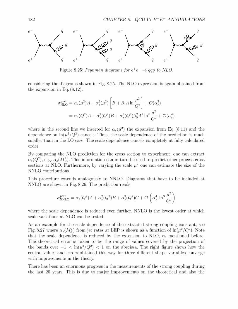
This procedure extends analogously to NNLO. Diagrams that have to be included atNNLO are shown in Fig. 8.26. The prediction reads
σpertNNLO = αs(Q2)A+ α2s(Q
2)B + α3s(Q2)C +O
�
α4s, ln3 µ2
Q2
�
where the scale dependence is reduced even further. NNLO is the lowest order at whichscale variations at NLO can be tested.
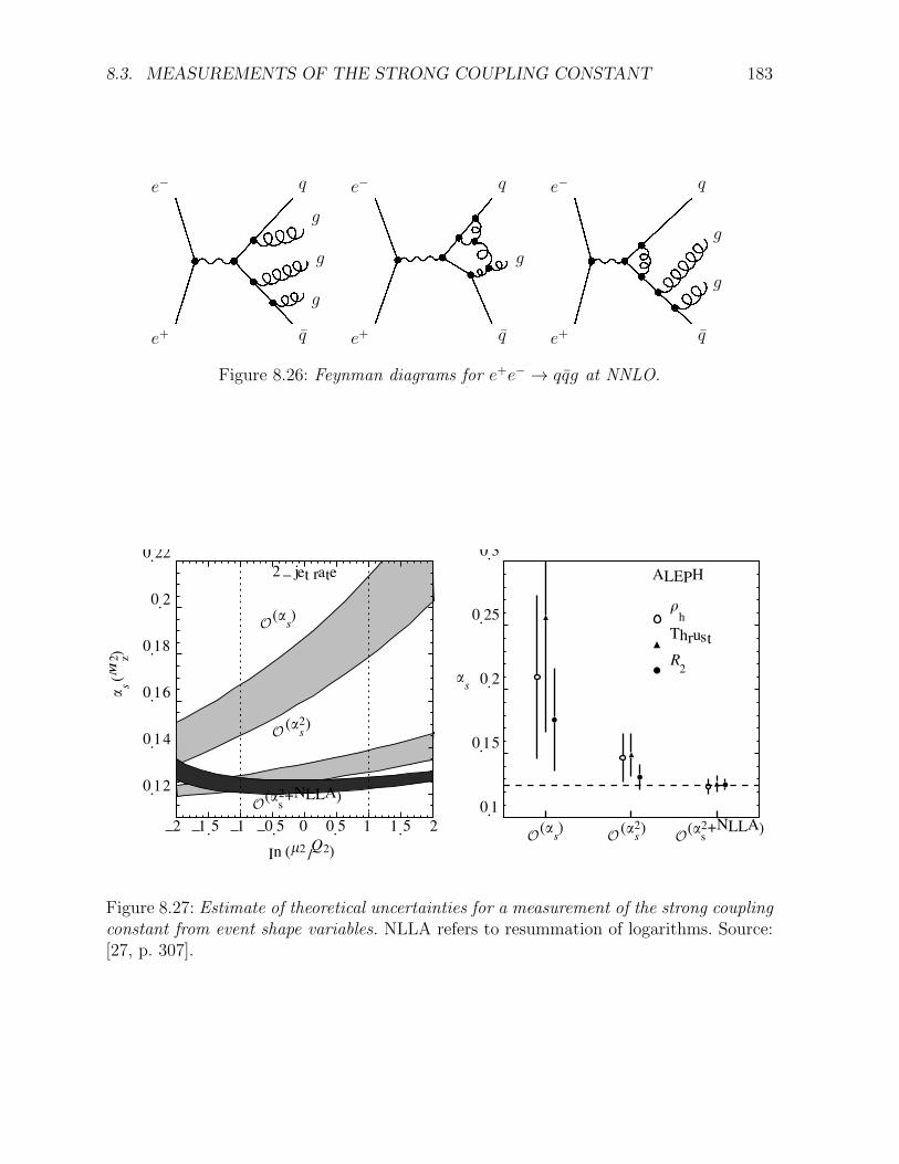
As an example for the scale dependence of the extracted strong coupling constant, seeFig. 8.27 where αs(M
2Z) from jet rates at LEP is shown as a function of ln(µ2/Q2). Note
that the scale dependence is reduced by the extension to NLO, as mentioned before.The theoretical error is taken to be the range of values covered by the projection ofthe bands over −1 < ln(µ2/Q2) < 1 on the abscissa. The right figure shows how thecentral values and errors obtained this way for three different shape variables convergewith improvements in the theory.
There has been an enormous progress in the measurements of the strong coupling duringthe last 20 years. This is due to major improvements on the theoretical and also the
8.3. MEASUREMENTS OF THE STRONG COUPLING CONSTANT 183
�e+
e−
q̄
g
g
g
q
�e+
e−
q̄
g
q
�e+
e−
q̄
g
g
q
Figure 8.26: Feynman diagrams for e+e− → qq̄g at NNLO.
constructed such that it is reasonable to interpret them like conventional 68%confidence level intervals.
2 – jet rate
(�s)
(�2s)
�s
(M2 z)
(�2s +NLLA)
In (�2/Q2)
0.12
0.14
0.16
0.18
0.2
0.22
–2 –1.5 –1 –0.5 0 0.5 1 1.5 2
�s
0.1
0.15
0.2
0.25
0.3
ALEPH
(�s)
(�2s)
(�2s +NLLA)
�h
R2
Thrust
Fig. 8.1. Estimate of theoretical uncertainties for a measurement of the strongFigure 8.27: Estimate of theoretical uncertainties for a measurement of the strong couplingconstant from event shape variables. NLLA refers to resummation of logarithms. Source:[27, p. 307].
184 CHAPTER 8. QCD IN E+E− ANNIHILATIONS
��� ��������������������������� �
���
���
���
���
���
������
� �� ����������
���������������������������������
�������������������������
���������������
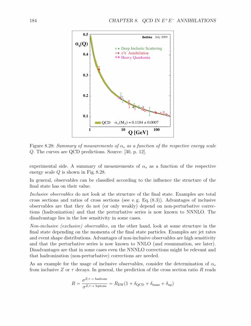
Figure 8.28: Summary of measurements of αs as a function of the respective energy scaleQ. The curves are QCD predictions. Source: [30, p. 12].
experimental side. A summary of measurements of αs as a function of the respectiveenergy scale Q is shown in Fig. 8.28.
In general, observables can be classified according to the influence the structure of thefinal state has on their value.
Inclusive observables do not look at the structure of the final state. Examples are totalcross sections and ratios of cross sections (see e. g. Eq. (8.3)). Advantages of inclusiveobservables are that they do not (or only weakly) depend on non-perturbative correc-tions (hadronization) and that the perturbative series is now known to NNNLO. Thedisadvantage lies in the low sensitivity in some cases.
Non-inclusive (exclusive) observables , on the other hand, look at some structure in thefinal state depending on the momenta of the final state particles. Examples are jet ratesand event shape distributions. Advantages of non-inclusive observables are high sensitivityand that the perturbative series is now known to NNLO (and resummation, see later).Disadvantages are that in some cases even the NNNLO corrections might be relevant andthat hadronization (non-perturbative) corrections are needed.
As an example for the usage of inclusive observables, consider the determination of αs
from inclusive Z or τ decays. In general, the prediction of the cross section ratio R reads
R =σZ,τ→ hadrons
σZ,τ→ leptons= REW(1 + δQCD + δmass + δnp)
8.3. MEASUREMENTS OF THE STRONG COUPLING CONSTANT 185
where the overall factor REW depends on the electroweak couplings of the quarks.5 Thecorrections are dominated by the perturbative QCD correction δQCD. The other termstake into account the finite quark masses and the non-perturbative corrections. The per-turbative QCD correction term is given by
δQCD = c1αs
π+ c2
�αs
π
�2+ c3
�αs
π
�3+ . . . .
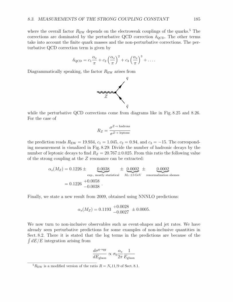
Diagrammatically speaking, the factor REW arises from
�Zq̄
q
while the perturbative QCD corrections come from diagrams like in Fig. 8.25 and 8.26.For the case of
RZ =σZ→ hadrons
σZ→ leptons
the prediction reads REW = 19.934, c1 = 1.045, c2 = 0.94, and c3 = −15. The correspond-ing measurement is visualized in Fig. 8.29: Divide the number of hadronic decays by thenumber of leptonic decays to find RZ = 20.767±0.025. From this ratio the following valueof the strong coupling at the Z resonance can be extracted:
αs(MZ) = 0.1226± 0.0038� �� �exp., mostly statistical
± 0.0002� �� �Mt:±5GeV
± 0.0002� �� �renormalization shemes
= 0.1226+0.0058−0.0038
.
Finally, we state a new result from 2009, obtained using NNNLO predictions:
αs(MZ) = 0.1193+0.0028−0.0027
± 0.0005.
We now turn to non-inclusive observables such as event-shapes and jet rates. We havealready seen perturbative predictions for some examples of non-inclusive quantities inSect. 8.2. There it is stated that the log terms in the predictions are because of the�dE/E integration arising from
dσq→qg
dEgluon∝ σ0
αs
2π
1
Egluon
5REW is a modified version of the ratio R = Nc11/9 of Sect. 8.1.
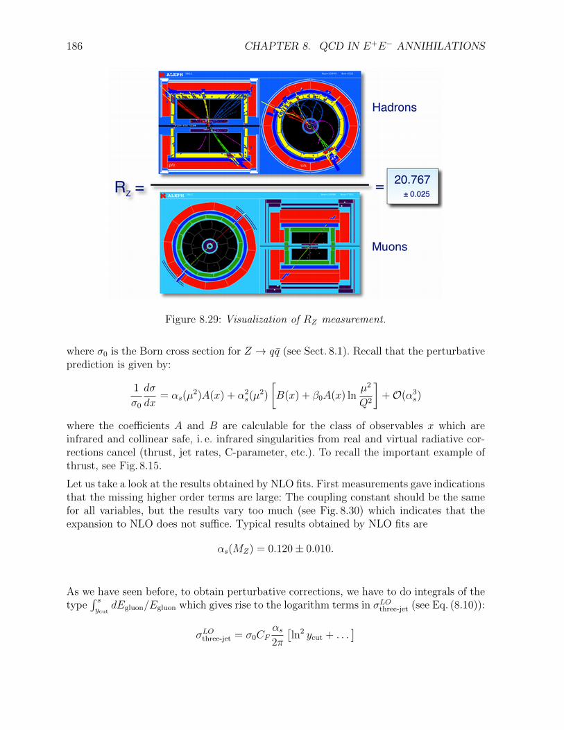
186 CHAPTER 8. QCD IN E+E− ANNIHILATIONS
Figure 8.29: Visualization of RZ measurement.
where σ0 is the Born cross section for Z → qq̄ (see Sect. 8.1). Recall that the perturbativeprediction is given by:
1
σ0
dσ
dx= αs(µ
2)A(x) + α2s(µ2)
�
B(x) + β0A(x) lnµ2
Q2
�
+O(α3s)
where the coefficients A and B are calculable for the class of observables x which areinfrared and collinear safe, i. e. infrared singularities from real and virtual radiative cor-rections cancel (thrust, jet rates, C-parameter, etc.). To recall the important example ofthrust, see Fig. 8.15.
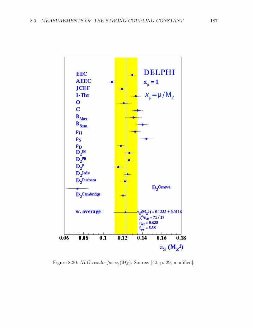
Let us take a look at the results obtained by NLO fits. First measurements gave indicationsthat the missing higher order terms are large: The coupling constant should be the samefor all variables, but the results vary too much (see Fig. 8.30) which indicates that theexpansion to NLO does not suffice. Typical results obtained by NLO fits are
αs(MZ) = 0.120± 0.010.
As we have seen before, to obtain perturbative corrections, we have to do integrals of thetype
� sycut
dEgluon/Egluon which gives rise to the logarithm terms in σLOthree-jet (see Eq. (8.10)):
σLOthree-jet = σ0CFαs
2π
�ln2 ycut + . . .
�
8.3. MEASUREMENTS OF THE STRONG COUPLING CONSTANT 187
�������
Figure 8.30: NLO results for αs(MZ). Source: [40, p. 29, modified].
188 CHAPTER 8. QCD IN E+E− ANNIHILATIONS
where the color factor CF = 4/3—the problem being that for ycut → 0 the series does notconverge.6 The resummation procedure mentioned earlier (see p. 165) also works for thethree-jet rate:
R3 =CFαs
2πln2 ycut −
C2Fα2s
8π2ln4 ycut + . . .
= 1− exp
−
s�
sycut
dq2
q2CFαs(q
2)
2π
�
lns
q2−3
2
�
.
Combined (to avoid double counting of logarithmic terms in resummed expressions andin full fixed order prediction) with full NLO calculations this gives theoretically muchimproved predictions. Typical results are:
αs(MZ) = 0.120± 0.005.
There are different sources of the remaining uncertainties. Experimental uncertaintiesinclude
• track reconstruction,
• event selection,
• detector corrections (via cut variations or different Monte Carlo generators),
• background subtraction (LEP2), and
• ISR corrections (LEP2).
They amount to about 1% uncertainty. Furthermore, there are hadronization uncertain-ties arising from the differences in behavior of various models for hadronization such asPYTHIA (string fragmentation), HERWIG (cluster fragmentation), or ARIADNE (dipolemodel and string fragmentation). Theses uncertainties are typically about 0.7 to 1.5%.Finally, there are also theoretical uncertainties, for instance
• renormalization scale variation,
• matching of NLO with resummed calculation, and
• quark mass effects.
6Recall that ycut is the resolution parameter deciding if two particles are distinguished or seen as onepseudo-particle.
8.3. MEASUREMENTS OF THE STRONG COUPLING CONSTANT 189
(a) (b)
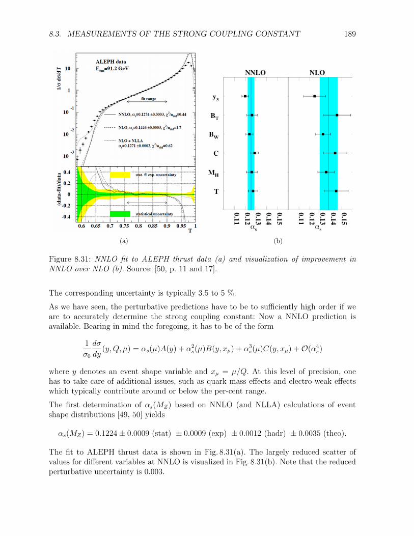
Figure 8.31: NNLO fit to ALEPH thrust data (a) and visualization of improvement inNNLO over NLO (b). Source: [50, p. 11 and 17].
The corresponding uncertainty is typically 3.5 to 5 %.
As we have seen, the perturbative predictions have to be to sufficiently high order if weare to accurately determine the strong coupling constant: Now a NNLO prediction isavailable. Bearing in mind the foregoing, it has to be of the form
1
σ0
dσ
dy(y,Q, µ) = αs(µ)A(y) + α2s(µ)B(y, xµ) + α3s(µ)C(y, xµ) +O(α4s)
where y denotes an event shape variable and xµ = µ/Q. At this level of precision, onehas to take care of additional issues, such as quark mass effects and electro-weak effectswhich typically contribute around or below the per-cent range.
The first determination of αs(MZ) based on NNLO (and NLLA) calculations of eventshape distributions [49, 50] yields
αs(MZ) = 0.1224± 0.0009 (stat) ± 0.0009 (exp) ± 0.0012 (hadr) ± 0.0035 (theo).
The fit to ALEPH thrust data is shown in Fig. 8.31(a). The largely reduced scatter ofvalues for different variables at NNLO is visualized in Fig. 8.31(b). Note that the reducedperturbative uncertainty is 0.003.
190 CHAPTER 8. QCD IN E+E− ANNIHILATIONS
The most precise determination of the strong coupling constant is obtained from jetobservables at LEP. Precision at the 2% level is achieved from the three-jet rate [51]:
αs(MZ) = 0.1175± 0.0020 (exp) ± 0.0015 (theo).
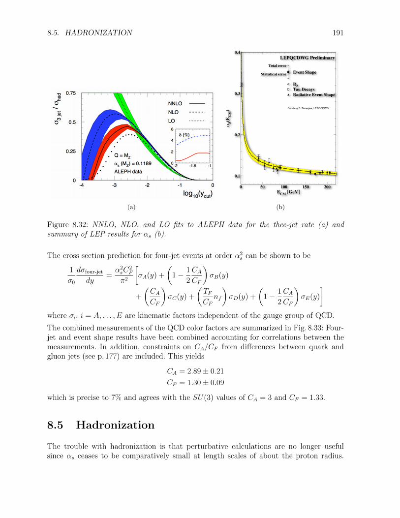
The three-jet rate is known to have small non-perturbative corrections and to be verystable under scale variations (for a certain range of the jet resolution parameter). For acomparison of LO, NLO, and NNLO predictions to the corresponding ALEPH data, seeFig. 8.32(a).
The LEP results concerning the determination of the strong coupling constant (seeFig.8.32(b)) can be summarized as follows (combination by S. Bethke, a couple of yearsago).
• Tau decays (NNLO)
αs(MZ) = 0.1181± 0.0030
• RZ (NNLO)
αs(MZ) = 0.1226+0.0058−0.0038
• Event shapes (NLO + NNLO)
αs(MZ) = 0.1202± 0.0050
• All (not including recent NNNLO results)
αs(MZ) = 0.1195± 0.0035
• Latest world average (S. Bethke, 2009 [30])
αs(MZ) = 0.1184± 0.0007
8.4 Measurements of the QCD color factors
Because they determine the gauge structure of strong interactions, the color factors arethe most important numbers in QCD, besides αs. Discussing the triple-gluon vertex weconcluded that our observables also allow to test the gauge structure of QCD. We havealready learned that the color factors (for SU(3)) CF = 4/3, CA = 3, and TF = 1/2measure the relative probabilities of gluon radiation (q → qg), triple gluon vertex (g →gg), and gluon splitting (g → qq̄).
8.5. HADRONIZATION 191
(a)
������������������������������
(b)
Figure 8.32: NNLO, NLO, and LO fits to ALEPH data for the thee-jet rate (a) andsummary of LEP results for αs (b).
The cross section prediction for four-jet events at order α2s can be shown to be
1
σ0
dσfour-jetdy
=α2sC
2F
π2
�
σA(y) +
�
1−1
2
CA
CF
�
σB(y)
+
�CA
CF
�
σC(y) +
�TFCF
nf
�
σD(y) +
�
1−1
2
CA
CF
�
σE(y)
�
where σi, i = A, . . . , E are kinematic factors independent of the gauge group of QCD.
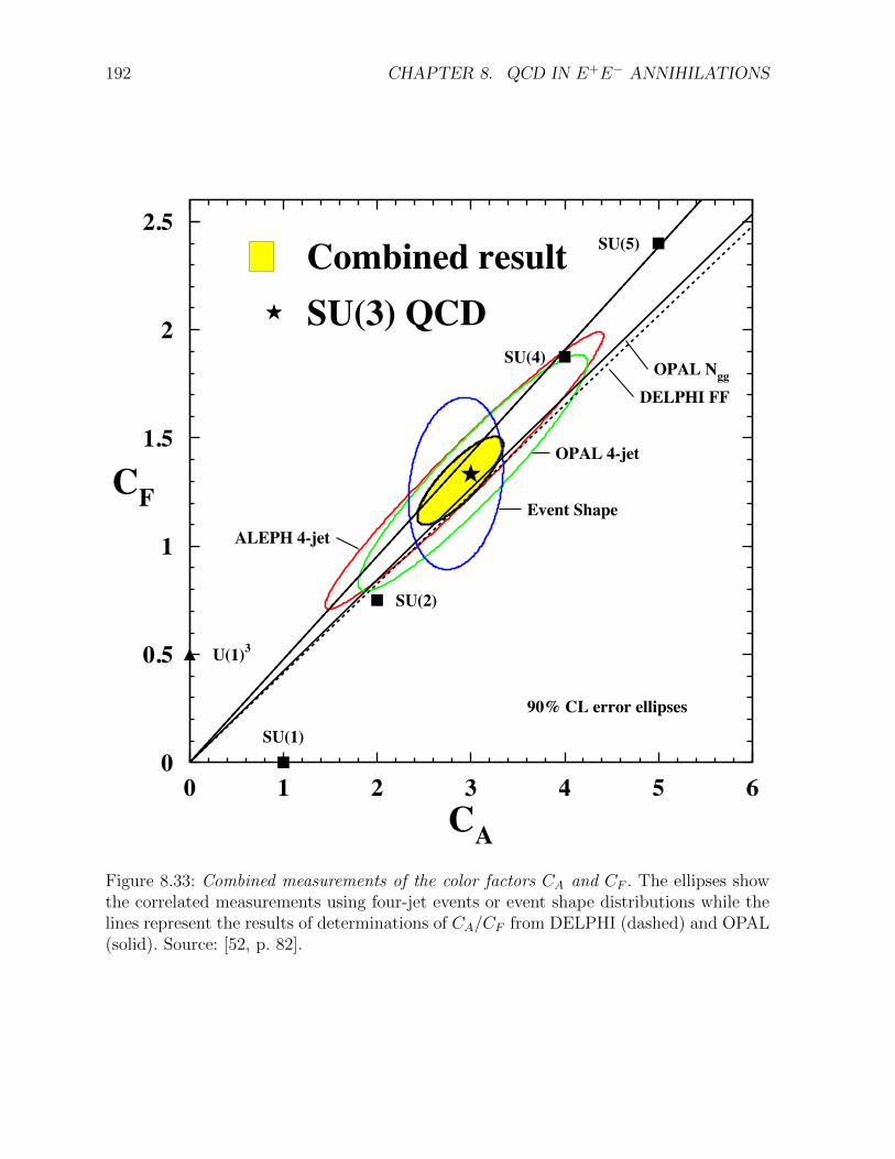
The combined measurements of the QCD color factors are summarized in Fig. 8.33: Four-jet and event shape results have been combined accounting for correlations between themeasurements. In addition, constraints on CA/CF from differences between quark andgluon jets (see p. 177) are included. This yields
CA = 2.89± 0.21
CF = 1.30± 0.09
which is precise to 7% and agrees with the SU(3) values of CA = 3 and CF = 1.33.
8.5 Hadronization
The trouble with hadronization is that perturbative calculations are no longer usefulsince αs ceases to be comparatively small at length scales of about the proton radius.
192 CHAPTER 8. QCD IN E+E− ANNIHILATIONS
CONTENTS
�
���
�
���
�
���
� � � � � � �
�����
�����
�����
�����
��������������������
���������
�����������
����������
�����������
��������
���������
��
��
���������������������
Figure 8.33: Combined measurements of the color factors CA and CF . The ellipses showthe correlated measurements using four-jet events or event shape distributions while thelines represent the results of determinations of CA/CF from DELPHI (dashed) and OPAL(solid). Source: [52, p. 82].

8.5. HADRONIZATION 193
Figure 8.34: Visualization of phenomenological models of hadronization. (LHS) string frag-mentation: JETSET/PYTHIA; (RHS) Cluster fragmentation: HERWIG. Source: [27, p.164]
Perturbative QCD is applicable to the transition from the primary partons to a set offinal state partons. This is pictured as a cascading process that is dominated by thecollinear and soft emissions of gluons and mainly light quark-antiquark pairs. By contrast,phenomenological models are used to describe the non-perturbative transition from thesefinal state partons to hadrons which then may decay according to further models (recallFig. 8.6).
The parameters determining the behavior of the numerical models have to be adjustedusing experimental data. Hadronization can be modeled by string fragmentation (JET-SET/PYTHIA) or cluster fragmentation (HERWIG). For a visualization of this difference,see Fig. 8.34.
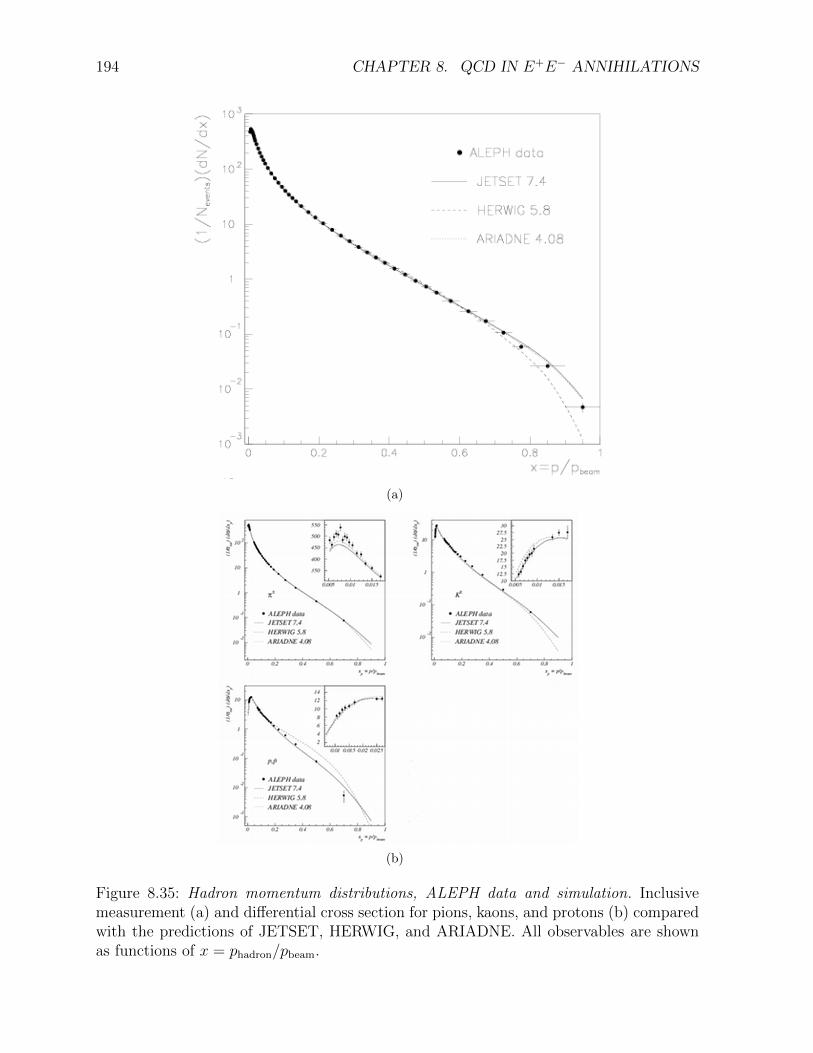
Fig. 8.35 shows comparisons of simulations to ALEPH data for hadron momentum distri-butions of the final state: Fig. 8.35(a) shows simulation and data for an inclusive variableand Fig. 8.35(b) deals with pions, kaons, and protons, respectively.
194 CHAPTER 8. QCD IN E+E− ANNIHILATIONS
(a)
(b)
Figure 8.35: Hadron momentum distributions, ALEPH data and simulation. Inclusivemeasurement (a) and differential cross section for pions, kaons, and protons (b) comparedwith the predictions of JETSET, HERWIG, and ARIADNE. All observables are shownas functions of x = phadron/pbeam.