1

Chapters 2 and 10: Least Squares Regression

Learning goals for this chapter:

Describe the form, direction, and strength of a scatterplot.

Use SPSS output to find the following: least-squares regression line, correlation,

r2, and estimate for σ.

Interpret a scatterplot, residual plot, and Normal probability plot.

Calculate the predicted response and residual for a particular x-value.

Understand that least-squares regression is only appropriate if there is a linear

relationship between x and y.

Determine explanatory and response variables from a story.

Use SPSS to calculate a prediction interval for a future observation.

Perform a hypothesis test for the regression slope and for zero population

correlation/independence, including: stating the null and alternative hypotheses,

obtaining the test statistic and P-value from SPSS, and stating the conclusions in

terms of the story.

Understand that correlation and causation are not the same thing.

Estimate correlation for a scatterplot display of data.

Distinguish between prediction and extrapolation.

Check for differences between outliers and influential outliers by rerunning the

regression.

Know that scatterplots and regression lines are based on sample data, but

hypothesis tests and confidence intervals give you information about the

population parameter.

When you have 2 quantitative variables and you want to look at the relationship

between them, use a scatterplot. If the scatter plot looks linear, then you can do least

squares regression to get an equation of a line that uses x to explain what happens with y.

The general procedure:

1. Make a scatter plot of the data from the x and y variables. Describe the form,

direction, and strength. Look for outliers.

2. Look at the correlation to get a numerical value for the direction and strength.

3. If the data is reasonably linear, get an equation of the line using least squares

regression.

4. Look at the residual plot to see if there are any outliers or the possibility of

lurking variables. (Patterns bad, randomness good.)

2

5. Look at the normal probability plot to determine whether the residuals are

normally distributed. (The dots sticking close to the 45-degree line is good.)

6. Look at hypothesis tests for the correlation, slope, and intercept. Look at

confidence intervals for the slope, intercept, and mean response, and at the

prediction intervals.

7. If you had an outlier, you should re-work the data without the outlier and

comment on the differences in your results.

Association

Positive, negative, or no association

Remember: ASSOCIATON or CORRELATION is NOT the same thing as

CAUSATION. (See chapter 3/2.5 notes.)

Response variable:

Y

Dependent variable

measures an outcome of a study

Explanatory variable:

X

Independent variable

explains or is related to changes in the response variables (p. 105)

Scatterplots:

Show the relationship between 2 quantitative variables measured on the same

individuals

Dots only—don’t connect them with a line or a curve

Form: Linear? Non-linear? No obvious pattern?

Direction: Positive or negative association? No association?

Strength: how closely do the points follow a clear form? Strong or weak or

moderate?

Look for OUTLIERS!

Correlation: measures the direction and strength of the linear relationship between 2

quantitative variables, r. It is the standardized value for each observation with respect to

the mean and standard deviation.

3

1

1

i i

x y

x x y yr

n s swhere we have data on variables x and y for n individuals.

You won’t need to use this formula, but SPSS will.

Using SPSS to get correlation: Use the Pearson Correlation output. Analyze -->

Correlate --> Bivariate (see page 55 in the SPSS manual). The SPSS manual tells you

where to find r using the least squares regression output, but this r is actually the

ABSOLUTE VALUE OF r, so you need to pay attention to the direction yourself. The

Pearson Correlation gives you the actual r with the correct sign.

Properties of correlation:

X and Y both have to be quantitative.

It makes no difference which you call X and which you call Y.

Does not change when you change the units of measurement.

If r is positive, there is a positive association between X and Y

As X increases, Y increases

If r is negative, there is a negative association between X and Y

As X increases, Y decreases

1 1r

The closer r is to –1 or to 1, the stronger the linear relationship

The closer r is to 0, the weaker the linear relationship

Outliers strongly affect r. Use r with caution if outliers are present.

4

Example: We want to examine whether the amount of rainfall per year increases or

decreases corn bushel output. A sample of 10 observations was taken, and the amount of

rainfall (in inches) was measured, as was the subsequent growth of corn.

Amount of Rain Bushels of Corn

3.03 80

3.47 84

4.21 90

4.44 95

4.95 97

5.11 102

5.63 105

6.34 112

6.56 115

6.82 115

The scatterplot:

a) What does the scatterplot tell us? What is the form? Direction? Strength?

What do we expect the correlation to be?

amount of rain (in)

765432

co

rn y

ield

(b

ush

els

)

120

110

100

90

80

70

5

Correlations

amount of rain (in)

corn yield (bushels)

amount of rain (in) Pearson Correlation 1 .995(**)

Sig. (2-tailed) . .000

N 10 10

corn yield (bushels) Pearson Correlation .995(**) 1

Sig. (2-tailed) .000 .

N 10 10

** Correlation is significant at the 0.01 level (2-tailed).

Inference for Correlation:

R = correlation

R2 = % of variation in Y explained by the regression line (the closer to 100%, the

better)

ρ (Greek letter rho) = correlation for the population

When ρ = 0, there is no linear association in the population, so X and Y are

independent (if X and Y are both normally distributed).

Hypothesis test for correlation:

To test the null hypothesis H0: ρ = 0, SPSS will compute the t statistic: 2

2

1

r nt

r,

degrees of freedom = n – 2 for simple linear regression.

b) Are corn yield and rain independent in the population? Perform a test of

significance to determine this.

c) Do corn yield and rain have a positive correlation in the population? Perform

a test of significance to determine this.

This test statistic for the correlation is numerically identical to the t statistic used to test

H0: 1 = 0.

Can we do better than just a scatter plot and the correlation in describing how x and y are

related? What if we want to predict y for other values of x?

6

Least-Squares Regression fits a straight line through the data points that will minimize

the sum of the vertical distances of the data points from the line.

Minimizes 2

1

( )n

i

i

e

Equation of the line is: 0 1ˆ ˆ, with = the predicted liney b b x y y

Slope of the line is: 1

y

x

sb r

s, where the slope measures the amount of change

caused in the predicted response variable when the explanatory variable is

increased by one unit.

Intercept of the line is: 0 1b y b x , where the intercept is the value of the

predicted response variable when the explanatory variable = 0.

Type of line Least Squares Regression

equation of line

slope y-intercept

Ch. 10 Sample

0 1y b b x b1 b0

Ch. 10 Population

(model)

0 1i i iy x 1 0

Using the corn example, find the least squares regression line. Tell SPSS to do

AnalyzeRegression Linear. Put “rain” into the independent box and “corn” into the

dependent box. Click OK.

Coefficientsa

50.835 1.728 29.421 .000 46.851 54.819

9.625 .332 .995 28.984 .000 8.859 10.391

(Constant)

amount of rain (in)

Model

1

B Std. Error

Unstandardized

Coefficients

Beta

Standardized

Coefficients

t Sig. Lower Bound Upper Bound

95% Confidence Interval for B

Dependent Variable: corn yield (bushels)a.

Model Summaryb

.995a .991 .989 1.290

Model

1

R R Square

Adjusted

R Square

Std. Error of

the Estimate

Predictors: (Constant), amount of rain (in)a.

Dependent Variable: corn y ield (bushels)b.

ANOVAb

1397.195 1 1397.195 840.070 .000a

13.305 8 1.663

1410.500 9

Regression

Residual

Total

Model

1

Sum of

Squares df Mean Square F Sig.

Predictors: (Constant), amount of rain (in)a.

Dependent Variable: corn y ield (bushels)b.

7

d) What is the least-squares regression line equation?

The scatterplot with the least squares regression line looks like:

Hypothesis testing for H0: 1 = 0

Test statistic: 1

1b

bt

SE with df = n - 2

SPSS will give you the test statistic (under t), and the 2-sided P-value (under Sig.).

e) Is the slope positive in the population? Perform a test of significance.

f) What % of the variability in corn yield is explained by the least squares

regression line?

g) What is the estimate of the standard error of the model?

amount of rain (in)

765432

corn

yie

ld (

bush

els

)

120

110

100

90

80

70 Rsq = 0.9906

R2 is the percent of

variation in corn yield

explained by the regression

line with rain= 99.06%

8

What do we mean by prediction or extrapolation?

Use your least-squares regression line to find y for other x-values.

Prediction: using the line to find y-values corresponding to x-values that are

within the range of your data x-values.

Extrapolation: using the line to find y-values corresponding to x-values that are

outside the range of your data x-values.

Be careful about extrapolating y-values for x-values that are far away from the x

data you currently have. The line may not be valid for wide ranges of x!

Example: On the rain/corn data above, predict the corn yield for

a) 5 inches of rain

b) 7.2 inches of rain

c) 0 inches of rain

d) 100 inches of rain

e) For which amounts of rainfall above do you think the line does a good job

of predicting actual corn yield? Why?

Cartoon by J.B. Landers on www.causeweb.org (used with permission)

9

Prediction Intervals

Predicting a future observation under conditions similar to those used in the study.

Since there is variability involved in using a model created from sample data, a prediction

interval is better than a single prediction. They’re related to confidence intervals.

Use SPSS.

The 95% prediction interval for future corn yield measurements when rain = 5.11 is

(96.90, 103.14).

Assumptions for Regression:

1. Repeated responses y are independent of each other.

2. For any fixed value of x, the response y varies according to a Normal distribution.

3. The mean response y

has a straight-line relationship with x.

4. The standard deviation of y (σ) is the same for all values of x. The value of σ is

unknown.

How do you check these assumptions?

Scatterplot and R2: Do you have a straight-line relationship between X and

Y? How strong is it? How close to 100% is R2? Hopefully no outliers! (#3)

10

Normal probability plot: Are the residuals approximately normally

distributed? Do the dots fall fairly close to the diagonal line (which is always

there in the same spot)? (#2)

Residual plot: Do you have constant variability? Do the dots on your

residual plot look random and fairly evenly distributed above and below the 0

line? Hopefully no outliers! (#1 and 4)

Residual is the vertical difference between the observed y-value and the

regression line y-value:

ˆi i i i i data lineresidual e y y y a bx y y

Residual plot:

scatterplot of the regression residuals against the explanatory variable (e vs. x)

e-axis has both negative and positive values but centered about e = 0.

the mean of the least-squares residuals is always zero. 0e

Good: total randomness, no pattern, approximately the same number of points

above and below the e = 0 line

Bad: obvious pattern, funnel shape, parabola, more points above 0 than below

(or vice versa)

if you have a pattern, your data does not necessarily fit the model (line) well

0.0 0.2 0.4 0.6 0.8 1.0

Observed Cum Prob

0.0

0.2

0.4

0.6

0.8

1.0

Exp

ecte

d C

um

Pro

b

Dependent Variable: corn yield (bushels)

Normal P-P Plot of Regression Standardized Residual

11

Example: Show a residual plot for the corn/rain data using SPSS.

Outliers:

Outliers are observations that lie outside the overall pattern of the other

observations.

Outliers in the y direction of a scatterplot have large regression residuals (ei)

Outliers in the x direction of a scatterplot are often influential for the regression

line

An observation is influential if removing it would markedly change the result of

the calculation

Outliers can drastically affect regression line, correlation, means, and standard

deviations.

You can draw a second regression line that doesn’t include the outliers—if the

second line moves more than a small amount when the point is deleted or if R2

changes much, the point is influential

Which hypothesis test do you use when?

If you’re not sure whether to use β1 or ρ, here are some guidelines. The test statistics and

P-values are identical for either symbol.

Use If the words are:

β1 Slope, regression coefficient

ρ Correlation, independence

Either β1 or ρ linear relationship

amount of rain (in)

765432

Uns

tand

ardi

zed

Res

idua

l

2.5

2.0

1.5

1.0

.5

0.0

-.5

-1.0

-1.5

-2.0

12

Review of SPSS instructions for Regression: When you set up your regression, you click on:

Analyze-->Regression-->Linear. Put in your y variable for "dependent"

and your x variable for "independent" on the gray screen. Don't hit

"ok" yet though.

Back on the regression gray screen, click on "Plots", and then click on

"normal probability plot." Click "continue" on the Plots gray screen.

Back on the regression gray screen, click on "Save", and then click on

“unstandardized residuals." Click “Individual” under the “Prediction

Interval” section, and adjust the confidence level, if needed. Click

"continue" on the Save gray screen and then "ok" to the big Regression

gray screen.

The prediction interval and the residuals will show up back on the data

input screen. The LICI_1 and UICI_1 give you the prediction interval

lower and upper bounds.

You still won't have a residual plot yet. If you click back to your

data input screen, you now have a new column called "Res_1". To make

the residual plot, you follow the same steps for making a scatterplot:

go to graphs-->scatter-->simple, then put "Res_1" in for y and your x

variable in for x. Click "ok." Once you see your residual plot,

you'll need to double click on it to go to Chart Editor.

On the Chart Editor tool bar, you can see a button that shows a graph

with a horizontal line. Click on that button. Make sure that the y-

axis is set to 0.

14

Example: The scatterplot below shows the calories and sodium content for each of 17

brands of meat hot dogs.

a) Describe the main features of the relationship.

Calories

200180160140120100

Sod

ium

con

tent

600

500

400

300

200

100

b) What is the correlation between calories and sodium?

c) Report the least-squares regression line.

Model Summaryb

.863a .745 .728 48.913

Model

1

R R Square

Adjusted

R Square

Std. Error of

the Estimate

Predictors: (Constant), Caloriesa.

Dependent Variable: Sodium contentb.

Correlations

1 .863**

. .000

17 17

.863** 1

.000 .

17 17

Pearson Correlation

Sig. (2-tailed)

N

Pearson Correlation

Sig. (2-tailed)

N

Calories

Sodium content

Calories

Sodium

content

Correlation is significant at the 0.01 level (2-tailed).**.

15

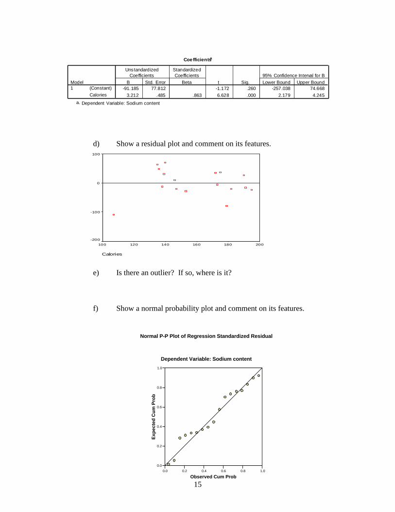
d) Show a residual plot and comment on its features.

e) Is there an outlier? If so, where is it?

f) Show a normal probability plot and comment on its features.

Calories

200180160140120100

Uns

tand

ardi

zed

Res

idua

l

100

0

-100

-200

Coefficientsa

-91.185 77.812 -1.172 .260 -257.038 74.668

3.212 .485 .863 6.628 .000 2.179 4.245

(Constant)

Calories

Model

1

B Std. Error

Unstandardized

Coefficients

Beta

Standardized

Coefficients

t Sig. Lower Bound Upper Bound

95% Confidence Interval for B

Dependent Variable: Sodium contenta.

0.0 0.2 0.4 0.6 0.8 1.0

Observed Cum Prob

0.0

0.2

0.4

0.6

0.8

1.0

Ex

pe

cte

d C

um

Pro

b

Dependent Variable: Sodium content

Normal P-P Plot of Regression Standardized Residual

16

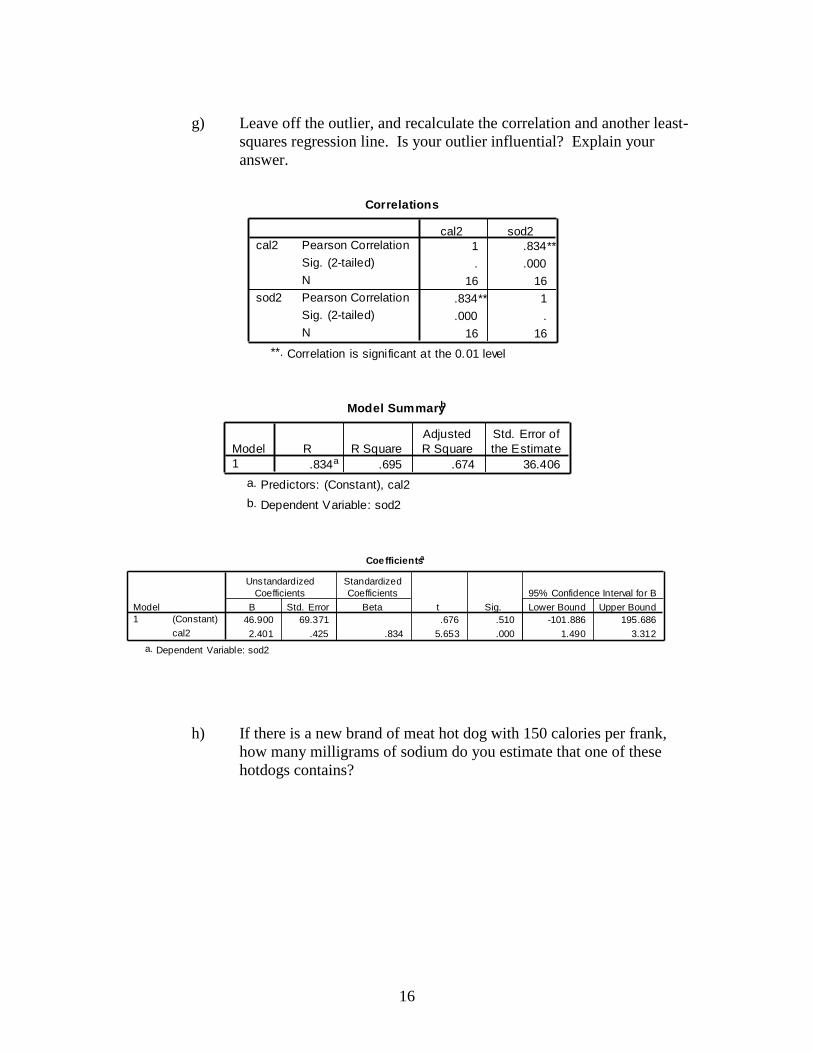
g) Leave off the outlier, and recalculate the correlation and another least-

squares regression line. Is your outlier influential? Explain your

answer.

h) If there is a new brand of meat hot dog with 150 calories per frank,

how many milligrams of sodium do you estimate that one of these

hotdogs contains?

Correlations

1 .834**

. .000

16 16

.834** 1

.000 .

16 16

Pearson Correlation

Sig. (2-tailed)

N

Pearson Correlation

Sig. (2-tailed)

N

cal2

sod2

cal2 sod2

Correlation is significant at the 0.01 level

(2-tailed).

**.

Model Summaryb

.834a .695 .674 36.406

Model

1

R R Square

Adjusted

R Square

Std. Error of

the Estimate

Predictors: (Constant), cal2a.

Dependent Variable: sod2b.

Coefficientsa

46.900 69.371 .676 .510 -101.886 195.686

2.401 .425 .834 5.653 .000 1.490 3.312

(Constant)

cal2

Model

1

B Std. Error

Unstandardized

Coefficients

Beta

Standardized

Coefficients

t Sig. Lower Bound Upper Bound

95% Confidence Interval for B

Dependent Variable: sod2a.