characterisation of laser-accelerated proton beams
TRANSCRIPT

Max-Planck-Institut fur Quantenoptik
Characterisation of Laser-AcceleratedProton Beams
Malte Christoph Kaluza
Vollstandiger Abdruck der von der Fakultat fur Physik der Technischen Universitat Munchenzur Erlangung des akademischen Grades eines
Doktors der Naturwissenschaften
genehmigten Dissertation.
Vorsitzender: Univ.-Prof. Dr. Manfred KleberPrufer der Dissertation: 1. apl. Prof. Dr. Jurgen Meyer-ter-Vehn
2. Univ.-Prof. Dr. Dr. h.c. Alfred Laubereau
Die Dissertation wurde am 14.06.2004 bei der Technischen Universitat Munchen ein-gereicht und durch die Fakultat fur Physik am 23.07.2004 angenommen.


Contents
1 Introduction 1
2 Laser-Plasma Interaction at Relativistic Laser Intensit ies 52.1 Interaction of Laser Light with Plasma Electrons . . . . . .. . . . . . . 6
2.1.1 Treatment of a Single Electron in the Laser Field . . . . .. . . . 62.1.2 Collective Effects of Plasma Electrons . . . . . . . . . . . .. . . 11
2.2 Electron Acceleration Mechanisms in a Plasma . . . . . . . . .. . . . . 152.2.1 Electron Acceleration at the Critical Surface . . . . . .. . . . . . 152.2.2 Electron Acceleration in Underdense Plasma . . . . . . . .. . . 16
2.3 Electron-Beam Transport Through Overdense Plasma . . . .. . . . . . . 182.4 Proton-Acceleration Mechanisms . . . . . . . . . . . . . . . . . . .. . . 19
2.4.1 Proton Acceleration at the Target Front Side . . . . . . . .. . . . 192.4.2 TNSA-Mechanism for Proton Acceleration from the Target Rear
Side . . . . . . . . . . . . . . . . . . . . . . . . . . . . . . . . . 22
3 Experimental Setup 293.1 The Multi-Terawatt Titanium:Sapphire Laser System ATLAS . . . . . . . 293.2 Laser-Pulse Improvements by means of Adaptive Optics . .. . . . . . . 34
3.2.1 Smoothing of the Near-Field Beam Profile . . . . . . . . . . . .343.2.2 Correction of the Laser-Pulse Wave Front . . . . . . . . . . .. . 353.2.3 Measurement of the Intensity Distribution in the Focal Plane . . . 37
3.3 Control and Characterisation of the ASE Pedestal . . . . . .. . . . . . . 393.3.1 Pockels Cells used as Optical Shutters . . . . . . . . . . . . .. . 403.3.2 System of Pockels Cells in ATLAS . . . . . . . . . . . . . . . . 403.3.3 Measurement of Level and Duration of the ASE Prepulse .. . . . 42
4 Proton and Ion Diagnostics 454.1 Ion Detection with CR 39 Nuclear Track Detectors . . . . . . .. . . . . 454.2 Time-Of-Flight Detector . . . . . . . . . . . . . . . . . . . . . . . . . .47
4.2.1 Setup of the Detector . . . . . . . . . . . . . . . . . . . . . . . . 474.2.2 Measurement of Ion Spectra . . . . . . . . . . . . . . . . . . . . 48
4.3 Thomson Parabola . . . . . . . . . . . . . . . . . . . . . . . . . . . . . 504.4 Spatial Profile of the Proton Beam . . . . . . . . . . . . . . . . . . . .. 55
5 Proton Acceleration in the Experiment 575.1 Experimental setup . . . . . . . . . . . . . . . . . . . . . . . . . . . . . 575.2 Proton Spectra for Different Target Thicknesses . . . . . .. . . . . . . . 595.3 Proton Spectra for different ASE Prepulse Durations . . .. . . . . . . . 62
I

5.3.1 Measurements with a constant laser intensity . . . . . . .. . . . 625.3.2 Influence of the laser intensity . . . . . . . . . . . . . . . . . . .635.3.3 Correlated Changes in the Spatial Profiles of the Proton Beam . . 64
5.4 Angularly Resolved Measurement of the Proton Spectra . .. . . . . . . . 675.4.1 Changes in the Experimental Setup . . . . . . . . . . . . . . . . 675.4.2 Measurement of Proton-Energy Spectra and Beam Profiles . . . . 685.4.3 Determination of the Energy-Resolved Divergence of the Protons 705.4.4 Measurement with Different Prepulse Durations . . . . .. . . . . 71
5.5 Summary of the Experimental Observations . . . . . . . . . . . .. . . . 74
6 Simulations with MULTI -FS 756.1 Motivation for Hydro Simulations . . . . . . . . . . . . . . . . . . .. . 756.2 The 1-D Hydrodynamic Code MULTI-FS . . . . . . . . . . . . . . . . . 766.3 Details of the Simulations . . . . . . . . . . . . . . . . . . . . . . . . .. 776.4 Simulation Results from MULTI-FS . . . . . . . . . . . . . . . . . . .. 786.5 Summary of the MULTI-FS Simulations . . . . . . . . . . . . . . . . .. 82
7 1-D Simulations for Rear-Side Proton Acceleration 837.1 Description of the Simulation Code . . . . . . . . . . . . . . . . . .. . 83
7.1.1 Set of Equations Solved by the Code . . . . . . . . . . . . . . . . 847.1.2 Initial Conditions . . . . . . . . . . . . . . . . . . . . . . . . . . 847.1.3 Calculation of the Electrostatic Potential . . . . . . . .. . . . . . 857.1.4 Acceleration of the Proton Distribution . . . . . . . . . . .. . . 867.1.5 Derivation of the Proton-Energy Spectrum . . . . . . . . . .. . . 87
7.2 General Results from the Simulation Code . . . . . . . . . . . . .. . . . 887.2.1 Comparison with the Analytical Model . . . . . . . . . . . . . .897.2.2 Acceleration of the Proton Distribution . . . . . . . . . . .. . . 917.2.3 Influence of an Initial Rear-Side Density Gradient . . .. . . . . . 92
7.3 Conclusion . . . . . . . . . . . . . . . . . . . . . . . . . . . . . . . . . 93
8 Discussion of the Experimental Results 958.1 Free-Streaming Electron Propagation in the Target . . . .. . . . . . . . . 95
8.1.1 Approximations for the Assumption of a Free-Streaming ElectronBeam . . . . . . . . . . . . . . . . . . . . . . . . . . . . . . . . 95
8.1.2 Comparison of Simulation Results with Experimental Data . . . . 978.2 Relevance of Electron-Transport Effects for Proton Acceleration . . . . . 100
8.2.1 The Fast-Electron Transport Code . . . . . . . . . . . . . . . . .1018.2.2 Simulation Results from the Fast-Electron TransportCode . . . . 1038.2.3 Application of Simulation Results for Proton Acceleration . . . . 1058.2.4 Comparison between Experimental Results and Front-Side Pro-
ton Acceleration . . . . . . . . . . . . . . . . . . . . . . . . . . 1078.2.5 Conclusions from the Target-Thickness Scan . . . . . . . .. . . 109
8.3 Results Obtained from the Angular Scan . . . . . . . . . . . . . . .. . . 1118.3.1 Description of the Proton Acceleration with 3-D PIC codes . . . . 1118.3.2 Conclusions . . . . . . . . . . . . . . . . . . . . . . . . . . . . . 113

9 Summary and Perspectives 1159.1 Possible Future Experiments on Proton Acceleration . . .. . . . . . . . 1169.2 Suggestions Numerical Simulations of Laser-Plasma Interactions . . . . . 117
A Setup of a Synchronised Probe Beam 119A.1 Experimental Setup . . . . . . . . . . . . . . . . . . . . . . . . . . . . . 119A.2 Generation of two fs-Probe Beams Separated by Several ps. . . . . . . . 121A.3 Interferometry Using a Wollaston-Prism . . . . . . . . . . . . .. . . . . 122A.4 Preplasma Generation Using a Synchronised Nd:Glass Laser . . . . . . . 123A.5 Channel Formation in the Preformed Plasma . . . . . . . . . . . .. . . . 125
A.5.1 Plasma Channels in Self-Emission . . . . . . . . . . . . . . . . .126A.5.2 Interferometrical Pictures of Plasma Channels . . . . .. . . . . . 127
Bibliography 129
P Publication List 139
Danksagung 147

Chapter 1
Introduction
The development of ultrahigh-power laser systems using thetechnique of chirped-pulse-amplification (CPA) [1] has sparked an enormous scientific activity in the field of laser-plasma interaction. Beyond intensities of a few times 1018W/cm2, the motion of electronsin the electromagnetic field of the laser becomes relativistic, as the electron velocity ap-proaches the speed of light within only one oscillation period, and a large variety of newphenomena opens up. Worldwide, laser facilities delivering pulses with peak powers inexcess of 1 petawatt (1PW=1015W) have either been comissioned during the last fewyears [2–4] or are presently under construction. Such lasersystems have pushed the limitof achievable intensities beyond 1021W/cm2 [5].
When laser pulses with these intensities interact with any kind of target material, therising edge of the pulse is already sufficiently intense to transform matter into the plasmastate. The main part of the pulse then interacts with a highlyionised and heated plasma.Due to collective effects of the freed electrons, such a plasma can support electric fieldsin excess of 1012V/m. These fields are higher by several orders of magnitude comparedto conventional particle accelerators that usually operate at 108 V/m. Due to the higherfields the acceleration length for particles in the energy range of several 100’s of MeV isof the order of 1mm at most [6]. Therefore, high-power lasersare a promising alternativeto conventional RF-accelerators.
During the last decade, a dramatic increase in particle energies accelerated in laser-plasma experiments could be witnessed. Primarily, the laser light efficiently couples itsenergy into the formation of collimated electron beams withpeak kinetic energies in therange from several 100keV to more than 200MeV [6–10]. In secondary processes, itis possible to generateγ−rays in the MeV-range [9, 11], to accelerate protons [12–17],and also heavy ions [18] to MeV-energies, and to generate neutrons from fusion reactions[9, 19, 20]. Although most of the proof-of-principle experiments were carried out withlarge-scale Nd:Glass-laser systems generating pulses at arepetition rate of∼ 1 shot/hourat the 100TW to 1PW level, small-scale laser systems in the 1. . .20terawatt (TW) regimeoperating at a much higher repetition rate allow experiments for the investigation of thephysics underlying the associated acceleration processesin much greater detail. Using the2-TW laser facility ATLAS at Max-Planck Institut fur Quantenoptik operating at 10Hz, itwas possible for the first time to generate positrons with a table-top laser [21].
Although the generation of fast ions in the energy range of a few 10’s or 100’s of keVhas already been observed in the late 1970’s [22–25], the generation of MeV-proton beams
1
2 Chapter 1 Introduction
during the interaction of high-intensity CPA-laser pulseswith thin foils has attracted agreat deal of attention due to the unique properties of such beams. Independent of thetarget material, a strong and well-collimated proton signal is observed in the experiments.These protons originate from water vapor and hydrocarbon contaminations on the targetsurfaces, as it has been observed in experiments carried outin the framework of the LosAlamos Helios program [26].
Using the NOVA-PW laser at Lawrence Livermore National Laboratory [27], atotalnumber of 2×10¹³ protons has been accelerated to kinetic energies above 10MeV [15].The initial proton-pulse length is determined by the laser pulse duration (τL = 500fs in thisexperiment), and it is emitted from a spot of∼ 100-µm diameter from the rear surface ofthe target. This yields an initial proton current as high as 6.4×10⁶ A and a proton-powerdensity in excess of 1018W/cm2, what is higher by several orders of magnitude comparedto conventional accelerators. Furthermore, the rear-sideaccelerated proton beam exhibitsan extraordinary low emittance and an almost ideal laminar flow as a consequence of theacceleration process [28–30]. Such beams are therefore well suited for the imaging ofµm-scale structures on the rear surface of the target. By appropriately shaping the target rearsurface, the focusing of a proton beam has recently been demonstrated [31]. During theinteraction of this beam with a secondary target, isochoricheating of the secondary-targetmaterial to temperatures of 20eV has been observed1. As protons having MeV-energiescan penetrate dense matter, they can be used to probe highly overdense plasmas that arenon transparent for optical light [32]. Due to their electric charge the protons are alsodeflected by magnetic and electric fields in the plasma and carry information about thefield distributions in the highly overdense regions [33,34]. Furthermore, laser-acceleratedprotons are envisaged as a possible ignition beam [35] in thefast-ignitor scenario forinertial confinement fusion [36].
For all the applications mentioned above, the generation ofproton beams with control-lable parameters such as energy spectrum, brightness, and spatial profile is crucial. Hence,for the reliable generation of proton beams, the physics underlying the acceleration pro-cess has to be understood as accurately as possible. After the first proof-of-principleexperiments [12–16], systematical studies were carried out to examine the influence oftarget material and thickness [37–39]. To establish the influence of the main laser pa-rameters such as intensity, pulse energy, and duration overa wide range, results fromdifferent laser systems have to be compared, as each system covers a small parameterrange only. Besides these parameters, strength and duration of the laser prepulse due toamplified spontaneous emission (ASE) play an important role, too [37]. Until now, a de-tailed investigation has not been carried out but is expected to play a significant role in theacceleration process [40,41].
Besides the influence of the experimental parameters mentioned above, the origin ofthe fastest protons is still debated. There are at least two acceleration scenarios ableto explain the occurance of MeV-protons during the interaction of high-intensity laserswith thin foils. (i) These protons may come from thefront surface of the target, i.e. theside irradiated by the laser [12–14] or (ii) from therear surface [15, 18, 42]. Recent
1In laser-plasma physics, it is convenient to express temperatures not in Kelvin, but in eV. The equivalenttemperature to the quasi-temperature of 1eV is 11.600K.

Chapter 1 Introduction 3
results indicate that both mechanisms act simultaneously [43,44], in accordance with thepredictions of multi-dimensional particle-in-cell (PIC)codes [17,45].
Special attention has also been paid to the spatial profile ofthe proton beam emittedfrom the target. Using the solid-state nuclear track detector CR 39, “ring”-like structureshave been observed in different experiments [13, 14, 46]. These structures were the basisfor conflicting interpretations about the origin of the proton beam.
Aiming at a global picture for the physics underlying the proton acceleration process,the influence of as many experimental parameters as possiblehas to be understood. Alsothe role and suitability of the diagnostics used in different experiments has to be inves-tigated to be able to compare the results and interpretations. Therefore, this work is fo-cused on the characterisation of proton beams accelerated in high-intensity laser-solidinteractions and the influence of the different experimental parameters on the accelerationprocess.
During the course of this thesis, the following new and important aspects were discov-ered and described:
1. For the first time, a controlled variation of the laser-prepulse pedestal due to am-plified spantaneous emission was achieved by implementing an ultra-fast Pockelscell into the laser chain. The prepulse was characterised interms of intensity andduration.
2. Due to this unique possibility, the influence of the laser prepulse duration on thelaser-driven acceleration of protons could be studied in great detail. It was found tohave a huge effect on the emitted energy spectra of the protons [47].
3. By a controlled variation both of the prepulse duration and the thickness of thetarget foil used in the experiment, a clear distinction between the two differentacceleration regimes mentioned above was possible. Furthermore, the controlledgeneration of a proton population stemming from the rear side of the target waspossible for the first time.
4. By comparing the experimental results with numerical simulations, a quantitativeexplanation of the associated effects was possible. It was found that the prepulse-induced changes in the target properties not only influence the rear-side proton ac-celeration by the formation of an initial ion-density gradient as claimed in [37],but also the density distribution in the target itself strongly influences the electronpropagation, which in turn affects the rear-side proton acceleration [48].
The results described in this thesis both have a high relevance for a comparison of existingexperimental results as well as for future experiments aiming at an optimisation of theacceleration process. The thesis is structured as follows:
• Chapter 2 gives an overview over the physics of laser-plasmainteractions at rela-tivistic laser intensities. After a description of the interaction of a single electronwith the laser field, the occurance of collective effects of electrons in the plasma

4 Chapter 1 Introduction
are discussed. They give rise to charge separation in the plasma and generate quasi-static electric fields. These fields are responsible for the acceleration of protons andlight ions to MeV-energies. The two acceleration scenariosfrom the two differenttarget surfaces are described.
• Chapter 3 describes the ATLAS-laser system that was used for the experiments.The control of the laser prepulse by means of an ultra-fast Pockels cell and thesignificant enhancement of the laser focusability by adaptive optics are described indetail, as their comissioning and characterisation were major parts of this work [49]and were crucial for the feasibility of experiments on proton acceleration.
• Chapter 4 deals with the diagnostics used to characterise the proton beam acceler-ated during the laser-plasma interaction in terms of energyspectrum, spatial diver-gence, and angular distribution.
• Chapter 5 presents the experimental results investigatingthe dependence of theproton-beam properties on different experimental parameters as target thickness,prepulse duration, laser-pulse energy and emission angle.The profound effect ofthese parameters on the acceleration process could be demonstrated [47].
• To qualitatively describe the effect of the prepulse, hydrodynamic simulations usingthe code MULTI -FS [50] were carried out. The results from these simulations arediscussed in chapter 6.
• Chapter 7 presents a 1-dimensional computer code that was newly developed withinthe course of this work. It describes the rear-side proton acceleration driven by ahot-electron population accelerated by the laser on the target front side. The codeis used to include prepulse-induced changes as target expansion and formation of aplasma-density gradient at the target rear side in the description of the accelerationprocess and to obtain a more detailed insight into the underlying physics.
• Chapter 8 draws conclusions from the comparison of the experimental results withthe predictions from numerical simulations and theory. A distinction between twoproton populations accelerated on either of the two target surfaces is possible. Itmanifests the strong influence of target thickness and prepulse duration on these twomechanisms. A numerical code is used to describe the influence of the fast-electrontransport on the rear-side acceleration of protons. Furthermore, the angularly re-solved measurements are found to match the predictions madeby three-dimensionalparticle-in-cell (PIC) simulations [45], giving an insight into the distributions of theelectron density and the acceleration fields at the target rear surface.
• Finally, chapter 9 summarises this work and gives a perspective for the future, sug-gesting further experiments and numerical investigationsconcerning the accelera-tion of protons and light ions in relativistic laser-plasmainteraction.
• Appendix A describes the setup of a novel, synchronised 2-colour probe beam thatwas set up during the course of this thesis and that was used for interferometricside-view images taken during the laser-target interaction.
• In appendix P, the publications about the most important parts of this work areattached.

Chapter 2
Laser-Plasma Interaction at RelativisticLaser Intensities
During the interaction of ultra-short laser pulses having peak intensities in excess of1018W/cm2 with solid targets, the main part of the laser pulse with the highest inten-sities interacts with a highly ionised and strongly preheated plasma on the target frontside. This preplasma has been formed by the unavoidable low-intensity prepulse pedestalof the laser due to amplified spontaneous emission (ASE) and by the leading edge of themain pulse itself. In this preplasma, the electrons are accelerated to velocities close tothe speed of light by the laser fields and therefore their motion is dominated by relativis-tic effects. At these “relativistic” intensities, a large fraction of the laser-pulse energy isconverted into kinetic energy of relativistic electrons. They are expelled from the focalregion of the laser pulse due to its ponderomotive force and leave behind a space chargeof positive ions close to thefront surfaceof the target. Furthermore, the electrons havingkinetic energies in the MeV-range are capable of propagating through the target. A strongspace-charge field is generated at therear surfacedue to electrons that have escaped thetarget. The electric fields arising from these regions of charge separations on both targetsurfaces vary on a time scale that is much longer than the laser period that dominatesthe electron motion. These quasi-static fields are capable of accelerating ions to kineticenergies in the MeV-range. To understand and interpret these two different mechanismsunderlying the ion acceleration at the front and rear side ofthe target, the interaction ofthe laser pulse with the plasma electrons has to be describedfirst.
This chapter starts with the interaction of a laser-light wave of relativistic intensity witha single electron. Subsequently, effects are discussed that arise from the collective be-haviour of a large number of electrons, when the laser pulse interacts with the preplasmaincluding the different collective electron-acceleration processes. Finally, the two differ-ent ion-acceleration mechanisms are introduced.
5

6 Chapter 2 Laser-Plasma Interaction at Relativistic Laser Intensities
2.1 Interaction of Laser Light with Plasma Electrons
2.1.1 Treatment of a Single Electron in the Laser Field
First, the interaction of a single electron with a plane laser-light wave is investigated.The light wave is assumed to propagate in~ex-direction and to be linearly polarised in~ey-direction.
Description of the Laser Field
The light wave of the laser is described by its vector potential, ~A(x, t), that is parallel tothe~ey-direction and varies only in space,x, and time,t: 1
~A = ~ey ·A0sin(kLx−ωLt), (2.1)
whereωL/2π is the laser-light frequency,kL = 2πηr/λL the wave number,λL = 2πc/ωL
the laser-wave length in vacuum,ηr the refractive index, andc the speed of light. In theabsence of any electrostatic potential,Φel, the electric and magnetic fields,~EL and~BL, areobtained from
~EL = −∂~A∂t
= ~E0cos(kLx−ωLt), with ~E0 = ~ey ·ωLA0 and (2.2)
~BL = ~∇×~A = ~B0cos(kLx−ωLt), with ~B0 = ~ez ·kLA0 = ~ezηrE0
c. (2.3)
In vacuum, whereηr = 1, the laser intensity,IL, which is the magnitude of the Poyntingvector,~S, averaged over a laser period,TL = 2π/ωL , what is denoted by〈. . .〉, can bewritten as
IL = 〈|~S|〉 =1µ0
〈| ~EL × ~BL|〉 =ε0c2
E20 , (2.4)
whereµ0 is the permeability andε0 the permittivity of the vacuum.
Interaction of a Single Particle with the Laser Field
The interaction of an electron with charge−eand rest massme with external electric andmagnetic fields,~E and~B, is described by itsequation of motion
d~pdt
=ddt
(γme~v) = −e(
~E +~v×~B)
, (2.5)
where~v and~p are velocity and momentum of the electron, respectively.γ = 1/√
1−β2 =1/√
1−v2/c2 =√
1+(p/mec)2 is the relativistic Lorentz factor,β = v/c. Multiplying
1Note that all field quantities of the light wave depend on space, x, and time,t, what will be omitted forclarity.

2.1 Interaction of Laser Light with Plasma Electrons 7
eq. (2.5) with~p and using~p· (~v×~B) = 0 and~p·d~p = 12dp2, one obtains theevolution of
the kinetic energy, Ekin = mec2(γ−1), of the electron to
dEkin
dt= mec
2 dγdt
= −e~E ·~v. (2.6)
In the classical regime, i.e. for velocitiesv c, whereγ ≈ 1, the electron motionis dominated by the electric field, as the magnetic term is smaller by a factor ofv/cand in the first order can be neglected. Integrating the equation of motion (2.5) forthis case with initial conditionsx0 = 0,y0 = 0, andv0 = 0 leads to the velocity~v =~ey ·eE0/ωLme ·sin(kLx−ωLt) and the displacementy = eE0/ω2
Lm· [cos(kLx−ωLt)−1]of the electron. In the classical case, the electron oscillates driven by the external electricfield with amplitudesy0 = eE0/ω2
Lme andv0 = eE0/ωLme parallel to the electric fieldonly2.
The amplitude of the velocity,v0, approachesc, when the so-callednormalised vectorpotential
a0 =eE0
ωLmec=
eA0
mec(2.7)
approaches unity. In this case, a purely classical description is no longer valid. Usinga0,the amplitudes of the electric and magnetic fields can be rewritten as
E0 =a0
λL·3.21×1012V
m·µm and (2.8)
B0 =a0
λL·1.07×104T ·µm. (2.9)
The laser-light intensity,IL, is given by
IL =a2
0
λ2L
·1.37×1018W/cm2 ·µm2. (2.10)
The normalised vector potential,a0, delimits the interaction of laser light with matterinto three regimes. Fora0 1, the electron motion is classical and the regime is callednon-relativistic. Fora0 ≈ 1, the electron approaches the speed of light already duringa laser-half cycle and the interaction has to be treated fully relativistic, for a0 1, theregime is called ultra-relativistic. For a wave length ofλL = 790nm, the normalisedvector potentiala0 equals 1 for an intensity of 2.2×10¹⁸W/cm2. In the experimentsdescribed in this thesis, the maximum intensity on target was IL = 1.5×10¹⁹W/cm2 witha wave length ofλL = 790nm. This results in a normalised vector potential ofa0 = 2.6.
In the relativistic regime, the solution of the equation of motion (2.5) leads to differentresults compared to the classical case [51–53]. Using the vector potential from eq. (2.1)
2As the amplitude of the velocity scales with the inverse particle mass, it is obvious that during the interac-tion with a plasma the laser mainly couples to the electrons in the first place, as their mass is much lowerthan the mass of even the lightest ions. Except for extremelyhigh intensities (see below), the ions in aplasma are not directly affected by the laser fields but the forces of the laser light are mediated by theplasma electrons.

8 Chapter 2 Laser-Plasma Interaction at Relativistic Laser Intensities
and the expressions (2.2) and (2.3) for the electric and magnetic field one finds
dpy
dt= e
dAdt
=⇒ py−eA= C1, (2.11)
where∂~A/∂t = d~A/dt−(~v·~∇)~A,~v×(~∇×~A) =~∇(~v·~A)−(~v·~∇)~A, and∂~A/∂y= ∂~A/∂z= 0were used. The constantC1 is thefirst invariant of the electron motion. It is related tothe electron’s initial momentum in~ey−direction.
Together with eq. (2.6) and considering that~E0‖~ey and~B0‖~ez, one obtains from eq. (2.5)
dpx
dt= −evyB0 = mec
dγdt
=⇒ γ− px
mec= C2. (2.12)
C2 is thesecond invariantof the electron motion. Usingγ2 = 1+(p/mec)2, one finds thefollowing relation between longitudinal and transversal momentum,px andpy:
px
mec=
1−C22 +(py/mec)2
2C2. (2.13)
Considering an electron that is at rest att = 0 and atx = 0, i.e.~p = 0, when the electricfield is maximal, one findsC1 = 0 andC2 = 1. This leads to
py = eAy and (2.14)
Ekin = cpx =p2
y
2me, (2.15)
and one obtains the following form of the relativistic Lorentz factor for a single electronin a laser wave:γ = 1+ a2/2. To derive thex− andy−coordinates of the electron,Φ =kLx−ωLt and dΦ/dt = vxkL −ωL = ωL(βx−1) = −ωL/γ are used, what leads to
~p = γmed~rdt
= γmed~rdΦ
· dΦdt
= −meωLd~rdΦ
. (2.16)
Using eqs. (2.14) and (2.15), the integration of thex− andy−component of eq. (2.16)leads to the spatial components of the electron trajectory:
x =c
ωL
a20
4
(
Φ− 12
cos(2Φ)
)
and (2.17)
y =c
ωLa0
(
1−cosΦ)
. (2.18)
While they−component is identical to the classical case, the electron is strongly pushedforward in laser direction fora0 ≥ 1. This forward motion in the laboratory frame consistsof a drift in laser direction with the velocity
~vD =
⟨
xt
⟩
=a2
0
4+a20
c·~ex (2.19)

2.1 Interaction of Laser Light with Plasma Electrons 9
arising from the first part in eq. (2.17). This drift velocityapproachesc for a0 → ∞. Thesecond part describes a rapid oscillation of the electron in~ex−direction with twice thefrequency as in~ey−direction. This gives rise to a “figure-8” motion of the electron in aframe of reference co-moving with~vD.
For the case of an infinitely long laser pulse with an infinite lateral extension, the elec-tron motion in the laboratry frame is sketched in Fig. 2.1 (a). For the case of a laser pulse
Figure 2.1: Relativistic electron motion in the laser field. In (a), the laser is a plane wave ofinfinite length. In (b), the laser has a finite duration and is either a plane wave (red line) or it isfocused to a Gaussian spot of finite diameter (green line).
of finite duration as shown in Fig. 2.1 (b), where eqs. (2.14) and (2.15) are still valid,the electron is pushed forward by the laser as in (a). But whenthe pulse is over, theelectron comes to a stop again (red line). In this case, the electron is only displaced inlaser direction but gains no net energy. However, the electron can be ejected from a laserfocus of finite diameter, if this diameter is comparable to orsmaller than the amplitude ofthe electron’s quiver motion. It leaves the focus under an angle, θ, to the laser axis witha finite velocity (green line) by so-calledponderomotive scattering(see below) [54–57].This can be understood qualitatively, as the electron starting on the laser axis, where thefields are maximal, is displaced sideways during the first laser-half cycle into regions ofreduced intensity. Thus the restoring force acting on the electron is smaller, when thefields change sign. Hence, it does not return to its initial position in the next laser-halfperiod, and finally leaves the focus with a finite velocity.
The Ponderomotive Force
If one is not interested in the detailed trajectory but only the final energy and the scatteringangle of the electron, an elegant description of the acceleration is obtained by introducingthe ponderomotive force,~Fpond, of the laser acting on the electron [58,59]. To derive thisnon-linear force, one again starts from the equation of motion (2.5), first assumingγ ≈ 1for the classical case:
md~vdt
= −e(~E +~v×~B). (2.20)

10 Chapter 2 Laser-Plasma Interaction at Relativistic Laser Intensities
In the first order, only contributions that depend linearly on the electric field,~E(x, t) =~Es(~r) ·cos(ωLt), are used, where~Es(~r) contains the spatial dependence. For the velocity,~v1, and the displacement,δ~r1, of the electron from its initial position,~r0, one finds
~v1(~r0) = − emeωL
~Es(~r0) ·sin(ωLt) =d~rdt
and (2.21)
δ~r1(~r0) =e
meω2L
~Es(~r0) ·cos(ωLt). (2.22)
To proceed to the second order, the electric field,~E(~r), is expanded around the electron’sinitial position,~r0, to
~E(~r) = ~E(~r0)+ (δ~r1 ·~∇) ~E∣
∣
∣
~r=~r0
+ . . . (2.23)
Using now only terms that quadratically depend on the electric field and deriving themagnetic field,~B1, from Maxwell’s equation~∇×~E = −∂~B/∂t, what leads to~B1(~r0) =
−ω−1L
~∇× ~E∣
∣
∣
~r=~r0
·sin(ωLt), the second-order equation of motion reads
med~v2
dt= −e
[
(
δ~r1(~r0) ·~∇)
~E(~r0)+~v1(~r0)× ~B1(~r0)
]
= − e2
meω2L
[
(
~Es(~r0) ·~∇)
~Es(~r0) ·cos2(ωLt)+
+~Es(~r0)×(
~∇× ~Es(~r0))
·sin2(ωLt)
]
. (2.24)
Temporally averaging over the fast oscillations of the laser field (〈sin2(ωLt)〉= 〈cos2(ωLt)〉=12) and using~Es× (~∇× ~Es) = 1
2~∇(E2
s )− (~Es ·~∇)~Es, this finally leads to
~Fpond= me
⟨
d~v2
dt
⟩
= − e2
4meω2L
~∇(E2s ). (2.25)
A fully relativistic description gives an additional factor of 1/〈γ〉 [60], whereγ is alsoaveraged over the fast oscillations of the laser field
~Fpond= − e2
4〈γ〉meω2L
~∇(E2s ). (2.26)
According to this equation, an electron is expelled from high-intensity regions of the laserfocus along the gradient of the laser-intensity distribution, which is proportional toE2
s .Finally, the scattering angle,θ, is determined by the ratio of transversal and longitudinalmomentum of the electron [55] that are determined by eq. (2.14) and eq. (2.15):
θ = arctan
(
py
px
)
= arctan
(√
2γ−1
)
. (2.27)
This relation has been verified experimentally by Mooreet al. [54], where the scatteringof single electrons from the laser focus was observed.
2.1 Interaction of Laser Light with Plasma Electrons 11
Note that all the relations derived up to this point describethe interaction of a singleelectron in the electromagnetic fields of a laser pulse. Any electrostatic potentials arisingfrom laser-induced charge separations during the interaction of the laser with a plasmahave been neglected so far. It will be shown in the next section, how the situation changes,when such effects are taken into account.
Up to now, only electrons were concerned, while the ions wereassumed to form animmobile, positively charged background. Due to their muchhigher rest mass, the laserintensities presently available are by far not high enough to trigger a relativistic ion quivermotion in the laser field. The relativistic threshold for protons with massmp ≈ 1836me
is ata0 = 1836 and therefore at an intensity ofILλ2L = 18362 ·1.37×1018W/cm2·µm2 =
4.62×1024W/cm2·µm2, which is far beyond the present laser technology. However,col-lectiveeffects of a large number of plasma electrons interacting with an intense laser pulsegive rise to strong electric fields that vary on the time scaleof the pulse duration and notof the laser period. On these much longer time scales, also the ions in the plasma canbe accelerated to MeV-energies. These collective effects of the plasma electrons will bediscussed in the next section.
2.1.2 Collective Effects of Plasma Electrons
This section concentrates on collective effects of the plasma electrons that occur duringthe interaction with laser pulses of relativistic intensities (a0 ≥ 1). While collective elec-tron acceleration mechanisms in a plasma are discussed in section 2.2, this section isdedicated to the relativistic equation of motion in a plasma, Debye-shielding, the plasmafrequency, and relativistic effects concerning the propagation of laser pulses in a plasma.
Relativistic Equation of Motion in a Plasma
To derive the relativistic equation of motion in a plasma, the electrons are treated as afluid at zero temperature with density and velocity distributions,ne(~r , t) andve(~r , t), thatdepend on space and time. Due to their significantly higher rest mass, the plasma ions areassumed to form an immobile, positively charged background.
As in the case for a single electron, the behaviour of this electron fluid is describedby the equation of motion as eq. (2.5), the electric and magnetic fields can now also bemodified by charge distributions and currents in the plasma
~B = ~∇×~A, (2.28)
~E = −~∇Φel−∂~A∂t
, (2.29)
what leads to an equation of motion of the form
(
∂∂t
+~v·~∇)
~p = −e
[
− ∂~A∂t
−~∇Φel +~v× (~∇×~A)
]
. (2.30)

12 Chapter 2 Laser-Plasma Interaction at Relativistic Laser Intensities
Using the relationsγ =√
1+(p/mec)2,~∇γ = (2γ)−1 ·~∇(p/mec)2, and~v× (~∇ × ~p) =
mec2~∇γ− (~v·~∇)~p, one obtains therelativistic equation of motion of the plasma[61] to
∂∂t
(
~p−e~A)
−~v×~∇×(
~p−e~A)
= ~∇(
eΦel− γmec2)
. (2.31)
This equation has a trivial solution~p = e~A and thereforee~∇Φel = mec2~∇γ, in which theponderomotive force,mec2~∇γ, is balanced by the electrostatic force,e~∇Φel, arising fromthe laser-induced charge separation in the plasma. This implies γ =
√1+a2, what dif-
fers from the expression for a single electron derived in section 2.1.1, and leads to theponderomotive potential in a plasma,
Φpond= mec2(γ−1) = mec
2(√
1+a2−1)
. (2.32)
The ponderomotive potential depends on the local laser intensity that scales witha2. Inthe focus of the laser pulse, where the intensity is maximal anda= a0, the ponderomotivepotential can be expressed in units of the laser intensity,IL , and the laser wave length,λL ,according to eq. (2.10):
Φpond= 511keV×(√
1+ILλ2
L
1.37×10¹⁸W/cm2·µm2−1
)
. (2.33)
Debye Shielding
One of the key characteristics of a plasma is its tendency to shield externally appliedelectric fields. The differently charged particles arrangein a way that an electric field ofopposite orientation is generated that tends to cancel the external field on a macroscopicscale, where the plasma appears to be quasi-neutral. On a microscopic scale, the positiveions are surrounded by plasma electrons that shield the electric potential of the ions. Fora single ion with charge,Ze, this shielding modifies the pure Coulomb potential by anexponential drop [59]
Φion(r) =1
4πε0
Zer·exp
(
− rλD
)
(2.34)
with the characteristic shielding length,λD, that depends on the temperature,Te, and thedensity,ne, of the surrounding plasma electrons:
λD =
√
ε0kBTe
nee2 . (2.35)
λD is called theDebye lengthof the plasma andkB denotes the Boltzmann constant. In anundisturbed plasma, charge neutrality is provided on scales larger than the plasma Debyelength.

2.1 Interaction of Laser Light with Plasma Electrons 13
Light Propagation in a Plasma
If the plasma electrons are displaced from the positive ion background by an externalperturbation, a restoring force builds up due to the electric fields arising from the chargeseparation. When the perturbation is over, the electrons start to oscillate around the posi-tion of charge equilibrium with a characteristic frequency, ωpe, that only depends on thedensity,ne, of the plasma electrons [58]:
ωpe =
√
nee2
ε0me. (2.36)
ωpe is called theelectron plasma frequency.The plasma electrons can also follow peri-odic external perturbations, that are varying with frequenciesω < ωpe. A light wave withω < ωpe cannot propagate in a plasma, as the electrons shield the oscillating light field. Ifthe electric field of the external perturbation is that strong that the electron quiver velocityapproachesc within the oscillation, the effective electron mass,γme increases, what inturn changes the electron plasma frequency. Due to the variation of the effective electronmass during an oscillation cycle, the electron motion becomes unharmonious. Then theelectron plasma frequency is given by
ωpe =
√
nee2
ε0〈γ〉me, (2.37)
where〈γ〉 is averaged both over the fast oscillation of the laser field and locally overa large number of electrons. However, when the external frequency exceedsωpe, theelectrons are too inert to follow the varying field, and the external wave can propagate inthe plasma. If on the other hand an electromagnetic wave withfrequencyωL propagatesthrough a plasma density gradient, it is stopped at that electron density,ncr, where thelight frequency,ωL , matches the local plasma frequency,ωpe. This density is called thecritical plasma density
ncr =ε0〈γ〉meω2
L
e2 =1.11×1021cm−3
λ2L
· 〈γ〉 ·µm2. (2.38)
For a laser-wave length ofλL = 790nm and low intensities, i.e.〈γ〉 ≈ 1, the critical densityis ncr = 1.79×1021cm−3. Plasmas with electron densities above this limit are calledovercritical, below this density they are referred to asundercritical.
The propagation of an electromagnetic wave with frequencyωL in an underdenseplasma is described by theplasma dispersion relation
ω2L = k2
Lc2 + ω2pe. (2.39)
Using the refractive index,ηr, of the plasma, that is defined by
ηr =
√
1−(
ωpe
ωL
)2
=
√
1−(
ne
ncr
)
, (2.40)

14 Chapter 2 Laser-Plasma Interaction at Relativistic Laser Intensities
the group and phase velocity of the electromagnetic wave,vgr andvph, in the plasma read
vgr =∂ωL
∂k= ηr ·c and vph =
ωL
k=
1ηr
·c. (2.41)
As the refractive indexηr in a plasma withne < ncr is always smaller than 1, the groupvelocity is smaller and the phase velocity larger thanc.
The intensity dependence of the refractive indexηr via the Lorentz factor, that isaveraged both over the fast laser oscillations and a large number of plasma electrons,〈γ〉 = (1+ a2)1/2, has several consequences for the propagation of laser pulses of rela-tivistic intensities in plasmas.
• The plasma frequency decreases for increasing laser intensity. Therefore, a plasmalayer with an electron densityne, that is overcritical and therefore non transparentfor a sub-relativistic light wave witha0 1, can become transparent for a laserpulse witha0 ≤ 1, when the condition
ε0ω2Lme
e2 < ne <ε0ω2
Lme
e2 ·√
1+a20 (2.42)
is fulfilled. This phenomenon is calledself-induced transparency[62].
• If a laser pulse with amoderate intensity, that is on the one hand low enough to betreated classically but on the other hand sufficiently high to significantly enhancethe ionisation degree of the plasma by optical field ionisation, the electron densityin the center of the focus is increased due to the ionisation,while the density re-mains unchanged outside the focus. This leads to a lower refractive index in thecenter of the beam, what in turn increases the phase velocity, vph = c/ηr, of thelaser wave in the center compared to the wings of the focus. Therefore, the plasmaacts as a negative lens, defocusing the laser beam. This effect is calledionisationdefocusing.When arelativistic laser pulse is focused into a plasma, the averaged electron mass,γme, increases the more during the oscillation in the laser field, the higher the localintensity is. This leads to a reduction of the refractive index on the laser axis com-pared to the wings of the focus. If this effect dominates the ionisation defocusing,the plasma acts as a positive lens further increasing the intensity compared to thefocusing in vacuum. This effect is calledrelativistic self-focusing. Furthermore,the electrons are ponderomotively scattered out of the center of the focus where theintensity is higher, decreasing the local electron density. This effect, that furtherenhances the laser-beam focusing, is referred to asponderomotive self-focusing.The power threshold above which relativistic self-focusing dominates over the ion-isation defocusing is given by [63]
PRSF= 2mec2
e4πε0mec3
e·(
ncr
ne
)
= 17.4GW·(
ncr
ne
)
, (2.43)
wheremec2/e= 511kV is the voltage corresponding to the electron rest energy and4πε0mec3/e= 17kA is the Alfven current [64], which is the maximum current thatcan be transported through vacuum (see below).
2.2 Electron Acceleration Mechanisms in a Plasma 15
2.2 Electron Acceleration Mechanisms in a Plasma
When a high-intensity laser pulse interacts not only with a single electron, as it was dis-cussed in section 2.1.1, but with a plasma, the situation becomes much more complex as alarge variety of nonlinear effects associated with the collective behaviour of the electronsopens up. It turns out that a fraction of the plasma electronscan very effectively – in totalnumber as well as in kinetic energy – be accelerated by high-intensity laser pulses. Afraction of several tens of percent of the laser pulse energycan be converted into electronsin the MeV-range forming adirectedelectron beam – in contrast to the pure heating of aplasma resulting in an almostisotropicvelocity distribution. As all these different collec-tive effects potentially influence each other, a description of the whole picture as completeas possible can only be achieved by using numerical simulations.
Depending on the experimental conditions, different acceleration mechanisms can be-come dominant. In general, they can be divided into two groups. First, electrons areaccelerated at or close to the surface of the overcritical plasma layer, where the laser pulseis stopped and partly reflected. These effects play a role in experiments with solid tar-gets, where such a layer exists. Second, electrons are accelerated in underdense-plasmaregions, as they occur in gas targets or in long-scale lengthpreplasmas in front of a solidtarget. These effects become dominant, when the laser pulsecan propagate through un-derdense plasma regions over a distance that is much longer compared to its minimaldiameter in the focus.
2.2.1 Electron Acceleration at the Critical Surface
In experiments with solid targets, the intrinsic laser prepulse due to amplified spontaneousemission is intense enough to generate a preplasma at the target front side, in which theelectron density rises from 0 in vacuum to the solid density (∼ 1023cm−3) over a scalelength that depends on the prepulse characteristics. When the main pulse is incident onthe overdense plasma surface (∼ 1021cm−3) that is parallel to the initial target surface, itis partially reflected. As the beam cannot propagate beyond this overcritical surface, thefield gradient is maximal here and it is directed normal to theovercritical surface. Theponderomotive force directed along the steepes field gradient drives electrons perpendic-ular to the surface of the overcritical-plasma layer into the target. While this surface isinitially parallel to the target surface, it is deformed during the interaction with the laseras the laser pulse pushes electrons and hence also the critical surface sideways and in for-ward direction. This effect is referred to as laser hole boring. In the context of relativisticlaser-plasma interaction, it has been identified in 2-D PIC simulations [65]. Due to thiseffect, the direction of electron acceleration is no longeronly perpendicular to the targetsurface, but occurs in a direction between target normal andlaser direction [66]. Themean energy or the effective temperature,kBTe, of the electron population accelerated inthat way can be estimated by the ponderomotive potential of the laser to
kBTe = mec2(
√
1+a20−1
)
16 Chapter 2 Laser-Plasma Interaction at Relativistic Laser Intensities
= 0.511MeV·(√
1+ILλ2
L
1.37×10¹⁸W/cm2µm2−1
)
. (2.44)
This relation has first been deduced from PIC simulations carried out by S. Wilkset al.[67] and verified experimentally by G. Malkaet al. [8]. Typically, a fraction ofη ≈ 25%of the laser energy,EL, is converted into electrons having such a Boltzmann temperature[9]. Laser pulses from ATLAS, delivering an energy ofEL = 850mJ on the target withλL = 790nm at an averaged intensity ofIL = 1.5×10¹⁹W/cm2, generate an electronpopulation with a quasi-temperature ofkBTe ≈ 920keV. The total number,Ne, of thispopulation can be estimated to be the total energy of the population divided by their meanenergy:
Ne ≈ηEL
kBTe= 1.44×10¹². (2.45)
Brunel Heating
In this scenario, ap-polarised3 laser pulse is focused under oblique incidence onto asolid target with a steep density gradient, i.e. a short scale length,Lp, of the order of thelaser-wave length [68]. As in vacuum, the transverse electric field of the laser accelerateselectrons sideways. While in vacuum the electrons would oscillate symmetrically aroundthe laser axis, in regions close to the critical surface of the solid the electrons only expe-rience the electric field of the laser in areas of undercritical density. They are acceleratedtowards the vacuum in the first laser-half cycle, turn round and are accelerated into thesolid, where they feel no restoring forces any more as the laser fields cannot penetrateinto overdense regions. Via this mechanism the electrons can gain energy and enter thesolid along the direction of the gradient, but the acceleration is only effective for steepgradients (otherwise the necessary differences in the forces acting on the electron duringthe two laser-half cycles are too small).
2.2.2 Electron Acceleration in Underdense Plasma
Laser Wake-Field Acceleration
When a short laser pulse is focused into an underdense plasma, the ponderomotive forceacting at the leading edge of the pulse expells electrons from the focal region. This chargeseparation excites a plasma wave that follows the laser pulse in its wake and copropagateswith the group velocity,vgr = c·ηr < c, of the laser pulse in the plasma. The longitudinalelectric field in the plasma wave can trap electrons that can gain a large amount of kineticenergy, when they travel with the wave. This acceleration mechanism, that is called laserwakefield acceleration (LWFA), was proposed by T. Tajimaet al. [69]. It is most efficient,
3For p-polarisation, the electric field vector of the laser pulse incident on the target under oblique incidencelies in the plane defined by thek-vector of the wave and the target normal. Fors-polarisation, the electricfield vector is perpendicular to this plane. Here, the laser electric field vector has no component parallelto the target normal, as it is the case forp-polarisation.

2.2 Electron Acceleration Mechanisms in a Plasma 17
when the laser-pulse duration is half as long as a period of the plasma oscillation, i.e. ifτL = π/ωpe. The problem is to trap electrons efficiently; large trapping occurs when theplasma wave breaks, i.e. when groups of wave electrons move faster than the wave’s phasevelocity.
Direct Laser Acceleration
During the interaction of a relativistic laser pulse with a plasma of undercritical densityself-focusing of the laser pulse can occur, when the power threshold, eq. (2.43), is passed.This reduces the focal diameter of the laser and increases the intensity compared to thefocusing in vacuum. A plasma channel is formed along the laser axis, that extends overa distance of many Rayleigh lengths of the vacuum-laser focus. In this channel, the pon-deromotive forces of the laser radially expell electrons and additionally drive a strongelectron current along the channel. This leads to the formation of strong radial electricfields due to the lack of plasma electrons in the channel and strong azimuthal magneticfields due to the high current. An electron running under small initial pitch angles to theaxis of the channel is bent back by the strong electric and magnetic fields and starts to os-cillate in these fields. If this electron oscillation is in resonance with the Doppler-shiftedlaser-light oscillation, and if the phases between electron and laser field match, the elec-tron can gain a large amount of energy directly from the laserfields. This mechanism iscalled direct laser acceleration (DLA) and has been described by Z. M. Sheng, A. Pukhov,and J. Meyer-ter-Vehn [70,71]. In an experiment carried outby C. Gahn at the MPQ usingthe ATLAS laser system, it has been demonstrated clearly [10]. It is capable of acceler-ating electrons to very high energies, but it requires a longregion of underdense plasmaas present in a gas jet or in a long-scale length preplasma that a plasma channel can buildup. For the “ideal” conditions of a gas jet, where a self-focused channel of 400-µm lengthwas observed, a conversion efficiency of 5% was measured in [10].
To estimate the efficiency of this mechanism in experiments with solid targets, thepossible length over which a plasma channel can form, has to be determined. This is thelength of the region, where the electron density is above thedensity for self focussing,given by eq. (2.43) and below the critical density,ncr, where the laser pulse is reflected.Depending on the preplasma conditions, this region can be asshort as several tens ofmicrometers only for very short laser prepulses or as long asseveral 100’s ofµm for verylong and intense prepulses. In the experiments of this thesis, this length was of the orderof 10µm to 50µm. Hence, it can be estimated that the efficiency of electron accelerationvia DLA will be less than 5% in the experiments reported here.For the case of a long-scale length preplasma formed by a second, synchronised ns-laser pulse as in [72], theefficiency of this acceleration mechanism might increase again. In appendix A, someresults from an experiment are described, where electrons were accelerated in a plasmachannel via direct laser acceleration. In this experiment,a long-scale length preplasmawas generated by a ns-Nd:Glass laser pulse, the channel extended over more than 400µm.
18 Chapter 2 Laser-Plasma Interaction at Relativistic Laser Intensities
Concluding Remarks
Although these are only some examples for different possible scenarios to accelerate elec-trons on the target front side, multi-dimensional PIC-simulations show that the electroninjection into the target mainly occurs in a direction between target normal direction andlaser propagation direction [66]. Here, the deformation ofthe critical surface due to hole-boring is important, too. The direction of the electron injection into the target also dependson the preplasma conditions [73]. For scale lengths above 10. . .15µm, the direction ofthe electron beam is mainly directed in laser forward direction, for scale lengths below3. . .5µm, the electron injection into the target is mainly parallelto the target normal direc-tion. Recent experiments carried out at MPQ showed a clear distinction between the twoacceleration directions, one in laser direction the other one in target normal direction [74].
By these effects, a large number of high-energetic electrons is generated capable ofpropagating through the target. During their passage through the overdense part of thetarget, collective effects of the beam electrons play a role, too. They will be discussed inthe next section.
2.3 Electron-Beam Transport Through Overdense Plasma
In the last section, mechanisms to accelerate∼1012 electrons (cf. eq. 2.45) with a temper-ature of∼1MeV were described. As the acceleration process occurs within the laser pulseduration only, the corresponding hot-electron current entering the target is of the order of106 A. This value exceeds by far the Alfven limit for electron currents,IA = βγ ·17kA[64]. No electron current above this limit can freely propagate in vacuum, as for such acurrent the beam electrons are forced on bent trajectories by the self-induced magneticfield that no net current above this limit can be transported in the initial beam direction.However, in a plasma the transport of currents above the Alfven limit is possible, whenthe hot-electron current is compensated locally by a suitable return current. This returncurrent is driven by electric fields induced by magnetic fieldbuild-up due to the fast-electron current itself and by the charge separation in the target. While the hot-electronbeam is generated at the critical density,ncr, and the beam density is of the same order(∼1021cm−3), the electron density of the return current,nret, is of the order of the soliddensity (∼1023cm−3). Consequently, the return current consists of a slow driftof thebackground electrons. For conductors, the return current can be carried by the free elec-trons. In insulators however, free electrons first have to begenerated by field or collisionalionisation [75]. These ionisation processes strongly reduce the energy of the hot-electronbeam.
The configuration of two counter-streaming electron currents is highly unstable withrespect to the Weibel instability [76], as small local perturbations in the current densitiesthat violate the exact balancing of the two currents give rise to azimuthal magnetic fieldsgenerated by the arising net current that tend to pinch this net current and to expell thereturn current out of this beam filament. This can lead to the formation of beam filaments,each carrying up to one Alfven current, that is cylindrically surrounded by a return current

2.4 Proton-Acceleration Mechanisms 19
almost cancelling the magnetic field outside the filament. When two of these filamentscoalesce afterwards due to residual attraction, a part of the energy carried by the hot-electron current is converted into transversal heating of the surrounding plasma, until thecurrent carried by the merged filament is reduced to one Alfv´en current again. If thiseffect, that was described by M. Honda [77], sets in, it leadsto a significant dissipation ofenergy, the electron beam undergoes so-called anomalous stopping.
While the distance between the filaments described above is on a sub-µm scale, the elec-tron beam as a whole having an initial diameter of several micrometers can undergo beampinching, too. This can be understood qualitatively as follows. The background plasmais ohmically heated by the return current [41, 75] leading toa non uniform temperaturedistribution of the background plasma producing a spatial variation of the resistivity of theplasma that strongly depends on the temperature [78]. This gives rise to a spatial variationof the electric field driving the return current that generates an azimuthal magnetic fieldthat can pinch the electron beam as a whole [79]. This scenario is investigated in detail inchapter 8.2 using a fast-electron-transport code developed by J. J. Honrubia [80] .
2.4 Proton-Acceleration Mechanisms
As described at the end of section 2.1.1, thedirect interaction of protons and all the moreheavier ions with laser light of presently achievable intensities is by far not strong enoughto accelerate these ions to MeV-energies. However, the plasma electrons can mediate theforces of the laser fields to the ions by the generation of strong and quasi-static electricfields arising from local charge separations. These fields can be of the same magnitude asthe fast-oscillating laser fields, but they vary on a time scale comparable to the laser-pulseduration giving the ions a significantly longer time to be accelerated.
In this section, the two main proton-acceleration scenarios will be described, that canboth provide sufficiently strong electric fields over a sufficiently long time. According tothese two scenarios, protons can either be accelerated in the laser focus at thetarget frontside, where the ponderomotively expelled electrons leave behind a positive space chargeof ions, or at thetarget rear side, where the electrons, that have been accelerated by thelaser on the front side and have propagated through the target, form a thin Debye-sheath,that also provides strong and long-lasting electric fields.
2.4.1 Proton Acceleration at the Target Front Side
The first possible mechanism accelerates protons at the front side of the target in the vicin-ity of the laser focus due to electrostatic fields arising from the ponderomotive expulsionof plasma electrons from regions of high laser intensities.The front-side proton acceler-ation has recently been studied by Y. Sentokuet al. using a 1-D PIC code [81]. In thesesimulations, the laser pulse is focused into a preplasma having aµm-scale length, that hasbeen formed by the intrinsic prepulse of the laser. This preplasma is assumed to be quasi-neutral before the arrival of the main pulse, i.e. electron and ion densities balance each

20 Chapter 2 Laser-Plasma Interaction at Relativistic Laser Intensities
other:ne0(x) ≈ ni0(x), as it is sketched in Fig. 2.2 (a). When the main pulse of relativistic
Figure 2.2: Electron and ion densities,ne0 andni0, at the target front side immediately before (a)and during (b) the interaction of a relativistic laser pulsewith the preformed plasma. Due to theponderomotive force, electrons are piled up at the laser-pulse front, until the electrostatic potentialof the charge separation,Φel, balances the ponderomotive potential of the laser,Φpond.
intensity with a normalised vector potentiala0 > 1 arrives at the relativistic critical sur-face, electrons are ponderomotively expelled out of the focal region, until the electrostaticpotential,Φel, arising from the charge separation balances the ponderomotive potential,Φpond, of the laser, that was given in eq. (2.32), what leads to
Φel ≈ Φpond= mec2(γ−1) = mec
2(√
1+a2−1)
. (2.46)
This situation is shown in Fig. 2.2 (b). When a single proton experiences this potential,it can gain a maximum kinetic energy equal to the potential difference. This holds true,as long as the acceleration field lasts long enough for the proton to be accelerated to thisenergy. The life-time of the field can be estimated to be the laser pulse duration,τL . Thenecessary proton-acceleration time,τacc, that has to be compared to the field duration,τL ,will now be derived – following the paper by Sentoku.
The 1-D equation of motion for a proton in the front-side acceleration field,Ex, reads
mpdvp
dt=
dEp
dx= eEx, (2.47)
wheremp andvp are proton mass and velocity, respectively, andEp = 12mpv2
p is its kineticenergy. To integrate this equation, it is assumed that the electrostatic field,Ex, is constantwith an averaged value ofEx0/2 over an acceleration lengthxmax, that will be determinedbelow. Then the kinetic energy as a function of distance,x, is given by
Ep(x) = eEx0
2x. (2.48)
As the maximum proton energy reached at the end of the acceleration length,xmax, equalsthe ponderomotive potential, i.e.Ep(xmax) = Φpond= kBTe, and as the maximum value ofthe electric field isEx0 ≈ kBTe/eλD, (see next section), the acceleration length isxmax =2λD. Note that this differs from the assumptions made by Sentoku [81], wherexmax ≈

2.4 Proton-Acceleration Mechanisms 21
λD/2 andEx0 ≈ 2mec2〈γ〉/eλD were assumed. With these values, the protons do not gainthe maximum energy equal to the ponderomotive potential. Therefore, the different valuesas described above are used here to fulfill this requirement and to obtain a coherent pictureof the front-side acceleration.
To obtain the acceleration time,τacc, the relation
mp
2
(
dxdt
)2
= eEx0
2x → dt =
dx√
(eEx0/mp)x(2.49)
is used and integrated fromx = 0 to xmax = 2λD, whereEx0 was assumed to be constant:
τacc=
2λD∫
0
dx√
(eEx0/mp)x=
√
8mpλD
eEx0≈
√
8mpλ2D
kBTe. (2.50)
The Debye length at the critical density, that is given in eq.(2.38), can be written as
λ2D =
ε0kBTe
ncre2 =kBTe
ω2Lme〈γ〉
=kBTe
4π2mec2 ·λ2
L
〈γ〉 . (2.51)
This finally leads to the following expression for the proton-acceleration time
τacc=
√
8mp
me〈γ〉· TL
2π≈ 20× TL
√
〈γ〉, (2.52)
whereTL denotes the laser period. For the ATLAS conditions (TL=2.63fs and〈γ〉 ≈ 2.8),one findsτacc≈ 32fs, what is significantly shorter than the laser-pulse duration of τL =150fs. It can therefore be concluded that during the interaction of the laser pulse withthe preplasma on the target-front side, a proton can be accelerated to the maximal energydetermined by the ponderomotive potential of the laser. Note that eqs. (2.51) and (2.52)differ from [81], whereλD ∼ λL was assumed. The acceleration time predicted by Sentokufor the ATLAS conditions would be 70fs. Nevertheless, both estimates forτacc are wellbelow the laser-pulse duration in the experiments described in this thesis.
Further investigations of the front-side acceleration process carried out by Sentoku in[81] with 1-D PIC simulations revealed an additional collective effect of the protons, thatincreases the maximum proton energies. Immediatetly afterthe interaction with the laserpulse, a proton front with a very sharp density peak is formed. As the local electrontemperature is too high (and thus the local Debye length too long) to shield the strongelectrostatic repulsion forces within this front, it explodes afterwards further acceleratingthe fastest protons. In the simulations an increase of the maximum proton velocity by afactor of 1.5 is observed. This further increases the maximum proton energy by a factorof (1.5)2.
Taking all these considerations into account, an analytical estimate for the maximumenergy of the front-side accelerated protons for laser pulses withτL ≥ τacc can be given.It is
Ep,front = (1.5)2 ·kBTe
= 1.15MeV·(√
1+ILλ2
L
1.37×10¹⁸W/cm2 ·µm2−1
)
, (2.53)
22 Chapter 2 Laser-Plasma Interaction at Relativistic Laser Intensities
and forIL = 1.5×10¹⁹W/cm2 andλL = 790nm as in the experiments described in chap-ter 5, the maximum energy for protons accelerated at the front side of the target is
Ep,front = 2.1MeV. (2.54)
All the assumptions and conclusions discussed above are based on 1-D geometry. How-ever, as the laser focus in a real experiment has a finite diameter and as the charge-separation sheath in which the acceleration occurs will no longer be plane but convex-shaped, the protons will consequently be accelerated in a large opening angle around thetarget normal direction, which is the initial direction of the electron density gradient asdiscussed above.
2.4.2 TNSA-Mechanism for Proton Acceleration from the Targ et Rear Side
The second possible mechanism also providing strong and slowly-varying electric fieldsfor an effective proton and ion acceleration acts at the target rear surface. In this section,the physical picture of the mechanism will be described and an analytical description forthe evolution of the electrical field driving the acceleration is presented.
The Physical Picture
MeV-electrons that have been generated in the laser focus propagate through the targetas discussed above. After the fastest electrons have left the target at the rear side, astrong electrostatic potential is built up due to the chargeseparation in the vicinity ofthe rear-side target-vacuum boundary. As soon as the subsequently arriving electronspass this boundary, they are held back and forced to return into the target. Due to thismechanism an electron sheath is formed at the rear surface ofthe target. An estimationfor the initial electric-field strength shows that the fieldsare by far strong enough to ioniseatoms at the target rear surface (see below). These ions can subsequently be acceleratedby the same fields. Due to unavoidable contaminations of water or pump-oil vapor onthe target surfaces, the favorably accelerated ion speciesare protons, as they have thehighest charge-to-mass ratio. They leave the target together with comoving electronsforming a quasi-neutral plasma cloud. As the plasma densityin this cloud quickly dropsafter the detachment from the target and as the temperature remains high in this cloud,recombination effects are negligible for propagation lengths in the range of several meters[82]. The situation for the rear-side acceleration mechanism is sketched in Fig. 2.3.
The electric-field lines are parallel to the normal vector ofthe target rear surface andalso the ion acceleration is aligned along this direction. Therefore, the mechanism iscalledTarget-Normal-SheathAcceleration (TNSA). It has first been described by Snavelyand Wilks [15,17] in short-pulse experiments using the Nova-Petawatt laser at LawrenceLivermore National Laboratory, where the emission of protons normal to both rear sur-faces of a wedge-shaped target was observed. Since then it has been widely accepted as apossible mechanism to accelerate protons to kinetic energies well above 1MeV.

2.4 Proton-Acceleration Mechanisms 23
targetfront sideblow-offplasma
rear sideelectron sheath
quasi-neutralplasma cloud
laser pulse
lD,front lD,rear
electrons
ions
Figure 2.3: Sketch of the TNSA-mechanism. The laser pulse coming from the left is focused intoa preplasma on the target front side having a long Debye length, λD,front, which has been formedby the laser prepulse. Electrons are accelerated in the laser focus. They propagate through thetarget setting up an electrical field due to charge separation, when they leave the target at the rearsurface, forming a thin electron sheath with a very short Debye length,λD,rear. This electrical fieldionizes atoms at the rear surface and accelerates them in target normal direction. The ions leavethe target in a quasi-neutral cloud together with comoving electrons.
The pyhsical model underlying the TNSA-mechanism has already been described inthe early 1970’s for the acceleration of ions using ns-laserpulses [83–85]. The significantdifferences to present-day experiments are the much shorter laser-pulse durations, themuch higher electron temperatures, and the associated different temporal evolution fo theelectric fields driving the acceleration process. For long-pulse experiments, the plasma atthe target rear surface slowly expands. Due to the expansionof the positive ion distribution(see below), the electric fields at the ion front are reduced during the expansion. Therefore,the acceleration becomes almost ineffective already during the laser pulse duration. Forshort-pulse experiments however, the life-time of the acceleration field is dominated bythe laser pulse duration and not by the ion expansion itself.The acceleration process isterminated, when the laser pulse is over.
The TNSA-mechanism works as well at the target front surface, as the MeV-electronsthat were initially accelerated in laser direction, are reflected at both target surfaces dueto the space charge fields. They can travel through the targetto and fro several times,while they loose their energy and quickly spread out sideways, heating up the bulk of thetarget. Protons accelerated at the target-front side by TNSA leave the target along thefront-side normal direction into the front-side half space4. This effect has been observedby G. D. Tsakiriset al. [24] and recently by E. Clarket al. [13]. Due to the much longer
4Note that the front-side acceleration described in the lastsection accelerates the protonsinto the target,while the TNSA-mechanism described here accelerates ions into the front half space, i.e.away fromthetarget.
24 Chapter 2 Laser-Plasma Interaction at Relativistic Laser Intensities
scale length in the front-side blow-off plasma, that has been generated by the laser pre-pulse, the electric fields are much lower here. Although thepotential differenceis equalfor both target surfaces, the electric fields, that are proportional to thepotential gradient,are inversly proportional to the Debye length in the plasma sheaths at each target surface.As the potential difference and the electric fields are only kept up as long as the elec-tron temperature remains high, ions accelerated at the target-front side gain much lowerenergies by the TNSA-mechanism.
The initial TNSA-model by S. Wilks [17] provides an analytical estimate only for theelectric field at the beginning of the acceleration process,which was also derived in ear-lier papers that described the plasma expansion into a vacuum driven by a hot electronpopulation. The evolution during the expansion of the proton distribution could only bestudied with multi-dimensional computer codes, that quickly reached the limits of eventhe most powerful computer systems. P. Mora recentyl provided an analytical descriptionof the evolution of the peak electric field in the expanding plasma cloud during the wholeacceleration process for planar geometry [86]. These formulas can exactly be reproducedby numerical but time-consuming simulations, as it will be shown in chapter 7. If one isinterested in the peak energy of the protons only, these formulas can be used to accuratelypredict the peak proton energies achieved during the acceleration process from the targetrear side.
Estimation for the Initial Electric Field
To derive an expression for the initial electric field,E0, at the target rear side, the simplestcase of a pre-ionised hydrogen plasma with a step-like hydrogen-density distribution atthe rear surface,x = 0, is investigated. When an electron population with a Boltzmann-like temperature,Te, and an initial electron density,ne0, exits the target at the rear side, anelectrostatic potential,Φel(x), is generated that is in thermal equilibrium with the electron-density distribution:
ne(x) = ne0·exp
(
eΦel(x)kBTe
)
. (2.55)
Furthermore, the Poisson equation provides another potential-dependence of the chargedensities, and one obtains
∂2
∂x2 Φel(x) = −ρ(x)ε0
=ene0
ε0·
exp
(
eΦel(x)kBTe
)
−1 for x≤ 0, (I)
exp
(
eΦel(x)kBTe
)
for x≥ 0, (II)
(2.56)
whereρ(x) is the total charge distribution andnp = ne0 for x≤ 0 is assumed, which impliescharge neutrality forx→−∞. Case (II) can be integrated analytically to
eΦel(x)kBTe
= −2ln
(
1+x√
2eEλD
)
−1 forx≥ 0. (2.57)

2.4 Proton-Acceleration Mechanisms 25
Here,eE = 2.71828. . . denotes the basis of the natural logarithm. From this expression forthe potential, the electric field,Efr, that has its peak value at the target-vacuum interface,x = 0, at the timet = 0, can be derived by
Efr = − ∂Φel
∂x
∣
∣
∣
∣
x=0=
√
2eE
· kBTe
eλD=
√
2eE
· kBTene0
ε0=
√
2eE
·E0 (2.58)
with E0 =√
kBTene0/ε0. Note that the initial value of the electric field at the rear surfacedepends on the initial electron density,ne0, and the electron temperature,Te, only. For anelectron density ofne0 = 7.3×1020cm−3 and an electron temperature ofTe = 920keV,the peak value of the electric field isEfr = 3.0×10¹²V/m, which lies well above thethreshold for field-ionisation of atomic hydrogen, 3.2×10¹⁰V/m [87]. This justifies theassumption of a pre-ionised hydrogen target at the rear surface. Note that this field isof the same order of magnitude as the fast-oscillating electric field in the laser focus. Ifone would assume this field to be constant over the laser-pulse duration,τL = 150fs, thiswould lead to a maximum proton energy of 9.6MeV.
The integration of eq. (2.56) inside the target, i.e. for case (I), can only be carried outnumerically. A simulation code, that calculates the potential in both regions (I) and (II)for timest ≥ 0 during the expansion of the proton distribution at the target rear side, willbe described in chapter 7.
Description of the Proton Expansion into the Vacuum
Starting from these initial conditions shown in Fig. 2.4 (a), the proton distribution is ex-panding into the vacuum, as it can be seen in Fig. 2.4 (b). The expansion is driven by theelectric field that is generated by the hot electrons leakingout of the back of the targetand forms the rear-side Debye sheath. This electric field is kept up as long as the electrontemperature remains high, i.e. as long as the laser pulse accelerates electrons at the targetfront side. But already during the laser pulse duration, where the electron temperatureremains high, the peak electric field is decreasing due to theexpansion of the proton dis-tribution, as the positive charge distribution of the protons, which is no longer step-likeduring the expansion, partly shields the electric field.
The plasma expansion into the vacuum is described by the equations of continuity andmotion of the protons
(
∂∂t
+vp∂∂x
)
np = −np∂vp
∂xand (2.59)
(
∂∂t
+vp∂∂x
)
vp = − emp
∂Φel
∂x, (2.60)
wherevp = vp(x, t) is the local velocity,np = np(x, t) the local density of the protons.Using the ion-acoustic velocity,cs =
√
(ZkBTe+kBTi)/mp ≈√
kBTe/mp for protons withTi Te andZ = 1, a self-similar solution is found forx+cst > 0 [88], if quasi-neutralityis assumed in the expanding plasma with
ne = np = ne0·exp
(
− xcst
−1
)
, (2.61)

26 Chapter 2 Laser-Plasma Interaction at Relativistic Laser Intensities
Figure 2.4: Electron and proton densities at the target rear side immediately before (a) and during(b) the expansion, that is driven by the electric field set up by the hot-electron population exitingthe target rear surface. During the expansion, the protons that were initially situated atx = 0 forma well-defined front at the leading edge of the proton distribution. In this situation, the laser comesfrom the left and interacts with the target front side, what is not shown here.
vp = cs+xt, and (2.62)
Ess =kBTe
ecst=
E0
ωppt. (2.63)
Here,ωpp =√
nee2/ε0mp is the proton-plasma frequency. This self-similar solution hasno meaning as long as theinitial Debye length,λD0 =
√
ε0kBTe/ne0e2, is larger thanthe proton-density scale length in the self-similar solution, cst, that is forωppt < 1 [86].Furthermore, this solution predicts a proton distributionthat extends to infinity with a non-converging proton velocity forx→ ∞, what contradicts the real situation, where protonsoriginally situated at the target surface atx = 0 form a well defined front at the leadingedge of the expanding proton distribution [84]. To solve this discrepancy and to accountfor the large differences in the charge distributions of electrons and protons that set upthe strong electric fields, the proton distribution is assumed to extend up to the protonfront only. The position of the front is (first empirically) defined by the condition, thatthe local Debye length,λD = λD0 ·
√
ne0/ne = λD0 ·exp[(1+ x/cst)/2], equals the self-similar density scale length,cst. At this position, the self-similar solution predicts a protonvelocity of vp,fr = 2cs ln(ωppt), implying that the electric field at the proton front has avalue of
Efr(t) ∼= 2Ess= 2E0
ωppt, (2.64)
which is obtained by integrating eq. (2.63) over time. Together with eq. (2.58), one hastwo asymptotic solutions for the electric field at the protonfront for t = 0 and forωppt 1.Mora showed by comparison with 1-D simulations [86] that thepeak value of the electricfield at the proton front is very accurately describedfor all times ttt ≥≥≥ 000 by
Efr(t) ∼=2E0
√
2eE + ω2ppt2
=
√
2eE
· E0√1+ τ2
, (2.65)

2.4 Proton-Acceleration Mechanisms 27
with τ = ωppt/√
2eE. Obviously, this expression has the exact asymptotic behaviour bothfor t = 0 and forωppt 1. In chapter 7, the exact validity of these assumptions willbe shown by comparing the fields predicted by this formula with results obtained from anumerical simulation.
Maximum Proton Energy and Spectrum for the Rear-Side Accele ration
Based on the expression (2.65) for the electric field, analytic formulas for the velocity andthe position of the proton front are found by integrating theproton equation of motiondvfr /dt = eEfr/mp and dxfr /dt = vfr over time:
vfr(t) ∼= 2cs · ln(τ+√
τ2 +1) and (2.66)
xfr(t) ∼= 2√
2eE ·λD0
[
τ · ln(
τ+√
τ2 +1)
−√
τ2 +1+1]
. (2.67)
If the proton-acceleration time,t, is assumed to be the laser-pulse duration,τL , what isa good approximation for the duration where the electron temperature remains high, onefinally obtains the maximum proton energy as
Ep,rear∼= 1
2mpv2
fr = 2kBTe ·
ln
ωppτL√2eE
+
√
1+ω2
ppτ2L
2eE
2
. (2.68)
Here, the maximum energy of protons accelerated from the rear side of the target,Ep,rear,only depends on the laser-pulse duration,τL , the hot-electron temperature,Te, and the ini-tial hot-electron density,ne0, at the target-rear surface. For the same parameters that wereused before to estimate the maximum proton energy from the target-rear side, eq. (2.68)yields to a maximum energy of 4.5MeV, which is smaller by more than a factor of 2 com-pared to the case, where a constant electric field was assumed. This shows that a correctdescription of the rear-side proton acceleration has to take into account the real evolutionof the electric field including shielding effects by the expanding proton distribution itself.
The proton-energy spectrum predicted by the self-similar solution has the followingform [86]:
dNp
dEp= ni0 ·
cst√
2kBTeEp·exp
(
−√
2Ep
kBTe
)
=ni0t√
mp· 1√
Ep·exp
(
−√
2Ep
kBTe
)
. (2.69)
This energy spectrum would extend to infinite proton energies in the pure self-similarmodel and it would only increase in number for longer interaction times. However, asit was discussed above, the protons show a sharp energy cutoff due to the formation ofa proton front during the acceleration process. Therefore,also the energy spectrum onlyextends up to the peak energy of the protons situated at the front. It was shown in [86] thatthe real spectrum calculated from simulations only weakly deviates from the self-similarsolution, if it is assumed that the self-similar spectrum only extends to the cutoff energy.

28 Chapter 2 Laser-Plasma Interaction at Relativistic Laser Intensities
Electron Populations with Two Temperatures
Up to now, the rear-side proton acceleration was assumed to be driven by a one-temperatureelectron distribution only. However, the laser-plasma interaction on the target front side isquite complex, as it was discussed above, and results in a total electron-energy spectrumhaving more than only one quasi-temperature. As also the modification of the electronspectrum during the passage of the electron beam through thetarget is a complex prob-lem, numerical simulations are the only tool to approximately describe the propagationand the resulting electron spectrum at the target rear side that is responsible for the protonacceleration. To analytically estimate the influence of an electron spectrum exhibitingmore than only one temperature, M. Passoniet al. [41] have investigated the effect of atwo-temperature electron distribution on the initial fieldstrength,E0, that drives the pro-ton acceleration. Depending on the ratio of the quasi-pressures,pcold/phot, of the electronpopulations, wherepcold = ncoldTcold and phot = nhotThot, the authors conclude that evenfor the case of equal quasi-pressures, the hot-electron component dominates the initialelectric field strength,E0. This is consistent with recent numerical simulations carriedout by P. Mora, where the proton acceleration with a two-temperature electron popula-tion was investigated [89]. Here, the increase of the proton-peak energy due to the coldelectron component was estimated to be of the order of 10% only. This allows to neglectthe effect of a colder electron component, whenpcold/phot ≤ 1 is satisfied. Consideringan additional, hotter electron population (e.g generated by DLA) but with a significantlylower conversion efficiency (only a few percent compared to 25% for that one generatedat the critical density), one can assume that this hotter population also has a negligibleeffect on the proton acceleration, because herepcold/phot 1 is fulfilled. For this case,the acceleration is dominated by the colder component, i.e.again that one accelerated atthe critical density as described in section 2.2.1.
Concluding Remarks
Although the assumption that the rear-side acceleration terminates when the laser pulseis over might underestimate the maximum kinetic energies ofthe protons, the electricfield quickly drops as both the electron temperature drops and also the rear-side den-sity decreases, as the electrons, that oscillate through the target, quickly spread out side-ways from the center of the electron beam, reducing the electron densities in the rear-sidesheath. Finally, the electric field has already dropped significantly due to the expansionof the proton distribution when the laser pulse terminates.Taking all these aspects intoaccount, it appears to be a good estimate that the main part ofthe proton accelerationoccurs during the laser-pulse duration only.
This analytical description for the rear-side acceleration is only valid for an initiallystep-like proton distribution before the expansion starts. The reduction of the electricfields due to an initial ion-density scale length at therear sideof the target, as it can beformed by a prepulse-launched shock [37] or by a second laserbeam incident on the targetrear surface [42], cannot be taken into account. These effects are discussed in chapter 7,where a 1-D simulation code will be introduced that was developed during the course ofthis thesis to include such preplasma effects.
Chapter 3
Experimental Setup
This chapter describes the ATLAS laser system and the characterisation of the generatedlaser pulses used for the experiments of this thesis. After ashort general description of thewhole laser system and the target chamber, the wave-front correction by adaptive opticsand the control of the prepulse pedestal are described in detail, as their implementationinto the beamline was a major part of this work and indispensable for the experimentspresented in chapter 5.
3.1 The Multi-Terawatt Titanium:Sapphire Laser System ATL AS
The experiments described in this thesis were carried out using the laser system ATLAS atMax-Planck-Insitut fur Quantenoptik in Garching [90]. ATLAS is a 3-table-top solid-statelaser system using titanium-doped sapphire crystals (Al2O3) as an amplification medium.Titanium:sapphire is well suited for the generation and amplification of ultra-short laserpulses due to its broad amplification bandwidth between 650 and 1050nm. In an oscilla-tor, pulses of a few nJ energy as short as 6.5fs [91] have been obtained, the generation ofmJ-laser pulses shorter than 10fs has been demonstrated [92].
Pulses with much higher energies in the multi-terawatt (TW)or even petawatt (PW)regime [93] need to be amplified in a chain of several amplifiers. In the laser chain, thepower and intensity of the pulses have to remain below the thresholds for self-phase mod-ulation and small-scale self focusing to preserve the otical elements from damage. To re-duce these quantities, either the diameter of the beam or itsduration have to be increased.While the first method is limited by the size of amplification crystals that can be fabricatedwith good optical quality (in terms of doping homogeniety and surface flatness), the lat-ter method is employed in the technique of chirped-pulse amplification (CPA) [1]. Here,the short pulses having a finite frequency bandwidth enter a grating stretcher, in whichthe different frequencies have to cover optical paths of different length. Such a stretcherimprints a so-called positive chirp onto the pulse, i.e. thepulse components with lowerfrequencies leave the stretcher earlier than the high-frequency components. While thespectral shape of the pulse remains unchanged, its durationis increased by up to 5 ordersof magnitude. The power and intensity of the pulses are reduced by the same factor. Af-ter the amplification, the pulses enter a grating compressorthat imprints a negative chirponto the pulses that exactly cancels the positive chirp fromthe stretcher. Gain narrowingduring the amplification process prevents from reaching theoriginal pulse duration after
29

30 Chapter 3 Experimental Setup
second 4-pass amplifier
grating-stretcher
regenerative amplifier
Æ = 10 mm,
2 mJslow PC
first 4-pass amplifier
2-3 mJprobe beam,
to second compressor200 mJ,
Æ = 15 mm
beam
splitter
150 ps,
Æ = 2 mm
PCTi:Sa
2. deformable
mirror
to target
chamber
grating-compressor
900 mJ, 150 fs, Æ = 62 mm
G
G
Ti:Sa
1.5 J, Æ = 62 mm
Ti:Sa
G
Powerlite #4
Nd:YAG-laser
Powerlite #3
Nd:YAG-laser
Argon-ion
laser
Surelite
Nd:YAG-laser
Powerlite #2
Nd:YAG-laser
Powerlite #1
Nd:YAG-laser
MIRA-oscillator
10 nJ, 100 fs, 790 nm
ultra-fast PC
PC
1. deformable mirror
ASE suppression
Figure 3.1: Schematic setup of the CPA-based laser system ATLAS. The diameters and energiescharacterise the laser pulse at the different amplificationstages.
3.1 The Multi-Terawatt Titanium:Sapphire Laser System ATLAS 31
recompression. At output energies between several 100’s ofmJ and several 10’s of J,a duration of∼ 25fs appears to be practically reliable [3, 94, 95], reaching peak powersclose to 1PW1.
Based on the principle of CPA, ATLAS generates output laser pulses ofτL = 130...160fsduration (FWHM) delivering an energy of up toEL = 900mJ onto the target resulting inpeak powers exceeding 6TW. A system of two adaptive mirrors enhaces the focusabilityof the laser pulses and allows nearly diffraction-limited focal spots with peak intensitiesin excess of 1019W/cm2 [49]. Furthermore, ATLAS is the first laser system that allows acontrolled variation of the prepulse pedestal. While producing moderate pulses in termsof pulse duration, output energy, and peak intensities, ATLAS is a highly reliable lasersystem well suited for systematic studies of relativistic laser-plasma physics.
The laser is built in modules comprising a fs-pulse oscillator (COHERENT M IRA 900),a four-pass grating stretcher, three amplification stages,and finally an evacuated four-passgrating compressor. After their recompression, the amplified laser pulses are transportedto the experiments through an evacuated tube system. Movable mirrors allow the guidingof the pulses into different vacuum chambers. Here, the pulses are focused to a mi-crometer spot by a high-quality off-axis parabolic mirror to achieve the highest possibleintensities on the target. Fig. 3.1 shows the schematic setup of ATLAS.
Oscillator and Grating Stretcher
In the front-end of ATLAS, a 76-MHz train of laser pulses of 100-fs duration and 10-nJpulse energy is generated in a commercial Kerr-lens mode-locked oscillator [96], thatis pumped by an Argon-ion laser. After stabilising the beam pointing with a closed-loop system consisting of two pairs of quadrant detectors and piezo-driven mirrors, thepulses enter a four-pass grating stretcher, where their duration is increased by a factorof 1.5×10³ to 150ps. After the stretching and before the pulses are amplified in thesubsequent stages of the laser, pulses at a repetition rate of 10Hz are picked out of theinitial 76-MHz train by a Pockels cell (PC) located between two crossed polarisers.
Regenerative Amplifier and Prepulse-Control Unit
The first amplification stage is a regenerative amplifier built in the form of a linear lasercavity. The vertically polarised laser pulses are deflectedinto the cavity by a polarisingbeam splitter. A PC located behind this first beam splitter rotates the plane of polarisationof the pulses by 90, that can now pass a second polarising beam splitter behind the PCwithout being reflected. The pulses make 13 round-trips in the cavity being amplified bymore than 5 orders of magnitude to an energy of 2mJ. At appropriate time, the PC againrotates the plane of polarisation by 90, and the pulses are reflected out of the cavity bythe second polarising beam splitter.
1Another approach to generate PW-laser pulses is realised inlarge-scale CPA-Nd:Glass laser systems. Dueto the relatively narrow bandwidth of this amplification medium, the pulse durations are significantlylonger (between 400fs and 1ps), but the achievable energiesare in the range of several 100’s of J [2,4,27].
32 Chapter 3 Experimental Setup
After the regenerative amplifier, the pulses pass two Pockels cells again located betweencrossed polarisers, that strongly reduce the prepulse pedestal originating from ampli-fied spontaneous emission (ASE) generated in the regenerative amplifier. This prepulse-control unit will be described in section 3.3.
Multi-Pass Amplifiers and Grating Compressor
Then the ASE-cleaned laser pulses enter two four-pass disk amplifiers, where they reachtheir final energy. After the first multi-pass stage, where the pulses are amplified to anenergy of 340mJ having a Gaussian spatial fluence distribution, the outer regions of thebeam are cut off by an 8-mm aperture and further amplified in the second multi-passstage in order to obtain a top-hat like spatial beam profile. Due to the poor optical qualityof the final titanium:sapphire crystal, that produces a near-field beam profile with twosharp intensity peaks, the first deformable mirror is installed into the second multi-passamplifier, significantly smoothing the fluence pattern. After the amplification, the pulsesare recompressed by a four-pass grating compressor to a finalduration of 150fs.
Before the amplified and recompressed laser pulses are guided into the target chamber,the pulse wave front, that shows strong aberrations due to the amplification process in thelast amplifier and to the smoothing of the near-field fluence pattern by the first DM, iscorrected by a computer-controlled closed-loop system consisting of a Shack-Hartmannwave-front sensor and a second DM. The two deformable mirrors and their effect on theoptical properties of the laser pulses will be described in detail in section 3.2.
The laser pulses lose a significant part of their energy on their way from the last am-plifier to the target. Due to reflection losses mainly in the grating compressor only 60%of the pulse energy is delivered onto the target. A laser pulse of initially 1.5-J energyentering the compressor delivers an energy of only 900mJ onto the target that can be usedin the experiment.
Setup in the Target Chamber
Coming from the compressor chamber and the second deformable mirror, the laser pulsesof 62-mm diameter are guided through an evacuated tube system over movable mirrorsinto different target chambers. The compressor chamber, the tube system, and each vac-uum chamber are equipped with separate pump systems, each producing a vacuum pres-sure below 10−5 mbar. In the target chamber, the laser pulses are deflected under an angleof 30 to the horizontal plane by a last plane mirror, before they are focused by a 4”-off-axis parabolic mirror with an effective focal length of162mm onto thin foils that areglued onto a target holder. Two synchronised probe beams of 790-nm and 395-nm wavelength pass the target parallel to its surface from the side.The laser-target interactionarea is side-imaged by af/4−lens with a magnification of∼10 onto two CCD camerasseparated by a dichroic mirror. This allows a positioning ofthe target front surface withrespect to the main-pulse focus within an accuracy determined by the spatial resolution ofthe side-view image, which is≈ 10µm. The setup of these two probe beams and the pos-

3.1 The Multi-Terawatt Titanium:Sapphire Laser System ATLAS 33
sibility to measure the electron density of a preformed plasma on the target front surfaceis described in Appendix A. The paths of the different laser beams in the target chamberare shown in Fig. 3.2.
Figure 3.2: Setup in the vacuumchamber. The ATLAS-pulses indi-cated by the red beam, are deflectedby a last plane mirror (top leftcorner) onto the off-axis parabola,which is seen from the back. Thelaser pulses are focused onto thinfoils that are glued onto the tar-get holder. The target is side-illuminated by two synchronisedprobe beams (coming from the left)that can be used to position the tar-get and to measure preplasma for-mation on both target surfaces. Theion beam accelerated from the tar-get is depicted by the yellow coneemerging from the target. Behindthe hole in the rear chamber wall,a Thomson parabola detects the ionbeam.
For an ideal top-hat like near-field profile with a plane wave front, the radius,rf , of thefirst Airy disk in the focal plane is determined by the beam diameter,DL , the focal lengthof the focusing optics,f , and the laser wave length,λL [97]
rf ≈ 1.22· fDL
λL ≈ 2.5µm. (3.1)
The confocal parameter of the laser focus in vacuum, which istwice the Rayleigh length,xR, is given by
2·xR = 2· πr2f
λL≈ 50µm. (3.2)
Within the confocal parameter, the laser intensity is reduced by a factor of 2 comparedto the peak intensity exactly in the focal plane. Again for anideal top-hat like beam, afraction of≈ 84% of the total pulse energy is contained within this first Airy disk. Anaveraged intensity,IL, is obtained from dividing the fraction of energy,ηEL, containedwithin the inner Airy disk by the product of the disk area,πr2
f , and the pulse duration,τL:
IL =ηEL
τL ·πr2f
. (3.3)
Compared to this averaged intensity, the peak intensity in the center of the inner focal spotis higher by a factor of≈ 4.38. However, the laser pulses delivered by ATLAS are neitherideally top-hat like, nor Gauss-shaped. A detailed characterisation of the pulses and thefocusability is presented at the end of the next section.
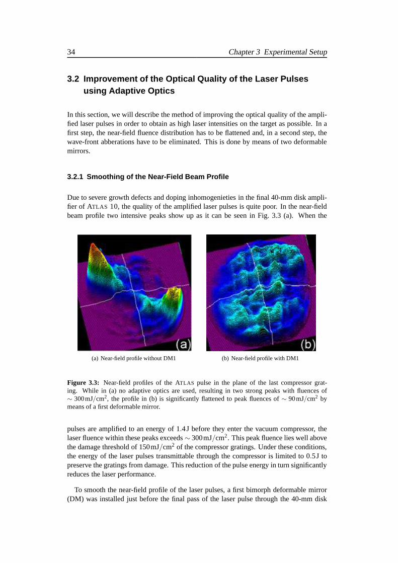
34 Chapter 3 Experimental Setup
3.2 Improvement of the Optical Quality of the Laser Pulsesusing Adaptive Optics
In this section, we will describe the method of improving theoptical quality of the ampli-fied laser pulses in order to obtain as high laser intensitieson the target as possible. In afirst step, the near-field fluence distribution has to be flattened and, in a second step, thewave-front abberations have to be eliminated. This is done by means of two deformablemirrors.
3.2.1 Smoothing of the Near-Field Beam Profile
Due to severe growth defects and doping inhomogenieties in the final 40-mm disk ampli-fier of ATLAS 10, the quality of the amplified laser pulses is quite poor. Inthe near-fieldbeam profile two intensive peaks show up as it can be seen in Fig. 3.3 (a). When the
(a) Near-field profile without DM1 (b) Near-field profile with DM1
Figure 3.3: Near-field profiles of the ATLAS pulse in the plane of the last compressor grat-ing. While in (a) no adaptive optics are used, resulting in two strong peaks with fluences of∼ 300mJ/cm2, the profile in (b) is significantly flattened to peak fluences of ∼ 90mJ/cm2 bymeans of a first deformable mirror.
pulses are amplified to an energy of 1.4J before they enter the vacuum compressor, thelaser fluence within these peaks exceeds∼ 300mJ/cm2. This peak fluence lies well abovethe damage threshold of 150mJ/cm2 of the compressor gratings. Under these conditions,the energy of the laser pulses transmittable through the compressor is limited to 0.5J topreserve the gratings from damage. This reduction of the pulse energy in turn significantlyreduces the laser performance.
To smooth the near-field profile of the laser pulses, a first bimorph deformable mirror(DM) was installed just before the final pass of the laser pulse through the 40-mm disk

3.2 Laser-Pulse Improvements by means of Adaptive Optics 35
amplifier, as it is sketched in Fig. 3.1. This first DM with a diameter of 30mm has 17active piezo electrodes. By applying voltages between−300V and+200V to the differentelectrodes, the surface of the mirror can be deformed locally. This changes the fluencedistribution in the near-field profile in a plane of the last compressor grating (which is≈ 11m downstream in the laser chain) and it can be controlled on-line by a CCD camera.As a result, the strong peaks in the beam profile are flattened and the profile is nearlytop-hat like as it is shown in Fig. 3.3 (b). With this fluence pattern, the laser pulses canenter the compressor with a maximal energy of up to 1.5J without damaging the gratings.
3.2.2 Correction of the Laser-Pulse Wave Front
On the other hand, the profile is flattened at the expense of additional wave-front distor-tions of the laser pulses leading to a very poor focusability. Fig. 3.4 shows the fluencedistribution in the focal plane as it is optained, when the first DM is optimised to give aflat beam profile as shown in Fig. 3.3 (b).
Figure 3.4: Fluence distribution of the laser pulses inthe focal plane of the off-axis parabolic mirror in the targetchamber. The first DM is optimised to obtain a smooth flu-ence pattern, but due to the strongly disturbed wave front,the focusability is quite poor and the pulse energy is scat-tered over a large area in the focal plane, resulting in lowpeak intensities.
To obtain laser pulses with a plane wave front and thus an improved focusability, thewave-front distortions have to be measured and then corrected in a controlled manner.This is done in the ATLAS laser by a closed-loop system consisting of a Shack-Hartmannsensor and a second computer-controlled DM. In the Shack-Hartmann sensor, the laserbeam passes through a 2-D array of small lenses. Each lens focuses a small local part ofthe beam onto a computer-read CCD resulting in a 2-D pattern of focal spots in the planeof the CCD chip. Any local wave-front distortion of the laserbeam causes a sideways shiftof the associated spot in the focal plane. After the focal-spot pattern of an expanded beamfrom a 790-nm laser diode of 75mm diameter with a wave-front distortion smaller thanλ/20 was taken as a reference pattern, the wave-front distortion of any other laser beamcan be quantified with this sensor by comparing its focal spotpattern with the pattern ofthe reference beam.
The wave-front abberations in the ATLAS pulses are corrected by a second DM locatedbehind the compressor in the evacuated tube system. This bimorph mirror of 80-mm di-ameter has 33 active piezo electrodes. The voltages appliedto each of these electrodes arecontrolled by the same computer, that is connected to the Shack-Hartmann sensor. First,the response of the wave front on changes in the voltage applied to each single electrode

36 Chapter 3 Experimental Setup
of the DM is determined. After that, the necessary voltages for all the electrodes to cor-rect the focal-spot pattern and therefore the wave front arecalculated by the computer andapplied to the second DM. In the next iteration, the corrected wave front is again mea-sured and compared to the reference. From this new difference, the new voltages for theDM are calculated. This iterative algorithm converges after three or four steps. Then theset of voltages is fixed and the flatness of the wave front, which is of the order ofλ/4,remains constant for hours within small shot-to-shot fluctuations of the laser. The drasticimprovement of the laser-pulse focusability is demonstrated in the next section.
As mentioned above, the near-field (NF) intensity distribution2 of ATLAS is not exactlytop-hat like but shows a less steep decay at the edges of the profile, as it is shown inFig. 3.3 (b). To quantitatively investigate the influence ofsuch a NF profile on the far-field (FF) intensity distribution, the NF profile was averaged within concentrical ringsgiving an averaged NF intensity distribution,INF(r), only depending on the radius,r. Theassociated electrical field distribution,ENF(r) ∝ [INF(r)]1/2, is shown by the red line inFig. 3.5 (a). For such a radially symmetric NF distribution,that can be described byENF(r), the FF distribution of the electrical field,EFF(ρ), is obtained from the followingintegration [97]
EFF(ρ) ∝1ρ2
w=∞∫
w=0
ENF(w) ·w ·J0(w)dw, (3.4)
wherew = 2πρr/ f λL is the normalised radius in the NF andJ0(w) is the Bessel func-tion (of the first kind) of order zero. This calculation only holds true for an ideally flatwave front. For a top-hat like profile, eq. (3.4) can be solvedanalytically and one obtainsthe Airy pattern. The NF distribution of ATLAS is shown in Fig. 3.5 (a) by the red linecompared both to a top-hat profile (black line) and a Super-Gaussian approximation of6th order (blue line). The FF distributions of the electric field for the three different NFprofiles are given in Fig. 3.5 (b). A weak dependence on the initial NF distribution isfound for the three cases. The radius of the first minimum differs from 2.5µm for thetop-hat profile to 2.6µm for the real profile. For the real ATLAS-profile a peak intensityin the center of the focal spot is found that is higher by a factor of ≈ 4.78 compared tothe intensity averaged over the area within the first minimum. A 2-D Fourier transfor-mation of the NF distribution carried out by R. Tommasini [98] gives the theoretical FFdistribution of the laser pulse, that is shown in Fig. 3.6. This distribution is not exactlyradially symmetric, as the NF profile also deviates from radial symmetry. However, theradii of the minima are well reproduced by the symmetrical approximation as depicted inFig. 3.5 (b).
From these considerations, we can conclude that a top-hat approximation for the NFdistribution of the ATLAS pulses is sufficient to derive the FF distribution and to calculatethe laser intensity.
2For the spatial distribution pulse intensity and fluence areequivalent, the latter is the first time-integratedover the pulse duration.

3.2 Laser-Pulse Improvements by means of Adaptive Optics 37
(a) Near-field intensity distributions (b) Far-field intensity distributions
Figure 3.5: Comparison of the radial electrical field distributions of the near-field of ATLAS (redline) with a top-hat like (black line) and a Super-Gaussian distribution of 6th order (blue line) in(a). (b) gives the corresponding radial distributions of the electrical field in the far field. The radiiof each first minimum in the far-field distributions differ between 2.5µm for the top-hat profileand 2.6µm for the real profile.
Figure 3.6: Theoretical far-field distributioncalculated from the ATLAS profile shown inFig. 3.3 (b) assuming a flat wave front.
3.2.3 Measurement of the Intensity Distribution in the Foca l Plane
For the measurement of a fluence distribution in the laser focus as they are shown inFigs. 3.4 and 3.7, the laser pulses were guided into the target chamber and focused by thef/2.6 off-axis parabolic mirror as in the real experiment. Ahigh-quality f/2−lens imagedthe focal plane with a magnification of∼ 50 onto an 8-bit CCD. To increase the dynamicalrange of this measurement, differently filtered images of the focus were subsequentlytaken. After these measurements, the images were added, taking into account the differentfilter transmissions and thereby increasing the dynamical range of the measurement tomore than 12 bits.
As on the one hand the imaging lens cannot sustain the high fluences occuring with the
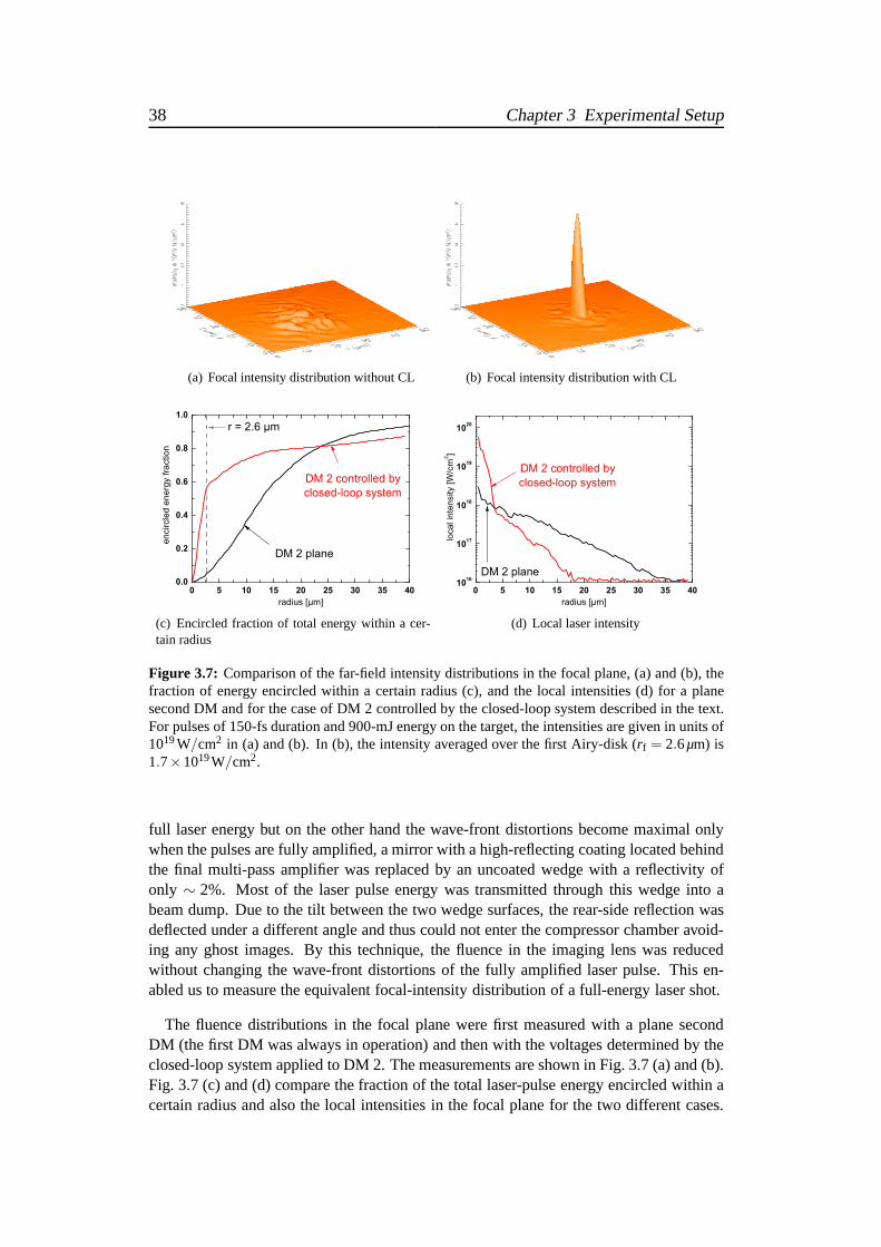
38 Chapter 3 Experimental Setup
(a) Focal intensity distribution without CL (b) Focal intensity distribution with CL
(c) Encircled fraction of total energy within a cer-tain radius
(d) Local laser intensity
Figure 3.7: Comparison of the far-field intensity distributions in the focal plane, (a) and (b), thefraction of energy encircled within a certain radius (c), and the local intensities (d) for a planesecond DM and for the case of DM 2 controlled by the closed-loop system described in the text.For pulses of 150-fs duration and 900-mJ energy on the target, the intensities are given in units of1019W/cm2 in (a) and (b). In (b), the intensity averaged over the first Airy-disk (rf = 2.6µm) is1.7×1019W/cm2.
full laser energy but on the other hand the wave-front distortions become maximal onlywhen the pulses are fully amplified, a mirror with a high-reflecting coating located behindthe final multi-pass amplifier was replaced by an uncoated wedge with a reflectivity ofonly ∼ 2%. Most of the laser pulse energy was transmitted through this wedge into abeam dump. Due to the tilt between the two wedge surfaces, therear-side reflection wasdeflected under a different angle and thus could not enter thecompressor chamber avoid-ing any ghost images. By this technique, the fluence in the imaging lens was reducedwithout changing the wave-front distortions of the fully amplified laser pulse. This en-abled us to measure the equivalent focal-intensity distribution of a full-energy laser shot.
The fluence distributions in the focal plane were first measured with a plane secondDM (the first DM was always in operation) and then with the voltages determined by theclosed-loop system applied to DM 2. The measurements are shown in Fig. 3.7 (a) and (b).Fig. 3.7 (c) and (d) compare the fraction of the total laser-pulse energy encircled within acertain radius and also the local intensities in the focal plane for the two different cases.
3.3 Control and Characterisation of the ASE Pedestal 39
While in (a), the laser-pulse energy is scattered over a large area resulting in several smallpeaks with low intensities, the energy in (b) is concentrated within a single narrow peakhaving only a weak low-intensity halo around it. The fraction of laser energy encirceledwithin a spot of 2.6-µm radius, which corresponds to the first Airy-disk in the focal plane3,is increased from∼ 5.5% in (a) to∼ 60% in (b), the peak intensity is increased by a factorof ∼ 20 to a peak value approaching 6×10¹⁹W/cm2 and an intensity averaged over thefirst Airy-disk of 1.7×10¹⁹W/cm2. The measured peak value gives a Strehl-ratio4 of∼ 0.7. The corresponding averaged intensity for the case of a second DM corrected tobe plane is only 1.6×10¹⁸W/cm2. Note that all these intensities correspond to normalincidence of the laser pulse onto the target. They are reduced for oblique incidence underthe angleα by a factor of cosα.
3.3 Control and Characterisation of the ASE Pedestal
In present CPA-laser systems as ATLAS, amplified spontaneous emission (ASE) fromthe pumped amplification crystals generates a low-intensity prepulse pedestal underneaththe short high-intensity pulse. The main contribution to this pedestal originates in theoscillator and the regenerative amplifier, and it is furtheramplified in the laser chain.Usually extending over several ns, the ASE pedestal is incoherent and passes the gratingcompressor unchanged typically resulting in an on-target intensity ratio of the order of107 between main pulse and prepulse pedestal. When the main pulse is focused ontothe target to intensities in excess of 1019W/cm2, the pedestal reaches an intensity of theorder of 1012. . .1013W/cm2 on a time scale of several ns preceding the peak intensity.This is sufficient to preheat and ionise the surface of a solidtarget producing an expandedplasma on the target-front side. In addition, a shock wave islaunched by the ASE prepulsethat propagates through the target, preheats the bulk of thematerial and – especially withthin foils – destroys the target before the main pulse arrives at the surface, what is highlyunwanted. We will concentrate on this fact and its consequences for experiments in a laterchapter. Therefore, the characterisation of the prepulse pedestal is of great importancefor precise laser-plasma experiments. Intensity and especially the duration of the ASEprepulse have to be known or – even better – controlled as accurately as possible.
Within the framework of this thesis, the characterisation and controllability of the pre-pulse pedestal in ATLAS was significantly enhanced by implementing an additional ultra-fast Pockels cell into the laser chain. This enabled us for the first time to do systematicstudies of prepulse dependent effects on the acceleration of protons and ions from thinfoils [47]. While the results from these measurements will be presented in chapter 5, wewill describe the setup of the Pockels cell and demonstrate its effect on the ASE pedestalin the next sections.
3Here we used the far-field distribution associated to the real near-field profile of ATLAS.4The Strehl-ratio is defined as the ratio between real peak intensity and theoretical peak intensity, which is
4.78-times higher than the averaged intensity as we have shown above.
40 Chapter 3 Experimental Setup
3.3.1 Pockels Cells used as Optical Shutters
To reduce the intensity and duration of the pedestal preceding the main pulse, appro-priately gated Pockels cell (PC) shutters are used in the laser chain. A PC contains anuniaxial electro-optical crystal (e.g. Potassium di-Hydrogen Phosphate, KDP) with theoptical axis aligned along the direction of laser propagation. It becomes an optically bi-axial crystal, when an external voltage is applied along theoptical axis. For a certainvoltage,Uλ/2 of the order of 5kV, the crystal acts like aλ/2-wave plate for the wavelengthλ, rotating the plane of polarisation of the incident light wave by 90. If the PCis positioned between two crossed polarisers, it can be usedas an optical shutter. Theincoming light wave passes the first polariser (e.g. a Glan prism) and the PC. It is blockedby the second polariser when no voltage is applied to the PC, but it can pass when thevoltage matchesUλ/2. In a laser system,Uλ/2 is applied by means of a high-voltage (HV)pulser just before the arrival of the main pulse. The preceding ASE pedestal is blockedand only the main pulse can pass, as its polarisation is rotated by the PC. Nevertheless,the minimal duration of the pedestal preceding the main pulse is limited by the followingfactors:
• The optical shutter has to be opened completely before the main pulse passesthrough to avoid its clipping. Therefore, theelectronicrise time of the HV signalapplied to the crystal is a lower limit for the minimal duration of the ASE pedestal.
• Theoptical rise time of the PC scales with the diameter of the electro-optical crys-tal, additionally increasing thetotal opening time of the optical shutter.
• As the PC is located at a position in the laser chain, where themain pulse is stillstretched to∼150ps to avoid optical damages in the material, the pedestalwithinthis time window cannot be reduced without clipping a part the main pulse. Afterrecompression, which leaves the incoherent pedestal unchanged, the main pulse sitsin the middle of this pedestal, which then starts∼75ps before the peak intensity.
• The suppression factor of a single PC is limited to∼ 500. . .1000 due to non-idealpolarisation and parallelism of the incoming laser beam.
3.3.2 System of Pockels Cells in ATLAS
In ATLAS two PCs are used to control the ASE pedestal preceding the main pulse. Thesetup is sketched in Fig. 3.8. While PC 3 is controlled by a slow HV pulser having asignal-rise time of∼5. . .6ns, an ultra-fast HV pulser (KENTECHPulse Generator GPS3/S[99]) is used for PC 4. It delivers a rectangular HV signal with a rise time of∼120ps anda duration of 5ns. The total rise time of the optical gate is increased to∼250. . .300ps dueto the finite diameter and response time of the PC, the duration of the gate is increasedto 6ns. Due to the jitter of the electronic trigger for the KENTECH pulser (τjitter∼150ps),the duration of the pedestal was chosen to be longer byτjitter to avoid clipping of themain pulse at the expense of shortening the prepulse. After recompression, the minimumachievable duration of the ASE pedestal at an intensity level of ∼1012W/cm2 on the target
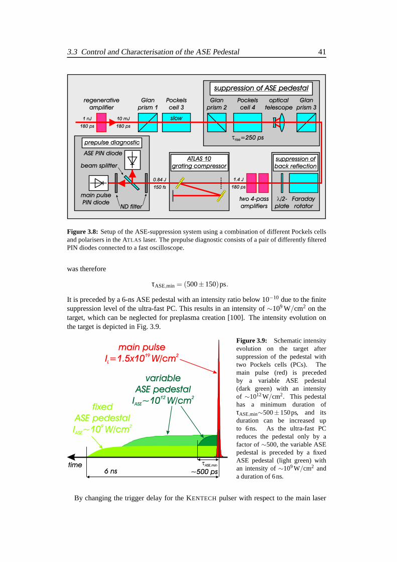
3.3 Control and Characterisation of the ASE Pedestal 41
Pockels
cell 3
Glan
prism 1
Glan
prism 2
trise=250 ps
Pockels
cell 4
Faraday
rotator
slow
suppression of ASE pedestal
0.84 J
150 fs
optical
telescope
Glan
prism 3
l/2-
plate
two 4-pass
amplifiers
regenerative
amplifier
suppression of
back reflection
1.4 J
180 ps
10 mJ
180 ps
1 nJ
180 ps
ND filter
ASE PIN diode
main pulse
PIN diode
ATLAS 10
grating compressor
prepulse diagnostic
beam splitter
Figure 3.8: Setup of the ASE-suppression system using a combination of different Pockels cellsand polarisers in the ATLAS laser. The prepulse diagnostic consists of a pair of differently filteredPIN diodes connected to a fast oscilloscope.
was therefore
τASE,min = (500±150)ps.
It is preceded by a 6-ns ASE pedestal with an intensity ratio below 10−10 due to the finitesuppression level of the ultra-fast PC. This results in an intensity of∼109 W/cm2 on thetarget, which can be neglected for preplasma creation [100]. The intensity evolution onthe target is depicted in Fig. 3.9.
main pulse
I =1.5x10 W/cmL
19 2
variable
ASE pedestal
I ~10 W/cmASE
12 2
fixed
ASE pedestal
I ~10 W/cmASE
9 2
time6 ns
tASE,min
~500 ps
Figure 3.9: Schematic intensityevolution on the target aftersuppression of the pedestal withtwo Pockels cells (PCs). Themain pulse (red) is precededby a variable ASE pedestal(dark green) with an intensityof ∼1012W/cm2. This pedestalhas a minimum duration ofτASE,min∼500±150ps, and itsduration can be increased upto 6ns. As the ultra-fast PCreduces the pedestal only by afactor of∼500, the variable ASEpedestal is preceded by a fixedASE pedestal (light green) withan intensity of∼109W/cm2 anda duration of 6ns.
By changing the trigger delay for the KENTECH pulser with respect to the main laser
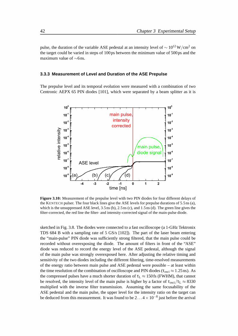
42 Chapter 3 Experimental Setup
pulse, the duration of the variable ASE pedestal at an intensity level of∼ 1012W/cm2 onthe target could be varied in steps of 100ps between the minimum value of 500ps and themaximum value of∼6ns.
3.3.3 Measurement of Level and Duration of the ASE Prepulse
The prepulse level and its temporal evolution were measuredwith a combination of twoCentronic AEPX 65 PIN diodes [101], which were separated by abeam splitter as it is
Figure 3.10: Measurement of the prepulse level with two PIN diodes for four different delays ofthe KENTECHpulser. The four black lines give the ASE levels for prepulsedurations of 5.5ns (a),which is the unsuppressed ASE level, 3.5ns (b), 2.5ns (c), and 1.5ns (d). The green line gives thefilter-corrected, the red line the filter- and intensity-corrected signal of the main-pulse diode.
sketched in Fig. 3.8. The diodes were connected to a fast oscilloscope (a 1-GHz TektronixTDS 684 B with a sampling rate of 5 GS/s [102]). The part of the laser beam enteringthe “main-pulse” PIN diode was sufficiently strong filtered,that the main pulse could berecorded without overexposing the diode. The amount of filters in front of the “ASE”diode was reduced to record the energy level of the ASE pedestal, although the signalof the main pulse was strongly overexposed here. After adjusting the relative timing andsensitivity of the two diodes including the different filtering, time-resolved measurementsof the energy ratio between main pulse and ASE pedestal were possible – at least withinthe time resolution of the combination of oscilloscope and PIN diodes (τosci≈ 1.25ns). Asthe compressed pulses have a much shorter duration ofτL ≈ 150fs (FWHM), that cannotbe resolved, the intensity level of the main pulse is higher by a factor ofτosci/τL ≈ 8330multiplied with the inverse filter transmission. Assuming the same focusability of theASE pedestal and the main pulse, the upper level for the intensity ratio on the target canbe deduced from this measurement. It was found to be 2. . .4×10−8 just before the arrival

3.3 Control and Characterisation of the ASE Pedestal 43
of the main pulse. Results from the measurement are shown in Fig. 3.10.
As the rise time of the ASE pedestal was expected to be much shorter (∼ 300. . .500ps)than the time resolution of the 1-GHz oscilloscope and the Centronic PIN diodes, wecarried out a separate measurement with a 4-GHz oscilloscope (Tektronix CSA 7404 B[102]) having a sample rate of 20GS/s and an extremely fast GaAs-PIN diode (ET-4000[103]) together having a time resolution of∼ 130ps. In this measurement, the time-resolved increase of the prepulse intensity could be recorded, and the results are shown inFig. 3.11.
Figure 3.11: Temporal evolution of the ASE prepulse measured with a 4-GHzoscilloscope and aGaAs-PIN diode with four different trigger delays for the ultra-fast Pockels cell. The green linegives the unsuppressed ASE, the other three lines give the measured (solid) ASE evolutions forprepulse durations ofτASE = 2.5ns (blue), 1.0ns (red), and 0.5ns (black), respectively. The mainpulse starts att = 0.
For the shortest prepulse duration ofτASE = 500ps (solid black line), the rise time of theASE pedestal is also on the order of 500ps. The rise time appears to increase for longerprepulse durations, but the changes are only marginal. After the linear increase of theASE intensity, it remains constant at an intensity level of(2. . .4)×10−8 until the arrivalof the main pulse increases the intensity by several orders of magnitude. For a prepulseduration of 2.5ns (blue line), the rise time is increased to∼ 1.0ns, as the unsuppressedASE level (green line) is also not constant.
Taking the results of these two measurements together, we could exactly characterisethe temporal evolution of the ASE prepulse. The maximum ASE level is(2. . .4)×10−8.The prepulse duration could be controlled by changing the trigger delay for the ultra-fast

44 Chapter 3 Experimental Setup
PC. The rise-times for different trigger delays could be resolved and are approximatelylinear. This measurement allows an exact numerical modeling of the preplasma formationon both target surfaces. The corresponding simulations will be presented in chapter 6.
Chapter 4
Detection of Laser-Accelerated Protons andLight Ions in the Experiment
This chapter describes the diagnostics used in the experiments to characterise the ionbeam formed during the interaction of the high-intensity laser pulse from ATLAS 10 witha thin foil. Three different diagnostics were employed:
1. the plastic nuclear track detector CR 39,
2. a time-of-flight (TOF) detector coupled to a fast oscilloscope, and
3. a Thomson parabola magnetic spectrometer.
These three different types of detectors will now be described in detail.
4.1 Ion Detection with CR 39 Nuclear Track Detectors
Preliminary measurements using a simple setup were performed to show that protons canbe accelerated to MeV-energies in thin-foil experiments using the ATLAS 10 laser. Forthat purpose pieces of CR 39 were used to detect the protons. CR 39 is a solid state nucleartrack detector fabricated of polymeric plastic. The piecesof CR 39 used in this thesis wereproduced by TASL in Bristol, UK [104]. When an energetic particle propagates throughthe plastic, it deposits certain amounts of its kinetic energy along its path in the materialdepending on the particle’s cross-section and its momentary energy while it is deceleratedand finally stopped. If the amount of locally deposited energy exceeds a certain threshold,the polymeric chains of the detector material break up at this position. Thus the energeticparticle leaves a trace along its path in the material until it is stopped. As the cross-sectionsfor electrons andγ-rays are much lower than that for ions, and as the locally depositedenergy therefore remains below the threshold for chain break-up1, the detector is sensitiveto ion impacts only. Furthermore, protons with kinetic energies between 100keV and5MeV leave significant traces at the front surface of the detector material, where they can
1This holds true as long as the flux of electrons andγ-rays is not too high. In the experiments reported onin this thesis, no detectable effect of electrons orγ-rays on CR 39 could be observed, as the fluxes weretoo low.
45

46 Chapter 4 Proton and Ion Diagnostics
be detected afterwards. This predestines CR 39 as an ideal ion detector in laser-plasmaexperiments, as also very small ion signals can be detected within the “noise” generatedby any other energetic radiation occurring in high-intensity interactions.
The most common way to make the ion hits visible is to etch the plastic in hot NaOHsolution [105]. As the etching rates of the plastic differ between regions with undisturbedpolymeric structure and regions where an ion broke up the polymeric chains, while it lostpart of its kinetic energy, small pits on the scale of severalµm are formed on the surfaceof the CR 39 plastic. These pits can easily be detected under an optical microscope [82].
Figure 4.1: Setup for the preliminary detectionof protons using CR 39 plates partly wrapped with a15-µm aluminum foil standing∼9cm behind the target.The minimum kinetic energies for the protons that canbe detected by the two parts of the detector are 1MeVand 100keV for the wrapped and unwrapped part of thedetector, respectively.
targetelectrons
ions
ATLAS 10 beam
I =1.5x10 W/cmL
19 2
30°
CR 39 detector
15 µm Al
The experimental setup for the preliminary proton detection is shown in Fig. 4.1. TheCR 39 plates were positioned∼9cm behind the target around its normal direction. Onepart of the CR 39 was covered with a 15-µm aluminum foil, the other part remained un-shielded providing a detector sensitive to protons with twodifferent minimum energies.Using the CSDA stopping ranges of protons in aluminum published by the National Insti-tute of Standards and Technology (NIST, [106]), the stopping ranges,d, for protons withkinetic energies,Ekin, between 300keV and 4MeV can be approximated by
d ≈ 16µm× (Ekin/1MeV)1.45. (4.1)
Thus the minimum proton energies detected by the CR 39 are 1MeV and 100keV for theshielded and unshielded part of the detector, respectively. The minimum proton energydetectable by bare CR 39 is determined by the threshold that has to be overcome to causesignificant damage in the polymeric structure of the detector material.
Figure 4.2: Magnified picture ofa CR 39 plate after etching. Theleft part was unshielded, the rightpart was covered with a 15-µm alu-minum foil. While the left part issaturated with pits from ions withkinetic energies above 100keV, inthe right part single pits of 1. . .2µmdiameter can be distinguished.
50 µm

4.2 Time-Of-Flight Detector 47
A magnified section of a piece of CR 39 is shown in Fig. 4.2. The plate has been etchedfor 2 hours in 6-molar NaOH solution at∼80C. We show the boundary between the twodifferently shielded parts of the detector. The left side was unshielded and thus sensitiveto any ion with a kinetic energy above 100keV, the right side was wrapped with a 15-µmaluminum foil. In this part, single pits can be distinguished. They can only originate fromprotons with kinetic energies exceeding 1MeV.
After this first experimental proof of the acceleration of MeV-protons with the ATLASlaser, a more precise diagnostic was needed to characterisethe proton beam and its energyspectrum. For this purpose, we used a time-of-flight detector described in the next section.
4.2 Spectral Characterisation of the Ion Beam using aTime-Of-Flight Detector
4.2.1 Setup of the Detector
A time-of-flight (TOF) detector realised as a Faraday cup [107], as it is depicted inFig. 4.3, is sensitive to the total electric current,I(tTOF), impinging at timetTOF on thecharge collector of the detector. The temporal evolution ofthe current can be recorded
R = 1 MW
U = -1.0 kVC U = -1.1 kVB
charge
collector
Ni-mesh (55-µm apertures)
secondary
electron
suppression
C = 1 µF
to fast
oscilloscope
(50 )W ions
electrons
Figure 4.3:Schematic diagram ofan ion TOF detectorincluding a meshto shield the chargecollector against co-propagating electronsand a metallic cylinderto suppress the effectof secondary electronsgenerated at the chargecollector.
by means of an ultra-fast oscilloscope connected to the detector. As the detector is stand-ing at a defined distance,dTOF, from the target, where the ions are generated, the ions aretemporally dispersed due to their different velocities,vi , or kinetic energies,Ekin. If theflying time of the ions,tTOF, is much longer than the time interval within which they aregenerated2, we find a direct relation betweenEkin andtTOF:
Ekin =mi
2·vi
2 =mi ·d2
TOF
2· t−2
TOF, (4.2)
wheremi is the ion mass. As the maximum kinetic energies of the ions measured inthe experiments are well below their rest mass (for protons with rest massmp we obtainEmax∼ 5MeV mpc2 = 938MeV), the classical treatment is sufficient.
2The flying time of the ions for our detector setup is of the order of 10ns and longer, as it will be shownbelow, while the generation time is of the order of the laser pulse duration,τL = 150fs.
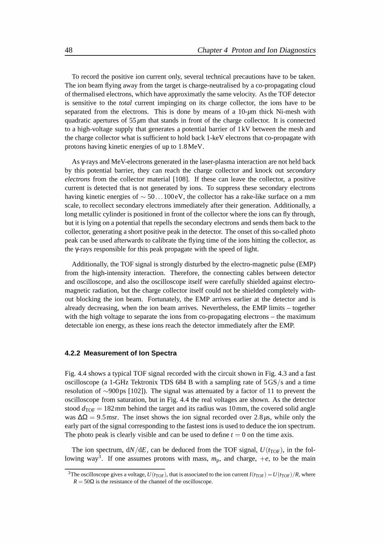
48 Chapter 4 Proton and Ion Diagnostics
To record the positive ion current only, several technical precautions have to be taken.The ion beam flying away from the target is charge-neutralised by a co-propagating cloudof thermalised electrons, which have approximatly the samevelocity. As the TOF detectoris sensitive to thetotal current impinging on its charge collector, the ions have to beseparated from the electrons. This is done by means of a 10-µm thick Ni-mesh withquadratic apertures of 55µm that stands in front of the charge collector. It is connectedto a high-voltage supply that generates a potential barrierof 1kV between the mesh andthe charge collector what is sufficient to hold back 1-keV electrons that co-propagate withprotons having kinetic energies of up to 1.8MeV.
As γ-rays and MeV-electrons generated in the laser-plasma interaction are not held backby this potential barrier, they can reach the charge collector and knock outsecondaryelectronsfrom the collector material [108]. If these can leave the collector, a positivecurrent is detected that is not generated by ions. To suppress these secondary electronshaving kinetic energies of∼ 50. . .100eV, the collector has a rake-like surface on a mmscale, to recollect secondary electrons immediately aftertheir generation. Additionally, along metallic cylinder is positioned in front of the collector where the ions can fly through,but it is lying on a potential that repells the secondary electrons and sends them back to thecollector, generating a short positive peak in the detector. The onset of this so-called photopeak can be used afterwards to calibrate the flying time of theions hitting the collector, astheγ-rays responsible for this peak propagate with the speed of light.
Additionally, the TOF signal is strongly disturbed by the electro-magnetic pulse (EMP)from the high-intensity interaction. Therefore, the connecting cables between detectorand oscilloscope, and also the oscilloscope itself were carefully shielded against electro-magnetic radiation, but the charge collector itself could not be shielded completely with-out blocking the ion beam. Fortunately, the EMP arrives earlier at the detector and isalready decreasing, when the ion beam arrives. Nevertheless, the EMP limits – togetherwith the high voltage to separate the ions from co-propagating electrons – the maximumdetectable ion energy, as these ions reach the detector immediately after the EMP.
4.2.2 Measurement of Ion Spectra
Fig. 4.4 shows a typical TOF signal recorded with the circuitshown in Fig. 4.3 and a fastoscilloscope (a 1-GHz Tektronix TDS 684 B with a sampling rate of 5GS/s and a timeresolution of∼900ps [102]). The signal was attenuated by a factor of 11 to prevent theoscilloscope from saturation, but in Fig. 4.4 the real voltages are shown. As the detectorstooddTOF = 182mm behind the target and its radius was 10mm, the covered solid anglewas∆Ω = 9.5msr. The inset shows the ion signal recorded over 2.8µs, while only theearly part of the signal corresponding to the fastest ions isused to deduce the ion spectrum.The photo peak is clearly visible and can be used to definet = 0 on the time axis.
The ion spectrum, dN/dE, can be deduced from the TOF signal,U(tTOF), in the fol-lowing way3. If one assumes protons with mass,mp, and charge,+e, to be the main
3The oscilloscope gives a voltage,U(tTOF), that is associated to the ion currentI(tTOF) =U(tTOF)/R, whereR= 50Ω is the resistance of the channel of the oscilloscope.

4.2 Time-Of-Flight Detector 49
Figure 4.4: Ion TOF signal,U(t), obtained with a 8-µm Mylar foil. The early part of the signalis zoomed in from the total time window of 2.8µs given in the inset. The red line gives the signalafter applying a low-pass filter to reduce the EMP-noise. This filtered signal is used to deduce theion spectrum (see text). The onset of the photo peak definest = 0. The indicated arrival timeshold for protons with kinetic energies of 1MeV, 500keV, and 100keV. The signal extending overseveralµs in the inset is associated with the plasma blow-off.
contribution to this ion signal (carbon and oxygen ions can only be distinguished with aThomson parabola, what will be discussed later), one obtains with help of eq. (4.2)
∣
∣
∣
∣
dNdE
∣
∣
∣
∣
=dNdt
·∣
∣
∣
∣
dtdE
∣
∣
∣
∣
=Iprot(tTOF)
q·∣
∣
∣
∣
dtdE
∣
∣
∣
∣
=1e
U(tTOF)
R· dTOF
2
√
mp
2E(tTOF)3 =
=1
e·mp· 1
d2TOF ·R
·U(tTOF) · t3TOF, (4.3)
where Iprot(tTOF) is the proton current impinging on the charge collector,R = 50Ω isthe resistance of the channel of the fast-oscilloscope, andU(tTOF) is the voltage detectedby the oscilloscope. Using this expression, the proton spectrum is easily obtained. Thespectrum per solid angle corresponding to the TOF signal in Fig. 4.4 is shown in Fig. 4.5.
In this spectrum, protons with kinetic energies up to 1.5MeV are detected. The spec-trum shows two distinct proton populations, one with a Boltzmann-like temperature ofTcold = 65keV and a second one withThot = 200keV.
The spectrum in Fig. 4.5 was deduced assuming protons being the only ion speciesin the detected beam. Any additional ion species (e.g. carbon or oxygen) would alsoaffect the spectrum, especially for higher charge states. If one assumes that carbon ionswith the same kinetic energy as the protons, i.e.Ekin = 1.5MeV, are also acceleratedfrom the target, they have a velocity smaller by a factor of 1/
√12 due to their higher
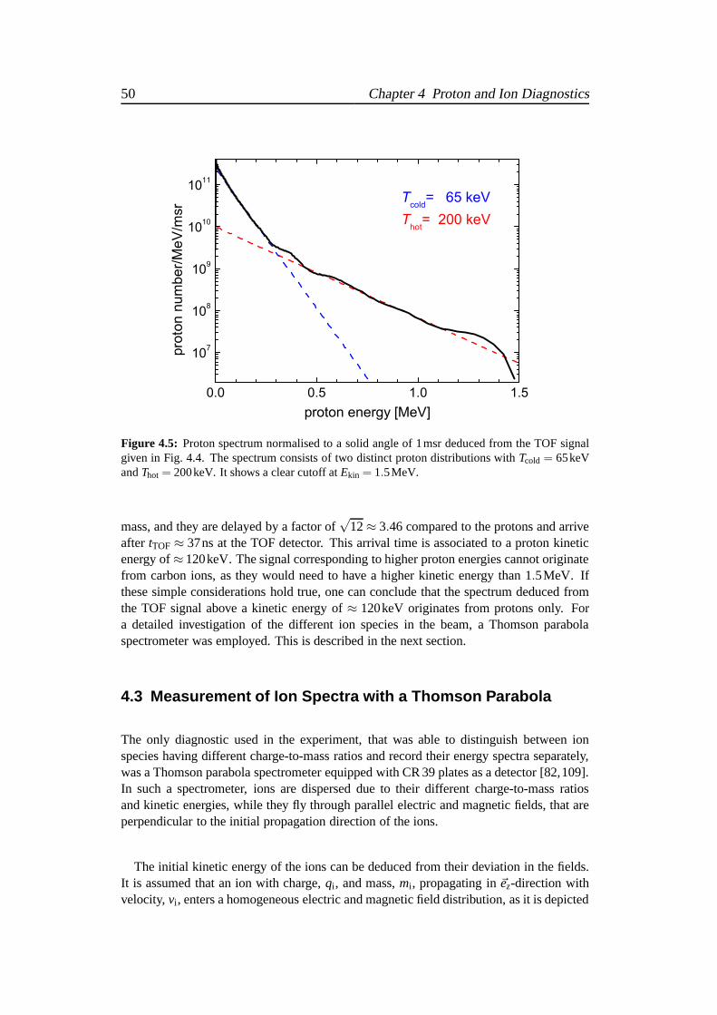
50 Chapter 4 Proton and Ion Diagnostics
Figure 4.5: Proton spectrum normalised to a solid angle of 1msr deduced from the TOF signalgiven in Fig. 4.4. The spectrum consists of two distinct proton distributions withTcold = 65keVandThot = 200keV. It shows a clear cutoff atEkin = 1.5MeV.
mass, and they are delayed by a factor of√
12≈ 3.46 compared to the protons and arriveafter tTOF ≈ 37ns at the TOF detector. This arrival time is associated to aproton kineticenergy of≈ 120keV. The signal corresponding to higher proton energiescannot originatefrom carbon ions, as they would need to have a higher kinetic energy than 1.5MeV. Ifthese simple considerations hold true, one can conclude that the spectrum deduced fromthe TOF signal above a kinetic energy of≈ 120keV originates from protons only. Fora detailed investigation of the different ion species in thebeam, a Thomson parabolaspectrometer was employed. This is described in the next section.
4.3 Measurement of Ion Spectra with a Thomson Parabola
The only diagnostic used in the experiment, that was able to distinguish between ionspecies having different charge-to-mass ratios and recordtheir energy spectra separately,was a Thomson parabola spectrometer equipped with CR 39 plates as a detector [82,109].In such a spectrometer, ions are dispersed due to their different charge-to-mass ratiosand kinetic energies, while they fly through parallel electric and magnetic fields, that areperpendicular to the initial propagation direction of the ions.
The initial kinetic energy of the ions can be deduced from their deviation in the fields.It is assumed that an ion with charge,qi , and mass,mi, propagating in~ez-direction withvelocity,vi , enters a homogeneous electric and magnetic field distribution, as it is depicted

4.3 Thomson Parabola 51
electrodes
BE
magnets
DX
DY
ez
ey
ex
pinhole
zD origin
Figure 4.6: Schematic layout of a Thomson parabola. Ions coming from thetarget pass througha small pinhole and fly through parallel electric and magnetic fields generated by two pairs ofelectrodes and magnets. In these fields, they are dispersed onto distict parabola traces in the planeof the detector. In this sketch, only ions of the same speciesbut with different velocities are shown.
in Fig. 4.6. The field lines are parallel to~ex. After the ion has moved through the fielddistribution in~ez-direction, it has been deflected sideways by the fields. If one assumes aconstant field strength over the total extension,z, of the fields and neglects fringe effects,the deflection parallel to~ex due to the electric field,E , is for small deviations given by
∆x∼ 12
at2 =Ez2
2· qi
mivi2 , (4.4)
which is inversely proportional to the ion kinetic energy,Ekin = mivi2/2. The deflection
in ~ey-direction due to the magnetic field,B , can be written as
∆y∼ 12
at2 =Bz2
2· qi
mivi(4.5)
and is thus inversely proportional to the momentum,pi = mivi , of the ion. Here we as-sume a constant velocity,vi , when the ion passes through the fields, although it is slightlyincreased by the electric field. When the ion hits the detector which is positioned in dis-tance,D, from the center of the fields, the total deviations are then given by
∆X ∼ EDz· qi
mivi2 and ∆Y ∼ BDz· qi
mivi. (4.6)
Taking these two equations together,∆X can be written as
∆X ∼ E
B2Dz· mi
qi· (∆Y)2, (4.7)
which is a parabolic equation with the inverse charge-to-mass ratio as a parameter. Notethat the deflection along a single parabola trace in the planeof the detector depends on

52 Chapter 4 Proton and Ion Diagnostics
the ion velocity, but different ion species lie on parabolaswith different slopes. The ionspecies with the highest charge-to-mass ratio (in our experiments protons withqi/mi =1·e/u) forms the parabola trace, which is least bent in~ex-direction.
Figure 4.7: Digital photographof a CR 39 plate after etching. Theleft side shows the bare detectorwith parabola traces from seven dif-ferent ion species. The origin ofthe parabolas is formed by neu-tral atoms that pass through theThomson parabola unaffected bythe fields. On the right side, thetraces obtained by a 3-D trackingroutine are compared to the mea-sured traces. A very good agree-ment is found that allows a clear de-termination of the ion species.
p+
C3+
C1+
C5+
C2+
O6+
C4+
origin origin
Fig. 4.7 shows a piece of CR 39, that has been etched in hot NaOHsolution after asingle laser shot. Seven different parabola traces are visible. The origin of all tracesin the lower right corner is generated by ions that have recombined with co-propagatingelectrons before entering the spectrometer. As they are electrically neutral, they are notdeflected by the fields and form a spot on the detector which would also correspond to acharged ion with infinite velocity.
To identify the ion species with a certain charge-to-mass ratio forming a single parabolatrace, a 3-D tracking routine for different ion species and different velocities through thereal electric and magnetic fields was carried out by J. Schreiber [110]. The magnetic fielddistribution was measured with a Hall-sensor, the electricfield distribution and the iontrajectories through the fields were simulated using the program EM STUDIOTM [111].The excellent agreement between the calculated and measured traces, as it can be seenin the right part of Fig. 4.7, allows a definite assignment of the different traces on thedetector to protons, C1+ to C5+, and O6+ ions.
Each parabola trace consists of a large number of ion pits. They can be separated underan optical microscope, as it is shown in Fig. 4.8. The microscope having ax−y translationstage and a connected CCD are controlled by a computer. A pattern-recognition softwarefits ellipses to the pits and stores their diameters and positions. Starting from the originon the detector, the deviations of the charged ions can be measured easily. With thedispersion relations obtained by the tracking routine, theenergy spectra of the differention species can be deduced from the stored deviations of the ion pits. The energy spectrafor the protons and the different Carbon-species deduced from the CR 39 plate shown inFig. 4.7 are presented in Fig. 4.9.

4.3 Thomson Parabola 53
Figure 4.8: Magnified part of theproton parabola trace on a piece ofCR 39 after etching. The green el-lipses were fitted to the proton pitsby the computer software. Their po-sitions and diameters are stored forsubsequent spectral analysis. Evenslightly overlapping pits can be re-solved. The fitting of pits essen-tially smaller than the proton pits(e.g. from dust) is either suppressed,or the ellipses can be excluded af-terwards due to their smaller diam-eters.
Figure 4.9: Proton and carbon spectra corresponding to the CR 39 plate shown in Fig. 4.7.
Different Methods for Deduction of Ion-Energy Spectra
To obtain an energy spectrum, dN(E)/dE ≈ ∆N(E)/∆E, of a certain ion species, thenumber of ions,∆N(E), within the energy interval,[E,E + ∆E], has to be determined. Inthe plane of the CR 39 detector, the ion pits are spread according to their kinetic energy,E, on a parabola trace. An energy interval,[E,E+∆E], corresponds to an interval,[y,y+∆y], along the~ey−axis deviation on the detector, described by the ion-dispersion relation,dE/dy. ∆N(E) can either be taken within aconstant energy interval, ∆E, or within aconstant deviation interval, ∆y, over the whole parabola trace. In the first case of constant∆E, the corresponding∆y(E)-interval becomes smaller, in the second case of constant∆y,the energy interval,∆E(E), becomes larger for increasing ion energy,E. As ions havingexactly the same kinetic energy are scattered within the parabola trace at least over an area
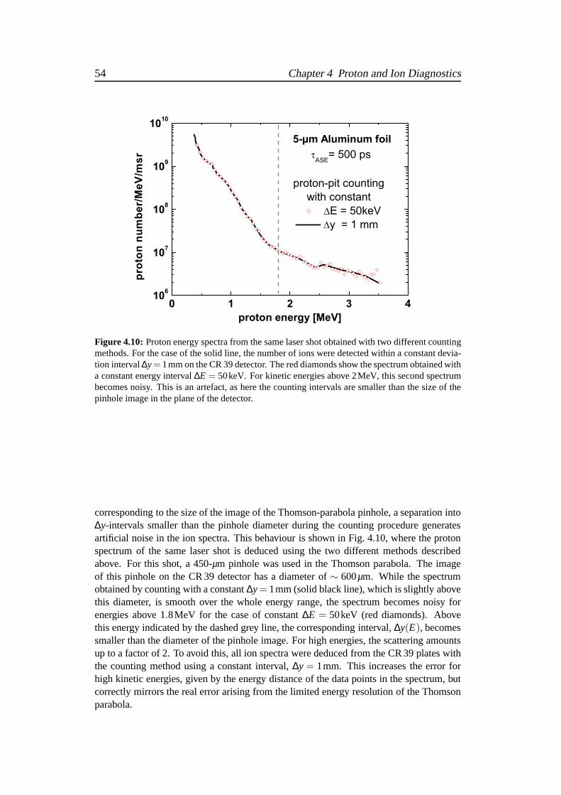
54 Chapter 4 Proton and Ion Diagnostics
Figure 4.10: Proton energy spectra from the same laser shot obtained withtwo different countingmethods. For the case of the solid line, the number of ions were detected within a constant devia-tion interval∆y= 1mm on the CR 39 detector. The red diamonds show the spectrum obtained witha constant energy interval∆E = 50keV. For kinetic energies above 2MeV, this second spectrumbecomes noisy. This is an artefact, as here the counting intervals are smaller than the size of thepinhole image in the plane of the detector.
corresponding to the size of the image of the Thomson-parabola pinhole, a separation into∆y-intervals smaller than the pinhole diameter during the counting procedure generatesartificial noise in the ion spectra. This behaviour is shown in Fig. 4.10, where the protonspectrum of the same laser shot is deduced using the two different methods describedabove. For this shot, a 450-µm pinhole was used in the Thomson parabola. The imageof this pinhole on the CR 39 detector has a diameter of∼ 600µm. While the spectrumobtained by counting with a constant∆y= 1mm (solid black line), which is slightly abovethis diameter, is smooth over the whole energy range, the spectrum becomes noisy forenergies above 1.8MeV for the case of constant∆E = 50keV (red diamonds). Abovethis energy indicated by the dashed grey line, the corresponding interval,∆y(E), becomessmaller than the diameter of the pinhole image. For high energies, the scattering amountsup to a factor of 2. To avoid this, all ion spectra were deducedfrom the CR 39 plates withthe counting method using a constant interval,∆y = 1mm. This increases the error forhigh kinetic energies, given by the energy distance of the data points in the spectrum, butcorrectly mirrors the real error arising from the limited energy resolution of the Thomsonparabola.

4.4 Spatial Profile of the Proton Beam 55
4.4 Measurement of the Spatial Profile of the Proton Beam
Finally, the spatial profile of the generated proton beam wasmeasured to have an estimateof the divergence of the beam. Both the energy spectrum and the profile of the protonbeam had to be measured from the same laser shot to eliminate shot-to-shot fluctuationson the one hand and to be able to valuate these fluctuations quantitatively on the otherhand. For this purpose, a piece of CR 39 was again positioned behind the target at adistance of 82mm. Its front side was completely wrapped witha 12-µm aluminum foil toblock protons with energies below 900keV. A part of the ion beam could pass througha small hole both in the detector and the aluminum foil to be detected in the Thomsonparabola simultaneously. Fig. 4.11 shows a typical spatialprofile of the proton beam, thatwas accelerated from a 5-µm aluminum foil. Around the target normal direction, indicatedby the small hole in the middle of the detector, a collimated proton feature appears thathas a half opening angle of∼10.
10° Figure 4.11: Spatial profile of the proton beamobtained with a 5-µm Al foil recorded on a pieceof CR 39. The dotted circle corresponds to a half-opening angle of 10. The main part of the protonbeam appears to be collimated around the targetnormal direction, indicated by the hole in the de-tector. Any pits on this CR 39 plate originate fromprotons with kinetic energies exceeding 900keV.The right part gives the line-out of the photo-graphic image along the dashed vertical line sug-gesting a ring-like beam profile (see text).
As the diameter of the hole was only 3.5mm, the alignment of this detector plate wascrucial to avoid any clipping of the ion beam along its path from the target to the Thomsonparabola. Therefore, a Helium-Neon laser was aligned through the pinhole of the Thom-son parabola pointing onto the target rear surface. This laser beam thus had the same pathas the ion beam coming from the target and entering the Thomson parabola through thepinhole. Before a shot with the main pulse, the hole of the CR 39 plate was positionedaround the Helium-Neon laser beam.
For the photograph shown in Fig. 4.11, the CR 39 piece was positioned in front of ablack screen and illuminated under oblique incidence from the back by a strong lampavoiding direct light from the lamp into the camera. From a region on the CR 39 coveredwith ion pits, light is scattered into the camera resulting in a bright region on the photo-graph. From regions with a plane surface, i.e. without ion pits, no light is scatterd intothe camera resulting in a dark region. On the photograph in Fig. 4.11, there appears to bea ring-like region with higher pit-densities (around the dashed circle), while the centralregion appears to be darker aggain suggesting a lower pit density here. The right partof Fig. 4.11 gives the line-out of the picture along the dashed vertial line illustrating thebrightness distribution that also suggests a ring-like beam profile. Such ring-like featureson CR 39 detectors have been observed in several experimentsand have been interpreted

56 Chapter 4 Proton and Ion Diagnostics
as signatures of a ring-like spatial profile of the proton beam caused by magnetic fieldsin the target [13, 14, 44] or at the rear surface of the target [46]. The combination of thetwo proton diagnostics (Thomson parabola and CR 39 plates) enabled us to carry out adetailed spectral characterisation of the proton beam overthe whole profile by slightlyrotating the target around its vertical axis. Our results shed a totally new light onto theinterpretation of these rings. The results will be discussed in the next chapter.
Chapter 5
Experimental Characterisation ofLaser-Accelerated Protons
This chapter concentrates on the experimental results concerning the acceleration of pro-tons during the interaction of the ATLAS-laser pulse with thin aluminum foils. Strongdependencies of the energy spectra and the spatial distribution of the proton beam on thetarget thickness and the duration of the ASE prepulse were found. Only the experimentalfindings and their qualitative explanation will be reported, while a quantitative interpreta-tion, that will allow a clear connection of different features both in the energy spectra andin the beam profiles to different proton-acceleration mechanisms, will follow in chapter 8.After a description of the experimental setup for the protonmeasurements in the first sec-tion, the following two sections will concentrate on the spectral measurements using theThomson parabola and discuss the influence of the target thickness and the prepulse dura-tion on the spectra. In a last section, angularly resolved measurements both of the spectraand beam profiles of the protons will be presented.
5.1 Experimental setup
Fig. 5.1 shows the experimental setup for the proton measurements, which is similar to thesetup shown in Fig. 4.1. Here, we used a CR 39 detector wrappedin a 12-µm aluminumfoil to measure the spatial beam profile of the protons with kinetic energies exceeding900keV. Through a small hole both in the CR 39 plate and the aluminum foil, that wasaligned around target normal direction, ions could pass andenter the Thomson parabola,where their energy spectra were measured simultaneously. The synchronised 2ω−probebeam that is described in Appendix A was used to align the target before the laser shot.The target was rotated with respect to the laser axis by 30 to suppress the reflection ofthe pulse back into the laser chain, as such a back reflection can severly damage opticalelements in the laser system. However, the emission cone of the protons is aligned alongtarget normal direction, as the field gradients on both target surfaces that are responsi-ble for the acceleration of the protons are parallel to the density gradient and thereforeperpendicular to the target surfaces.
Fig. 5.2 shows a typical proton spectrum measured with the Thomson parabola. For thisshot, a 5-µm aluminum foil was used as a target, the prepulse duration wasτASE = 500ps,and the laser intensity wasIL = 1.3×10¹⁹W/cm2. The pinhole of the Thomson parabola
57

58 Chapter 5 Proton Acceleration in the Experiment
Figure 5.1: Experimental setupfor the detection of protons usingboth CR 39 plates and the Thomsonparabola. The CR 39 plates werepositioned 82mm behind the target.Through a small hole in the CR 39sheet aligned along the target nor-mal direction originating in the fo-cal spot center ions could pass to bedetected in the Thomson parabola.The 2ω-probe beam was used toalign the thin target foil.
target
hotelectrons
ionsto Thomsonparabola
ATLAS 10
tL=
I =1.5x10 W/cm
150 fs, E =750 mJL
L
19 2
30°
CR 39, coveredwith 12 µm Al
2 probe beamw
with a diameter of 300µm was positioned at a distance of 82cm from the target, coveringa solid angle of∼10−7sr. The spectrum was measured in target normal direction (furtherdefined asϕ = 0) with an accuracy of±1. In the spectrum, the proton numbers are givenper MeV and msr. The low-energy cutoff,Emin = 300keV, is determined by the setup of
Figure 5.2: Proton energy spectrum measured with the Thomson parabola.The target was a 5-µmaluminum foil irradiated with an intensity ofIL = 1.3×10¹⁹W/cm2 and a prepulse ofτASE =500ps duration.
the Thomson parabola itself, as slower protons do no longer hit the CR 39 detector becausethey are that strongly deflected by the fields in the spectrometer.
5.2 Proton Spectra for Different Target Thicknesses 59
Again, two proton populations with different Boltzmann-like quasi-temperatures canbe identified: (i) a cold component with a temperature ofTcold = (240±30)keV and (ii)a hot one withThot = (1.0±0.2)MeV. The spectrum extends up to a sharp energy cutoffat,Ep,max = 3.5MeV. The appearance of such a typical well-defined maximum energy inthe proton spectrum (as it was also seen during the TOF measurements1) was discussed inChapter 2. The error bars in the energy that are only given exemplarily for four data pointsin the spectrum are mainly defined by the (constant) size of the intervals for the proton pitcounting as it was discussed in section 4.3. Due to the dispersion relation the energy rangewithin such a counting interval becomes larger for increasing energy resulting in largererror bars for higher proton energies. The error bars in the proton numbers are estimatedfrom the accuracy of the proton-pit counting to 10% for low energies and up to 50% forthe highest energies2.
5.2 Proton Spectra for Different Target Thicknesses
Figs. 5.3 (a) and (b) show proton spectra measured with differently thick aluminum tar-gets. During these measurements, the laser intensity and the prepulse duration were keptconstant (IL = 1.0×10¹⁹W/cm2 andτASE = 700ps) within the unavoidable shot-to-shotfluctuations of the laser. The target thickness was varied between 0.75 and 86µm. Thealuminum foils used in the experiment were fabricated by Goodfellow [112].
It is obvious that in Fig. 5.3 (a) the cutoff energy, as well asthe quasi-temperature ofthe hottest component, and also the total number of the protons between the lower cutoffenergy of 300keV and the maximum energy in each spectrum increases steadily with thetarget thickness up to the 3-µm foil. When the target thickness is further increased, as itis shown in Fig. 5.3 (b), the temperature and the cutoff energy of the protons drop again.This behaviour is depicted in Fig. 5.4.
There is a slightly different behaviour of the cutoff energyand the hot-temperaturecomponent of the protons on the one hand shown in Fig. 5.4 (a) and of the total pro-ton number on the other hand in Fig. 5.4 (b). While the first twoquantities both reachtheir maximum at a target thickness of 3µm, the total proton number is peaked at a foilthickness of 5µm. This difference is due to the much higher proton number of the coldcomponent, that indeed peaks for a somewhat thicker target (cf. Fig. 5.3). Note that forthe 86-µm thick target only a very small number of protons could be detected exactly atthe lower cutoff energy of the Thomson parabola (Emin = 300keV). Therefore, only thecutoff energy of these protons can be given but not their temperature or total number.
1The lower cutoff energy measured with the TOF detector is dueto the upper limit of detectable protonenergies determined by the high voltage applied to the detector to suppress the co-moving electrons.Furthermore, aluminum targets are studies here, whereas the TOF measurements were carried out withthin Mylar foils.
2Counting errors can arise, e.g., from dust particles, that were also counted and could not be distinguishedfrom the real proton pits afterwards. These errors are maximal for the highest proton energies, as here theproton pits density in the parabola trace becomes small. If the pits overlap within the parabola trace, thesoftware does not recognise two separated proton pits, but counts two as one.

60 Chapter 5 Proton Acceleration in the Experiment
Figure 5.3: Proton spectra from the Thomson parabola. The aluminum foils of different thicknesswere irradiated by a laser intensity ofIL=1.0×10¹⁹W/cm2 and a prepulse duration ofτASE =700ps.
The optimal target thickness, dopt, is defined as the value, where the highest protoncutoff energies are achieved. For all spectra presented in this section measured with aprepulse duration ofτASE = 700ps and a laser intensity ofIL = 1.0×10¹⁹W/cm2
dopt(τASE = 700ps) = 3µm (5.1)
is found.
The proton spectra depicted in Fig. 5.4 (a) and (b) resolve into two regimes which are
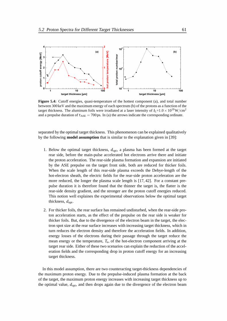
5.2 Proton Spectra for Different Target Thicknesses 61
Figure 5.4: Cutoff energies, quasi-temperature of the hottest component (a), and total numberbetween 300keV and the maximum energy of each spectrum (b) ofthe protons as a function of thetarget thickness. The aluminum foils were irradiated at a laser intensity ofIL=1.0×10¹⁹W/cm2
and a prepulse duration ofτASE = 700ps. In (a) the arrows indicate the corresponding ordinate.
separated by the optimal target thickness. This phenomenoncan be explained qualitativelyby the followingmodel assumptionthat is similar to the explanation given in [39]:
1. Below the optimal target thickness,dopt, a plasma has been formed at the targetrear side, before the main-pulse accelerated hot electronsarrive there and initiatethe proton acceleration. The rear-side plasma formation and expansion are initiatedby the ASE prepulse on the target front side, both are reducedfor thicker foils.When the scale length of this rear-side plasma exceeds the Debye-length of thehot-electron sheath, the electric fields for the rear-side proton acceleration are themore reduced, the longer the plasma scale length is [17, 42].For a constant pre-pulse duration it is therefore found that the thinner the target is, the flatter is therear-side density gradient, and the stronger are the protoncutoff energies reduced.This notion well explaines the experimental observations below the optimal targetthickness,dopt.
2. For thicker foils, the rear surface has remained undisturbed, when the rear-side pro-ton acceleration starts, as the effect of the prepulse on therear side is weaker forthicker foils. But, due to the divergence of the electron beam in the target, the elec-tron spot size at the rear surface increases with increasingtarget thickness, which inturn reduces the electron density and therefore the acceleration fields. In addition,energy losses of the electrons during their passage throughthe target reduce themean energy or the temperature,Te, of the hot-electron component arriving at thetarget rear side. Either of these two scenarios can explain the reduction of the accel-eration fields and the corresponding drop in proton cutoff energy for an increasingtarget thickness.
In this model assumption, there are two counteracting target-thickness dependencies ofthe maximum proton energy. Due to the prepulse-induced plasma formation at the backof the target, the maximum proton energy increases with increasing target thickness up tothe optimal value,dopt, and then drops again due to the divergence of the electron beam
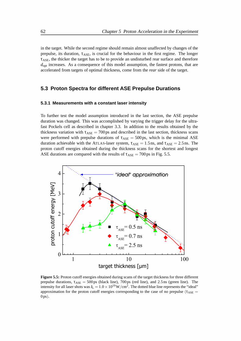
62 Chapter 5 Proton Acceleration in the Experiment
in the target. While the second regime should remain almost unaffected by changes of theprepulse, its duration,τASE, is crucial for the behaviour in the first regime. The longerτASE, the thicker the target has to be to provide an undisturbed rear surface and thereforedopt increases. As a consequence of this model assumption, the fastest protons, that areaccelerated from targets of optimal thickness, come from the rear side of the target.
5.3 Proton Spectra for different ASE Prepulse Durations
5.3.1 Measurements with a constant laser intensity
To further test the model assumption introduced in the last section, the ASE prepulseduration was changed. This was accomplished by varying the trigger delay for the ultra-fast Pockels cell as described in chapter 3.3. In addition tothe results obtained by thethickness variation withτASE = 700ps and described in the last section, thickness scanswere performed with prepulse durations ofτASE = 500ps, which is the minimal ASEduration achievable with the ATLAS-laser system,τASE = 1.5ns, andτASE = 2.5ns. Theproton cutoff energies obtained during the thickness scansfor the shortest and longestASE durations are compared with the results ofτASE = 700ps in Fig. 5.5.
Figure 5.5: Proton cutoff energies obtained during scans of the target thickness for three differentprepulse durations,τASE = 500ps (black line), 700ps (red line), and 2.5ns (green line). Theintensity for all laser shots wasIL = 1.0×10¹⁹W/cm2. The dotted blue line represents the “ideal”approximation for the proton cutoff energies corresponding to the case of no prepulse(τASE =0ps).
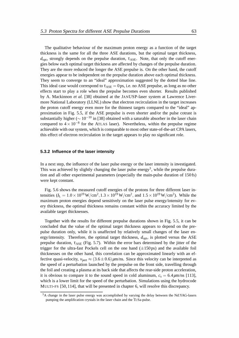
5.3 Proton Spectra for different ASE Prepulse Durations 63
The qualitative behaviour of the maximum proton energy as a function of the targetthickness is the same for all the three ASE durations, but theoptimal target thickness,dopt, strongly depends on the prepulse duration,τASE. Note, that only the cutoff ener-gies below each optimal target thickness are affected by changes of the prepulse duration.They are the more reduced the longer the ASE prepulse is. On the other hand, the cutoffenergies appear to be independent on the prepulse duration above each optimal thickness.They seem to converge to an “ideal” approximation suggestedby the dotted blue line.This ideal case would correspond toτASE = 0ps, i.e. no ASE prepulse, as long as no othereffects start to play a role when the prepulse becomes even shorter. Results publishedby A. Mackinnonet al. [38] obtained at the JANUSP-laser system at Lawrence Liver-more National Laboratory (LLNL) show that electron recirculation in the target increasesthe proton cutoff energy even more for the thinnest targets compared to the “ideal” ap-proximation in Fig. 5.5, if the ASE prepulse is even shorter and/or the pulse cotrast issubstantially higher (∼ 10−10 in [38] obtained with a saturable absorber in the laser chaincompared to 4×10⁻⁸ for the ATLAS laser). Nevertheless, within the prepulse regimeachievable with our system, which is comparable to most other state-of-the-art CPA lasers,this effect of electron recirculation in the target appearsto play no significant role.
5.3.2 Influence of the laser intensity
In a next step, the influence of the laser pulse energy or the laser intensity is investigated.This was achieved by slightly changing the laser pulse energy3, while the prepulse dura-tion and all other experimental parameters (especially themain-pulse duration of 150fs)were kept constant.
Fig. 5.6 shows the measured cutoff energies of the protons for three different laser in-tensities (IL = 1.0×10¹⁹W/cm2,1.3×1019W/cm2, and 1.5×10¹⁹W/cm2). While themaximum proton energies depend sensitively on the laser pulse energy/intensity for ev-ery thickness, the optimal thickness remains constant within the accuracy limited by theavailable target thicknesses.
Together with the results for different prepulse durationsshown in Fig. 5.5, it can beconcluded that the value of the optimal target thickness appears to depend on the pre-pulse duration only, while it is unaffected by relatively small changes of the laser en-ergy/intensity. Therefore, the optimal target thickness,dopt, is plotted versus the ASEprepulse duration,τASE (Fig. 5.7). Within the error bars determined by the jitter ofthetrigger for the ultra-fast Pockels cell on the one hand (±150ps) and the available foilthicknesses on the other hand, this correlation can be approximated linearly with an ef-fective quasi-velocity,vpert≈ (3.6±0.6)µm/ns. Since this velocity can be interpreted asthe speed of a perturbation launched by the prepulse on the front side, travelling throughthe foil and creating a plasma at its back side that affects the rear-side proton acceleration,it is obvious to compare it to the sound speed in cold aluminum, cs = 6.4µm/ns [113],which is a lower limit for the speed of the perturbation. Simulations using the hydrocodeMULTI -FS [50,114], that will be presented in chapter 6, will resolve this discrepancy.
3A change in the laser pulse energy was accomplished by varying the delay between the Nd:YAG-laserspumping the amplification crystals in the laser chain and theTi:Sa-pulse.

64 Chapter 5 Proton Acceleration in the Experiment
Figure 5.6: Proton cutoff energies for three different laser intensities achieved by changing themain-pulse energy. While the prepulse duration for all the laser shots was kept constant atτASE =2.5ns, the laser intensity was varied betweenIL = 1.0×10¹⁹W/cm2 andIL = 1.5×10¹⁹W/cm2.Although the cutoff energies strongly depend on the laser intensity, the optimal target thicknessremains unaffected.
5.3.3 Correlated Changes in the Spatial Profiles of the Proto n Beam
To describe two further aspects concerning the energy spectra and the beam profiles ofthe protons, that also change when approaching the optimal target thickness, the re-sults obtained with a prepulse duration ofτASE = 2.5ns and a laser intensity ofIL =1.3×10¹⁹W/cm2 are investigated in more detail. In section 5.2, target-thickness depen-dencies both for the cutoff energy and the temperature of thehot proton component werealready found (cf. Fig. 5.4).
For the longer prepulse duration ofτASE = 2.5ns, this behaviour is even more pro-nounced, as a longer prepulse is capable of producing a rear-side plasma with a longerdensity-scale length. The proton spectra for three foil thicknesses approaching the opti-mal target thickness (dopt = 8.5µm for this prepulse duration) are shown in Fig. 5.8 (a)together with the spatial beam profiles (b)−(d), that were recorded simultaneously. Theinset of Fig. 5.8 (a) compares the cutoff energies with the temperature of the hottest protoncomponent for all foils used with thicknesses between 1.5 and 30µm.
Starting at the foil thickness of 5µm, a second hotter component appears in the pro-ton spectra having its highest quasi-temperature of(4.0±0.6)MeV at the optimal targetthickness. At and above this thickness, a clear two-temperature distribution is obtainedin the energy spectrum. The cutoff energies match the temperature of the hot component
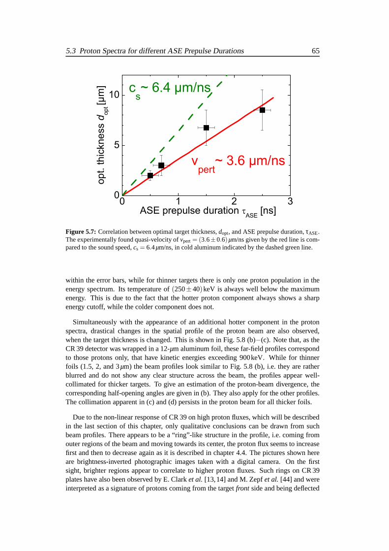
5.3 Proton Spectra for different ASE Prepulse Durations 65
Figure 5.7: Correlation between optimal target thickness,dopt, and ASE prepulse duration,τASE.The experimentally found quasi-velocity ofvpert = (3.6±0.6)µm/ns given by the red line is com-pared to the sound speed,cs = 6.4µm/ns, in cold aluminum indicated by the dashed green line.
within the error bars, while for thinner targets there is only one proton population in theenergy spectrum. Its temperature of(250±40)keV is always well below the maximumenergy. This is due to the fact that the hotter proton component always shows a sharpenergy cutoff, while the colder component does not.
Simultaneously with the appearance of an additional hottercomponent in the protonspectra, drastical changes in the spatial profile of the proton beam are also observed,when the target thickness is changed. This is shown in Fig. 5.8 (b)−(c). Note that, as theCR 39 detector was wrapped in a 12-µm aluminum foil, these far-field profiles correspondto those protons only, that have kinetic energies exceeding900keV. While for thinnerfoils (1.5, 2, and 3µm) the beam profiles look similar to Fig. 5.8 (b), i.e. they areratherblurred and do not show any clear structure across the beam, the profiles appear well-collimated for thicker targets. To give an estimation of theproton-beam divergence, thecorresponding half-opening angles are given in (b). They also apply for the other profiles.The collimation apparent in (c) and (d) persists in the proton beam for all thicker foils.
Due to the non-linear response of CR 39 on high proton fluxes, which will be describedin the last section of this chapter, only qualitative conclusions can be drawn from suchbeam profiles. There appears to be a “ring”-like structure inthe profile, i.e. coming fromouter regions of the beam and moving towards its center, the proton flux seems to increasefirst and then to decrease again as it is described in chapter 4.4. The pictures shown hereare brightness-inverted photographic images taken with a digital camera. On the firstsight, brighter regions appear to correlate to higher proton fluxes. Such rings on CR 39plates have also been observed by E. Clarket al. [13,14] and M. Zepfet al. [44] and wereinterpreted as a signature of protons coming from the targetfront side and being deflected
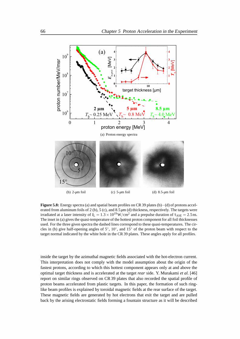
66 Chapter 5 Proton Acceleration in the Experiment
(a) Proton energy spectra
15°
10°
5°
(b) 2-µm foil (c) 5-µm foil (d) 8.5-µm foil
Figure 5.8: Energy spectra (a) and spatial beam profiles on CR 39 plates (b)−(d) of protons accel-erated from aluminum foils of 2 (b), 5 (c), and 8.5µm (d) thickness, respectively. The targets wereirradiated at a laser intensity ofIL = 1.3×10¹⁹W/cm2 and a prepulse duration ofτASE = 2.5ns.The inset in (a) gives the quasi-temperature of the hottest proton component for all foil thicknessesused. For the three given spectra the dashed lines correspond to these quasi-temperatures. The cir-cles in (b) give half-opening angles of 5, 10, and 15 of the proton beam with respect to thetarget normal indicated by the white hole in the CR 39 plates.These angles apply for all profiles.
inside the target by the azimuthal magnetic fields associated with the hot-electron current.This interpretation does not comply with the model assumption about the origin of thefastest protons, according to which this hottest componentappears only at and above theoptimal target thickness and is accelerated at the targetrear side. Y. Murakamiet al. [46]report on similar rings observed on CR 39 plates that also recorded the spatial profile ofproton beams accelerated from plastic targets. In this paper, the formation of such ring-like beam profiles is explained by toroidal magnetic fields atthe rear surface of the target.These magnetic fields are generated by hot electrons that exit the target and are pulledback by the arising electrostatic fields forming a fountain structure as it will be described
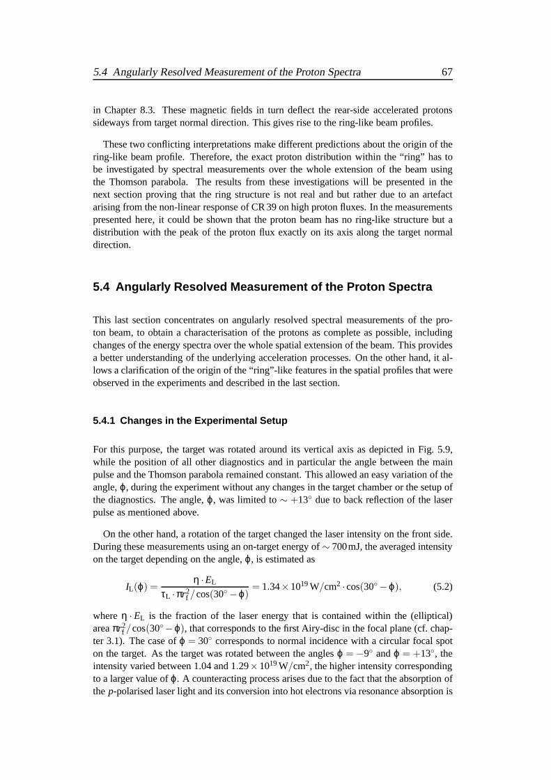
5.4 Angularly Resolved Measurement of the Proton Spectra 67
in Chapter 8.3. These magnetic fields in turn deflect the rear-side accelerated protonssideways from target normal direction. This gives rise to the ring-like beam profiles.
These two conflicting interpretations make different predictions about the origin of thering-like beam profile. Therefore, the exact proton distribution within the “ring” has tobe investigated by spectral measurements over the whole extension of the beam usingthe Thomson parabola. The results from these investigations will be presented in thenext section proving that the ring structure is not real and but rather due to an artefactarising from the non-linear response of CR 39 on high proton fluxes. In the measurementspresented here, it could be shown that the proton beam has no ring-like structure but adistribution with the peak of the proton flux exactly on its axis along the target normaldirection.
5.4 Angularly Resolved Measurement of the Proton Spectra
This last section concentrates on angularly resolved spectral measurements of the pro-ton beam, to obtain a characterisation of the protons as complete as possible, includingchanges of the energy spectra over the whole spatial extension of the beam. This providesa better understanding of the underlying acceleration processes. On the other hand, it al-lows a clarification of the origin of the “ring”-like features in the spatial profiles that wereobserved in the experiments and described in the last section.
5.4.1 Changes in the Experimental Setup
For this purpose, the target was rotated around its verticalaxis as depicted in Fig. 5.9,while the position of all other diagnostics and in particular the angle between the mainpulse and the Thomson parabola remained constant. This allowed an easy variation of theangle,ϕ, during the experiment without any changes in the target chamber or the setup ofthe diagnostics. The angle,ϕ, was limited to∼ +13 due to back reflection of the laserpulse as mentioned above.
On the other hand, a rotation of the target changed the laser intensity on the front side.During these measurements using an on-target energy of∼ 700mJ, the averaged intensityon the target depending on the angle,ϕ, is estimated as
IL(ϕ) =η ·EL
τL ·πr2f /cos(30−ϕ)
= 1.34×10¹⁹W/cm2 ·cos(30−ϕ), (5.2)
whereη ·EL is the fraction of the laser energy that is contained within the (elliptical)areaπr2
f /cos(30−ϕ), that corresponds to the first Airy-disc in the focal plane (cf. chap-ter 3.1). The case ofϕ = 30 corresponds to normal incidence with a circular focal spoton the target. As the target was rotated between the anglesϕ = −9 andϕ = +13, theintensity varied between 1.04 and 1.29×10¹⁹W/cm2, the higher intensity correspondingto a larger value ofϕ. A counteracting process arises due to the fact that the absorption ofthep-polarised laser light and its conversion into hot electrons via resonance absorption is

68 Chapter 5 Proton Acceleration in the Experiment
Figure 5.9: Experimen-tal setup for the angularly re-solved measurements of theproton spectra. While the an-gle between main pulse andThomson parabola remainsfixed, the target is rotatedaround its vertical axis by theangle, ϕ. The rotated tar-get corresponds toϕ = +13.As the proton beam is emittedalong the target normal direc-tion, its imprint on the CR 39plates is shifted correspond-ingly. The Thomson parabolathen measures the spectrumunder an angle,ϕ, from targetnormal direction.
target
to Thomsonparabola
ATLAS 10-beam
( -polarised)p
CR 39
j
j
enhanced for larger incident angles [59]. To some extent, this increased absorption mightbalance the associated reduction of the laser intensity. Furthermore, as the preplasma evo-lution on the target front side is a mixture of both a plane anda radial expansion, resultingin a convex sphere of the critical density where the laser light is absorbed, any effectsassociated with a rotation of the target are additionally reduced.
5.4.2 Measurement of Proton-Energy Spectra and Beam Profile s
Fig. 5.10 shows both the energy spectra (a) and the beam profiles (b)−(e) of the protonsobtained for four different anglesϕ (−7,0,+5, and+13). It is obvious that the beamprofiles move as to follow the target rotation. The center of the profile is always rotatedby the same angle as the target with an accuracy of±1, which was also the accuracy ofthe target alignment. This is in full agreement with the factthat similar proton featuresobserved in different experiments [15,28] always appearedin the direction of the rear-sidetarget normal.
The energy spectra of the protons were measured simultaneously in a direction corre-sponding to the position in the spatial profile that is indicated by the hole in the CR 39plate. These holes are either in the center of the beam (c) where the proton flux appearsto be lower or in the outer regions (b), (d), and (e) with apparently higher fluxes. Butwhen comparing the beam profiles with the exact energy spectra (a), it can be concludedunambigously that in the center of the beam, i.e. forϕ = 0, the highest proton numbersare obtained and the larger the deviation from the center is,the more is the total protonnumber reduced. This clearly rules out a ring-like beam profile as in [13, 14, 46]. A de-tailed investigation of the CR 39 plates under an optical microscope reveals that comingfrom outer regions (i.e. from large anglesϕ), the proton pits are well separated in thebeginning but then start to overlap corresponding to a region on the CR 39 which appears
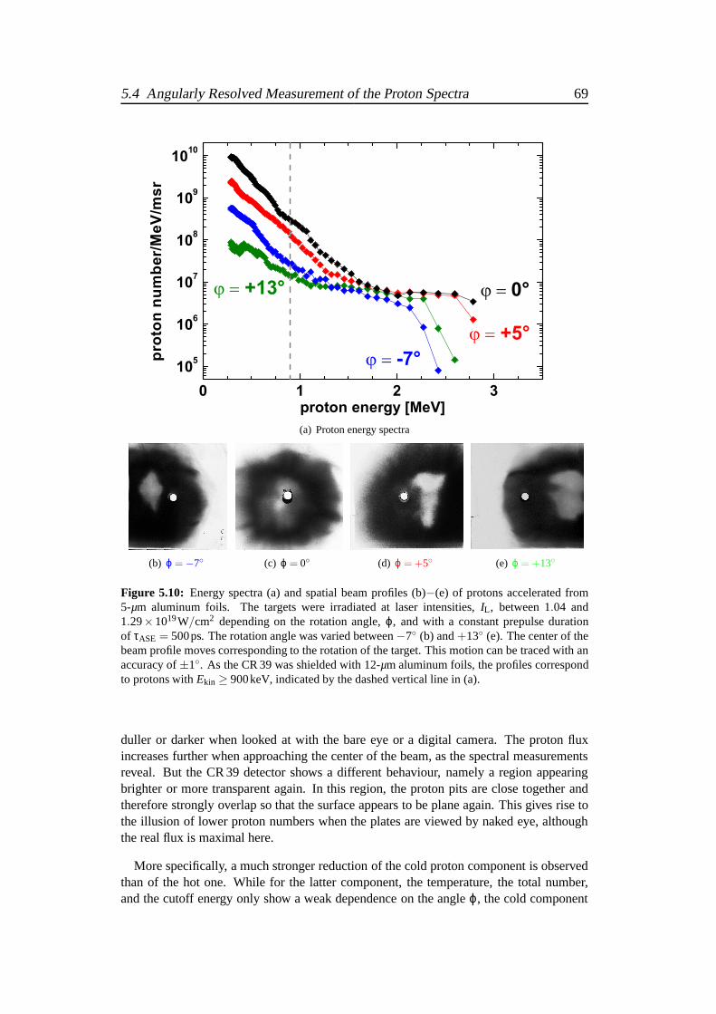
5.4 Angularly Resolved Measurement of the Proton Spectra 69
(a) Proton energy spectra
(b) ϕ = −7 (c) ϕ = 0 (d) ϕ = +5 (e) ϕ = +13
Figure 5.10: Energy spectra (a) and spatial beam profiles (b)−(e) of protons accelerated from5-µm aluminum foils. The targets were irradiated at laser intensities, IL , between 1.04 and1.29×1019W/cm2 depending on the rotation angle,ϕ, and with a constant prepulse durationof τASE = 500ps. The rotation angle was varied between−7 (b) and+13 (e). The center of thebeam profile moves corresponding to the rotation of the target. This motion can be traced with anaccuracy of±1. As the CR 39 was shielded with 12-µm aluminum foils, the profiles correspondto protons withEkin ≥ 900keV, indicated by the dashed vertical line in (a).
duller or darker when looked at with the bare eye or a digital camera. The proton fluxincreases further when approaching the center of the beam, as the spectral measurementsreveal. But the CR 39 detector shows a different behaviour, namely a region appearingbrighter or more transparent again. In this region, the proton pits are close together andtherefore strongly overlap so that the surface appears to beplane again. This gives rise tothe illusion of lower proton numbers when the plates are viewed by naked eye, althoughthe real flux is maximal here.
More specifically, a much stronger reduction of the cold proton component is observedthan of the hot one. While for the latter component, the temperature, the total number,and the cutoff energy only show a weak dependence on the angleϕ, the cold component
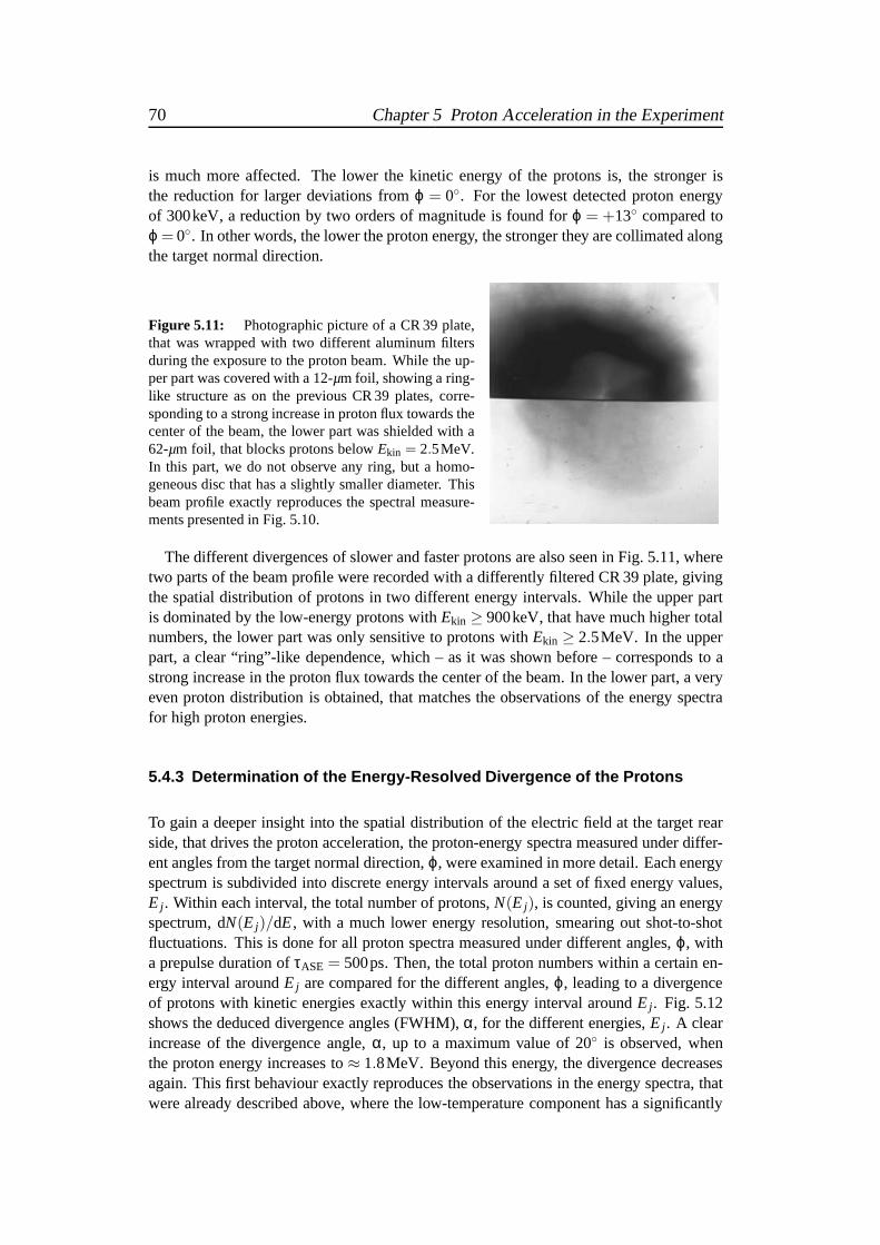
70 Chapter 5 Proton Acceleration in the Experiment
is much more affected. The lower the kinetic energy of the protons is, the stronger isthe reduction for larger deviations fromϕ = 0. For the lowest detected proton energyof 300keV, a reduction by two orders of magnitude is found forϕ = +13 compared toϕ = 0. In other words, the lower the proton energy, the stronger they are collimated alongthe target normal direction.
Figure 5.11: Photographic picture of a CR 39 plate,that was wrapped with two different aluminum filtersduring the exposure to the proton beam. While the up-per part was covered with a 12-µm foil, showing a ring-like structure as on the previous CR 39 plates, corre-sponding to a strong increase in proton flux towards thecenter of the beam, the lower part was shielded with a62-µm foil, that blocks protons belowEkin = 2.5MeV.In this part, we do not observe any ring, but a homo-geneous disc that has a slightly smaller diameter. Thisbeam profile exactly reproduces the spectral measure-ments presented in Fig. 5.10.
The different divergences of slower and faster protons are also seen in Fig. 5.11, wheretwo parts of the beam profile were recorded with a differentlyfiltered CR 39 plate, givingthe spatial distribution of protons in two different energyintervals. While the upper partis dominated by the low-energy protons withEkin ≥ 900keV, that have much higher totalnumbers, the lower part was only sensitive to protons withEkin ≥ 2.5MeV. In the upperpart, a clear “ring”-like dependence, which – as it was shownbefore – corresponds to astrong increase in the proton flux towards the center of the beam. In the lower part, a veryeven proton distribution is obtained, that matches the observations of the energy spectrafor high proton energies.
5.4.3 Determination of the Energy-Resolved Divergence of t he Protons
To gain a deeper insight into the spatial distribution of theelectric field at the target rearside, that drives the proton acceleration, the proton-energy spectra measured under differ-ent angles from the target normal direction,ϕ, were examined in more detail. Each energyspectrum is subdivided into discrete energy intervals around a set of fixed energy values,E j . Within each interval, the total number of protons,N(E j), is counted, giving an energyspectrum, dN(E j)/dE, with a much lower energy resolution, smearing out shot-to-shotfluctuations. This is done for all proton spectra measured under different angles,ϕ, witha prepulse duration ofτASE = 500ps. Then, the total proton numbers within a certain en-ergy interval aroundE j are compared for the different angles,ϕ, leading to a divergenceof protons with kinetic energies exactly within this energyinterval aroundE j . Fig. 5.12shows the deduced divergence angles (FWHM),α, for the different energies,E j . A clearincrease of the divergence angle,α, up to a maximum value of 20 is observed, whenthe proton energy increases to≈ 1.8MeV. Beyond this energy, the divergence decreasesagain. This first behaviour exactly reproduces the observations in the energy spectra, thatwere already described above, where the low-temperature component has a significantly
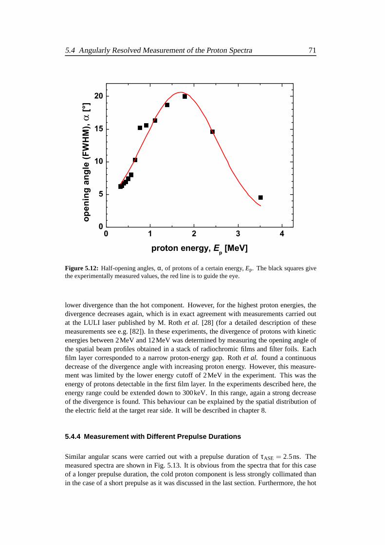
5.4 Angularly Resolved Measurement of the Proton Spectra 71
Figure 5.12: Half-opening angles,α, of protons of a certain energy,Ep. The black squares givethe experimentally measured values, the red line is to guidethe eye.
lower divergence than the hot component. However, for the highest proton energies, thedivergence decreases again, which is in exact agreement with measurements carried outat the LULI laser published by M. Rothet al. [28] (for a detailed description of thesemeasurements see e.g. [82]). In these experiments, the divergence of protons with kineticenergies between 2MeV and 12MeV was determined by measuringthe opening angle ofthe spatial beam profiles obtained in a stack of radiochromicfilms and filter foils. Eachfilm layer corresponded to a narrow proton-energy gap. Rothet al. found a continuousdecrease of the divergence angle with increasing proton energy. However, this measure-ment was limited by the lower energy cutoff of 2MeV in the experiment. This was theenergy of protons detectable in the first film layer. In the experiments described here, theenergy range could be extended down to 300keV. In this range,again a strong decreaseof the divergence is found. This behaviour can be explained by the spatial distribution ofthe electric field at the target rear side. It will be described in chapter 8.
5.4.4 Measurement with Different Prepulse Durations
Similar angular scans were carried out with a prepulse duration of τASE = 2.5ns. Themeasured spectra are shown in Fig. 5.13. It is obvious from the spectra that for this caseof a longer prepulse duration, the cold proton component is less strongly collimated thanin the case of a short prepulse as it was discussed in the last section. Furthermore, the hot
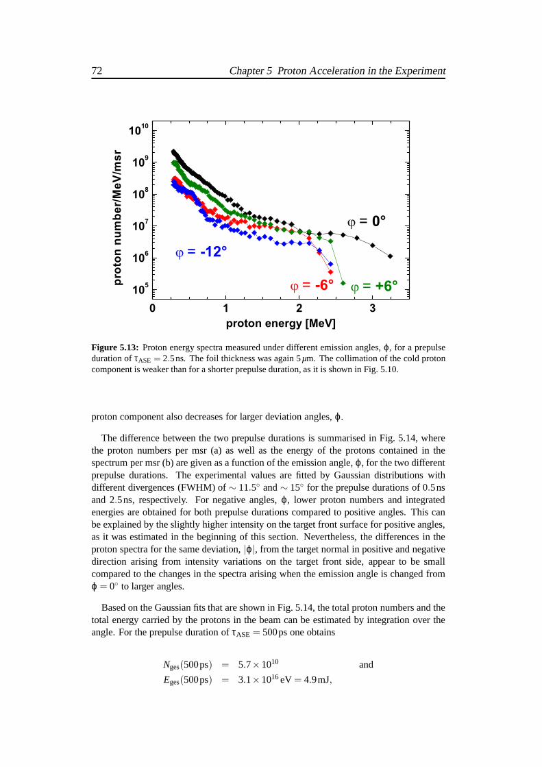
72 Chapter 5 Proton Acceleration in the Experiment
Figure 5.13: Proton energy spectra measured under different emission angles,ϕ, for a prepulseduration ofτASE = 2.5ns. The foil thickness was again 5µm. The collimation of the cold protoncomponent is weaker than for a shorter prepulse duration, asit is shown in Fig. 5.10.
proton component also decreases for larger deviation angles, ϕ.
The difference between the two prepulse durations is summarised in Fig. 5.14, wherethe proton numbers per msr (a) as well as the energy of the protons contained in thespectrum per msr (b) are given as a function of the emission angle,ϕ, for the two differentprepulse durations. The experimental values are fitted by Gaussian distributions withdifferent divergences (FWHM) of∼ 11.5 and∼ 15 for the prepulse durations of 0.5nsand 2.5ns, respectively. For negative angles,ϕ, lower proton numbers and integratedenergies are obtained for both prepulse durations comparedto positive angles. This canbe explained by the slightly higher intensity on the target front surface for positive angles,as it was estimated in the beginning of this section. Nevertheless, the differences in theproton spectra for the same deviation,|ϕ|, from the target normal in positive and negativedirection arising from intensity variations on the target front side, appear to be smallcompared to the changes in the spectra arising when the emission angle is changed fromϕ = 0 to larger angles.
Based on the Gaussian fits that are shown in Fig. 5.14, the total proton numbers and thetotal energy carried by the protons in the beam can be estimated by integration over theangle. For the prepulse duration ofτASE = 500ps one obtains
Nges(500ps) = 5.7×10¹⁰ and
Eges(500ps) = 3.1×10¹⁶eV = 4.9mJ,

5.4 Angularly Resolved Measurement of the Proton Spectra 73
(a) Proton number per solid angle
(b) Energy carried by the protons per solid angle
Figure 5.14: Proton number per solid angle (a) and energy carried by the protons per msr (b) asa function of the emission angle,ϕ, for two prepulse durations of 500ps (black diamonds) and2.5ns (red diamonds). The dashed lines are Gaussian fits to the experimental data, yielding inboth plots divergences (FWHM) of 11.5 and 15 for the prepulse durations of 500ps and 2.5ns,respectively.
while for the longer prepulse ofτASE = 2.5ns
Nges(2.5ns) = 3.0×10¹⁰ and
Eges(2.5ns) = 1.5×10¹⁶eV = 2.4mJ
is found. The conversion efficiency of laser-pulse energy (EL ≈ 700mJ for these shots)into protons with kinetic energies exceeding 300keV is therefore 0.7% and 0.34% for theprepulse durations of 500ps and 2.5ns, respectively.
74 Chapter 5 Proton Acceleration in the Experiment
5.5 Summary of the Experimental Observations
The experimental findings concerning the characterisationof the laser-accelerated protonbeam can be summarised as follows:
• A strong dependence of the appearance of one or more temperatures in the energyspectra, the total number, and the maximum kinetic energy ofthe protons on thealuminum-foil thickness was demonstrated. An optimal target thickness,dopt, wasfound at which the proton cutoff energy and the temperature of the hottest compo-nent in the spectrum are maximal.
• By a controlled variation of the ASE prepulse duration,τASE, a clear correlationbetween the optimal target thickness and the prepulse duration was found. Thiscorrelation is approximately linear.
• While the proton cutoff energy strongly depends on the laser-pulse energy and thecombination of target thickness and prepulse duration, theoptimal target thickness,dopt, depends on the prepulse duration only.
• The proton spectra and the spatial beam profiles change significantly arounddopt, acorrelated appearance both of a significantly hotter protoncomponent in the energyspectrum and of a collimated feature in the beam profiles, exactly aligned along thetarget normal direction was observed.
• The “ring”-like structure in the beam profiles recorded on CR39 plates is not realbut an artefact of the non-linear response of the detector onhigh proton fluxes. Thiswas proven by angularly resolved measurements of the protonspectra revealing astrong collimation of the cold proton component and a large divergence of the hottercomponent for short prepulses.
• The proton divergence strongly depends on their kinetic energy. While for energiesabove 2MeV the divergence decreases with the proton energy,what is in exactagreement with measurements from other groups, a strong collimation of the lowenergy protons could be demonstrated for the first time.
• The total number of protons accelerated from a 5-µm aluminum foil to energiesabove 300keV is 5.7×10¹⁰ and 3.0×10¹⁰ for the prepulse durations of 500ps and2.5ns, respectively. These protons carry a total energy of 4.9mJ (τASE = 500ps) and2.4mJ (τASE = 2.5ns) yielding a conversion efficiency of 0.7% and 0.34% from alaser-pulse energy ofEL ≈ 700mJ into protons.

Chapter 6
Influence of the Laser Prepulse:Simulations with the Code MULTI-FS
In the experiments described in chapter 5, a strong influenceof the laser prepulse duration,τASE, on the acceleration of protons was observed. The highest kinetic proton energieswere achieved with foils having an optimal thickness,dopt. This optimal thickness wasfound to increase with increasing prepulse duration (cf. Figs. 5.5 and 5.7). This behaviourcould be explained qualitatively by assuming that prepulse-induced changes in the targetproperties such as an expansion of the target and a formationof a rear-side ion-densitygradient strongly influence the rear-side acceleration. Triggered by the prepulse imping-ing on the front side, it appears natural that the changes at the rear side of the target dependon its thickness. This chapter deals with the quantitative description of prepulse-inducedeffects on the target properties by means of numerical simulations.
6.1 Motivation for Hydro Simulations
The effect of the ASE prepulse on the rear-side accelerationof protons was observed forthe first time by M. Rothet al. in experiments using gold targets, that were irradiated withslightly higher laser intensities [37]. In these experiments, the number of protons withkinetic energies above the detection threshold of∼ 2MeV were compared for two differ-ent prepulse durations using targets with a constant thickness of 48µm. For a prepulse of5ns duration having an intensity level of∼ 5×10¹²W/cm2, a strong proton signal wasobserved, while for a 10-ns prepulse, no protons with energies exceeding 2MeV couldbe detected. These two experimental values only allow a rough estimate of the influenceof the prepulse. Based on results from MULTI simulations [114], the authors concludedthat the break-out of a shock wave at the back of the target that has been launched bythe prepulse on the front side and has travelled through the target was responsible for thediminution of the proton cutoff energy below the detection threshold of 2MeV.
For the experiments presented in this thesis with slightly different laser conditions,especially a much lower prepulse intensity level, which could be carried out in muchgreater detail and with higher accuracy, the shock wave propagating through the materialalone is not sufficient to explain the results. To gain a deeper insight into the processesinvolved, detailed simulations using the code MULTI -FS [50] were carried out. Thesesimulations give a plausible explanation for the experimental results.
75

76 Chapter 6 Simulations withMULTI -FS
6.2 The 1-D Hydrodynamic Code MULTI-FS
The one-dimensional hydrodynamic code MULTI -FS [50] is an extended version of thecode MULTI [114] developed to describe the radiation hydrodynamics inexperimentsrelevant for inertial confinement fusion. Both versions of the code describe the hydrody-namic processes in solid targets triggered by laser irradiation. The code uses Lagrangiancoordinates [115] including electronic heat conduction and multigroup radiation transport.In Lagrangian coordinates the density, pressure, and velocity of the target material are notdetermined at afixed position in spaceas in Eulerian coordinates, but the changes of thesequantities are described for afluid elementthat moves in space. Initially, the target foilis subdivided into thin layers, each representing such a 1-Dfluid element. The temporalevolution of each layer is described by the basic equations of hydrodynamics [115] thatexpress the conservation of mass, momentum, and total energy in each layer. The internalenergy of each fluid element can be changed by changing its volume, by electronic heatconduction, and by the absorption and emission of radiation. The hydrodynamic equa-tions have to be completed by equations of state (EOS) for theinternal energy and thepressure as functions of the local density and temperature.This is implemented into thecode by tabulated values obtained from the Los Alamos SESAME EOS [116]. The codetreats radiative effects by using tabulated values for the (frequency-dependent) radiativeabsorption and emission coefficients that are also functions of density and temperature.These tabulated values (also called opacity tables) are obtained from the SNOP atomicphysics code, as it is described in [117].
While in MULTI , the laser-light absorption is described by Beer’s law thatonly holdstrue for shallow plasma gradients (density-scale lengthLp λL), MULTI -FS explic-itly solves Maxwell’s equations to correctly describe the light absorption also in steep-gradient plasmas. Furthermore, MULTI -FS includes a more realistic model for the electri-cal and thermal conductivity in the target covering a wide range of densities and tempera-tures. As the intensity of the ASE prepulse as well as the initial temperature of the targetmaterial were very low in the experiments described in this thesis, a correct descriptionof the cold solid state in the simulation is of great importance. The energy exchange be-tween electrons and ions as well as the thermal conductivityof the material depend on theelectron-collision frequency,νe. In a plasma at high temperatures, the electron collisionsare Coulomb-like, andνe is described by Spitzer’s law. Here,νe is proportional toTe
−3/2,but for low electron temperatures, the collision frequencywould diverge in this model.However, in a solid below the Fermi temperature,TF, which is 11.7eV for aluminum, theelectrons are in a degenerate state, and the collision frequency no longer depends on theelectron temperature, but it is governed by the scattering of electrons by lattice vibrations(phonons). In this case,νe is proportional to the temperature of the ions,Ti. Here,νe
converges for low temperatures. In MULTI -FS, a formula interpolated between these tworegimes is utilized to correctly describe the thermal conductivity in aluminum in all statesranging from the solid state at room temperature up to the plasma state. Furthermore,MULTI -FS uses separate SESAME EOS for electrons and ions, what becomes the moreimportant, the lower the initial temperatures are. This allows realistic simulations withintensities and initial temperatures as low as in the experiments reported here.

6.3 Details of the Simulations 77
6.3 Details of the Simulations
The simulation starts with an aluminum target that is initially at room temperature (kBTe =kBTi = 0.03eV). The laser pulse implemented into the code follows themeasured ASE-prepulse evolution that is again shown in Fig. 6.1. For the different prepulse durations,
Figure 6.1: Linear fits (dashed lines) to the measured (solid lines) temporal evolution of the ASEintensity for different prepulse durations. The three solid lines correspond toτASE = 2.5ns (blue),1.0ns (red), and 0.5ns (black), respectively. Att = 0 the main pulse starts, what is no longerincluded in the MULTI -FSsimulations. Duringτrise, the prepulse-intensity increases linearly to itsmaximum value of 8×10¹¹W/cm2.
τASE, used in the experiment, the ASE prepulse is modeled in the following way. Its inten-sity rises linearly from 0 to 8×10¹¹W/cm2 within a certain rise time,τrise, that slightlychanges for the different prepulse durations. The peak ASE intensity corresponds to arelative ASE level of 4×10⁻⁸ for a main pulse intensity ofIL = 2×10¹⁹W/cm2, whichwas the peak intensity on the target in our experiments assuming the same focusability ofprepulse and main pulse. After the time equivalent to the prepulse duration, the simulationgives the target properties at the moment of the main pulse arrival.
Fig. 6.2 shows the schematic initial cell layout used in the simulations. The laser im-pinges onto the target from the left. The cell widths in the front- (A) and rear-side part(C) of the target decrease towards the surfaces to describe thelaser-target interaction atthe front and the rear-side plasma evolution at the back of the target with higher accuracy.The central part (B) has a constant cell width, the cell number is varied to obtain differenttotal target thicknesses.
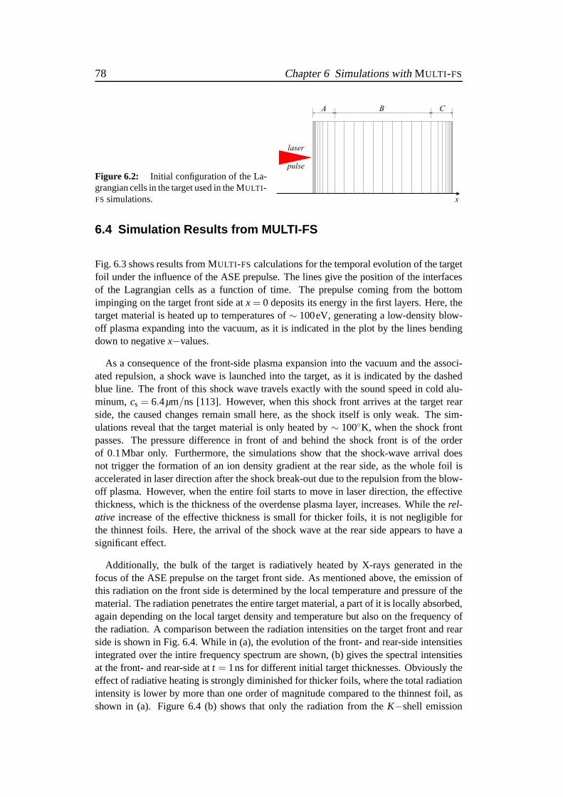
78 Chapter 6 Simulations withMULTI -FS
Figure 6.2: Initial configuration of the La-grangian cells in the target used in the MULTI -FS simulations.
BA C
x
laser
pulse
6.4 Simulation Results from MULTI-FS
Fig. 6.3 shows results from MULTI -FS calculations for the temporal evolution of the targetfoil under the influence of the ASE prepulse. The lines give the position of the interfacesof the Lagrangian cells as a function of time. The prepulse coming from the bottomimpinging on the target front side atx = 0 deposits its energy in the first layers. Here, thetarget material is heated up to temperatures of∼ 100eV, generating a low-density blow-off plasma expanding into the vacuum, as it is indicated in the plot by the lines bendingdown to negativex−values.
As a consequence of the front-side plasma expansion into thevacuum and the associ-ated repulsion, a shock wave is launched into the target, as it is indicated by the dashedblue line. The front of this shock wave travels exactly with the sound speed in cold alu-minum,cs = 6.4µm/ns [113]. However, when this shock front arrives at the target rearside, the caused changes remain small here, as the shock itself is only weak. The sim-ulations reveal that the target material is only heated by∼ 100K, when the shock frontpasses. The pressure difference in front of and behind the shock front is of the orderof 0.1Mbar only. Furthermore, the simulations show that the shock-wave arrival doesnot trigger the formation of an ion density gradient at the rear side, as the whole foil isaccelerated in laser direction after the shock break-out due to the repulsion from the blow-off plasma. However, when the entire foil starts to move in laser direction, the effectivethickness, which is the thickness of the overdense plasma layer, increases. While therel-ative increase of the effective thickness is small for thicker foils, it is not negligible forthe thinnest foils. Here, the arrival of the shock wave at therear side appears to have asignificant effect.
Additionally, the bulk of the target is radiatively heated by X-rays generated in thefocus of the ASE prepulse on the target front side. As mentioned above, the emission ofthis radiation on the front side is determined by the local temperature and pressure of thematerial. The radiation penetrates the entire target material, a part of it is locally absorbed,again depending on the local target density and temperaturebut also on the frequency ofthe radiation. A comparison between the radiation intensities on the target front and rearside is shown in Fig. 6.4. While in (a), the evolution of the front- and rear-side intensitiesintegrated over the intire frequency spectrum are shown, (b) gives the spectral intensitiesat the front- and rear-side att = 1ns for different initial target thicknesses. Obviously theeffect of radiative heating is strongly diminished for thicker foils, where the total radiationintensity is lower by more than one order of magnitude compared to the thinnest foil, asshown in (a). Figure 6.4 (b) shows that only the radiation from theK−shell emission
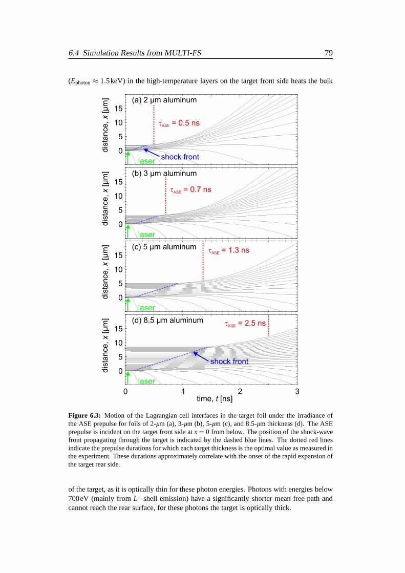
6.4 Simulation Results from MULTI-FS 79
(Ephoton≈ 1.5keV) in the high-temperature layers on the target front side heats the bulk
0
5
10
15
0
5
10
15
0
5
10
15
0
5
10
15
0 2 31time, [ns]t
dis
tan
ce
,[µ
m]
x(a) 2 µm aluminum
(b) 3 µm aluminum
(c) 5 µm aluminum
(d) 8.5 µm aluminum
laser
laser
laser
laser
dis
tan
ce
,[µ
m]
xd
ista
nce
,[µ
m]
xd
ista
nce
,[µ
m]
x
shock front
shock front
tASE = 2.5 ns
tASE = 1.3 ns
tASE = 0.7 ns
tASE = 0.5 ns
Figure 6.3: Motion of the Lagrangian cell interfaces in the target foil under the irradiance ofthe ASE prepulse for foils of 2-µm (a), 3-µm (b), 5-µm (c), and 8.5-µm thickness (d). The ASEprepulse is incident on the target front side atx = 0 from below. The position of the shock-wavefront propagating through the target is indicated by the dashed blue lines. The dotted red linesindicate the prepulse durations for which each target thickness is the optimal value as measured inthe experiment. These durations approximately correlate with the onset of the rapid expansion ofthe target rear side.
of the target, as it is optically thin for these photon energies. Photons with energies below700eV (mainly fromL−shell emission) have a significantly shorter mean free path andcannot reach the rear surface, for these photons the target is optically thick.
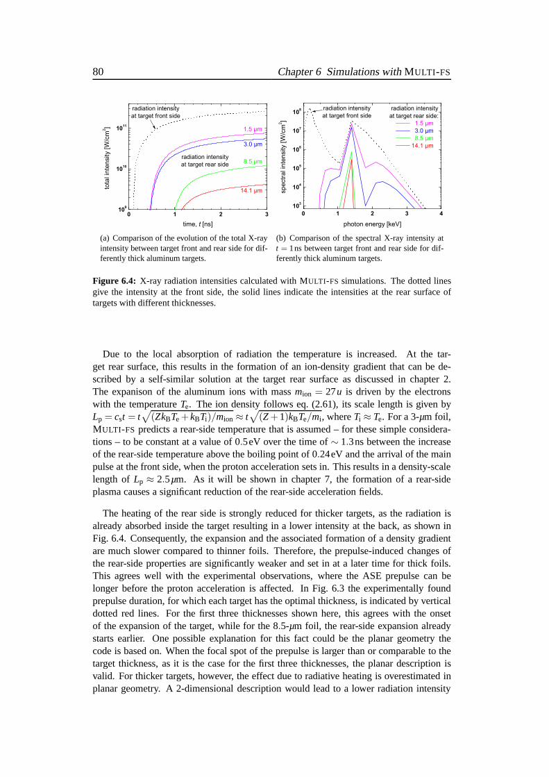
80 Chapter 6 Simulations withMULTI -FS
(a) Comparison of the evolution of the total X-rayintensity between target front and rear side for dif-ferently thick aluminum targets.
(b) Comparison of the spectral X-ray intensity att = 1ns between target front and rear side for dif-ferently thick aluminum targets.
Figure 6.4: X-ray radiation intensities calculated with MULTI -FS simulations. The dotted linesgive the intensity at the front side, the solid lines indicate the intensities at the rear surface oftargets with different thicknesses.
Due to the local absorption of radiation the temperature is increased. At the tar-get rear surface, this results in the formation of an ion-density gradient that can be de-scribed by a self-similar solution at the target rear surface as discussed in chapter 2.The expanison of the aluminum ions with massmion = 27u is driven by the electronswith the temperatureTe. The ion density follows eq. (2.61), its scale length is given byLp = cst = t
√
(ZkBTe+kBTi)/mion ≈ t√
(Z+1)kBTe/mi , whereTi ≈ Te. For a 3-µm foil,MULTI -FS predicts a rear-side temperature that is assumed – for thesesimple considera-tions – to be constant at a value of 0.5eV over the time of∼ 1.3ns between the increaseof the rear-side temperature above the boiling point of 0.24eV and the arrival of the mainpulse at the front side, when the proton acceleration sets in. This results in a density-scalelength of Lp ≈ 2.5µm. As it will be shown in chapter 7, the formation of a rear-sideplasma causes a significant reduction of the rear-side acceleration fields.
The heating of the rear side is strongly reduced for thicker targets, as the radiation isalready absorbed inside the target resulting in a lower intensity at the back, as shown inFig. 6.4. Consequently, the expansion and the associated formation of a density gradientare much slower compared to thinner foils. Therefore, the prepulse-induced changes ofthe rear-side properties are significantly weaker and set inat a later time for thick foils.This agrees well with the experimental observations, wherethe ASE prepulse can belonger before the proton acceleration is affected. In Fig. 6.3 the experimentally foundprepulse duration, for which each target has the optimal thickness, is indicated by verticaldotted red lines. For the first three thicknesses shown here,this agrees with the onsetof the expansion of the target, while for the 8.5-µm foil, the rear-side expansion alreadystarts earlier. One possible explanation for this fact could be the planar geometry thecode is based on. When the focal spot of the prepulse is largerthan or comparable to thetarget thickness, as it is the case for the first three thicknesses, the planar description isvalid. For thicker targets, however, the effect due to radiative heating is overestimated inplanar geometry. A 2-dimensional description would lead toa lower radiation intensity
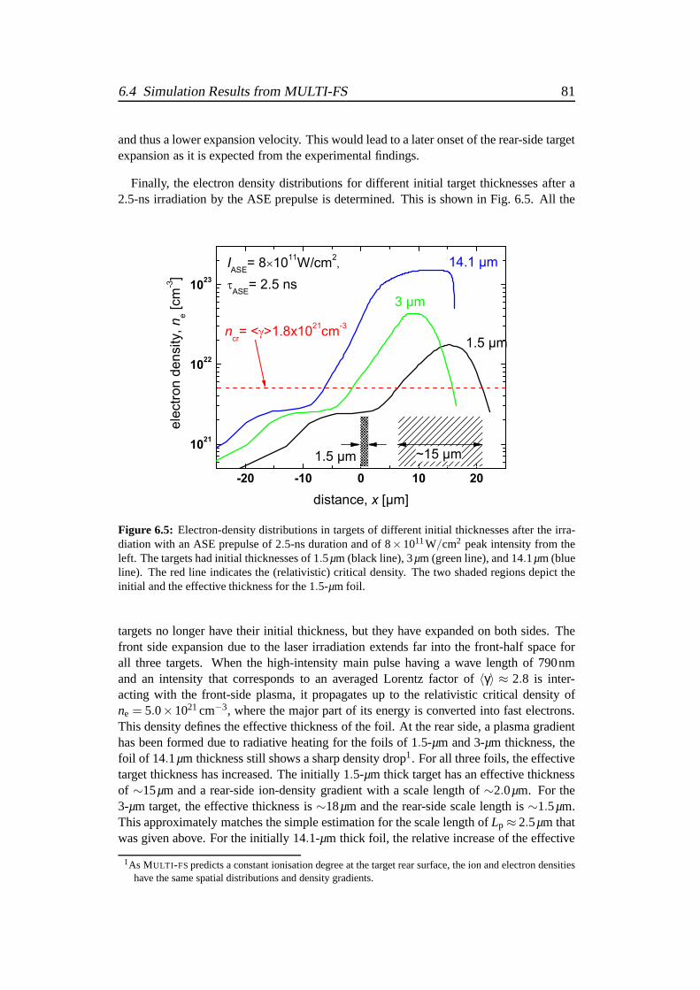
6.4 Simulation Results from MULTI-FS 81
and thus a lower expansion velocity. This would lead to a later onset of the rear-side targetexpansion as it is expected from the experimental findings.
Finally, the electron density distributions for differentinitial target thicknesses after a2.5-ns irradiation by the ASE prepulse is determined. This is shown in Fig. 6.5. All the
Figure 6.5: Electron-density distributions in targets of different initial thicknesses after the irra-diation with an ASE prepulse of 2.5-ns duration and of 8×10¹¹W/cm2 peak intensity from theleft. The targets had initial thicknesses of 1.5µm (black line), 3µm (green line), and 14.1µm (blueline). The red line indicates the (relativistic) critical density. The two shaded regions depict theinitial and the effective thickness for the 1.5-µm foil.
targets no longer have their initial thickness, but they have expanded on both sides. Thefront side expansion due to the laser irradiation extends far into the front-half space forall three targets. When the high-intensity main pulse having a wave length of 790nmand an intensity that corresponds to an averaged Lorentz factor of 〈γ〉 ≈ 2.8 is inter-acting with the front-side plasma, it propagates up to the relativistic critical density ofne = 5.0×1021cm−3, where the major part of its energy is converted into fast electrons.This density defines the effective thickness of the foil. At the rear side, a plasma gradienthas been formed due to radiative heating for the foils of 1.5-µm and 3-µm thickness, thefoil of 14.1µm thickness still shows a sharp density drop1. For all three foils, the effectivetarget thickness has increased. The initially 1.5-µm thick target has an effective thicknessof ∼15µm and a rear-side ion-density gradient with a scale length of∼2.0µm. For the3-µm target, the effective thickness is∼18µm and the rear-side scale length is∼1.5µm.This approximately matches the simple estimation for the scale length ofLp ≈ 2.5µm thatwas given above. For the initially 14.1-µm thick foil, the relative increase of the effective
1As MULTI -FSpredicts a constant ionisation degree at the target rear surface, the ion and electron densitieshave the same spatial distributions and density gradients.
82 Chapter 6 Simulations withMULTI -FS
thickness to∼22µm is much smaller and the rear-side gradient is much steeper with ascale length smaller than 0.2µm.
At the target front side, the electron density gradient depends only very weakly onthe target thickness. For all different thicknesses used inthe experiment, the front-sideelectron-density gradient varies between 3.5µm for the thickest foils and 4.5µm for the1.5-µm foil for the prepulse duration ofτASE = 2.5ns (these cases are shown in Fig. 6.5).For the shortest prepulse duration ofτASE = 0.5ns, MULTI -FS predicts a constant value of0.5µm for all target thicknesses. Furthermore, the position of the critical density is onlyshifted within≈ 15µm, what is below the Rayleigh length of the focusing optics. Thisstrongly suggests that the process of electron acceleration at the target front side remainsunaffectedfor a constant prepulse duration, when the target thickness is changed. Itmight change for different prepulse duration also leading to a different injection angleof the electron beam into the target, as it was discussed in chapter 2.2. This effect wasrecently observed in an ongoing experiment using the same laser system at MPQ [118].
6.5 Summary of the MULTI-FS Simulations
• The ASE prepulse impinging on the target heats up the front surface and increasesthe effective target thickness. A shock wave is launched into the target.
• Additionally, the target material is radiatively heated due to X-rays generated inthe focus of the prepulse. Due to the heating of the target rear side an ion-densitygradient is formed. The rear-side heating is strongly reduced for thicker targets dueto absorption of the radiation in the target. Furthermore, the relative increase of thetarget thickness due to the prepulse is much less pronouncedfor thicker foils.
• Assuming a cold and unexpanded target and a shock wave propagating with thesound speed of the cold material as in [37] is not sufficient toexplain our experi-mental observations, as in our experiments the shock wave istoo weak. Here, theradiative heating has to be taken into account.
• The front-side electron-density gradient remains almost constant for a fixed pre-pulse duration and all target thicknesses used in the experiments implying that theelectron acceleration remains unaffected for a scan of the target thicknesses with afixed value ofτASE.
Chapter 7
A One-Dimensional Simulation Code for theRear-Side Acceleration of Protons
In this chapter, a one-dimensional simulation code will be introduced that was newlydeveloped to describe the process of proton acceleration atthe target rear side. After adetailed description of the simulation code itself the validity of the analytical formulasderived in chapter 2 is shown and the effect of an initial proton-density gradient at thetarget rear side is investigated.
7.1 Description of the Simulation Code
The process of proton acceleration at the rear side of the target is described by meansof a 1-dimensional simulation code, that is based on a 1-D model by Crowet al. [84].Published in 1975, it was developed to describe the ion acceleration in laser-plasma inter-actions using ns-pulses, which were the shortest pulses available at that time.
The physical picture of the rear-side acceleration is the same, as it was already de-scribed in chapter 2. The gradient of the rear-side potential, which initiates the proton ac-celeration, depends on the initial density,ne0, and the temperature,Te, of the hot-electroncomponent, as it was shown in chapter 2. But furthermore, it depends on the initial densitydistribution of the protons at the rear side before the acceleration starts. The analyticalsolution derived in chapter 2 is valid for an initially step-like distribution only. The caseof a preformed plasma at the target rear surface having an exponential drop in the protondensity cannot be treated analytically. Such a case corresponds to a plasma formationdue to the prepulse-launched heat wave arriving at the back of the target. This case willtherefore be investigated using this simulation code. After the acceleration of the protonshas started, the proton distribution expands away from the target-rear surface, addition-ally affecting the gradient of the rear-side potential. Allthese effects are included in thesimulation, giving a detailed insight into the acceleration process.
83
84 Chapter 7 1-D Simulations for Rear-Side Proton Acceleration
7.1.1 Set of Equations Solved by the Code
The proton acceleration is described by the following set ofequations including the Pois-son equation, the equation of motion, and the equation of continuity for the protons:
ε0∂2Φel(x, t)
∂x2 = e[
ne(x, t)−np(x, t)]
, (7.1)
E(x, t) = − ∂∂x
Φel(x, t), (7.2)
∂vp(x, t)∂t
+vp(x, t)∂vp(x, t)
∂x=
emp
E(x, t), and (7.3)
∂np(x, t)
∂t+
∂∂x
[
np(x, t) ·vp(x, t)]
= 0. (7.4)
Here,Φel(x, t) is the potential andE(x, t) the electric field arising from the charge separa-tion, that is described by the electron and proton densities, ne(x, t) andnp(x, t). During theacceleration process the proton-velocity distribution,vp(x, t), changes. This set of equa-tions is integrated numerically at discrete times,tk, leading to new proton-density and-velocity distributions for the next time step,tk+1.
7.1.2 Initial Conditions
The acceleration of the protons, that is driven by the electrostatic field set up by the hotelectrons leaking out of the back of the target, is describedby the evolution of the densityand velocity distributions,np(x, t) andvp(x, t), of the protons. These quantities are numer-ically calculated at discrete time steps,tk, that are separated by a constant time interval,∆t. The electron distribution,ne(x, t), with an initial value,ne0, and a Boltzmann-liketemperature,Te, is assumed to be in thermal equilibrium with the electrostatic potential,Φel(x, t), for all times ttt ≥ 0 during the whole acceleration process:
ne(x, t) = ne0·exp
[
eΦel(x, t)kBTe
]
(7.5)
The initial proton distribution can either be step-like or it can drop exponentially witha characteristic density-scale length,Lp. The former situation is the same as it was in-troduced in chapter 2, the latter takes into account the effect of a rear-side expansion dueto the prepulse-induced shock wave. Beyondxmax(0), which is the initial position of theproton front before the acceleration starts, the density drops to 0:
np(x,0) =
ne0 for x≤ 0ne0·exp−x/Lp for 0≤ x≤ xmax(0)0 for xmax(0) < x.
(7.6)
As from the prepulse-induced plasma formation at the rear side, that acts over several100’s of ps or even ns, the effective energy gain of the protons is small compared to thesubsequent acceleration by the MeV-electrons, the protonsin the initial density profile areassumed to be at rest before the acceleration starts, i.e.vp(x,0) ≡ 0.

7.1 Description of the Simulation Code 85
7.1.3 Calculation of the Electrostatic Potential
At each time steptk ≥ 0, the electrostatic potential,Φel(x, tk), and the electron-densitydistribution,ne(x, tk), that is described by eq. (7.5), are obtained by numericallysolvingthe Poisson equation including the momentary proton-density distribution,np(x, tk). Thisnumerical integration, that is carried out over the distance, x, is devided into two parts.
First the Poisson equation
ε0∂2Φel(x, tk)
∂x2 = e
[
ne0·exp
[
eΦel(x, tk)kBTe
]
−np(x, tk)
]
(7.7)
is integrated in the region where both electrons and protonsare present starting from themomentary position of the proton front,xmax = xmax(tk), to x → −∞. As eq. (7.7) isa second-order differential equation, that does not dependon the first derivative of thepotential,∂Φel(x, tk)/∂x, Stoermer’s rule can be used for integration [119]. For thisin-tegration, the boundary conditions are not given at the position of the proton front,xmax,what would be necessary for the initialisation of the numerical integration. However, thepotential and the electric field have to vanish forx → −∞ to provide charge neutralityin the undisturbed plasma. A so-calledshooting methodis used to overcome this prob-lem [87, 119]. The initial value of the potential,Φel(xmax), that also determines the slopeof the potential,Φel
′(xmax), as it will be shown in a moment, is guessed and the numericalintegration is carried out. Depending on the behaviour ofΦel(x) for x → −∞ with theguessed value, the starting value of the potential is varied, until the left boundary condi-tions, i.e.Φel(x) → 0 andΦel
′(x) → 0 for x→−∞, are fulfilled. In the simulation, this isachieved with an accuracy of better than 10−7.
In the second step, the Poisson equation is solved forx≥ xmax(tk), where a pure electroncloud is present. Here the Poisson equation reads
ε0∂2Φel(x, t)
∂x2 = ene0·exp
[
eΦel(x, t)kBTe
]
. (7.8)
As the potential has to be continously differentiable at theproton front, the initial valuesfor the numerical integration in this second step hae to be the same as determined in thefirst step.
The two parts of the numerical solution together give the potential,Φel(x, tk), associatedto the electron and proton distributions at time,tk, at all positions,x. The electric field thatdrives the proton acceleration and changes the proton-density distribution during the nexttime step is finally obtained by
E(x, tk) = − ∂∂x
Φel(x, tk). (7.9)
Figure 7.1 shows the calculated electron densities (red line) and electric fields (dashedblue line in the lower plots) fort = 0 for a proton distribution (black line), that is initiallystep-like (a) and for one having an exponential drop in the density at the back of thetarget (b). In the simulation, a fully ionised hydrogen plasma is assumed having the samedensity as the hot electrons forx→−∞, thus assuring charge neutrality.

86 Chapter 7 1-D Simulations for Rear-Side Proton Acceleration
(a) Step-like proton-density (b) Exponential proton-density drop
Figure 7.1: Initial proton- and electron-density distributions and resulting electric fields at thetarget rear surface with no proton-density gradient (a) anda density gradient withLp = 0.8µm(b). The undisturbed density of the electron beam in the target is ne0 = 3.4×1020cm−3 with atemperature ofTe = 100keV. The resulting electric field that is peaked at the proton front issignificantly reduced in the case with a rear-side proton-density gradient (b), leading to lower finalenergies of the accelerated protons.
The numerical procedure that gives an accurate descriptionof the acceleration of theprotons follows in the next section.
7.1.4 Acceleration of the Proton Distribution
Calculation of the New Proton Velocity Distribution
To describe the acceleration of the protons that have a momentary density and velocitydistribution,np(x, tk) andvp(x, tk), during the next iterative time step,∆t, the distributionsare divided into cells of constant thickness,∆x, starting at the proton front,xmax(tk). Eachboundary between two cells at a position,x j , has a definite proton density and velocity.During ∆t, each boundary is moving due to the velocity,vp(x j , tk), and due to the accel-eration by the electric field,E(x j , tk), at this boundary position. This is described by theequation of motion of the protons and it is implemented into the code in the following
7.1 Description of the Simulation Code 87
way:
x j → x′j = x j +vp(x j , tk) ·∆t +e
2mpE(x j , tk) ·∆t2 (7.10)
vp(x j , tk) → vp(x′j , tk+1) = vp(x j , tk)+
emp
E(x j , tk) ·∆t (7.11)
The electric field is assumed to be constant over the distancethe protons move dur-ing the time interval, i.e., a constant force on the protons in a given cell is assumed.The new proton velocities,vp(x′j , tk+1), that were calculated at the new boundary posi-tions, x′j , at time tk+1 are used to obtain the new entire proton-velocity distribution bylinear interpolation. Note that due to the shift of each boundary the total derivative,dvp(x, t)/dt = ∂vp(x, t)/∂t +vp ·∂vp(x, t)/∂x in eq. (7.3) is taken into account.
Calculation of the New Proton Density Distribution
Due to the different proton velocities at the different cellboundaries, the width of eachcell changes. Assuming a constant total number of protons ineach cell, the proton densitychanges accordingly during∆t.
This is solved numerically in the following way, which is also sketched in Figure 7.2.If ∆x j and∆x′j are the thicknesses of a certain cell with the right boundaryat x j andx′j ,respectively, before and after one time interval, then the new density in the shifted cell is
np(x′j , tk+1) = np(x j , tk)
∆x j
∆x′j(7.12)
with the new cell thickness
∆x′j = x′j −x′j+1
= x j −x j+1 +[
vp(x j , tk)−vp(x j+1, tk)]
·∆t
+e
2mp[E(x j , tk)−E(x j+1, tk)] ·∆t2
= ∆x j + ∆v j ·∆t +e
2mp∆E j ·∆t2. (7.13)
The new densities are, similar to the new velocities, definedat the shifted position,x′j , ofthe right boundary. The entire proton-density distribution, np(x, tk+1), is again obtainedby linear interpolation.
7.1.5 Derivation of the Proton-Energy Spectrum
As the numerical simulation calculates the proton-densitydistribution, np(x, t), and theproton-velocity distribution,vp(x, t), the proton-energy spectrum, dnp/dEp, can also be
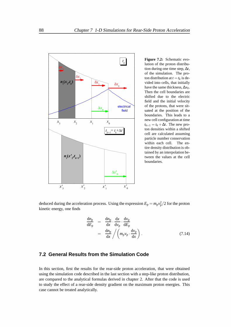
88 Chapter 7 1-D Simulations for Rear-Side Proton Acceleration
Figure 7.2: Schematic evo-lution of the proton distribu-tion during one time step,∆t,of the simulation. The pro-ton distribution att = tk is de-vided into cells, that initiallyhave the same thickness,∆x0.Then the cell boundaries areshifted due to the electricfield and the initial velocityof the protons, that were sit-uated at the position of theboundaries. This leads to anew cell configuration at timetk+1 = tk + ∆t. The new pro-ton densities within a shiftedcell are calculated assumingparticle number conservationwithin each cell. The en-tire density distribution is ob-tained by an interpolation be-tween the values at the cellboundaries.
deduced during the acceleration process. Using the expression Ep = mpv2p/2 for the proton
kinetic energy, one finds
dnp
dEp=
dnp
dx· dxdvp
· dvp
dEp
=dnp
dx
/(
mpvp ·dvp
dx
)
. (7.14)
7.2 General Results from the Simulation Code
In this section, first the results for the rear-side proton acceleration, that were obtainedusing the simulation code described in the last section witha step-like proton distribution,are compared to the analytical formulas derived in chapter 2. After that the code is usedto study the effect of a rear-side density gradient on the maximum proton energies. Thiscase cannot be treated analytically.
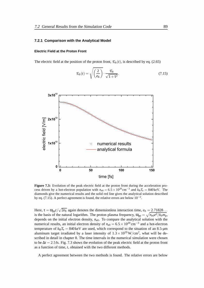
7.2 General Results from the Simulation Code 89
7.2.1 Comparison with the Analytical Model
Electric Field at the Proton Front
The electric field at the position of the proton front,Efr(t), is described by eq. (2.65)
Efr(t) =
√
(
2eE
)
· E0√1+ τ2
. (7.15)
Figure 7.3: Evolution of the peak electric field at the proton front during the acceleration pro-cess driven by a hot-electron population withne0 = 6.5×1020cm−3 andkBTe = 840keV. Thediamonds give the numerical results and the solid red line gives the analytical solution describedby eq. (7.15). A perfect agreement is found, the relative errors are below 10−2.
Here,τ = ωppt/√
2eE again denotes the dimensionless interaction time,eE = 2.71828. . .is the basis of the natural logarithm. The proton plasma frequency,ωpp =
√
ne0e2/ε0mp,depends on the initial electron density,ne0. To compare the analytical solution with thenumerical results, an initial electron density ofne0 = 6.5×1020cm−3 and a hot-electrontemperature ofkBTe = 840keV are used, which correspond to the situation of an 8.5-µmaluminum target irradiated by a laser intensity of 1.3×10¹⁹W/cm2, what will be de-scribed in detail in chapter 8. The time intervals in the numerical simulation were chosento be∆t = 2.5fs. Fig. 7.3 shows the evolution of the peak electric field atthe proton frontas a function of time,t, obtained with the two different methods.
A perfect agreement between the two methods is found. The relative errors are below
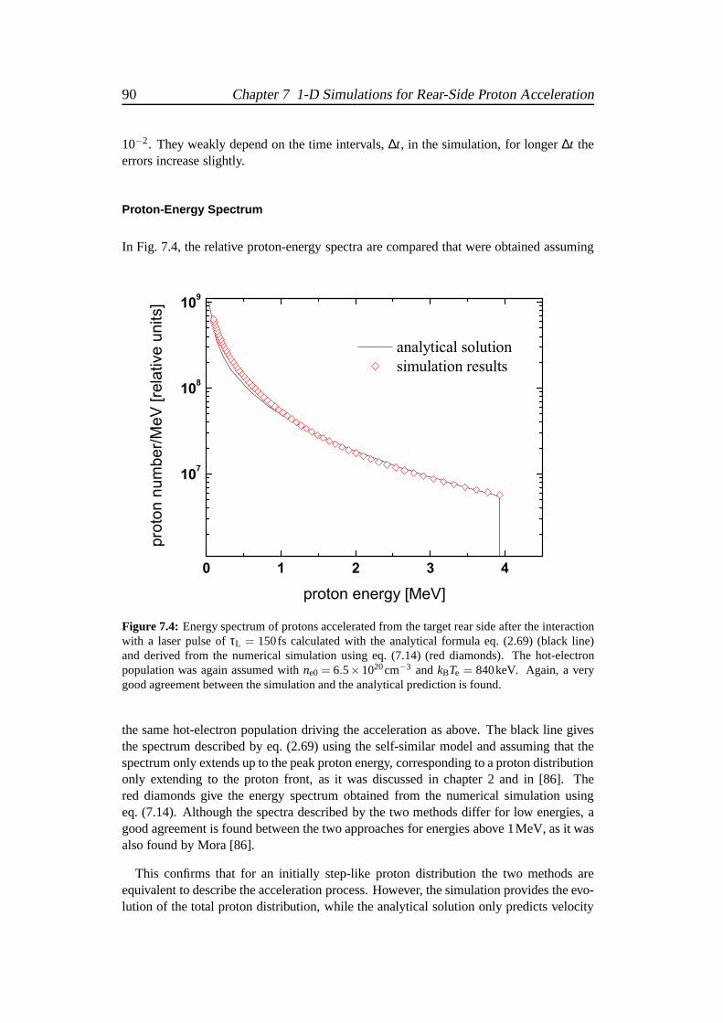
90 Chapter 7 1-D Simulations for Rear-Side Proton Acceleration
10−2. They weakly depend on the time intervals,∆t, in the simulation, for longer∆t theerrors increase slightly.
Proton-Energy Spectrum
In Fig. 7.4, the relative proton-energy spectra are compared that were obtained assuming
Figure 7.4: Energy spectrum of protons accelerated from the target rearside after the interactionwith a laser pulse ofτL = 150fs calculated with the analytical formula eq. (2.69) (black line)and derived from the numerical simulation using eq. (7.14) (red diamonds). The hot-electronpopulation was again assumed withne0 = 6.5×1020cm−3 andkBTe = 840keV. Again, a verygood agreement between the simulation and the analytical prediction is found.
the same hot-electron population driving the accelerationas above. The black line givesthe spectrum described by eq. (2.69) using the self-similarmodel and assuming that thespectrum only extends up to the peak proton energy, corresponding to a proton distributiononly extending to the proton front, as it was discussed in chapter 2 and in [86]. Thered diamonds give the energy spectrum obtained from the numerical simulation usingeq. (7.14). Although the spectra described by the two methods differ for low energies, agood agreement is found between the two approaches for energies above 1MeV, as it wasalso found by Mora [86].
This confirms that for an initially step-like proton distribution the two methods areequivalent to describe the acceleration process. However,the simulation provides the evo-lution of the total proton distribution, while the analytical solution only predicts velocity
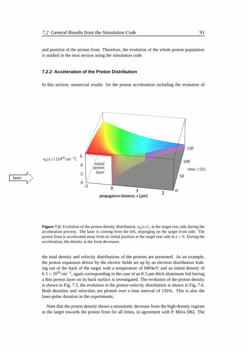
7.2 General Results from the Simulation Code 91
and position of the proton front. Therefore, the evolution of the whole proton populationis studied in the next section using the simulation code.
7.2.2 Acceleration of the Proton Distribution
In this section, numercial results
@@laser
for the proton acceleration including the evolution of
-1-1 00 11 22
0
2
4
6
0
50
100
150
propagation distance,x [µm]propagation distance,x [µm]
time, t [fs]
np(x,t) [1020cm−3]initial
protonlayer
Figure 7.5: Evolution of the proton density distribution,np(x,t), at the target rear side during theacceleration process. The laser is coming from the left, impinging on the target front side. Theproton front is accelerated away from its initial position at the target rear side atx = 0. During theacceleration, the density at the front decreases.
the total density and velocity distributions of the protonsare presented. As an example,the proton expansion driven by the electric fields set up by anelectron distribution leak-ing out of the back of the target with a temperature of 840keV and an initial density of6.5×1020cm−3, again corresponding to the case of an 8.5-µm thick aluminum foil havinga thin proton layer on its back surface is investigated. The evolution of the proton densityis shown in Fig. 7.5, the evolution ot the proton-velocity distribution is shown in Fig. 7.6.Both densities and velocities are plotted over a time interval of 150fs. This is also thelaser-pulse duration in the experiments.
Note that the proton density shows a monotonic decrease fromthe high-density regionsin the target towards the proton front for all times, in agreement with P. Mora [86]. The

92 Chapter 7 1-D Simulations for Rear-Side Proton Acceleration
peak in the proton-density distribution in the vicinity of the proton front, as it was ob-served in simulations carried out by Crowet al. [84] and other authors (see referencesin [86]), is not present in our simulations.
-1-1 00 11 22
0
1
2
3
0
50
100
150
propagation distance,x [µm]propagation distance,x [µm]
time, t [fs]vp(x,t) [107m/s]
Figure 7.6: Evolution of the proton velocity distribution,vp(x,t), during the acceleration pro-cess. The protons situated at the front are accelerated strongest and gain peak velocities of2.74×107m/s, i.e. 0.092× c, wherec is the velocity of light. This peak velocity correspondsto a kinetic proton energy of 3.93MeV.
7.2.3 Influence of an Initial Rear-Side Density Gradient
@@
laser
In this section, results from simulations carried out including an initial proton-densitygradient at the target rear surface are described. As already depicted in Fig. 7.1, such adensity gradient reduces the electric fields at the proton front. This can be explained asfollows. Although thetotal potential difference determined by the total charge separa-tion is the same, the potential drops over a larger distance as the charge distribution isdistributed over a larger area. Therefore thelocal gradient of the potential (which is thelocal electric field) is smaller compared to the case of an initially step-like proton dis-tribution. As the life-time of the fields driving the proton acceleration is limited by thelaser-pulse duration, the protons gain significantly lowerfinal energies, when the electric
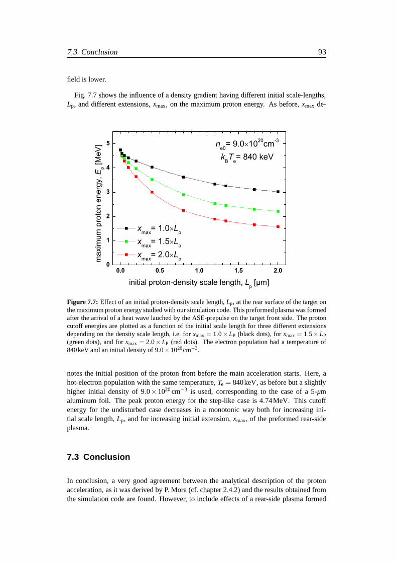
7.3 Conclusion 93
field is lower.
Fig. 7.7 shows the influence of a density gradient having different initial scale-lengths,Lp, and different extensions,xmax, on the maximum proton energy. As before,xmax de-
Figure 7.7: Effect of an initial proton-density scale length,Lp, at the rear surface of the target onthe maximum proton energy studied with our simulation code.This preformed plasma was formedafter the arrival of a heat wave lauched by the ASE-prepulse on the target front side. The protoncutoff energies are plotted as a function of the initial scale length for three different extensionsdepending on the density scale length, i.e. forxmax = 1.0×LP (black dots), forxmax = 1.5×LP
(green dots), and forxmax = 2.0× LP (red dots). The electron population had a temperature of840keV and an initial density of 9.0×1020cm−3.
notes the initial position of the proton front before the main acceleration starts. Here, ahot-electron population with the same temperature,Te = 840keV, as before but a slightlyhigher initial density of 9.0×1020cm−3 is used, corresponding to the case of a 5-µmaluminum foil. The peak proton energy for the step-like caseis 4.74MeV. This cutoffenergy for the undisturbed case decreases in a monotonic wayboth for increasing ini-tial scale length,Lp, and for increasing initial extension,xmax, of the preformed rear-sideplasma.
7.3 Conclusion
In conclusion, a very good agreement between the analyticaldescription of the protonacceleration, as it was derived by P. Mora (cf. chapter 2.4.2) and the results obtained fromthe simulation code are found. However, to include effects of a rear-side plasma formed

94 Chapter 7 1-D Simulations for Rear-Side Proton Acceleration
by the laser prepulse, numerical simulations are inevitable. The effect of this ion-densitygradient on the maximum proton energy accelerated from the target rear side appears tobe too large to be negligible.
In the next chapter, the experimental results of the proton energies are compared to thepredictions obtained with the simulation code, that was described in this chapter. Further-more, the prepulse-induced changes in the target properties, as they were simulated byMULTI -FS (cf. chapter 6), will be included.

Chapter 8
Discussion of the Experimental Results
This chapter discusses the experimental results presentedin chapter 5 and gives quanti-tative explanations of the results by the comparison with different numerical simulationsthat were introduced in chpater 6 and chapter 7. In the first two sections, the results ob-tained from the thickness scan are compared to two differentscenarios for the transport ofthe electron beam through the target, one assuming a free-streaming propagation and theother including electron-transport effects arising from the collective behaviour of the elec-trons, as it was discussed in chapter 2.3. In the last section, the results obtained from theangularly-resolved measurements are compared to 3-dimensional PIC simulations [45].
8.1 Results from the Target-Thickness Scan Explained by a“Free-Streaming” Electron-Propagation Model
In this section, a simple quantitative explanation for the experimental results concerningthe proton acceleration obtained during the scans of the target thickness is found. Forthis purpose, both the 1-D simulation code introduced in chapter 7 to describe the protonacceleration at the target rear side and the analytical theory introduced in chapter 2 for thefront-side acceleration are used. The necessary parameters for the numerical simulationare the rear-side electron density,ne0, the hot-electron temperature,Te, and the interactiontime, t. In a first step, afree-streamingelectron beam in the target is assumed to derivethese initial parameters.
8.1.1 Approximations for the Assumption of a Free-Streamin g ElectronBeam
The approximations made in this scenario are as follows. Theelectrons are acceleratedwithin the laser-focal spot on the front side and propagate normally through the targetforming a cone-shaped electron beam.
• The cone formed by the electron beam has a constant divergence, characterised byan initial half opening angle,θin.
95
96 Chapter 8 Discussion of the Experimental Results
• When the electrons exit the target at the rear side, they still have the same averagedkinetic energy as on the target front side, given by their quasi-temperature,kBTe.
• The total number of hot electrons in the beam remains constant during its passagethrough the target.
• The electron pulse length is assumed to be equal to the laser pulse duration.
The simulations were carried out using the experimental parameters. The ATLAS laser,that was described in detail in chapter 3.1, delivers pulsesof 150-fs duration (FWHM)and of 790-nm wavelength. The total energy on the target amounts toEL = 600. . .850mJ,resulting in an averaged laser intensity,IL , between 1.0 and 1.5×10¹⁹W/cm2 within afocal spot ofrf = 2.6µm radius, as it was discussed in chapter 3.2.
Determination of the Initial Simulation Parameters
The hot-electron temperature,Te, is calculated from the averaged laser intensity using theponderomotive scaling law by Wilkset al., eq. (2.44)
kBTe = 0.511MeV·
√
1+ILλL
2
1.37×10¹⁸W/cm2 ·µm2−1
. (8.1)
The electron density at the target rear surface,ne0, is derived from the total numberof electrons,Ne, the focal-spot size on the front side, the target thickness, dtarget, and theinitial half-opening angle,θin. Again, it is assumed that a fraction ofη = 25% of thelaser energy,EL, is converted into hot electrons [9] with a mean energy determined by thehot-electron temperature given by eq. (8.1). This gives a total electron number of
Ne ≈ηEL
kBTe. (8.2)
These electrons are emitted in a cone-shaped beam that transverses the target and has atotal length ofcτL , determined by the laser pulse duration, if the velocity of the electrons,ve ≈ c, and dispersion effects due to different electron velocities are neglected. This alsodetermines the electron pulse duration and the rear-side acceleration time tot = τL .
The radius of the electron spot at the rear side of the target can be deduced from simplegeometrical considerations assuming a constant divergence of the beam. This is sketchedin Fig. 8.1. Starting with a minimal cross section of the beamat the target front side,which is determined by the focal-spot size of the laser, the cross section increases whilethe electrons propagate through the target. Depending on the injection angle,αin, of theelectron beam into the target that depends on the electron acceleration mechanism on thetarget front side, the effective thickness of the target through which the electron beam hasto propagate is given byd∗
target= dtarget/cos(αin). The radius of the rear-side electron spotis then approximately given by(rf + d∗
t tanθin). This determines the electron density atthe rear surface to
ne0≈Ne
cτL ×π(rf +d∗targettanθin)2 . (8.3)
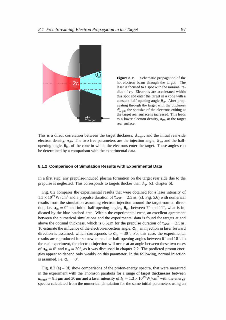
8.1 Free-Streaming Electron Propagation in the Target 97
2rf
d*target
qin Figure 8.1: Schematic propagation of the
hot-electron beam through the target. Thelaser is focused to a spot with the minimal ra-dius of rf . Electrons are accelerated withinthis spot and enter the target in a cone with aconstant half-opening angleθin. After prop-agating through the target with the thicknessd∗
target, the spotsize of the electrons exiting atthe target rear surface is increased. This leadsto a lower electron density,ne0, at the targetrear surface.
This is a direct correlation between the target thickness,dtarget, and the initial rear-sideelectron density,ne0. The two free parameters are the injection angle,αin, and the half-opening angle,θin, of the cone in which the electrons enter the target. These angles canbe determined by a comparison with the experimental data.
8.1.2 Comparison of Simulation Results with Experimental D ata
In a first step, any prepulse-induced plasma formation on thetarget rear side due to theprepulse is neglected. This corresponds to targets thickerthandopt (cf. chapter 6).
Fig. 8.2 compares the experimental results that were obtained for a laser intensity of1.3×1019W/cm2 and a prepulse duration ofτASE = 2.5ns, (cf. Fig. 5.6) with numericalresults from the simulation assuming electron injection around the target-normal direc-tion, i.e. αin = 0 and initial half-opening angles,θin, between 7 and 11, what is in-dicated by the blue-hatched area. Within the experimental error, an excellent agreementbetween the numerical simulations and the experimental data is found for targets at andabove the optimal thickness, which is 8.5µm for the prepulse duration ofτASE = 2.5ns.To estimate the influence of the electron-incection angle,αin, an injection in laser forwarddirection is assumed, which corresponds toαin = 30. For this case, the experimentalresults are reproduced for somewhat smaller half-opening angles between 6 and 10. Inthe real experiment, the electron injection will occur at anangle between these two casesof αin = 0 andαin = 30, as it was discussed in chapter 2.2. The predicted proton ener-gies appear to depend only weakly on this parameter. In the following, normal injectionis assumed, i.e.αin = 0.
Fig. 8.3 (a) – (d) show comparisons of the proton-energy spectra, that were measuredin the experiment with the Thomson parabola for a range of target thicknesses betweendtarget= 8.5µm and 30µm and a laser intensity ofIL = 1.3×10¹⁹W/cm2 with the energyspectra calculated from the numerical simulation for the same initial parameters using an

98 Chapter 8 Discussion of the Experimental Results
Figure 8.2: Comparison between the maximum proton energy,Ep, obtained in the experimentwith a laser intensity of 1.3×10¹⁹W/cm2, a prepulse duration of 2.5ns, and different targetthicknesses,dtarget, and the cutoff energies,Ep,rear, obtained from the numerical simulation forthe rear-side acceleration. Normal injection of the electron beam was assumed,αin = 0, and arange of half-opening angles,θin, between 7 and 11. This area is hatched in blue.
initial half-opening angle ofθin = 9. As it can be seen in the plots, also the proton-energyspectra are well reproduced by the simulation in terms of cutoff energy and temperature,but only for the hottest proton component. The cold proton component in the spectrum,that is not reproduced by the simulation for any foil thickness, can either come froma second, colder component in theelectron-energy spectrum, as it has been observedexperimentally by L. M. Wickenset al. [120] and explained theoretically by J. Denavit[85], or it indicates that the rear-side acceleration is notthe only active mechanism. Thispoint will be addressed below.
In Fig. 8.4, the results for the proton cutoff energies obtained from the numericalsimulation are compared to the experimental data for a slightly lower laser intensity ofIL = 1.0×10¹⁹W/cm2, as it was present in the experiment. This plot contains the re-sults for three different ASE prepulse durations. For eachτASE, a very good agreementbetween experiment and simulation is found at and above theindividual optimal targetthickness depending on the prepulse duration (dopt = 2µm for τASE = 0.5ns,dopt = 3µmfor τASE = 0.7ns, anddopt = 8.5µm for τASE = 2.5ns). Below each individual optimaltarget thickness, the proton cutoff energies remain well below the theoretical prediction.In this range, the experimental observations cannot be explained by the simple modelassuming an initially step-like proton distribution at thetarget rear side.
As it was shown in chapter 6, the values for the optimal targetthickness are qualita-
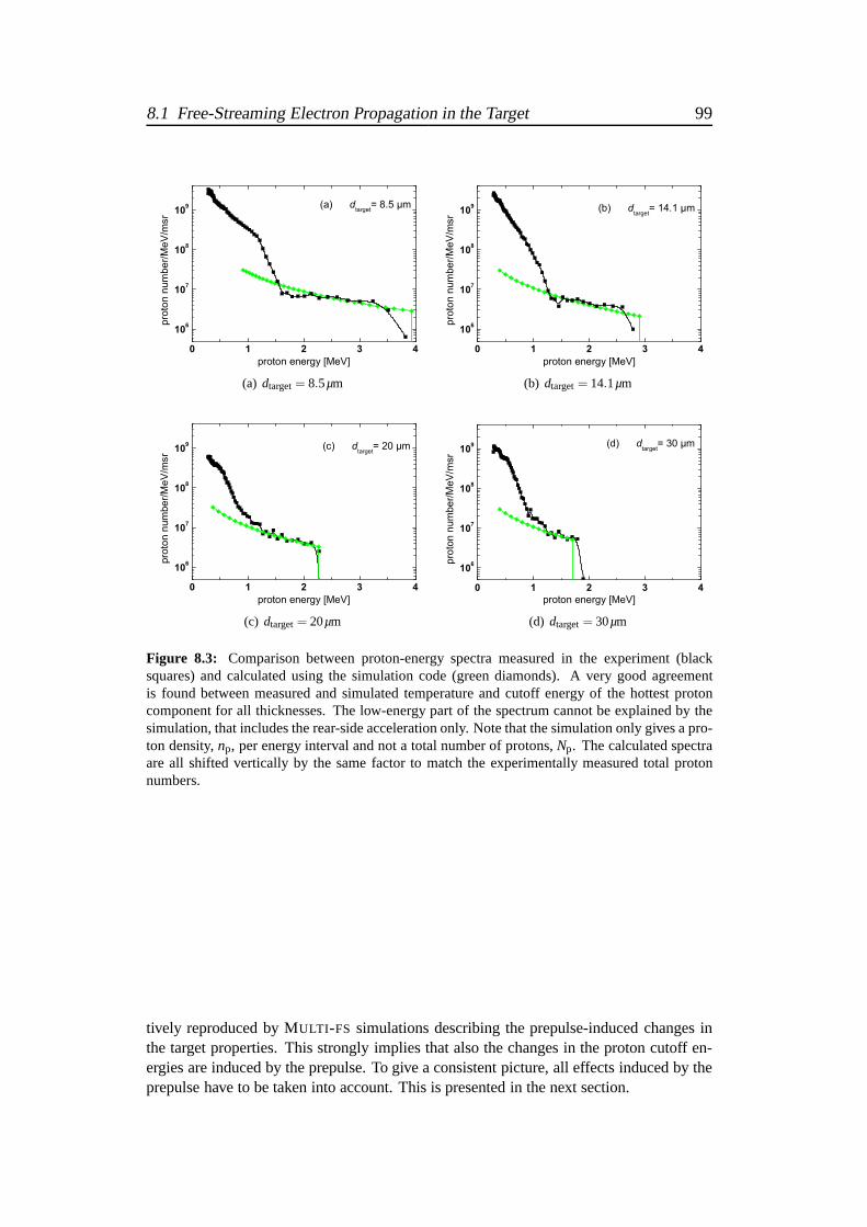
8.1 Free-Streaming Electron Propagation in the Target 99
(a) dtarget= 8.5µm (b) dtarget= 14.1µm
(c) dtarget= 20µm (d) dtarget= 30µm
Figure 8.3: Comparison between proton-energy spectra measured in the experiment (blacksquares) and calculated using the simulation code (green diamonds). A very good agreementis found between measured and simulated temperature and cutoff energy of the hottest protoncomponent for all thicknesses. The low-energy part of the spectrum cannot be explained by thesimulation, that includes the rear-side acceleration only. Note that the simulation only gives a pro-ton density,np, per energy interval and not a total number of protons,Np. The calculated spectraare all shifted vertically by the same factor to match the experimentally measured total protonnumbers.
tively reproduced by MULTI -FS simulations describing the prepulse-induced changes inthe target properties. This strongly implies that also the changes in the proton cutoff en-ergies are induced by the prepulse. To give a consistent picture, all effects induced by theprepulse have to be taken into account. This is presented in the next section.

100 Chapter 8 Discussion of the Experimental Results
Figure 8.4: Comparison between maximum proton energies from the experiment and from thesimulation for a laser intensity of 1.0×10¹⁹W/cm2, three different prepulse durations of 0.5ns,0.7ns, and 2.5ns, and different target thicknesses,dtarget. Again a good agreement between experi-ment and theory is found but only for targets at and above theindividualoptimal target thicknesses,that depend on the individual prepulse durations. Note thatexactly the same range of initial half-opening angles (7 ≤ θin ≤ 11) was used for the simulation as in Fig. 8.2.
8.2 Prepulse-Induced Effects Relevant for the Rear-Side Pr otonAcceleration: Numerical Description of the Fast-ElectronTransport
In the last section, the “free-streaming” model for the electron propagation in the targetwas used to interprete the experimental results concerningthe rear-side proton accelera-tion.
A more elaborated picture should additionally include the prepulse-induced changes ofthe target properties as density and temperature variations, and describe their influenceon the proton acceleration. The rear-side proton acceleration is directly influenced by theformation of an ion-density gradient at the target rear side, as it was shown in chapter 7.Furthermore, one would expect that the expansion as well as the associated density andtemperature variations inside the target influence the electron transport through the mate-rial, too. This indirectly influences the proton acceleration, as the latter depends on theelectron density distribution at the rear side of the target, which is likely to be modifiedby the electron transport.

8.2 Relevance of Electron-Transport Effects for Proton Acceleration 101
To include all these aspects, numerical simulations with a fast-electron transport (FET)code were carried out by J. J. Honrubia. This code calculatesthe density distributionsand mean energies of the electrons exiting the target at the rear side. These values areused afterwards in the numerical simulation code for the rear-side proton acceleration,that was described in chapter 7, where also the rear-side density distribution influencingthe proton acceleration can be taken into account. This finally yields the peak proton ener-gies including all prepulse induced effects, which are thencompared to the experimentalresults.
8.2.1 The Fast-Electron Transport Code
The FET code is a hybrid code. While the fast electrons are described as “macro” parti-cles each representing a fixed number of 106 “real” electrons as in a PIC code, the coldbackground electrons are treated as a fluid. It describes thepropagation of a relativisticelectron population through a target that can exhibit any initial ion- and electron-densitydistribution. These initial target properties are calculated separately by MULTI -FS or anequivalent hydro code, simulating the influence of the laserprepulse on an aluminum foilof a given thickness as described in chapter 6. The return current induced by the fastelectron current is computed self-consistently, including the heating of the backgroundplasma due to resistive heating of the return current and dueto energy deposition by col-lisions. These collisions are treated as in standard 3-D Monte-Carlo codes. Additionally,the formation of azimuthal magnetic fields is calculated. These fields can pinch the fastelectron beam as a whole.
The electromagnetic fields are calculated by combining Ampere’s law without displace-ment current [121] with the simplest form of Ohm’s law and Faraday’s law
~jr = −~jf +1µ0
~∇×~B, (8.4)
~E =1σ·~jr, and (8.5)
∂~B∂t
= −~∇×~E , (8.6)
where~jf and~jr are the fast and return current densities, respectively, and σ = 1/η is thetarget conductivity,η is the resistivity, both depending on the background ion density andthe temperature (see below). In the code, the particle trajectories are simulated in 3-D,but to describe the electromagnetic field generation in the target, cylindrical symmetryaround the axis of the injected electron beam is assumed. Therefore, the code takes intoaccount the electric fields in radial and longitudinal direction, Er andEx, respectively, andthe azimuthal magnetic fields,Bθ. These fields are generated during the the propagationof the electron beam. To provide charge neutrality, a returncurrent sets in immediatelyafter the onset of the electron-beam injection as describedby eq. (8.4). The conductivityof aluminum is computed by the model of Lee and More [122], which allows to calculatetransport properties of partially degenerated plasmas. The conductivity of aluminum fordifferent temperatures and two different densities is depicted in Fig. 8.5. Note that theconductivity for low densities, i.e. for an expanded targetwith temperatures below 100eV,
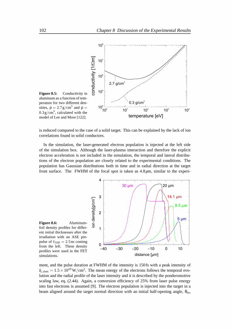
102 Chapter 8 Discussion of the Experimental Results
Figure 8.5: Conductivity inaluminum as a function of tem-perature for two different den-sities, ρ = 2.7g/cm3 andρ =
0.3g/cm3, calculated with themodel of Lee and More [122].
2.7 g/cm3
conductivity [1/
m]
W
temperature [eV]
108
107
106
104
105
104
103
102
101
100
0.3 g/cm3
is reduced compared to the case of a solid target. This can be explained by the lack of ioncorrelations found in solid conductors.
In the simulation, the laser-generated electron population is injected at the left sideof the simulation box. Although the laser-plasma interaction and therefore the explicitelectron acceleration is not included in the simulation, the temporal and lateral distribu-tions of the electron population are closely related to the experimental conditions. Thepopulation has Gaussian distributions both in time and in radial direction at the targetfront surface. The FWHM of the focal spot is taken as 4.8µm, similar to the experi-
Figure 8.6: Aluminum-foil density profiles for differ-ent initial thicknesses after theirradiation with an ASE pre-pulse ofτASE = 2.5ns comingfrom the left. These densityprofiles were used in the FETsimulations.
30 µm 20 µm
14.1 µm
8.5 µm
5 µm
distance [µm]
ion d
ensity[g
/cm
]3
ment, and the pulse duration at FWHM of the intensity is 150fswith a peak intensity ofIL,max = 1.5×10¹⁹W/cm2. The mean energy of the electrons follows the temporal evo-lution and the radial profile of the laser intensity and it is described by the ponderomotivescaling law, eq. (2.44). Again, a conversion efficiency of 25% from laser pulse energyinto fast electrons is assumed [9]. The electron populationis injected into the target in abeam aligned around the target normal direction with an initial half-opening angle,θin,
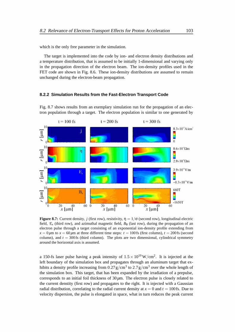
8.2 Relevance of Electron-Transport Effects for Proton Acceleration 103
which is the only free parameter in the simulation.
The target is implemented into the code by ion- and electron density distributions anda temperature distribution, that is assumed to be initially1-dimensional and varying onlyin the propagation direction of the electron beam. The ion-density profiles used in theFET code are shown in Fig. 8.6. These ion-density distributions are assumed to remainunchanged during the electron-beam propagation.
8.2.2 Simulation Results from the Fast-Electron Transport Code
Fig. 8.7 shows results from an exemplary simulation run for the propagation of an elec-tron population through a target. The electron population is similar to one generated by
Figure 8.7: Current density,j (first row), resistivity,η = 1/σ (second row), longitudinal electricfield, Ex (third row), and azimuthal magnetic field,Bθ (last row), during the propagation of anelectron pulse through a target consisting of an exponential ion-density profile extending fromx = 0µm to x = 60µm at three different time steps:t = 100fs (first column),t = 200fs (secondcolumn), andt = 300fs (third column). The plots are two dimensional, cylindrical symmetryaround the horizontal axis is assumed.
a 150-fs laser pulse having a peak intensity of 1.5×10¹⁹W/cm2. It is injected at theleft boundary of the simulation box and propagates through an aluminum target that ex-hibits a density profile increasing from 0.27g/cm3 to 2.7g/cm3 over the whole length ofthe simulation box. This target, that has been expanded by the irradiation of a prepulse,corresponds to an initial foil thickness of 30µm. The electron pulse is closely related tothe current denstity (first row) and propagates to the right.It is injected with a Gaussianradial distribution, correlating to the radial current density atx = 0 andt = 100fs. Due tovelocity dispersion, the pulse is elongated in space, what in turn reduces the peak current
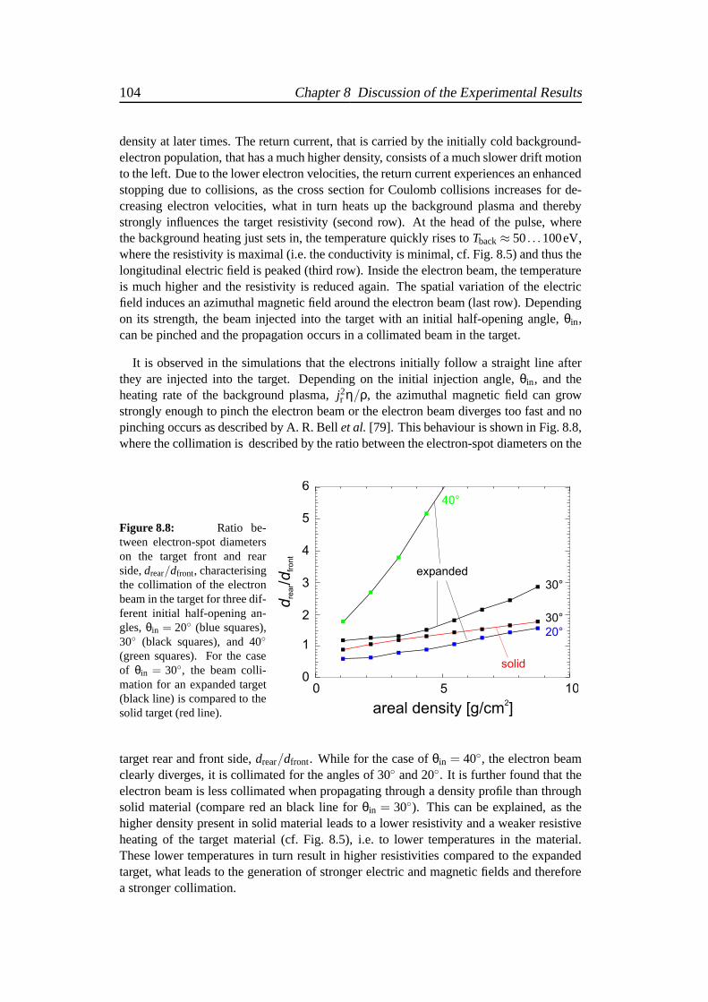
104 Chapter 8 Discussion of the Experimental Results
density at later times. The return current, that is carried by the initially cold background-electron population, that has a much higher density, consists of a much slower drift motionto the left. Due to the lower electron velocities, the returncurrent experiences an enhancedstopping due to collisions, as the cross section for Coulombcollisions increases for de-creasing electron velocities, what in turn heats up the background plasma and therebystrongly influences the target resistivity (second row). Atthe head of the pulse, wherethe background heating just sets in, the temperature quickly rises toTback≈ 50. . .100eV,where the resistivity is maximal (i.e. the conductivity is minimal, cf. Fig. 8.5) and thus thelongitudinal electric field is peaked (third row). Inside the electron beam, the temperatureis much higher and the resistivity is reduced again. The spatial variation of the electricfield induces an azimuthal magnetic field around the electronbeam (last row). Dependingon its strength, the beam injected into the target with an initial half-opening angle,θin,can be pinched and the propagation occurs in a collimated beam in the target.
It is observed in the simulations that the electrons initially follow a straight line afterthey are injected into the target. Depending on the initial injection angle,θin, and theheating rate of the background plasma,j2r η/ρ, the azimuthal magnetic field can growstrongly enough to pinch the electron beam or the electron beam diverges too fast and nopinching occurs as described by A. R. Bellet al.[79]. This behaviour is shown in Fig. 8.8,where the collimation is described by the ratio between the electron-spot diameters on the
Figure 8.8: Ratio be-tween electron-spot diameterson the target front and rearside,drear/dfront, characterisingthe collimation of the electronbeam in the target for three dif-ferent initial half-opening an-gles,θin = 20 (blue squares),30 (black squares), and 40
(green squares). For the caseof θin = 30, the beam colli-mation for an expanded target(black line) is compared to thesolid target (red line). areal density [g/cm ]
2
dd
rear
front
/
40°
30°
30°
20°
expanded
solid
target rear and front side,drear/dfront. While for the case ofθin = 40, the electron beamclearly diverges, it is collimated for the angles of 30 and 20. It is further found that theelectron beam is less collimated when propagating through adensity profile than throughsolid material (compare red an black line forθin = 30). This can be explained, as thehigher density present in solid material leads to a lower resistivity and a weaker resistiveheating of the target material (cf. Fig. 8.5), i.e. to lower temperatures in the material.These lower temperatures in turn result in higher resistivities compared to the expandedtarget, what leads to the generation of stronger electric and magnetic fields and thereforea stronger collimation.
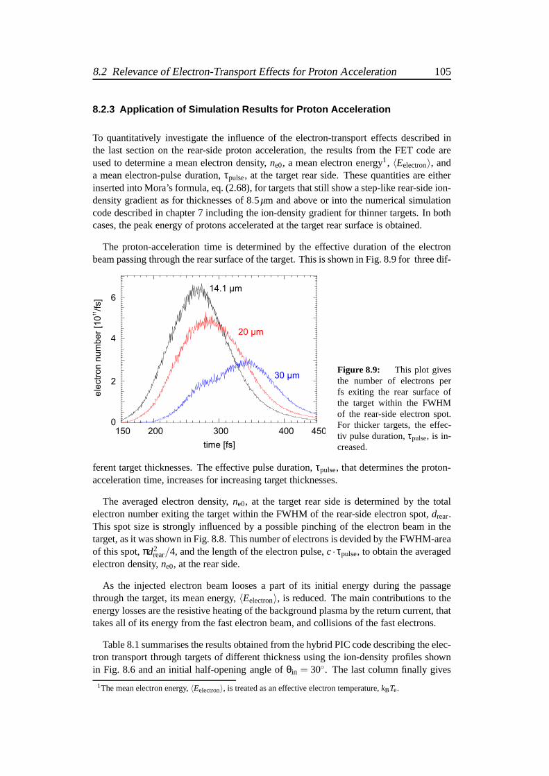
8.2 Relevance of Electron-Transport Effects for Proton Acceleration 105
8.2.3 Application of Simulation Results for Proton Acceler ation
To quantitatively investigate the influence of the electron-transport effects described inthe last section on the rear-side proton acceleration, the results from the FET code areused to determine a mean electron density,ne0, a mean electron energy1, 〈Eelectron〉, anda mean electron-pulse duration,τpulse, at the target rear side. These quantities are eitherinserted into Mora’s formula, eq. (2.68), for targets that still show a step-like rear-side ion-density gradient as for thicknesses of 8.5µm and above or into the numerical simulationcode described in chapter 7 including the ion-density gradient for thinner targets. In bothcases, the peak energy of protons accelerated at the target rear surface is obtained.
The proton-acceleration time is determined by the effective duration of the electronbeam passing through the rear surface of the target. This is shown in Fig. 8.9 for three dif-
ele
ctr
on n
um
ber
[10
/fs]
11
time [fs]
30 µm
20 µm
14.1 µm
Figure 8.9: This plot givesthe number of electrons perfs exiting the rear surface ofthe target within the FWHMof the rear-side electron spot.For thicker targets, the effec-tiv pulse duration,τpulse, is in-creased.
ferent target thicknesses. The effective pulse duration,τpulse, that determines the proton-acceleration time, increases for increasing target thicknesses.
The averaged electron density,ne0, at the target rear side is determined by the totalelectron number exiting the target within the FWHM of the rear-side electron spot,drear.This spot size is strongly influenced by a possible pinching of the electron beam in thetarget, as it was shown in Fig. 8.8. This number of electrons is devided by the FWHM-areaof this spot,πd2
rear/4, and the length of the electron pulse,c· τpulse, to obtain the averagedelectron density,ne0, at the rear side.
As the injected electron beam looses a part of its initial energy during the passagethrough the target, its mean energy,〈Eelectron〉, is reduced. The main contributions to theenergy losses are the resistive heating of the background plasma by the return current, thattakes all of its energy from the fast electron beam, and collisions of the fast electrons.
Table 8.1 summarises the results obtained from the hybrid PIC code describing the elec-tron transport through targets of different thickness using the ion-density profiles shownin Fig. 8.6 and an initial half-opening angle ofθin = 30. The last column finally gives
1The mean electron energy,〈Eelectron〉, is treated as an effective electron temperature,kBTe.

106 Chapter 8 Discussion of the Experimental Results
target thickness drear Nelectron τpulse 〈Eelectron〉 Eproton
(µm) (µm) (×1011) (fs) (MeV) (MeV)1.5 4.6 7.30 185 0.65 0.93 (1.94)2 4.3 6.42 190 0.67 1.02 (2.05)3 3.8 5.38 190 0.69 1.15 (2.22)5 4.8 4.93 175 0.75 2.66 (3.72)
8.5 5.0 5.35 180 0.75 3.8714.1 6.2 5.81 180 0.75 3.1320 7.4 5.15 205 0.73 2.4630 7.6 3.00 220 0.72 1.68
Table 8.1: Parameters for the rear-side proton acceleration obatinedfrom the hybrid PIC simu-lation. Here, the ion density profiles from Fig. 8.6 and an initial half-opening angle ofθin = 30
were used. The last column gives the peak proton energy as predicted by Mora’s analytical for-mula, eq. (2.68) or by the numerical proton simulation. For the first four thicknesses, the energyin brackets gives the proton energy for a step-like ion density distribution at the target rear side.The reduced energy takes into account the effect of the prepulse-induced rear-side gradient.
the proton cutoff energies that were calculated either withMora’s formula, eq. (2.68), orwith the numerical simulation for the rear-side acceleration. For the first four thicknesses
Figure 8.10: This plot compares the simulated proton cutoff energies from three different modelswith the experimental data (red squares).
(dtarget≤ 5µm), the two different energy values correspond to the cases (i) including anion-density gradient, the scale length of which was predicted by MULTI -FS, or (ii) a step-like ion density distribution. The density gradient leads to a significantly reduced protoncutoff energy, as it was also shown in chapter 7 and has to be taken into account. These
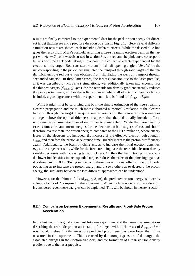
8.2 Relevance of Electron-Transport Effects for Proton Acceleration 107
results are finally compared to the experimental data for thepeak proton energy for differ-ent target thicknesses and a prepulse duration of 2.5ns in Fig. 8.10. Here, several differentsimulation results are shown, each including different effects. While the dashed blue linegives the result from Mora’s formula assuming a free-streaming electron beam in the tar-get withθin = 9, as it was discussed in section 8.1, the red and the pink curvecorrespondto runs with the FET code taking into account the collective effects experienced by theelectrons in the target. Both runs start with an initial half-opening angle of 30. While therun corresponding to the pink curve simulated the transportthrough solid targets of the ini-tial thickness, the red curve was obtained from simulating the electron transport through“expanded targets”. In these latter cases, the target expansion due to the laser prepulse,as it was described by MULTI -FS simulations, was additionally taken into account. Forthe thinnest targets (dtarget≤ 5µm), the the rear-side ion-density gradient strongly reducesthe peak proton energies. For the solid red curve, where all effects discussed so far areincluded, a good agreement with the experimental data is found for dtarget≥ 5µm.
While it might first be surprising that both the simple estimation of the free-streamingelectron propagation and the much more elaborated numerical simulation of the electrontransport through the target give quite similar results forthe rear-side proton energiesat targets above the optimal thickness, it appears that the additionally included effectsin the numerical simulation cancel each other to some extent. While the free-streamingcase assumes the same mean energies for the electrons on bothtarget surfaces and shouldtherefore overestimate the proton energies compared to theFET simulation, where energylosses of the electrons are included, the increase of the effective electron pulse length,τpulse, and therefore the proton acceleration time, slightly increase the proton cutoff energyagain. Additionally, the beam pinching acts as to increase the initial electron densities,ne0, at the target rear side, while for the free-streaming case the rear-side electron densitysteadily decreases with increasing target thickness. On the other hand, taking into accountthe lower ion densities in the expanded targets reduces the effect of the pinching again, asit is shown in Fig. 8.10. Taking into account these four additional effects in the FET code,two acting as to increase the proton energy and the two othersas to decrease the protonenergy, the similarity between the two different approaches can be understood.
However, for the thinnest foils (dtarget≤ 3µm), the predicted proton energy is lower byat least a factor of 2 compared to the experiment. When the front-side proton accelerationis considered, even those energies can be explained. This will be shown in the next section.
8.2.4 Comparison between Experimental Results and Front-S ide ProtonAcceleration
In the last section, a good agreement between experiment andthe numerical simulationsdescribing the rear-side proton acceleration for targets with thicknesses ofdtarget≥ 5µmwas found. Below this thickness, the predicted proton energies were lower than thosemeasured in the experiment. This is caused by the strong expansion of the target, theassociated changes in the electron transport, and the formation of a rear-side ion-densitygradient due to the laser prepulse.

108 Chapter 8 Discussion of the Experimental Results
However, including the front-side acceleration mechanismgives a natural explanationfor this feature. The peak energies of protons, that are accelerated on the target front sideby the electric fields set up by the ponderomotive charge-separation in the laser focus,depend on the laser intensity only. The initial energies canbe described by eq. (2.53)
Ep,front = 1.15MeV·(√
1+ILλ2
L
1.37×10¹⁸W/cm2 ·µm2−1
)
, (8.7)
that was derived in chapter 2. For the three laser intensities corresponding to the differentlines in Fig. 5.6, this formula leads to front-side peak proton energies of
Ep,front = 1.56MeV for IL = 1.0×10¹⁹W/cm2,
Ep,front = 1.87MeV for IL = 1.3×10¹⁹W/cm2, and
Ep,front = 2.07MeV for IL = 1.5×10¹⁹W/cm2.
When protons of these kinetic energies propagate through are finally stopped. This stopping-
(a) IL = 1.0×10¹⁹W/cm2 (b) IL = 1.3×10¹⁹W/cm2
(c) IL = 1.5×10¹⁹W/cm2
Figure 8.11: Comparison between peakproton energies accelerated from the tar-get front side, that are subsequentlyslowed down in the target material(dashed green lines), and the experimen-tal measurements for three different laserintensities. For the shaded region encom-passing thin targets, the experimental datais well explained by the front-side ac-celeration mechanism, while the rear-sidemechanism predicts proton energies thatare too low.
mechanism is treated numerically using tabulated values for the stopping power, dE/dx,

8.2 Relevance of Electron-Transport Effects for Proton Acceleration 109
for protons in (cold) aluminum from the National Institute of Standards and Technology(NIST, [106]). The kinetic energy of the protons at a given depth, x, of the target isobtained by the following integration:
Ep(x) = Ep,front−x∫
0
∣
∣
∣
∣
dE(x′)dx′
∣
∣
∣
∣
dx′. (8.8)
The integration is carried out, until the proton is stopped.This stopping distance dependson the initial energy. In Fig. 8.11 the proton energies are shown that were calculated byassuming that the protons are accelerated at the target front side to a peak energy given byeq. (8.7) using the intensity from the experiment. When theypropagate through the targetmaterial they lose a part of their energy and would leave a target of a certain thicknesswith the kinetic energy given by the dashed green line.
A good agreement between the theoretical model for thefront-sideacceleration and theexperimental data is found for the thinnest foils and long prepulses, while in this region,the model for therear-sideacceleration including prepulse effects predicts peak protonenergies, that are too low compared to the experiment. On theother hand, the front-sideacceleration cannot explain the maximum proton energies atand above the optimal targetthickness, as their initial energy is too low and for thickertargets, the stopping in the targetmaterial reduces their kinetic energy even more.
8.2.5 Conclusions from the Target-Thickness Scan
Including all the prepulse-induced effects and considering the two different accelerationmechanisms from both target surfaces, the experimental data could well be reproducedby numerical and theoretical predictions. This is summarised in Fig. 8.12. It showsthe comparison between the experimentally measured protoncutoff energies for a laserintensity ofIL = 1.5×10¹⁹W/cm2 and the theoretically determined values using the twomodels for the front- and rear-side acceleration. The agreement between these modelsand different parts of the experimental curve suggests thatboth acceleration mechanismshave to be taken into account to explain the whole experiment.
The results from the comparison of the experimental data from the target-thicknessscans with numerical simulations considering all prepulse-induced effects can be sum-marised as follows:
• The occurance of the optimal target thickness for the protonacceleration,dopt, andits dependence on the prepulse duration,τASE, could be explained for the first timeby combining MULTI -FS simulations, that describe the influence of the laser pre-pulse due to ASE on the target properties, with a fast-electron transport code. Forsufficiently thin targets, the prepulse has both reduced thetarget density and formeda rear-side ion-density gradient. The first effect leads to aless collimated electrontransport in the target, as the collimating magnetic fields are weaker for lower tar-get densities. This reduces the electron density in the rear-side sheath. The lattereffect further reduces the acceleration fields as describedin chapter 7.2.3. Both
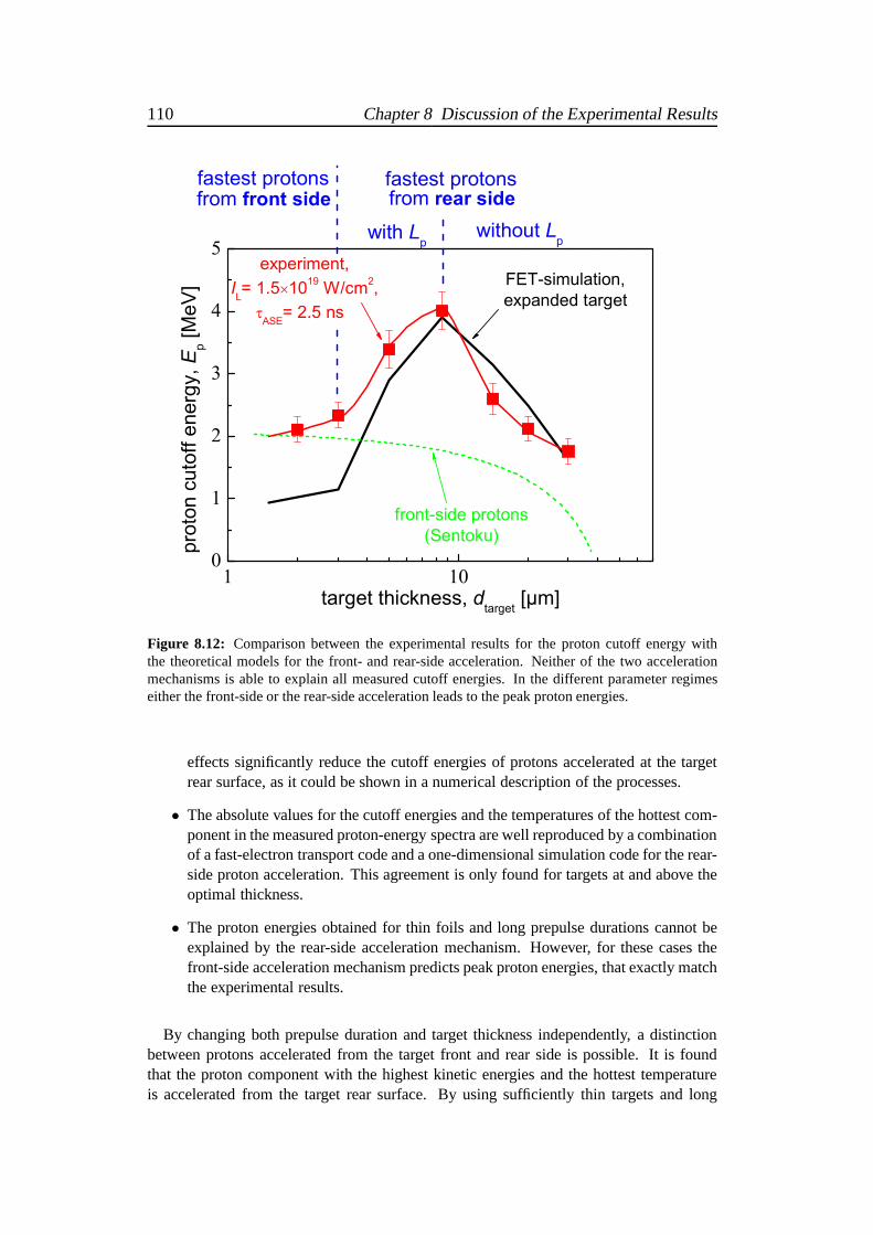
110 Chapter 8 Discussion of the Experimental Results
Figure 8.12: Comparison between the experimental results for the protoncutoff energy withthe theoretical models for the front- and rear-side acceleration. Neither of the two accelerationmechanisms is able to explain all measured cutoff energies.In the different parameter regimeseither the front-side or the rear-side acceleration leads to the peak proton energies.
effects significantly reduce the cutoff energies of protonsaccelerated at the targetrear surface, as it could be shown in a numerical descriptionof the processes.
• The absolute values for the cutoff energies and the temperatures of the hottest com-ponent in the measured proton-energy spectra are well reproduced by a combinationof a fast-electron transport code and a one-dimensional simulation code for the rear-side proton acceleration. This agreement is only found for targets at and above theoptimal thickness.
• The proton energies obtained for thin foils and long prepulse durations cannot beexplained by the rear-side acceleration mechanism. However, for these cases thefront-side acceleration mechanism predicts peak proton energies, that exactly matchthe experimental results.
By changing both prepulse duration and target thickness independently, a distinctionbetween protons accelerated from the target front and rear side is possible. It is foundthat the proton component with the highest kinetic energiesand the hottest temperatureis accelerated from the target rear surface. By using sufficiently thin targets and long

8.3 Results Obtained from the Angular Scan 111
prepulses, the generation of this component in the energy spectrum can be suppressed.In this case, only the proton component accelerated from thetarget front side remains,having a significantly colder temperature and lower peak energies.
8.3 Results Obtained from the Angular Scan
In chapter 5.4, angularly resolved measurements of the proton-energy spectra were shown.The proton-beam divergence was found to strongly depend on the kinetic energy of theprotons. Generally speaking, the low-temperature component in the proton spectrumshows a much smaller divergence, i.e. it is emitted in a very narrow cone, while the hot-temperature component is emitted in a cone with a significantly larger opening angle. Adetailed investigation presented in Fig. 5.12 revealed an energy dependence of the beamdivergence, that is peaked atEp ≈ 1.8. . .2MeV. Above this energy, the divergence angledecreases again what is in good agreement with measurementsfrom other groups [28,82].Furthermore, it was found that the strong collimation of thecold-proton component is re-duced for a longer prepulse duration.
These experimental findings will be explained by comparing the experimental resultswith 3-D particle-in-cell (PIC) simulations carried out byA. Pukhov [45] using the codeVLPL (the Virtual Laser Plasma Laboratory) [123].
8.3.1 Description of the Proton Acceleration with 3-D PIC co des
The entire process of proton acceleration from the target rear surface has to be treatedin two or even three dimensions. Although it is sufficient to describe the accelerationin 1D for the highest proton energies, that are accelerated in the center of the electronspot on the target rear side, where both temperature and hot-electron density are maximal[18,45,86], the slower protons are likely to be acceleratedfrom regions outside the centerof the electron sheath. This phenomenon has been observed byA. Pukhov in 3-D PICsimulations. In a numerical run simulating a “model problem” [45], a laser pulse of1-µm wave length and an intensity of 1019W/cm2 interacts with a 12-µm thick hydrogen-plasma layer with an initial electron density of 16×ncr.
The electrons accelerated at the target front side propagate through the target forminga cone that is characterised by its half-opening angle,θin, as described in the last section.These electrons leave the target and are pulled back by the arising electric fields thatalso drive the proton acceleration. As it has been observed in [45], the electrons forma “fountain”-like structure, while they are pulled back, what leads to a large halo in theelectron density around the dense spot, where the electronsfirst exit the target. When theseelectrons return to the target front surface, where they areagain pulled back into the targetand come back to the rear side a second time, as it has been described by A. Mackinnonand Y. Sentoku [38], they loose energy, while they heat up thebulk of the target, andquickly spread out sideways further increasing the electron-spot size on the rear side. Thehot-electron density distribution calculated from this simulation run is given in Fig. 8.13.

112 Chapter 8 Discussion of the Experimental Results
Figure 8.13: Electron density in the target in units ofncr = 1.1×1021cm−3 calculated byA. Pukhov [45]. The laser with an intensity ofIL = 1019W/cm2 and a wave length ofλ = 1µmimpinges on the left side of the target atx = 0 andy = 0 and accelerates electrons that propagatethrough the target several times. In this plot, the density distribution of electrons with kineticenergies above 100keV is shown after the laser pulse has terminated. These electrons form a“fountain”-like structure at the target rear side.
As a consequence of the fountain structure, the electron density remains as high asestimated in eq. (8.3) only in the center of the electron spotand quickly drops towards theouter regions where according to eq. (2.58) also the electric field is significantly lower.
Figure 8.14: 3-D view of the elec-trostatic field driving the proton accelera-tion calculated in 3-D PIC simulations in[45]. The blue isosurface has a field valueof −1.6×10¹¹V/m, the light red isosurfacecorresponds to 1.6×10¹¹V/m, and the darkred blob in the center has peak values of3.2×1011V/m.
This leads to a spatial distribution of the electric field, asit was calculated in [45] andshown in Fig. 8.14. Note that the center of the electron spot at the target rear side, wherethe electric field has its peak value, has a diameter of only∼ 10µm. This is in very goodagreement with the assumption for the half-opening angle,θin=(9±2) of the electronbeam in the target made in section 8.1.1, that predicts an electron-spot with a diameterof (8.8±0.9)µm for a target thickness of 12µm as it is simulated here and also with theresults from the FET code, where a diameter between 10µm and 12.4µm was predicted
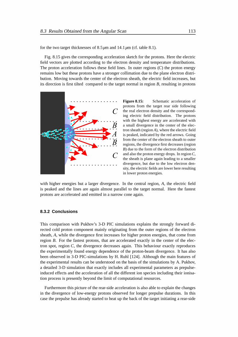
8.3 Results Obtained from the Angular Scan 113
for the two target thicknesses of 8.5µm and 14.1µm (cf. table 8.1).
Fig. 8.15 gives the corresponding acceleration sketch for the protons. Here the electricfield vectors are plotted according to the electron density and temperature distributions.The proton acceleration follows these field lines. In outer regions (C) the proton energyremains low but these protons have a stronger collimation due to the plane electron distri-bution. Moving towards the center of the electron sheath, the electric field increases, butits direction is first tilted compared to the target normal inregionB, resulting in protons
AB
B
C
C
Figure 8.15: Schematic acceleration ofprotons from the target rear side followingthe real electron density and the correspond-ing electric field distribution. The protonswith the highest energy are accelerated witha small divergence in the center of the elec-tron sheath (regionA), where the electric fieldis peaked, indicated by the red arrows. Goingfrom the center of the electron sheath to outerregions, the divergence first decreases (regionB) due to the form of the electron distributionand also the proton energy drops. In regionC,the sheath is plane again leading to a smallerdivergence, but due to the low electron den-sity, the electric fields are lower here resultingin lower proton energies.
with higher energies but a larger divergence. In the centralregion,A, the electric fieldis peaked and the lines are again almost parallel to the target normal. Here the fastestprotons are accelerated and emitted in a narrow cone again.
8.3.2 Conclusions
This comparison with Pukhov’s 3-D PIC simulations explainsthe strongly forward di-rected cold proton component mainly originating from the outer regions of the electronsheath,A, while the divergence first increases for higher proton energies, that come fromregionB. For the fastest protons, that are accelerated exactly in the center of the elec-tron spot, regionC, the divergence decreases again. This behaviour exactly reproducesthe experimentally found energy dependence of the proton-beam divergence. It has alsobeen observed in 3-D PIC-simulations by H. Ruhl [124]. Although the main features ofthe experimental results can be understood on the basis of the simulations by A. Pukhov,a detailed 3-D simulation that exactly includes all experimental parameters as prepulse-induced effects and the acceleration of all the different ion species including their ionisa-tion process is presently beyond the limit of computationalresources.
Furthermore this picture of the rear-side acceleration is also able to explain the changesin the divergence of low-energy protons observed for longerprepulse durations. In thiscase the prepulse has already started to heat up the back of the target initiating a rear-side

114 Chapter 8 Discussion of the Experimental Results
expansion that also has to be treated in 2-D, when regions outof the center of the electronspot are taken into account. Then the rear surface is no longer plane but has a convexshape. This leads to a larger divergence also for the low energy protons, in accordancewith the experimental observations.

Chapter 9
Summary and Perspectives
During the course of this thesis, experiments were carried out to characterise the proton-acceleration processes that are active during the interaction of high-intensity laser pulseswith solid targets. As a whole, the results and their theoretical interpretation answer manyquestions concerning the physics underlying the acceleration processes.
The results presented here shed new light onto experimentalparameters that were foundto have a profound effect on the proton acceleration. Together with laser intensity andpulse energy, the target thickness and the duration of the intrinsic prepulse due to ampli-fied spontaneous emission (ASE) were shown to play an important role. Within this work,the occurance of an optimal target thickness was observed and an explanation for its oc-curance was found. The value of the optimal thickness strongly depends on the prepulseduration that could for the first time both be controlled and varied.
The prepulse-induced changes of the target-density and -temperature distributions werefound to significantly influence the electron transport inside the target and as a conse-quence also the proton acceleration. Including these prepulse-changed target propertiesin computer simulations yielded a good agreement between the numerically predictedproton energies and the experimental data. However, the peak energies obtained forallexperimental parameters could only be explained by a physical picture that includes bothfront-side and rear-side acceleration mechanisms for protons.
It was found that the optimal target thickness delimits two proton acceleration regimes.At and above the optimal target thickness, the fastest protons are accelerated from the rearside, the electron beam propagating through the target is collimated in this regime. Forthinner targets, the density in the target is significantly reduced by the prepulse heating,what reduces the collimation of the electron beam in the target and consequently the rear-side acceleration fields. The latter are additionally diminished by an ion-density gradientthat was formed at the target rear side. By a further reduction of the target thickness therear-side mechanism is rendered more and more ineffective.The front-side mechanism,however, only depends on the laser intensity. For the thinnest targets and the longestprepulse durations, the rear-side acceleration is strongly suppressed and the fastest protonscome from the target front side.
The changes at the target rear surface are mainly induced by radiative heating due toprepulse-generated X-rays. This depends on the target thickness, as the radiation gener-ated in the focus of the prepulse on the target front side is the more absorbed inside the
115

116 Chapter 9 Summary and Perspectives
target the thicker it is. For thicker targets it was found that these changes of the targetproperties begin at a later time compared to thinner foils. This exactly reproduces theexperimental findings.
In conclusion, the experimental results and their theoretical and numerical interpre-tation reported in this thesis bring about new and relevant aspects concerning the laser-induced acceleration of protons and light ions for future experiments. They can also helpto understand and solve apparent discrepancies in the comparison of experiments that havebeen carried out with different laser systems. It turns out that is is of extreme importanceto control the laser prepulse – or at least characterise its temporal evolution – in order tootimise the experimental conditions for proton acceleration.
9.1 Possible Future Experiments on Proton Acceleration
This work has shown that also small-scale table-top laser systems as ATLAS have thepotential to be an efficient source of laser-accelerated protons, when all experimentalparameters including the prepulse duration can be controlled as accurately as possible. Itwas shown that it is preferable to reduce the laser prepulse to durations as short as possibleto maintain an undisturbed target rear surface also for the thinnest foils.
The MULTI -FS simulations describing the influence of the laser prepulse on the targetproperties have shown that for prepulse intensities as low as in the experiments describedhere the radiative heating is the dominant process to destroy the target rear surface beforethe main pulse arrives at the target front side and the rear-side proton acceleration isinitiated. One possibility to reduce this heating is to put avery thin low-Z layer on thefront side of the aluminum target that was used here. For sucha target configuration,the material of the front layer is also heated by the prepulsebut it emits characteristicradiation at lower photon energies compared to the aluminum. This radiation is quicklyabsorbed in the aluminum layer, leaving the target rear sideundisturbed. The layer onthe target front side (e.g. plastic or beryllium) should be as thin as possible to leave theelectron transport unaffected but thick enough to prevent the aluminum from heating bythe prepulse. Other high-Z materials as gold or tungsten could be used for the secondlayer, too.
Following the road towards shorter and shorter laser-pulsedurations, the applicabilityof such pulses for proton acceleration has to be addressed, too. The effectivity of therear-side acceleration mainly scales with the product of laser intensity and pulse duration,IL · τL , which is proportional to the laser energy,EL, if an optimal focusability of thelaser pusle is assumed. This relation was empirically foundby M. Roth by comparing allexisting results from different laser systems [125] with pulse durations ofτL ≤ 1ps. Thisdependency implies to use lasers with as high pulse energiesas possible for an efficientproton acceleration and not to reduce the pulse duration as much as possible. However,with lasers potentially delivering pulses as short as 5fs and peak intensities in excessof 1020 or even 1021W/cm2, the generation of electron populations having temperaturesin the range of 10MeV and high total numbers is possible. These electron populationsmight generate significantly stronger electric fields at therear side of the target and field-
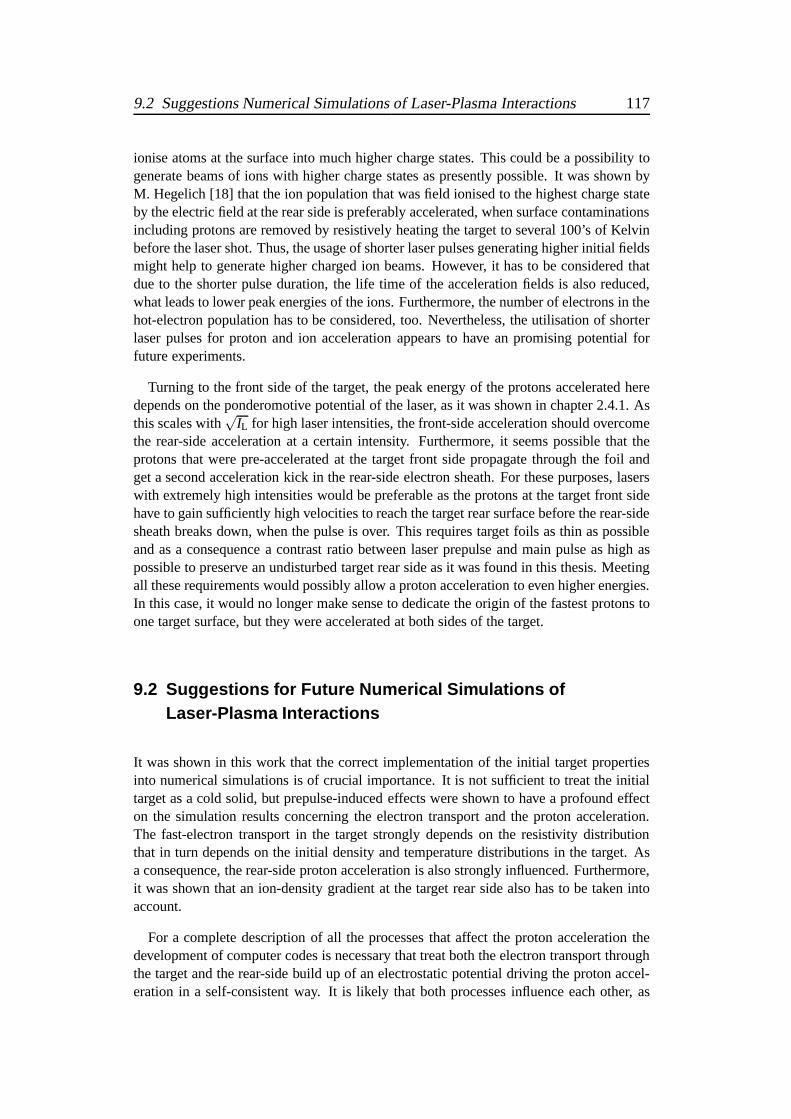
9.2 Suggestions Numerical Simulations of Laser-Plasma Interactions 117
ionise atoms at the surface into much higher charge states. This could be a possibility togenerate beams of ions with higher charge states as presently possible. It was shown byM. Hegelich [18] that the ion population that was field ionised to the highest charge stateby the electric field at the rear side is preferably accelerated, when surface contaminationsincluding protons are removed by resistively heating the target to several 100’s of Kelvinbefore the laser shot. Thus, the usage of shorter laser pulses generating higher initial fieldsmight help to generate higher charged ion beams. However, ithas to be considered thatdue to the shorter pulse duration, the life time of the acceleration fields is also reduced,what leads to lower peak energies of the ions. Furthermore, the number of electrons in thehot-electron population has to be considered, too. Nevertheless, the utilisation of shorterlaser pulses for proton and ion acceleration appears to havean promising potential forfuture experiments.
Turning to the front side of the target, the peak energy of theprotons accelerated heredepends on the ponderomotive potential of the laser, as it was shown in chapter 2.4.1. Asthis scales with
√IL for high laser intensities, the front-side acceleration should overcome
the rear-side acceleration at a certain intensity. Furthermore, it seems possible that theprotons that were pre-accelerated at the target front side propagate through the foil andget a second acceleration kick in the rear-side electron sheath. For these purposes, laserswith extremely high intensities would be preferable as the protons at the target front sidehave to gain sufficiently high velocities to reach the targetrear surface before the rear-sidesheath breaks down, when the pulse is over. This requires target foils as thin as possibleand as a consequence a contrast ratio between laser prepulseand main pulse as high aspossible to preserve an undisturbed target rear side as it was found in this thesis. Meetingall these requirements would possibly allow a proton acceleration to even higher energies.In this case, it would no longer make sense to dedicate the origin of the fastest protons toone target surface, but they were accelerated at both sides of the target.
9.2 Suggestions for Future Numerical Simulations ofLaser-Plasma Interactions
It was shown in this work that the correct implementation of the initial target propertiesinto numerical simulations is of crucial importance. It is not sufficient to treat the initialtarget as a cold solid, but prepulse-induced effects were shown to have a profound effecton the simulation results concerning the electron transport and the proton acceleration.The fast-electron transport in the target strongly dependson the resistivity distributionthat in turn depends on the initial density and temperature distributions in the target. Asa consequence, the rear-side proton acceleration is also strongly influenced. Furthermore,it was shown that an ion-density gradient at the target rear side also has to be taken intoaccount.
For a complete description of all the processes that affect the proton acceleration thedevelopment of computer codes is necessary that treat both the electron transport throughthe target and the rear-side build up of an electrostatic potential driving the proton accel-eration in a self-consistent way. It is likely that both processes influence each other, as

118 Chapter 9 Summary and Perspectives
those electrons, that have left the target, are pulled back by the arising electrostatic fieldat the rear side, and re-enter the target, modify the transport of those fast electrons thatfollow subsequently. This modification of the electron transport in turn has consequencesfor the rear-side acceleration. The development of such a code including all these effectsis currently under way [126].

Appendix A
Setup of a Novel Synchronised 2-ColourProbe Beam for Preplasma Diagnostic
In laser-plasma experiments, it is convenient to use probe beams synchronised to the mainpulse to backlight the laser-target interaction area from the side to record snapshots of thisarea with a time resolution that is given by the probe-beam duration (see e.g. [37,42,72]).By changing the delay between the main pulse and this probe beam on the target, theplasma evolution can be studied in a sequence of laser shots.In this appendix, we willdescribe the setup of a novel 2-colour probe beam that was used to study the generationand evolution both of preformed plasmas and of a plasma superchannel. With the noveltechnique using two probe beams, the formation state of the channel can be observed attwo different time stages during the very same laser shot.
After a short description of the setup in section A.1, the generation of two probe beamsof ∼150-fs duration and different wave lengths separated by∆t = 4.1ps is describedin section A.2. These two beams are used to probe a preplasma that was formed bya synchronised frequency-doubled Nd:Glass-laser delivering pulses of 12-J of energy at532-nm wave length with a duration of 3ns. Using a Wollaston prism for interferome-try [127], that is introduced in section A.3, the electron density of the preplasma can bededuced from these interferograms, as shown in section A.4.Finally, the formation of aplasma channel is observed [10, 72, 128], that is generated by focusing the synchronisedTi:sapphire-laser ATLAS into the preformed plasma.
A.1 Experimental Setup
The probe-beam setup is sketched in Fig. A.1. After the first multi-pass amplifier, apart of the streched beam is split off, recompressed to 130fsin the ATLAS-2 grating-compressor chamber and sent into a delay line. This 790-nm pulse contains∼ 5mJ ofenergy. After that the beam diameter is reduced by a lens telescope. This 1ω-beamis frequency doubled in a 2-mm thick type-1 KDP crystal. Before the pulse enters thecrystal, its polarisation is rotated by aλ/2 wave plate, that its plane of polarisation istilted by 45 to the vertical axis. The 2ω-pulse generated in the KDP crystal has its planeof polarisation rotated by 90 to the fundamental beam. This choice of polarisations wasnecessary for the interferometry using a Wollaston prism, what will be described below.These two beams are guided into the target chamber where theyboth pass the interaction
119
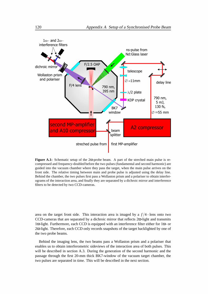
120 Appendix A Setup of a Synchronised Probe Beam
F/2.5 OAP
F/4 lens
Wollaston prismand polariser
second MP-amplifierand A10 compressor
A2 compressor
BK7window
delay line
telescope
790 nm,395 nm
ns-pulse fromNd:Glass laser
streched pulse from first MP-amplifier
KDP crystal
dichroic mirror
1 and 2
interference filters
w- w-
beamsplitter
790 nm,5 mJ,130 fs,
55 mmÆ =
Æ =11mm
l/2 plate
Figure A.1: Schematic setup of the 2ω-probe beam. A part of the streched main pulse is re-compressed and frequency-doubled before the two pulses (fundamental and second harmonic) areguided into the vacuum chamber where they pass the target, when the main pulse arrives on thefront side. The relative timing between main and probe pulseis adjusted using the delay line.Behind the chamber, the two pulses first pass a Wollaston prism and a polariser to obtain interfer-ograms of the interaction area, and finally they are separated by a dichroic mirror and interferencefilters to be detected by two CCD-cameras.
area on the target front side. This interaction area is imaged by a f/4−lens onto twoCCD-cameras that are separated by a dichroic mirror that reflects 2ω-light and transmits1ω-light. Furthermore, each CCD is equipped with an interference filter either for 1ω- or2ω-light. Therefore, each CCD only records snapshots of the target backlighted by one ofthe two probe beams.
Behind the imaging lens, the two beams pass a Wollaston prismand a polariser thatenables us to obtain interferometric sideviews of the interaction area of both pulses. Thiswill be described in section A.3. During the generation of the second harmonic and thepassage through the first 20-mm thick BK7-window of the vacuum target chamber, thetwo pulses are separated in time. This will be described in the next section.

A.2 Generation of two fs-Probe Beams Separated by Several ps 121
A.2 Generation of two fs-Probe Beams Separated by Several ps
When the pulse with the fundamental wave length of 790nm passes through the type-1KDP crystal, a second-harmonic pulse with 395-nm wave length is generated. Its planeof polarisation is rotated by 90 with respect to the fundamental. Before the two pulsescan pass the target, they have to propagate through a 20-mm thick window of BK7 glass.During their passage through the glass both pulses are slightly stretched and temporallyseparated due to the dispersion of the group velocities. To estimate the delay,∆t, betweenthe two pulses the Sellmeier equation is used to calculate the refractive index,η(ω):
η(ω) =
√
1+3
∑i=1
Ai ·ω2
i
ω2i −ω2
, (A.1)
using the following tabulated values from Schott [129]:
A1 = 1.0396100, ω21 = 5.912883×1032s
−2,
A2 = 0.2317923, ω22 = 1.772484×1032s
−2,
A3 = 1.0104694, ω23 = 3.426150×1028s
−2.
With this dispersion of the refractive index, the strechingand the temporal separation ofthe two pulses can be calculated. The increase of the initialpulse duration,τL(0), duringthe passage through BK7 glass of thicknessx for each of the two different wave lengthsand frequencies is given by
τL(x) = τL(0) ·√
1+
[
4ln2
τ2L(0)
·x ∂2
∂ω2
(
ω ·η(ω)
c
)]2
. (A.2)
This leads to a relative increase of the pulse durations of 1.1% for 790nm and of 4.6%for 395nm, what will be neglected. However, the delay between the two pulses is notnegligible. It can be described by the dispersion of the group velocity,
vgr(λ) =c
η(λ)−λ ∂η(λ)∂λ
. (A.3)
The delay,∆t, between the two pulses after passing through BK7 glass ofxBK7 = 20mmthickness is then
∆t = xBK7
(
1vgr(λ1)
− 1vgr(λ2)
)
= 3.95ps. (A.4)
Furthermore, during the 2ω-generation in the KDP-crystal, the fundamental and secondharmonic are separated due to their different group velocities in the crystal, what can bedescribed by a similar Sellmeier equation for KDP. For a crystal thickness of 2mm, the790-nm pulse retains its initial duration ofτ1ω ≈ 130fs, the 395-nm pulse hasτ2ω ≈ 160fswhat is due to the different group velocities of the two wave lengths. After the passagethrough the crystal, the red pulse leads the blue one by∼160fs.
Adding this initial delay of 160fs from the process of frequency doubling, one finallyobtains two pulses of 790-nm and 395-nm wave length and∼150-fs duration that both
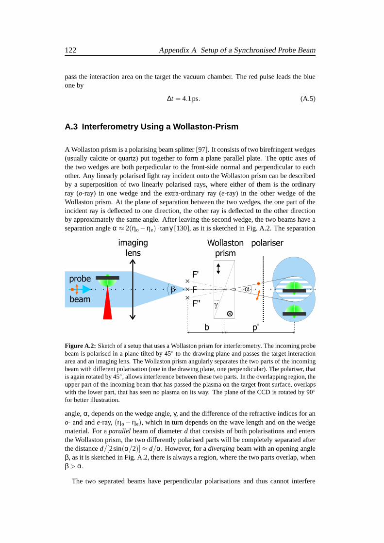
122 Appendix A Setup of a Synchronised Probe Beam
pass the interaction area on the target the vacuum chamber. The red pulse leads the blueone by
∆t = 4.1ps. (A.5)
A.3 Interferometry Using a Wollaston-Prism
A Wollaston prism is a polarising beam splitter [97]. It consists of two birefringent wedges(usually calcite or quartz) put together to form a plane parallel plate. The optic axes ofthe two wedges are both perpedicular to the front-side normal and perpendicular to eachother. Any linearly polarised light ray incident onto the Wollaston prism can be describedby a superposition of two linearly polarised rays, where either of them is the ordinaryray (o-ray) in one wedge and the extra-ordinary ray (e-ray) in the other wedge of theWollaston prism. At the plane of separation between the two wedges, the one part of theincident ray is deflected to one direction, the other ray is deflected to the other directionby approximately the same angle. After leaving the second wedge, the two beams have aseparation angleα ≈ 2(ηo−ηe) · tanγ [130], as it is sketched in Fig. A.2. The separation
F
F'
F''
imaginglens
polariserWollastonprism
probe
beam
ab ´´
´g
p'b
´
Figure A.2: Sketch of a setup that uses a Wollaston prism for interferometry. The incoming probebeam is polarised in a plane tilted by 45 to the drawing plane and passes the target interactionarea and an imaging lens. The Wollaston prism angularly separates the two parts of the incomingbeam with different polarisation (one in the drawing plane,one perpendicular). The polariser, thatis again rotated by 45, allows interference between these two parts. In the overlapping region, theupper part of the incoming beam that has passed the plasma on the target front surface, overlapswith the lower part, that has seen no plasma on its way. The plane of the CCD is rotated by 90
for better illustration.
angle,α, depends on the wedge angle,γ, and the difference of the refractive indices for ano- and ande-ray, (ηo−ηe), which in turn depends on the wave length and on the wedgematerial. For aparallel beam of diameterd that consists of both polarisations and entersthe Wollaston prism, the two differently polarised parts will be completely separated afterthe distanced/[2sin(α/2)] ≈ d/α. However, for adivergingbeam with an opening angleβ, as it is sketched in Fig. A.2, there is always a region, wherethe two parts overlap, whenβ > α.
The two separated beams have perpendicular polarisations and thus cannot interfere

A.4 Preplasma Generation Using a Synchronised Nd:Glass Laser 123
in the first place. When a polariser rotated by 45 with respect to both polarisations isinserted behind the Wollaston prism, the polariser reducesthe intensities of both beamsby a factor of 2, but they have parallel polarisations afterwards and can interfere in theoverlapping region. As the upper part of the incoming beam overlaps with the lower part,a good spatial coherence over the whole beam is required to obtain interference.1 Thedistance of the interference fringes,i, in the plane of the CCD is given by [127]
i =λL
αp′
b(A.6)
and depends on the position of the Wollaston prism between the focal spot,F, of theimaging lens and the plane of the CCD.
A setup sketched in Fig. A.2 can be used for interferometry ofa plasma, if the followingrequirements are met:
• The incoming beam has to have a good spatial coherence, what is usually satisfiedfor short-pulse lasers having inherently high spatial coherence over the beam.
• To be able to deduce the electron-density distribution fromthe interference patternin the overlapping region by Abel-inversion [131,132] whatwill be described in thenext section, the one part of the probe beam has to pass the plasma region, whilethe other part has to pass vacuum regions only that one obtains overlapping of adisturbed and a completely undisturbed beam.
Therefore the beam diameter has to be be sufficiently large tocover plasma regions aswell as undisturbed vacuum regions and the spatial separation between the two differentlypolarised beams, that depends on the image magnification andthe separation angle of theWollaston prism, has to be large enough. In the setup used here, the probe beam diameterwas 11mm and the separation of the two images of the interaction area was equivalent to∼ 1.5mm in the plane of the target, what is smaller than the preplasma extension as it wassimulated by MULTI (see below).
A.4 Preplasma Generation Using a Synchronised Nd:GlassLaser
The 2ω−probe beam described in the last two sections was used to study the preplasmaevolution driven by a synchronised frequency-doubled Nd:Glass laser that delivered pulsesof 3-ns duration and 12-J of energy at a wave length of 532nm. This external prepulse wasfocused to a spot of 200-µm diameter onto thin plastic or metal foils having an averagedintensity of 1013W/cm2. This prepulse was capable of producing a long-scale lengthpre-plasma extending over several 100’s of micrometers on the target front side. Into this pre-plasma, the synchronised CPA-laser pulse from ATLAS was focused producing a plasma
1This situation is different to a Mach-Zehnder interferometer, where after splitting and recombination of thebeam the same spatial parts overlap again.

124 Appendix A Setup of a Synchronised Probe Beam
channel that also extended over several 100’s of micrometers. First, concentrate on thepreplasma evolution and its characterisation are described, while the channel formation isdiscussed in section A.5.
Fig. A.3 (a) shows a typical interferometric image from the preplasma obtained bybacklighting the interaction region from the side with the 2ω−probe beam. Fig. A.3 (b)gives the electron-density distribution deduced from thisinterferometric picture. As theprobe-beam duration of∼ 160fs was much shorter than the time scale of the preplasmaevolution, we obtain a snap shot of the plasma at the time determined by the delay betweenNd:Glass-laser pulse and probe pulse.
(a) (b)
Figure A.3: 2ω−interferogram (a) of a preplasma produced by a Nd:Glass-laser pulse impingingon a polypropylen foil from the left and the deduced electron-density distribution (b) in units ofncr=1.79×1021cm−3. The bending of interference fringes to the left indicates an electron densityne > 0. The CPA main pulse coming from the left is not seen in the interferogram, as the probebeam was earlier by∼ 300fs. However, the bright spot in the middle of the interaction area is dueto 2ω−self emission of the plasma. The electron density distribution given in (b) corresponds tothe part of (a) indicated by the red box.
Deduction of the Electron-Density Distribution by Abel-In version
When a light ray with wave lengthλL propagates through a cylindrically symmetricelectron density,ne(r), with a minimal distance,y0 from the axis of symmetry,O, as it issketched in Fig. A.4, its phase,ϕ(y0), differs to that of a ray propagating an equivalentdistance through vacuum by
∆ϕ(y0) = Φ(y0) =2πλL
x2∫
x1
[1−η(x)]dx≈ πncrλL
x2∫
x1
ne(x)dx
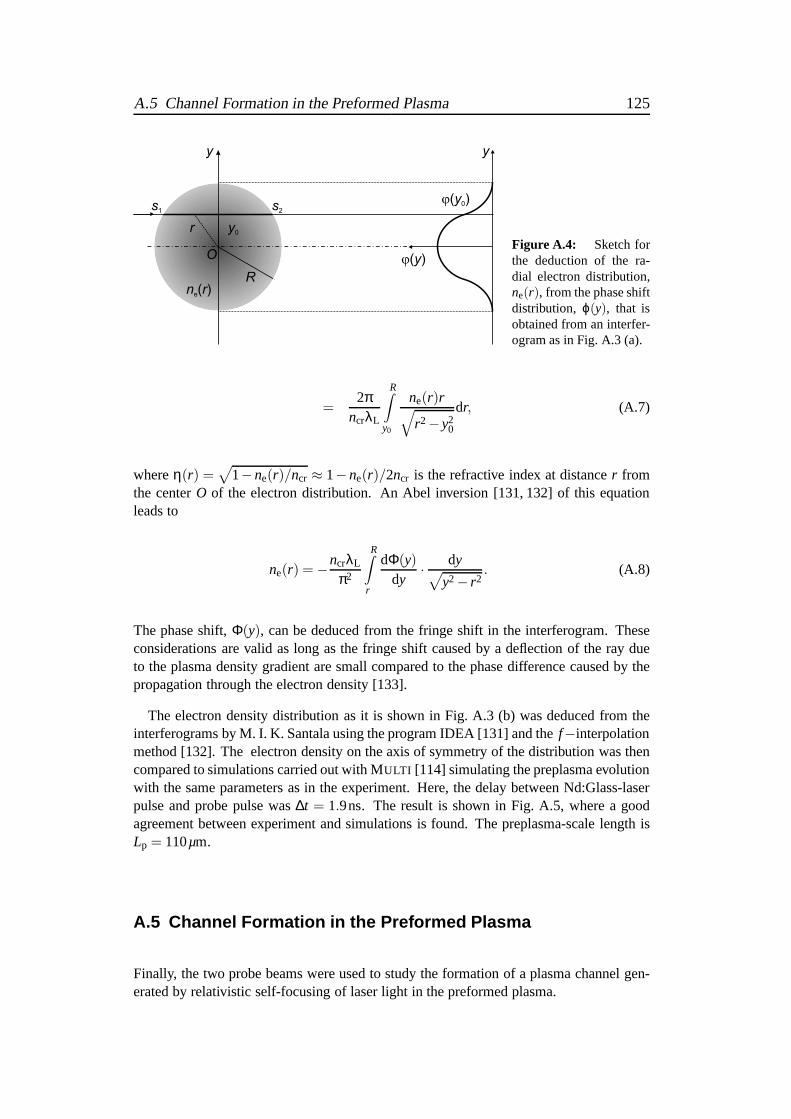
A.5 Channel Formation in the Preformed Plasma 125
j( )y0
y y
y0r
Rn re( )
j( )yO
s2s1
Figure A.4: Sketch forthe deduction of the ra-dial electron distribution,ne(r), from the phase shiftdistribution, ϕ(y), that isobtained from an interfer-ogram as in Fig. A.3 (a).
=2π
ncrλL
R∫
y0
ne(r)r√
r2−y20
dr, (A.7)
whereη(r) =√
1−ne(r)/ncr ≈ 1−ne(r)/2ncr is the refractive index at distancer fromthe centerO of the electron distribution. An Abel inversion [131, 132] of this equationleads to
ne(r) = −ncrλL
π2
R∫
r
dΦ(y)dy
· dy√
y2− r2. (A.8)
The phase shift,Φ(y), can be deduced from the fringe shift in the interferogram. Theseconsiderations are valid as long as the fringe shift caused by a deflection of the ray dueto the plasma density gradient are small compared to the phase difference caused by thepropagation through the electron density [133].
The electron density distribution as it is shown in Fig. A.3 (b) was deduced from theinterferograms by M. I. K. Santala using the program IDEA [131] and thef−interpolationmethod [132]. The electron density on the axis of symmetry ofthe distribution was thencompared to simulations carried out with MULTI [114] simulating the preplasma evolutionwith the same parameters as in the experiment. Here, the delay between Nd:Glass-laserpulse and probe pulse was∆t = 1.9ns. The result is shown in Fig. A.5, where a goodagreement between experiment and simulations is found. Thepreplasma-scale length isLp = 110µm.
A.5 Channel Formation in the Preformed Plasma
Finally, the two probe beams were used to study the formationof a plasma channel gen-erated by relativistic self-focusing of laser light in the preformed plasma.

126 Appendix A Setup of a Synchronised Probe Beam
Figure A.5: Comparisonbetween the experimen-tally measured electrondensity distribution withMULTI -simulations. For adelay between 1.2ns and2.2ns, a very good agree-ment with the experimentis found, where a delayof 1.9ns was used. In theregion measurable in theexperiment, the electrondensity can be describedby an exponential distribu-tion with a density-scalelength ofLp = 110µm.
A.5.1 Plasma Channels in Self-Emission
Fig. A.6 shows two images of the same plasma channel recordedat two different wavelengths (790nm in (a) and 395nm in (b)) without probe beams. Electrons in the plasmachannel scatter laser light sideways via linear and non-linear Thomson scattering, the in-tensity of the side-scattered light depends on the local laser intensity. The plasma channel
(a) (b)
Figure A.6: Images of a relativistic plasma channel generated by focusing the high-intensity laserpulse of ATLAS 10 into the preformed plasma. The two images of self-emittedlight are recordedat 790nm (a) and 395nm. The plasma channel extends over more than 400µm, the initial targetfront surface is indicated by the vertical dashed line.
extends over a length of more than 400µm. This is 8-times the confocal parameter ofthe vacuum focus, which is 50µm (see chapter 3). This is comparable to results obtainedin [10], where electrons were acclerated in a gas jet. Furthermore, the electron energyspectra measured with a 45-channel electron spectrometer [134] also exhibit an exponen-tial decay with a effective temperature between 2 and 5MeV. It is most likely that theelectrons are accelerated in the channel via the mechanism of direct laser acceleration(DLA), that was described in chapter 2.2.2.

A.5 Channel Formation in the Preformed Plasma 127
A.5.2 Interferometrical Pictures of Plasma Channels
In the last section the plasma channels could be observed by their self-emitted light, whichwas recorded over the whole exposure time of the CCD-camera,which is of the order ofseveral milliseconds. Therefore, the recorded images are time-integrated, as the chan-nel evolves on a sub-ps time scale. However, using the two synchronised probe beamseach having a pulse duration of∼ 150fs allows nearly time-resolved images of the rapidexpansion of the plasma channel.
Due to the ponderomotive force of the laser, electrons are radially expelled from thechannel leaving behind a region of reduced electron densityon the axis of the channel.Furthermore, a shock front, in which the local electron density encreases, propagatesradially outwards from the channel axis. Both effects, the reduction of electron densityin the center of the channel and the fast propagating shock front forming a cylindricalshell around the central axis, where the local electron density is higher, can be seen in theinterferograms. Fig. A.7 shows two interferograms of the preplasma and the channeling
(a) Interferogram with 790-nm probe beam (b) Interferogram with 395-nm probe beam
Figure A.7: Interferograms taken during the same laser shot with two differently-coloured probebeams. The 790-nm beam (a) passes the interaction area shortly before the arrival of the mainpulse in the preplasma, the 395-nm beam (b) shortly after themain pulse. Therefore, the channel-induced density modulations in the preplasma are visible in(b) but not in (a).
region of the same laser shot. While the iterferogram in (a) was generated with the 790-nmpulse, what is indicated by the red background colour, the interferogram in (b) was takenwith the blue 395-nm pulse. Depending on the intensity ratiobetween the light from thechannel self-emission and the backlighting probe beam, theself-emission is still visibleas in (a) or suppressed as in (b). In (b), only the strong emission from the laser pulseimpinging on the overcritical plasma layer is seen as an overexposed spot, while in (a) theself emission of the channel can clearly be distinguished.
However, the imprint of the channel on the electron density,i.e. a distortion of theinterference fringes that correspond to the electron density of the preplasma, can only beseen in the right picture. To estimate the delay between the two probe pulses, pictures weretaken with different delays between the main pulse and the two probe beams. Starting

128 Appendix A Setup of a Synchronised Probe Beam
from a certain delay setting, where no channel fringes couldbe observed in both pictures,the delay was increased in steps of 1.5ps, first observing the appearance of channel fringesin the 395-nm picture as shown in Fig. A.7 and then in both pictures. The upper limit forthe delay between the two probe beams was found to be 6ps whichis the total delaybetween the two delay settings, where either channel interference was observed in noneor in both of the pictures. The lower limit was 3ps. This is in good agreement with theestimation of∆t = 4.1ps from the group-velocity dispersion carried out in section A.2.These measurements show for the first time the generation of the plasma channel witha time resolution of a few ps for one single laser shot. The time delay between the twopulses estimated from the measurements agrees well with theexpected value.
Finally, the expansion of the plasma channel was measured ina series of shots with
(a) Only Nd:Glass laser, no CPA-laser (b) ∆t = −0.3ps
(c) ∆t = 0ps (d) ∆t = +0.6ps
(e) ∆t = +1.3ps (f) ∆t = +12.0ps
Figure A.8: Series of interferograms with different delays between CPA-laser pulse and2ω−probe pulse. Picture (a) was taken with the prepulse laser only.
different delays, here using only the pictures obtained with the 2ω−probe beam, as it isshown in Fig. A.8.

Bibliography
[1] D. Strickland and G. Mourou,Compression of amplified chirped optical pulses,Opt. Commun.56, 219 (1985).
[2] C. B. Edwards,Vulcan Petawatt Upgrade Overview, Central Laser Facility (CLF),Annual Report, pg. 164 (2001/2002).
[3] M. Aoyama, K. Yamakawa, Y. Akahane, J. Ma, N. Inoue, H. Ueda, andH. Kiriyama,0.85-PW, 33-fs Ti:sapphire laser, Optics Letters28, 1594 (2003).
[4] Y. Kitagawa, H. Fujita, R. Kodama, H. Yoshida, S. Matsudo, T. Jistuno,T. Kawasaki, T. Kanabe, S. Sakabe, K. Shigemori, N. Miyanaga, and Y. Izawa,Prepulse-Free Petawatt Laser for a Fast Ignition, IEEE Journal of Quantum Elec-tronics40, 281 (2004).
[5] K. Krushelnick, private communication (2004).
[6] V. Malka, S. Fritzler, E. Lefebvre, M.-M. Aleonard, F. Burgy, J.-P. Chambaret, J.-F.Chemin, K. Krushelnick, G. Malka, S. P. D. Mangles, Z. Najmudin, M. Pittman,J.-P. Rousseau, J.-N. Scheurer, B. Walton, and A. E. Dangor,Electron Accelerationby a Wake Field Forced by an Intense Ultrashort Laser Pulse, Science298, 1596(2002).
[7] E. Esarey, P. Sprangle, J. Krall, and A. Ting,Overwiew of plasma-based accelera-tor concepts, IEEE Trans. Plasma Sci.30, 252 (1996).
[8] G. Malka and J. L. Miquel,Experimental Confirmation of Ponderomotive-ForceElectrons Produced by an Ultrarelativistic Laser Pulse on aSolid Target, PhysicalReview Letters77, 75 (1996).
[9] M. H. Key, M. D. Cable, T. E. Cowan, K. G. Estabrook, B. A. Hammel, S. P.Hatchett, E. A. Henry, D. E. Hinkel, J. D. Kilkenny, J. A. Koch, W. L. Kruer, A. B.Langdon, B. F. Lasinski, R. W. Lee, B. J. MacGowan, A. MacKinnon, J. D. Moody,M. J. Moran, A. A. Offenberger, D. M. Pennington, M. D. Perry,T. J. Phillips, T. C.Sangster, M. S. Singh, M. A. Stoyer, M. Tabak, G. L. Tietbohl,M. Tsukamoto,K. Wharton, and S. C. Wilks,Hot electron production and heating by hot electronsin fast ignitor research, Physics of Plasmas5, 1966 (1998).
[10] C. Gahn, G. D. Tsakiris, A. Pukhov, J. Meyer-ter-Vehn, G. Pretzler, P. Thirolf,D. Habs, and K. J. Witte,Multi-MeV Electron Beam Generation by Direct LaserAcceleration in High-Density Plasma Channels, Physical Review Letters83, 4772(1999).
129

130 Bibliography
[11] C. Gahn, G. Pretzler, A. Saemann, G. D. Tsakiris, K. J. Witte, D. Gassmann,T. Schatz, U. Schramm, P. Thirolf, and D. Habs,MeVγ-ray yield from solid targetsirradiated with fs-laser pulses, Applied Physics Letters73, 3662 (1998).
[12] A. Maksimchuk, S. Gu, K. Flippo, D. Umstadter, and V. Yu.Bychenkov,ForwardIon Acceleration in Thin Films Driven by a High-Intensity Laser, Physical ReviewLetters84, 4108 (2000).
[13] E. L. Clark, K. Krushelnick, J. R. Davies, M. Zepf, M. Tatarakis, F. N. Beg,A. Machacek, P. A. Norreys, M. I. K. Santala, I. Watts, and A. E. Dangor,Mea-surements of Energetic Proton Transport through Magnetized Plasma from IntenseLaser Interactions with Solids, Physical Review Letters84, 670 (2000).
[14] E. L. Clark, K. Krushelnick, M. Zepf, F. N. Beg, M. Tatarakis, A. Machacek,M. I. K. Santala, I. Watts, P. A. Norreys, and A. E. Dangor,Energetic Heavy-Ionand Proton Generation from Ultraintense Laser-Plasma Interactions with Solids,Physical Review Letters85, 1654 (2000).
[15] R. A. Snavely, M. H. Key, S. P. Hatchett, T. E. Cowan, M. Roth, T. W. Phillips,M. A. Stoyer, E. A. Henry, T. C. Sangster, M. S. Singh, S. C. Wilks, A. J. Mack-innon, A. Offenberger, D. M. Penning, K. Yasuike, A. B. Langdon, B. F. Lasin-ski, J. Johnson, M. D. Perry, and E. M. Campbell,Intense High-Energy ProtonBeams from Petawatt-Laser Irradiation of Solids, Physical Review Letters85, 2945(2000).
[16] S. P. Hatchett, C. G. Brown, T. E. Cowan, E. A. Henry, J. S.Johnson, M. H. Key,J. A. Koch, A. B. Langdon, B. F. Lasinski, R. W. Lee, A. J. Mackinnon, D. M.Pennington, M. D. Perry, T. W. Phillips, M. Roth, T. C. Sangster, M. S. Singh,R. A. Snavely, M. A. Stoyer, S. C. Wilks, and K. Yasuike,Electron, photon, and ionbeams from the relativistic interaction of Petawatt laser pulses with solid targets,Physics of Plasmas7, 2076 (2000).
[17] S. C. Wilks, A. B. Langdon, T. E. Cowan, M. Roth, M. Singh,S. Hatchett, M. H.Key, D. Pennington, A. Mackinnon, and R. A. Snavely,Energetic proton genera-tion in ultra-intense laser-solid interactions, Physics of Plasmas8, 542 (2001).
[18] M. Hegelich, S. Karsch, G. Pretzler, D. Habs, K. J. Witte, W. Guenther, M. Allen,A. Blazevic, J. Fuchs, J.-C. Gauthier, M. Geissel, P. Audebert, T. E. Cowan, andM. Roth,MeV Ion Jets from Short-Pulse-Laser Interaction with Thin Foils, Physi-cal Review Letters89, 085002 (2002).
[19] G. Pretzler, A. Saemann, A. Pukhov, D. Rudolph, T. Schatz, U. Schramm, P. Thi-rolf, D. Habs, K. Eidmann, G. D. Tsakiris, J. Meyer-ter-Vehn, and K. J. Witte,Neutron production by 200 mJ ultrashort laser pulses, Physical Review E58, 1165(1998).
[20] L. Disdier, J.-P. Garconnet, G. Malka, and J.-L. Miquel, Fast neutron emissionfrom a high-energy ion beam produced by a high-intensity picosecond laser pulse,Physical Review Letters82, 1454 (1999).
Bibliography 131
[21] C. Gahn, G. D. Tsakiris, G. Pretzler, K. J. Witte, C. Delfin, C.-G. Wahlstrom, andD. Habs,Positron Generation with Table-Top Lasers, Applied Physics Letters77,2662 (2000).
[22] R. Decoste and B. H. Ripin,High-Energy Ion Expansion in Laser-Plasma Interac-tions, Physical Review Letters40, 34 (1978).
[23] C. Joshi, M. C. Richardson, and G. D. Enright,Quantitative measurements of fastions fromCO2-laser produced plasmas, Applied Physics Letters34, 625 (1979).
[24] G. D. Tsakiris, K. Eidmann, R. Petsch, and R. Sigel,Experimental Studies of theBilateral Ion Blowoff from Laser-Irradiated Thin Plastic Foils, Physical ReviewLetters46, 1202 (1981).
[25] F. Begay and D. W. Forslund,Acceleration of multi-species ions inCO2 laser-produced plasmas: Experiments and Theory, Physics of Fluids25, 1675 (1982).
[26] S. J. Gitomer, R. D. Jones, F. Begay, A. W. Ehler, J. F. Kephart, and R. Kristal,Fastions and hot electrons in the laser-plasma interaction, Physics of Fluids29, 2679(1986).
[27] M. D. Perry, D. Pennington, B. C. Stuart, G. Tietbohl, J.A. Britten, C. Brown,S. Herman, B. Golick, M. Kartz, J. Miller, H. T. Powell, M. Vergino, andV. Yanovsky,Petawatt laser pulses, Optics Letters24, 160 (1999).
[28] M. Roth, M. Allen, P. Audebert, A. Blazevic, E. Brambrink, T. E. Cowan, J. Fuchs,J. C. Gauthier, M. Geissel, M. Hegelich, S. Karsch, J. Meyer-ter-Vehn, H. Ruhl,T. Schlegel, and R. Stephens,The generation of high quality, intense ion beams byultra intense lasers, Plasma Physics and Controlled Fusion44, B99 (2002).
[29] M. Borghesi, A. J. Mackinnon, D. H. Campbell, D. G. Hicks, S. Kar, P. K. Patel,D. Price, L. Romagnani, A. Schiavi, and O. Willi,Multi-MeV Proton Source In-vestigations in Ultraintense Laser-Foil Interactions, Physical Review Letters92,055003 (2004).
[30] T. E. Cowan, J. Fuchs, H. Ruhl, A. Kemp, P. Audebert, M. Roth, R. Stephens,I. Barton, A. Blazevic, E. Brambrink, J. Cobble, J. Fernandez, J.-C. Gauthier,M. Geissel, M. Hegelich, J. Kaae, S. Karsch, G. P. Le Sage, S. Letzring, M. Man-clossi, S. Meyroneinc, A. Newkirk, H. Pepin, and N. Renard-LeGalloudec,Ul-tralow Emittance, Multi-MeV Proton Beams from a Laser Virtual-Cathode PlasmaAccelerator, Physical Review Letters92, 204801 (2004).
[31] P. K. Patel, A. J. Mackinnon, M. H. Key, T. E. Cowan, M. E. Foord, M. Allen, D. F.Price, H. Ruhl, P. T. Springer, and R. Stephens,Isochoric Heating of Solid-DensityMatter with an Ultrafast Proton Beam, Physical Review Letters91, 125004 (2003).
[32] J. A. Cobble, R. P. Johnson, T. E. Cowan, N. Renard-Le Galloudec, and M. Allen,High resolution laser-driven proton radiography, Journal of Applied Physics92,1775 (2002).

132 Bibliography
[33] M. Borghesi, S. Bulanov, D. H. Campbell, R. J. Clarke, T.Z. Esirkepov, M. Gal-imberti, L. A. Gizzi, A. J. Mackinnon, N. M. Naumova, F. Pegoraro, H. Ruhl,A. Schiavi, and O. Willi,Macroscopic Evidence of Soliton Formation in Multiter-awatt Laser-Plasma Interaction, Physical Review Letters88, 135002 (2002).
[34] A. J. Mackinnon, P. K. Patel, D. W. Price, D. Hicks, L. Romagnani, and M. Borgh-esi,Proton moire fringes for diagnosing electromagnetic fields in opaque materialsand plasmas, Applied Physics Letters82, 3188 (2003).
[35] M. Roth, T. E. Cowan, M. H. Key, S. P. Hatchett, C. Brown, W. Fountain, J. John-son, D. M. Pennington, R. A. Snavely, S. C. Wilks, K. Yasuike,H. Ruhl, F. Pego-raro, S. V. Bulanov, E. M. Campbell, M. D. Perry, and H. Powell, Fast Ignition byIntense Laser-Accelerated Proton Beams, Physical Review Letters86, 436 (2001).
[36] M. Tabak, J. Hammer, M. E. Glinsky, W. L. Kruer, S. C. Wilks, J. Woodworth,E. M. Campbell, and M. D. Perry,Ignition and high gain with ultrapowerful lasers,Physics of Plasmas1, 1626 (1994).
[37] M. Roth, T. E. Cowan, J. C. Gauthier, M. Allen, P. Audebert, A. Blazevic, J. Fuchs,M. Geissel, M. Hegelich, S. Karsch, J. Meyer-ter-Vehn, A. Pukhov, and T. Schlegel,Energetic ions generated by laser pulses: A detailed study on target properties,Physical Review Special Topics - Accelerators and Beams5, 061301 (2002).
[38] A. J. Mackinnon, Y. Sentoku, P. K. Patel, D. W. Price, S. Hatchett, M. H. Key,C. Andersen, R. Snavely, and R. R. Freeman,Enhancement of Proton Accelera-tion by Hot-Electron Recirculation in Thin Foils Irradiated by Ultraintense LaserPulses, Physical Review Letters88, 215006 (2002).
[39] I. Spencer, K. W. D. Ledingham, P. McKenna, T. McCanny, P. Singhal, S. Foster,D. Neely, A. J. Langley, E. J. Divall, C. J. Hooker, R. J. Clarke, P. A. Norreys, E. L.Clark, K. Krushelnick, and J. R. Davies,Experimental study of proton emissionfrom 60-fs, 200-mJ high-repetition-rate tabletop-laser pulses interacting with solidtargets, Physical Review E67, 046402 (2003).
[40] L. Pommier and E. Lefebvre,Simulations of energetic proton emission in laser-plasma interaction, Laser and Particle Beams21, 573 (2003).
[41] M. Passoni, V. T. Tikhonchuk, M. Lontano, and V. Yu. Bychenkov,Charge sepa-ration effects in solid targets and ion acceleration with a two-temperature electrondistribution, Physical Review E69, 026411 (2004).
[42] A. J. Mackinnon, M. Borghesi, S. Hatchett, M. H. Key, P. K. Patel, H. Campbell,A. Schiavi, R. Snavely, S. C. Wilks, and O. Willi,Effect of Plasma Scale Lengthon Multi-MeV Proton Production by Intense Laser Pulses, Physical Review Letters86, 1769 (2001).
[43] S. Karsch, S. Dusterer, H. Schwoerer, F. Ewald, D. Habs, M. Hegelich, G. Pretzler,A. Pukhov, K. J. Witte, and R. Sauerbrey,High-Intensity Laser Induced Ion Accel-eration from Heavy-Water Droplets, Physical Review Letters91, 015001 (2003).
Bibliography 133
[44] M. Zepf, E. L. Clark, F. N. Beg, R. J. Clarke, A. E. Dangor,A. Gopal, K. Krushel-nick, P. A. Norreys, M. Tatarakis, U. Wagner, and M. S. Wei,Proton Accelerationfrom High-Intensity Laser Interactions with Thin Foil Targets, Physical ReviewLetters90, 064801 (2003).
[45] A. Pukhov,Three-Dimensional Simulations of Ion Acceleration from a Foil Irradi-ated by a Short-Pulse Laser, Physical Review Letters86, 3562 (2001).
[46] Y. Murakami, Y. Kitagawa, Y. Sentoku, M. Mori, R. Kodama, K. A. Tanaka,K. Mima, and T. Yamanaka,Observation of proton rear emission and possible gi-gagauss scale magnetic fields from ultra-intense laser illuminated plastic targets,Physics of Plasmas8, 4138 (2001).
[47] M. Kaluza, J. Schreiber, M. I. K. Santala, G. D. Tsakiris, K. Eidmann, J. Meyer-ter-Vehn, and K. J. Witte,Influence of the Laser Prepulse on Proton Accelerationin Thin-Foil Experiments, Physical Review Letters93, 045003 (2004).
[48] J. J. Honrubia, M. Kaluza, G. D. Tsakiris, and J. Meyer-ter-Vehn,Fast electronpropagation in non-uniform plasmas, to be submitted to Physical Review E (2004).
[49] H. Baumhacker, G. Pretzler, K. J. Witte, M. Hegelich, M.Kaluza, S. Karsch,A. Kudryashov, V. Samarkin, and A. Roukossouev,Correction of strong phase andamplitude modulations by two deformable mirrors in a multistaged Ti:sapphirelaser, Optics Letters27, 1570 (2002).
[50] K. Eidmann, J. Meyer-ter-Vehn, T. Schlegel, and S. Huller, Hydrodynamic simu-lation of subpicosecond laser interaction with solid-density matter, Physical Re-view E62, 1202 (2000).
[51] E. S. Sarachik and G. T. Schappert,Classical Theory of the Scattering of IntenseLaser Radiation by Free Electrons, Physical Review A1, 2738 (1970).
[52] L. D. Landau and E. M. Lifschitz,Lehrbuch der theoretischen Physik: KlassischeFeldtheorie, S. 132, Akademie-Verlag, Berlin, 7. Ed. (1977).
[53] P. Gibbon,High-Order Harmonic Generation in Plasmas, IEEE Journal of Quan-tum Electronics33, 1915 (1997).
[54] C. I. Moore, J. P. Knauer, and D. D. Meyerhofer,Observation of the Transition fromThomson to Compton Scattering in Multiphoton Interactionswith Low-EnergyElectrons, Physical Review Letters74, 2439 (1995).
[55] F. V. Hartemann, S. N. Fochs, G. P. Le Sage, N. C. Luhrmann, Jr., J. G. Woodworth,M. D. Perry, Y. J. Chen, and A. K. Kerman,Nonlinear ponderomotive scattering ofrelativistic electrons by an intense laser field at focus, Physical Review E51, 4833(1995).
[56] F. V. Hartemann, J. R. Van Meter, A. L. Troha, E. C. Landahl, N. C. Luhmann, Jr.,H. A. Baldis, A. Gupta, and A. K. Kerman,Three-dimensional relativistic electronscattering in an ultrahigh-intensity laser focus, Physical Review E58, 5001 (1998).
134 Bibliography
[57] G. Malka, E. Lefebvre, and J. L. Miquel,Experimental Observation of ElectronsAccelerated in Vacuum to Relativistic Energies by a High-Intensity Laser, PhysicalReview Letters78, 3341 (1997).
[58] F. F. Chen,Introduction to Plasma Physics, Plenum Press, New York (1974).
[59] W. L. Kruer, The Physics of Laser Plasma Interactions, Addison-Wesley, NewYork (1988).
[60] B. Quesnel and P. Mora,Theory and simulation of the interaction of ultraintenselaser pulses with electrons in vacuum, Physical Review E58, 3719 (1998).
[61] J. Meyer-ter-Vehn, A. Pukhov, and Z. M. Sheng,Relativistic Laser Plasma In-teraction, in: Atoms, Solids, and Plasmas in Super-Intense Laser Fields (edi-tors: D. Batani, C. J. Joachain, S. Martellucci, and A. N. Chester), Kluwer Aca-demic/Plenum Publishers, New York (2001).
[62] E. Lefebvre and G. Bonnaud,Transparency/Opacity of a Solid Target Illuminatedby an Ultrahigh-Intensity Laser Pulse, Physical Review Letters74, 2002 (1995).
[63] G.-Z. Sun, E. Ott, Y. C. Lee, and P. Guzdar,Self-focusing of short intense pulses inplasmas, Physics of Fluids30, 526 (1987).
[64] H. Alfven, On the motion of cosmic rays in interstellar space, Physical Review55,429 (1939).
[65] A. Pukhov and J. Meyer-ter-Vehn,Laser Hole Boring into Overdense Plasma andRelativistic Electron Currents for Fast Ignition of ICF Targets, Physical ReviewLetters79, 2686 (1997).
[66] H. Ruhl, Y. Sentoku, K. Mima, K. A. Tanaka, and R. Kodama,Collimated ElectronJets by Intense Laser-Beam-Plasma Surface Interaction under Oblique Incidence,Physical Review Letters82, 743 (1999).
[67] S. C. Wilks, D. L. Kruer, M. Tabak, and A. B. Langdon,Absorption of Ultra-Intense Laser Pulses, Physical Review Letters69, 1383 (1992).
[68] F. Brunel,Not-so-Resonant, Resonant Absorption, Physical Review Letters59, 52(1987).
[69] T. Tajima and J. M. Dawson,Laser Electron Accelerator, Physical Review Letters43, 267 (1979).
[70] A. Pukhov and J. Meyer-ter-Vehn,Relativistic laser-plasma interaction by multi-dimensional particle-in-cell simulations, Physics of Plasmas5, 1880 (1998).
[71] A. Pukhov, Z.-M. Sheng, and J. Meyer-ter-Vehn,Particle acceleration in relativis-tic laser channels, Physics of Plasmas6, 2847 (1999).
[72] M. Borghesi, A. J. MacKinnon, L. Barringer, R. Gaillard, L. A. Gizzi, C. Meyer,O. Willi, A. Pukhov, and J. Meyer-ter-Vehn,Relativistic Channeling of a Picosec-ond Laser Pulse in a Near-Critical Preformed Plasma, Physical Review Letters78,879 (1997).

Bibliography 135
[73] M. I. K. Santala, M. Zepf, I. Watts, F. N. Beg, E. Clark, M.Tatarakis, K. Krushel-nick, A. E. Dangor, T. McCanny, I. Spencer, R. P. Singhal, K. W. D. Ledingham,S. C. Wilks, A. C. Machacek, J. S. Wark, R. Allott, R. J. Clarke, and P. A. Norreys,Effect of the Plasma Density Scale Length on the Direction ofFast Electrons inRelativistic Laser-Solid Interactions, Physical Review Letters84, 1459 (2000).
[74] F. Brandl, G. Pretzler, D. Habs, and E. Fill,Cerenkov radiation diagnostics of hotelectrons generated by fs-laser interaction with solid targets, Europhysics Letters61, 632 (2002).
[75] V. T. Tikhonchuk,Interaction of a beam of fast electrons with solids, Physics ofPlasmas9, 1416 (2002).
[76] E. S. Weibel,Spontaneously growing transverse waves in a plasma due to ananisotropic velocity distribution, Physical Review Letters2, 83 (1959).
[77] M. Honda, J. Meyer-ter-Vehn, and A. Pukhov,Collective Stopping and Ion Heatingin Relativistic-Electron-Beam Transport for Fast Ignition, Physical Review Letters85, 2128 (2000).
[78] H. M. Milchberg, R. R. Freeman, and S. C. Davey,Resistivity of a Simple Metalfrom Room Temperature to106 K, Physical Review Letters61, 2364 (1988).
[79] A. R. Bell and R. J. Kingham,Resistive Collimation of Electron Beams in Laser-Produced Plasmas, Physical Review Letters91, 035003 (2003).
[80] J. J. Honrubia, A. Antonicci, and D. Moreno,Hybrid simulations of fast electronstransport in conducting media, Laser and Particle Beams22, 137 (2004).
[81] Y. Sentoku, T. E. Cowan, A. Kemp, and H. Ruhl,High energy proton accelerationin interaction of short laser pulse with dense plasma target, Physics of Plasmas10,2009 (2003).
[82] B. M. Hegelich,Acceleration of heavy Ions to MeV/nucleon Energies by Ultrahigh-Intensity Lasers, Dissertation, Ludwig-Maximilians Universitat, Munchen (2002).
[83] M. Widner, I. Alexeef, and W. D. Jones,Plasma Expansion into a Vacuum, Physicsof Fluids14, 795 (1971).
[84] J. E. Crow, P. L. Auer, and J. E. Allen,The expansion of a plasma into a vacuum,Journal of Plasma Physics14, 65 (1975).
[85] J. Denavit,Collisionless plasma expansion into a vacuum, Physics of Fluids22,1384 (1979).
[86] P. Mora,Plasma Expansion into a Vacuum, Physical Review Letters90, 185002(2003).
[87] M. Kaluza,Ionisation von Hoch-Z-Atomen in starken Laserfeldern, Diplomarbeit,Technische Universitat, Munchen (2000).
[88] A. V. Gurevich, L. V. Pariiskaya, and L. P. Pitaevskii,Self-Similar Motion of Rar-efied Plasma, Soviet Physics JETP22, 449 (1966).
136 Bibliography
[89] P. Mora, private communication (2004).
[90] H. Baumhacker, A. Boswald, H. Haas, M. Fischer, W. Folsner, G. Keller, U. Andiel,X. Dong, M. Dreher, K. Eidmann, E. Fill, M. Hegelich, M. Kaluza, S. Karsch,G. Pretzler, G. D. Tsakiris, and K. J. Witte,Advanced Titanium:Sapphire LaserATLAS, MPQ-Report272(2002).
[91] T. Juji, A. Unterhuber, V. S. Yakovlev, G. Tempea, A. Stingl, F. Krausz, andW. Drexler,Generation of smooth, ultra-broadband spectra directly from a prism-less Ti:sapphire laser, Applied Physics B77, 125 (2003).
[92] M. Nisoli, S. Stagira, S. De Silvestri, O. Svelto, S. Sartania, Z. Cheng, M. Lenzner,C. Spielmann, and F. Krausz,A novel high-energy pulse compression system: gen-eration of multigigawatt sub-5-fs pulses, Applied Physics B65, 189 (1997).
[93] M. D. Perry and G. Mourou,Terawatt to Petawatt Subpicosecond Lasers, Science264, 917 (1994).
[94] M. Pittman, S. Ferre, J. P. Rousseau, L. Notebaert, J. P. Chambaret, andG. Cheriaux,Design and characterization of a near-diffraction-limited femtosec-ond 100-TW 10-Hz high-intensity laser system, Applied Physics B74, 529 (2003).
[95] M. P. Kalachnikov, V. Karpov, and H. Schonnagel,100-terawatt titanium-sapphirelaser system, Laser Phys.02, 368 (2002).
[96] T. Brabec, C. Spielmann, P. F. Curley, and F. Krausz,Kerr lens mode locking,Optics Letters17, 1292 (1992).
[97] E. Hecht,Optics, Addison-Wesley, New York, 3. Ed. (1998).
[98] R. Tommasini, private communication (2004).
[99] Kentech Instruments Ltd., Harrow, U.K., http://www.kentech.co.uk.
[100] R. P. Godwin, C. G. M. van Kessel, J. N. Olsen, P. Sachsenmaier, R. Sigel,and K. Eidmann,Reflection Losses from Laser-Produced Plasmas, Zeitschrift furNaturforschung32a, 1100 (1977).
[101] Centronic Ltd., New Abingdon, Surrey, U.K., http://www.kentech.co.uk.
[102] Tektronix Inc., Beaverton, Oregon, U.S.A., http://www.tek.com.
[103] Laser 2000 GmbH, Wessling, Germany, http://www.laser2000.de.
[104] Track Analysis Systems Limited, H. H. Wills Physics Laboratory, Bristol, UK,http://www.phy.bris.ac.uk/research/TASL/home.html.
[105] S. A. Durrani and R. K. Bull,Solid State Nuclear Track Detection, Pergamon Press,Oxford (1987).
[106] National Institute of Standards and Technology, http://physics.nist.gov.
[107] J. S. Pearlman,Faraday cups for laser plasmas, Review of Scientific Instruments48, 1048 (1977).
Bibliography 137
[108] B. H. Ripin and R. Decoste,Secondary Electron Supression in Charge Collectorsand Analyzers, Naval Research Laboratory, Memorandum Report 3494, Washing-ton, D.C. (1977).
[109] S. Karsch,High-intensity laser generated neutrons: A novel neutron source andnew tool for plasma diagnostics, Dissertation, Ludwig-Maximilians Universitat,Munchen (2002).
[110] J. Schreiber, private communication (2004).
[111] Computer Simulation Technology (CST), EM STUDIOTM.
[112] Goodfellow GmbH, Bad Nauheim, Germany, http://www.goodfellow.com.
[113] D. A. Lide,CRC Handbook of Chemistry and Physics 1973-1974, CRC Press, BocaRaton, 54. Ed. (1973).
[114] R. Ramis, R. Schmalz, and J. Meyer-ter-Vehn,MULTI: A computer code for one-dimensional multigroup radiation hydrodynamics, Computer Physics Communica-tions88, 475 (1988).
[115] Y. B. Zel’dovich and Y. P. Raizer,Physics of Shock Waves and High-TemperatureHydrodynamic Phenomena, Academic Press, New York (1966).
[116] T4 Group, SESAME Equation Of State, Los Alamos National Laboratory, Re-port LALP-83-4, Los Alamos, NM (1983).
[117] K. Eidmann,Radiation transport and atomic physics modeling in high-energy-density alser-produced plasmas, Laser and Particle Beams12, 223 (1994).
[118] J. Stein, private communication (2004).
[119] W. Press, B. Flannery, S. Teukolsky, and W. Vetterling, Numerical Recipes in C:The Art of Scientific Computing, Cambridge University Press, New York, 2. Ed.(1992).
[120] L. M. Wickens, J. E. Allen, and P. T. Rumsby,Ion emission from Laser-ProducedPlasmas with Two Electron Temperatures, Physical Review Letters41, 243 (1978).
[121] J. Davies, A. R. Bell, and M. Tatarakis,Magnetic focusing and trapping of high-intensity laser-generated fast electrons at the rear of solid targets, Physical Re-view E59, 6032 (1999).
[122] Y. T. Lee and R. M. More,An electron conductivity model for dense plasmas,Physics of Fluids5, 1273 (1984).
[123] A. Pukhov, Three-dimensional electromagnetic relativistic particle-in-cell codeVLPL (Virtual Laser Plasma Lab), Journal of Plasma Physics61, 425 (1999).
[124] H. Ruhl, private communication (unpublished) (2003).
[125] M. Roth, private communication (2004).
[126] J. J. Honrubia, private communication (2004).
138 Bibliography
[127] R. Benattar, C. Popovics, and R. Sigel,Polarized light interferometer for laserfusion studies, Review of Scientific Instruments50, 1583 (1979).
[128] A. Pukhov and J. Meyer-ter-Vehn,Relativistic Magnetic Self-Channeling of Lightin Near-Critical Plasma: Three-Dimensional Particle-in-Cell Simulation, PhysicalReview Letters76, 3975 (1996).
[129] Schott Glaskatalog, http://www.schott.de.
[130] M. Francon and S. Mallick,Polarization Interferometers, Wiley-Interscience, Lon-don, 1. Ed. (1971).
[131] M. Hipp and P. Reiterer,User Manual for IDEA 1.00: Software for Interferomet-rical Data Evaluation, http://optics.tu-graz.ac.at, Institut fur Experimentalphysik,Technische Universitat Graz (1999).
[132] G. Pretzler, H. Jager, T. Neger, H. Phillip, and J. Woisetschlager,Comparison ofDifferent Methods of Abel Inversion Using Computer Simulated and ExperimentalSide-On Data, Zeitschrift fur Naturforschung47a, 955 (1992).
[133] K.-U. Amthor, Plasmadiagnose in Experimenten zur Wechselwirkung intensiverLaserimpulse mit Materie, Diplomarbeit, Friedrich-Schiller Universitat, Jena(2002).
[134] C. Gahn, G. D. Tsakiris, K. J. Witte, P. Thirolf, and D. Habs,A novel 45-channelelectron spectrometer for high intensity laser-plasma interaction studies, Reviewof Scientific Instruments71, 1642 (2000).

Appendix P
Publication List
1. M. Kaluza, J. Schreiber, M. I. K. Santala, G. D. Tsakiris, K. Eidmann, J. Meyer-ter-Vehn, and K. J. Witte:Influence of the Laser Prepulse on Proton Accelerationin Thin-Foil Experiments, Physical Review Letters,93, 045003 (2004)
2. H. Baumhacker, G. Pretzler, K.-J. Witte, M. Hegelich,M. Kaluza, S. Karsch,A. Kudryashov, V. Samarkin, and A. Roukossouev:Correction of strong phaseand amplitude modulations by two deformable mirrors in a multistaged Ti:sapphirelaser, Optics Letters,27, 1570-1572 (2002)
3. J. J. Honrubia,M. Kaluza, G. D. Tsakiris, and J. Meyer-ter-Vehn:Fast-electronpropagation in non-uniform plasmas, to be submitted to Physical Review E
The first two publications are attached to this work.
139
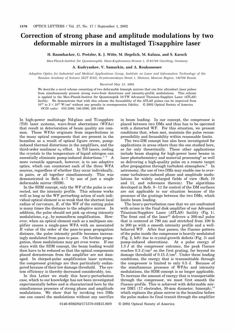
1570 OPTICS LETTERS / Vol. 27, No. 17 / September 1, 2002
Correction of strong phase and amplitude modulations by twodeformable mirrors in a multistaged Ti:sapphire laser
H. Baumhacker, G. Pretzler, K. J. Witte, M. Hegelich, M. Kaluza, and S. Karsch
Max-Planck-Institut für Quantenoptik, Hans-Kopfermann-Strasse 1, D-85748 Garching, Germany
A. Kudryashov, V. Samarkin, and A. Roukossouev
Adaptive Optics for Industrial and Medical Applications Group, Institute on Laser and Information Technology of the
Russian Academy of Science (ILIT RAS), Svyatoozerskaya Street 1, Shatura, Moscow Region, 140700 Russia
Received May 23, 2002
We describe a novel scheme consisting of two deformable bimorph mirrors that can free ultrashort laser pulsesfrom simultaneously present strong wave-front distortions and intensity-profile modulations. This schemeis applied to the Max-Planck-Institut für Quantenoptik 10-TW Advanced Titanium-Sapphire Laser (ATLAS)facility. We demonstrate that with this scheme the focusability of the ATLAS pulses can be improved from1018 to 2 3 1019 Wcm2 without any penalty in recompression fidelity. © 2002 Optical Society of America
OCIS codes: 010.1080, 140.3590, 220.1000.
In high-power multistage Nd:glass and Ti:sapphire(TiS) laser systems, wave-front aberrations (WFAs)that result in deterioration of beam quality are com-mon. These WFAs originate from imperfections inthe many optical components that are present in thebeamline as a result of optical f igure errors, pump-induced thermal distortions in the amplif iers, and thethird-order nonlinear n2 effect. In TiS lasers, coolingthe crystals to the temperature of liquid nitrogen canessentially eliminate pump-induced distortions.1 – 3 Amore versatile approach, however, is to use adaptiveoptics, which can counteract each of the three WFAsources, regardless of whether they occur individually,in pairs, or all together simultaneously. This wasdemonstrated in Refs. 4–7 by use of just a singledeformable mirror (SDM).
In the SDM concept, only the WF of the pulse is cor-rected, not the intensity profile. This scheme workswell as long as the WF perturbing action of each indi-vidual optical element is so weak that the shortest localradius of curvature, R, of the WF of the exiting pulseis many times the distance to the adaptive mirror. Inaddition, the pulse should not pick up strong intensitymodulations, e.g., by nonuniform amplification. How-ever, when an optical element such as a multipass am-plifier causes a single-pass WFA with an associatedR value of the order of the pass-to-pass propagationdistance, the pulse intensity profile becomes increas-ingly modulated from pass to pass. On further propa-gation, these modulations may get even worse. If onestays with the SDM concept, the beam loading wouldthen have to be reduced so that the optical componentsplaced downstream from the amplif ier are not dam-aged. In chirped-pulse amplification laser systems,the compressor gratings are then particularly endan-gered because of their low damage threshold. The sys-tem efficiency is thereby decreased considerably, too.
In this Letter we study this heavy-perturbationcase, which to our knowledge has not been investigatedexperimentally before and is characterized here by thesimultaneous presence of strong phase and amplitudemodulations. We show that by invoking two DMsone can cancel the modulations without any sacrif ice
in beam loading. In our concept, the compressor isplaced between two DMs and thus has to be operatedwith a distorted WF. For this situation, we presentconditions that, when met, maintain the pulse recom-pressibility and focusability within reasonable limits.
The two-DM concept has also been investigated forapplications in areas others than the one studied here,so far only theoretically. These other applicationsinclude beam shaping for high-power laser beams inlaser photochemistry and material processing8 as wellas delivering a high-quality pulse on a remote targetafter propagation through turbulent atmosphere.9 Inastronomy, the use of two DMs may enable one to over-come turbulence-induced phase and amplitude modu-lations for widely enlarged fields of view (Refs. 10and 11, and references therein). The algorithmsdeveloped in Refs. 8–11 for control of the DM surfacesare not applicable to our situation because of thepresence of the gratings between the two DMs, whichlimits beam loading.
The heavy-perturbation case that we are confrontedwith arises in the f inal disk amplif ier of our AdvancedTitanium:Sapphire Laser (ATLAS) facility (Fig. 1).The front end of the laser12 delivers a 300-mJ pulsethat is centered at 790 nm and stretched from 100 fsto 200 ps with a smooth intensity profile and a well-behaved WF. After four passes, the f luence patternof the pulse inside the compressor is heavily modulated(Fig. 2, left) due to crystal-growth defects (Fig. 3) andpump-induced aberrations. At a pulse energy of1.3 J at the compressor entrance, the peak f luencereaches 0.3 Jcm2 on the f irst grating, far beyond itsdamage threshold of 0.15 Jcm2. Under these loadingconditions, the energy that is transmittable throughthe compressor is limited to only 0.5 J. Because ofthe simultaneous presence of WFAs and intensitymodulations, the SDM concept is no longer applicable.To increase the amount of energy that is transportablethrough the compressor, we must f irst smooth thef luence profile. This is achieved with deformable mir-ror DM1 (17 electrodes, 30-mm diameter, bimorph),13
which replaces the plane mirror in the beamline beforethe pulse makes its final transit through the amplif ier
0146-9592/02/171570-03$15.00/0 © 2002 Optical Society of America

September 1, 2002 / Vol. 27, No. 17 / OPTICS LETTERS 1571
Fig. 1. Setup of the final amplif ier in the ATLAS facilitywith two deformable mirrors, DM1 and DM2, closed loop,and three target chambers (TCH5–TCH7). The TiS crys-tal of 40-mm outer diameter is pumped from two sides.The TiS pulse provided by the front end passes throughthe crystal four times and is thereby amplif ied from 0.3 to1.5 J. The pulse then runs through spatial filter SF2, andthe pulse diameter increases from 18 to 63 mm. The pulseis then recompressed to 130 fs in an evacuated compressorchamber that houses two holographic gold gratings and isconnected to the target chambers by evacuated tubes.
(Fig. 1). The best electrode voltage settings for DM1can be found manually with a few iterations by use ofa real-time beam-profile analyzer. For the sameenergy of 1.3 J as before, the peak f luence of thesmoothed profile is then reduced to 90 mJcm2 so thatthe 1.3-J energy can be safely transmitted throughthe compressor. At constant voltage settings, thesmoothed beam profile remains stable over weeks andchanges little on propagation inside the compressorand a few meters downstream.
The action of DM1 modif ies the WFAs originatingin the amplifying crystal but does not generate aplane WF. A plane WF is generated with a sec-ond deformable mirror, DM2 (33 electrodes, 80-mmdiameter, bimorph).13 DM2 is placed behind thecompressor so that it is able to compensate for theoptical f igure errors of the gratings and to ensure thathighly peaked intensity patterns that might occurwhen DM2 is optimized cannot damage the gratings.The compressor is thus fed with a chirped pulse whoseWF is distorted. In this situation, which was inves-tigated theoretically in Ref. 14, the following threeeffects are of major importance: loss of compressionfidelity, astigmatism, and chromatic aberration. Foran estimate of the level of WFAs that are tolerablewithout too high a loss in beam quality, the rigoroustheory14 is not needed. It is sufficient to replace thereal pulse with a spherical WF whose curvature ischosen to be equal to the maximum local curvature inthe real distorted WF. The focus of the model WF isdownstream DM2.
From measurements, we find that the recompres-sion fidelity in terms of pulse duration and contrastis hardly affected as long as any local radius of curva-ture of the WF exceeds 15 m. The condition is metin the ATLAS for pulse energies of up to 1 J aftercompression.
The originally spherically convergent beam turnsastigmatic when it leaves the compressor, leading tothe occurrence of two focal lines instead of a singlepoint focus because the beam behaves differentlyin the dispersion and nondispersion planes of thecompressor. With R $ m, the compressor-inducedastigmatism turns out to be weak and is hence easilycorrectable with DM2, since the necessary displace-ment is #1 mm. The compensation of the originalbeam convergence is not a problem, either.
The chromatic aberration originates from the differ-ent path lengths of the individual spectral componentson their way through the compressor. When they areexiting, the individual spectral beam components stillhave the same cone angle, but at a f ixed position inspace the radii of curvature are different. This ef-fect cannot be compensated for with DM2. The beamemerging from DM2 will hence be parallel for the spec-tral component near l0 but divergent for the compo-nents with l , l0 and convergent for those with l . l0.The focus of such a beam is hence no longer pointlikebut exhibits longitudinal spreading, with each spec-tral component having its own focus located at a dif-ferent position. This spreading is tolerable when thefoci of all colors inside the spectral range 4DlFWHM
lie within the Rayleigh length of the spectral beamcomponent at l0. For the ATLAS, this criterion re-quires R . 15 m, which is met. The theoretical analy-sis reveals that R ~ DlFWHM. Very short pulses withDlWFHM $ 50 nm thus need to be rather well collimatedif one wishes to avoid intensity degradation in the fo-cus. This conclusion is in fair agreement with the re-sults of the rigorous theory.14
Fig. 2. Fluence patterns in the plane of the first compres-sor grating. Left, DM1 is replaced with a plane mirror;peak f luence, 300 mJcm2. The double-peak pattern isdue to the coarse two-half structure of the WFAs shownin Fig. 3. Right, DM1 is optimized; peak f luence reducedto 90 mJcm2. The remaining f luence modulation arisesfrom the fine structure of the WFAs (Fig. 3). The veryhigh spatial frequencies, which carry little energy, are loston propagation through the spatial filter SF2 (Fig. 1).
Fig. 3. WFAs that are due to growth defects in the f inaldisk amplifier of 40-mm diameter, 17-mm thickness, andal 2.3 at 532 nm.
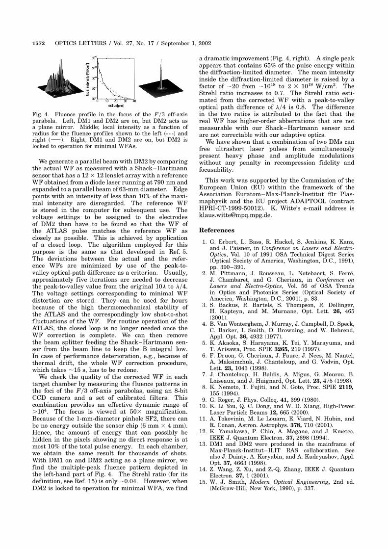
1572 OPTICS LETTERS / Vol. 27, No. 17 / September 1, 2002
Fig. 4. Fluence profile in the focus of the F3 off-axisparabola. Left, DM1 and DM2 are on, but DM2 acts asa plane mirror. Middle; local intensity as a function ofradius for the f luence profiles shown to the left - - - andright 222. Right, DM1 and DM2 are on, but DM2 islocked to operation for minimal WFAs.
We generate a parallel beam with DM2 by comparingthe actual WF as measured with a Shack–Hartmannsensor that has a 12 3 12 lenslet array with a referenceWF obtained from a diode laser running at 790 nm andexpanded to a parallel beam of 63-mm diameter. Edgepoints with an intensity of less than 10% of the maxi-mal intensity are disregarded. The reference WFis stored in the computer for subsequent use. Thevoltage settings to be assigned to the electrodesof DM2 then have to be found so that the WF ofthe ATLAS pulse matches the reference WF asclosely as possible. This is achieved by applicationof a closed loop. The algorithm employed for thispurpose is the same as that developed in Ref. 5.The deviations between the actual and the refer-ence WFs are minimized by use of the peak-to-valley optical-path difference as a criterion. Usually,approximately f ive iterations are needed to decreasethe peak-to-valley value from the original 10l to l4.The voltage settings corresponding to minimal WFdistortion are stored. They can be used for hoursbecause of the high thermomechanical stability ofthe ATLAS and the correspondingly low shot-to-shotf luctuations of the WF. For routine operation of theATLAS, the closed loop is no longer needed once theWF correction is complete. We can then removethe beam splitter feeding the Shack–Hartmann sen-sor from the beam line to keep the B integral low.In case of performance deterioration, e.g., because ofthermal drift, the whole WF correction procedure,which takes 15 s, has to be redone.
We check the quality of the corrected WF in eachtarget chamber by measuring the f luence patterns inthe foci of the F3 off-axis parabolas, using an 8-bitCCD camera and a set of calibrated filters. Thiscombination provides an effective dynamic range of.104. The focus is viewed at 503 magnification.Because of the 1-mm-diameter pinhole SF2, there canbe no energy outside the sensor chip 6 mm 3 4 mm.Hence, the amount of energy that can possibly behidden in the pixels showing no direct response is atmost 10% of the total pulse energy. In each chamber,we obtain the same result for thousands of shots.With DM1 on and DM2 acting as a plane mirror, wefind the multiple-peak f luence pattern depicted inthe left-hand part of Fig. 4. The Strehl ratio (for itsdefinition, see Ref. 15) is only 0.04. However, whenDM2 is locked to operation for minimal WFA, we find
a dramatic improvement (Fig. 4, right). A single peakappears that contains 65% of the pulse energy withinthe diffraction-limited diameter. The mean intensityinside the diffraction-limited diameter is raised by afactor of 20 from 10
18 to 2 3 1019 Wcm2. The
Strehl ratio increases to 0.7. The Strehl ratio esti-mated from the corrected WF with a peak-to-valleyoptical path difference of l4 is 0.8. The differencein the two ratios is attributed to the fact that thereal WF has higher-order abberrations that are notmeasurable with our Shack–Hartmann sensor andare not correctable with our adaptive optics.
We have shown that a combination of two DMs canfree ultrashort laser pulses from simultaneouslypresent heavy phase and amplitude modulationswithout any penalty in recompression fidelity andfocusability.
This work was supported by the Commission of theEuropean Union (EU) within the framework of theAssociation Euratom–Max-Planck-Institut für Plas-maphysik and the EU project ADAPTOOL (contractHPRI-CT-1999-50012). K. Witte’s e-mail address [email protected].
References
1. G. Erbert, L. Bass, R. Hackel, S. Jenkins, K. Kanz,and J. Paisner, in Conference on Lasers and Electro-Optics, Vol. 10 of 1991 OSA Technical Digest Series(Optical Society of America, Washington, D.C., 1991),pp. 390–391.
2. M. Pittmann, J. Rousseau, L. Notebaert, S. Ferré,J. Chambaret, and G. Cheriaux, in Conference onLasers and Electro-Optics, Vol. 56 of OSA Trendsin Optics and Photonics Series (Optical Society ofAmerica, Washington, D.C., 2001), p. 83.
3. S. Backus, R. Bartels, S. Thompson, R. Dollinger,H. Kapteyn, and M. Murnane, Opt. Lett. 26, 465(2001).
4. B. Van Wonterghem, J. Murray, J. Campbell, D. Speck,C. Barker, I. Smith, D. Browning, and W. Behrend,Appl. Opt. 36, 4932 (1977).
5. K. Akaoka, S. Harayama, K. Tei, Y. Marayuma, andT. Arisawa, Proc. SPIE 3265, 219 (1997).
6. F. Druon, G. Cheriaux, J. Faure, J. Nees, M. Nantel,A. Maksimchuk, J. Chanteloup, and G. Vodvin, Opt.Lett. 23, 1043 (1998).
7. J. Chanteloup, H. Baldis, A. Migus, G. Mourou, B.Loiseaux, and J. Huignard, Opt. Lett. 23, 475 (1998).
8. K. Nemoto, T. Fujiti, and N. Goto, Proc. SPIE 2119,
155 (1994).9. G. Roger, J. Phys. Colloq. 41, 399 (1980).
10. K. Li You, Q. C. Dong, and W. D. Xiang, High-PowerLaser Particle Beams 12, 665 (2000).
11. A. Tokovinin, M. Le Louarn, E. Viard, N. Hubin, andR. Conan, Astron. Astrophys. 378, 710 (2001).
12. K. Yamakawa, P. Chin, A. Magano, and J. Kmetec,IEEE J. Quantum Electron. 37, 2698 (1994).
13. DM1 and DM2 were produced in the mainframe ofMax-Planck-Institut–ILIT RAS collaboration. Seealso J. Dainty, A. Koryabin, and A. Kudryashov, Appl.Opt. 37, 4663 (1998).
14. Z. Wang, Z. Xu, and Z.-Q. Zhang, IEEE J. QuantumElectron. 37, 1 (2001).
15. W. J. Smith, Modern Optical Engineering, 2nd ed.(McGraw-Hill, New York, 1990), p. 337.

Influence of the Laser Prepulse on Proton Acceleration in Thin-Foil Experiments
M. Kaluza, J. Schreiber, M. I. K. Santala, G. D. Tsakiris, K. Eidmann, J. Meyer-ter-Vehn, and K. J. Witte
Max-Planck-Institut fur Quantenoptik, Hans-Kopfermann-Straße 1, D-85748 Garching, Germany(Received 8 December 2003; published 20 July 2004)
We investigate the influence of the laser prepulse due to amplified spontaneous emission on theacceleration of protons in thin-foil experiments. We show that changing the prepulse duration has aprofound effect on the maximum proton energy. We find an optimal value for the target thickness, whichstrongly depends on the prepulse duration. At this optimal thickness, the rear side acceleration processleads to the highest proton energies, while this mechanism is rendered ineffective for thinner targetsdue to a prepulse-induced plasma formation at the rear side. In this case, the protons are primarilyaccelerated by the front side mechanism leading to lower cutoff energies.
DOI: 10.1103/PhysRevLett.93.045003 PACS numbers: 52.38.Kd, 29.30.Ep, 41.75.Jv
Proton and ion acceleration using high-intensity lasersis a field of rapidly growing interest. For possible appli-cations of proton beams produced in laser-solid inter-actions like the imaging of electromagnetic fields inoverdense plasmas [1] and the envisaged usage of protonbeams in the fast-ignitor scenario [2], the generation ofbeams with controllable parameters such as energy spec-trum, brightness, and spatial profile is crucial. Hence, forthe reliable generation of proton beams, the physics under-lying the acceleration processes has to be well understood.After the first proof-of-principle experiments [3–6], sys-tematical studies were carried out to examine the influ-ence of target material and thickness [7–9]. To establishthe influence of the main laser parameters such as inten-sity, pulse energy, and duration over a wide range, resultsfrom different laser systems have to be compared, sinceusually each system covers a small parameter range only.Besides these parameters, strength and duration of theprepulse due to amplified spontaneous emission (ASE)play an important role, too [7], but until now a detailedinvestigation has not yet been carried out.
In most experiments, protons with energies exceeding1 MeV have been observed. They originate from waterand hydrocarbon molecules adsorbed at the target sur-faces due to the unavoidable presence of water and pumpoil vapor in the target chamber. The origin of the mostenergetic protons is still debated. There are at least twoacceleration scenarios able to explain the occurrence ofMeV protons. (i) They may come from the front surface ofthe target, i.e., the side irradiated by the laser pulse[3,4,10] or (ii) from the rear surface [5,11,12]. Recentresults indicate that both mechanisms act simultaneously[13,14], in accordance with the predictions of multidi-mensional particle-in-cell (PIC) codes [15,16].
In this Letter, we report on experiments performed toinvestigate the effect both of the ASE prepulse durationand the target thickness on the acceleration of protons.The proton cutoff energy depends very sensitively on thecombination of these two parameters. For a fixed prepulseduration, the highest proton energies are obtained at an
optimal target thickness, which in turn is determined bythe ASE prepulse duration. The results can be consistentlyinterpreted if one assumes that above this thickness, thefastest protons are accelerated at the target rear side,while for thinner targets this mechanism is renderedineffective and only the front side acceleration is active,resulting in lower proton cutoff energies. Furthermore,our results allow a comparison of the experimental resultsobtained with different laser systems.
The experiments were carried out with the ATLASlaser system at the Max-Planck-Institut fur Quanten-optik. It consists of a MIRA oscillator delivering 100-fspulses of 790-nm wavelength. The pulses are stretched to160 ps followed by a regenerative amplifier (RA), twomultipass amplifiers, and a grating compressor. The outputpulses have a duration of L 150 fs (FWHM) with anon-target energy, EL, between 600 and 850 mJ. Thep-polarized beam is focused under 30 incident angleby a f=2:5 off-axis parabolic mirror onto Al foils of0.75 to 86-m thickness. About 60% of the pulse energyis contained in a spot of rf 2:5m radius, resulting inan averaged intensity, IL, slightly above 1019 W=cm2
within this spot. The high-intensity part of the pulse ispreceded by a 6-ns long low-intensity pedestal due toASE mainly generated in the RA. The prepulse durationcan be controlled by means of an ultrafast Pockels celllocated after the RA with a top-hat-like temporal gate of6-ns duration. The rise time of the leading edge is 300 psand the gate jitter is 150 ps. By changing the position ofthe gate relative to the main pulse, the pedestal is eitherfully or partially transmitted or almost fully suppressedto a minimum prepulse duration of 500 150 ps. Theintensity ratio between main and prepulse is better than2 107 and the increase of the intensity above the ped-estal level, as measured by a third-order autocorrelator[17], starts 11 ps before the peak intensity.
Two different proton detectors were used. Pieces ofCR 39 were placed 82 mm behind the target to recordthe spatial profile of the proton beam. Covering a half-opening angle of 20, they were wrapped with a 12-m
P H Y S I C A L R E V I E W L E T T E R S week ending23 JULY 2004VOLUME 93, NUMBER 4
045003-1 0031-9007=04=93(4)=045003(4)$22.50 2004 The American Physical Society 045003-1
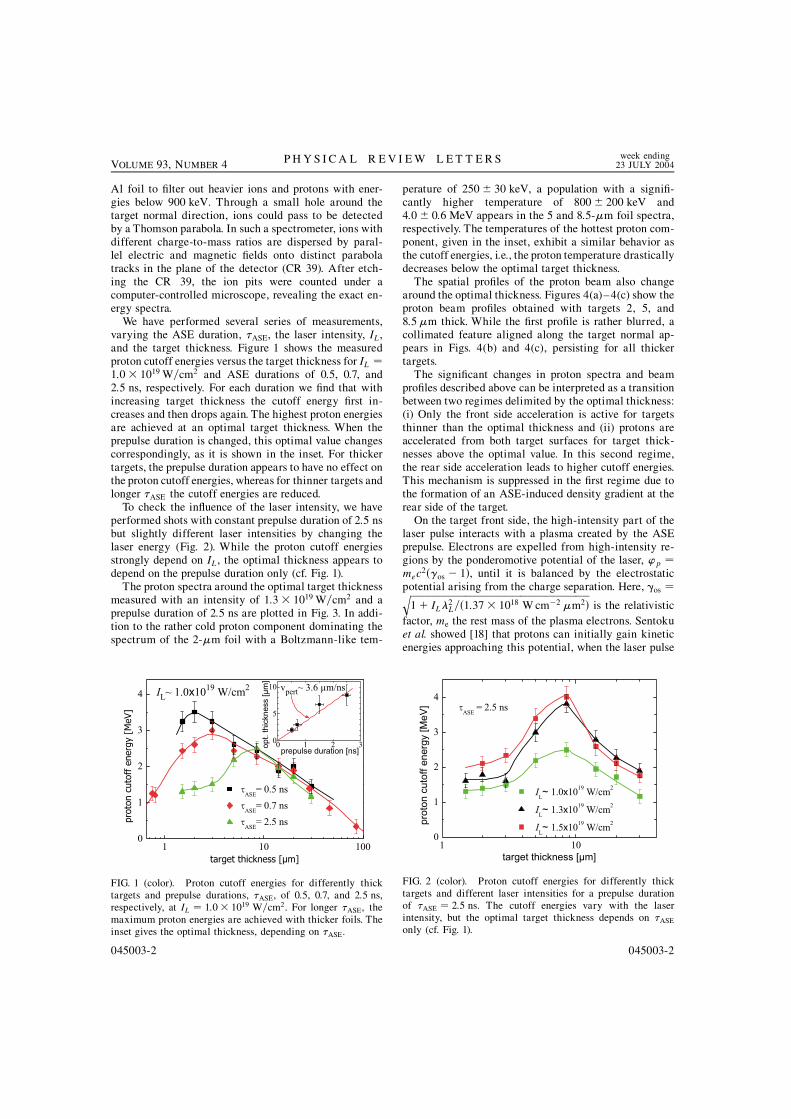
Al foil to filter out heavier ions and protons with ener-gies below 900 keV. Through a small hole around thetarget normal direction, ions could pass to be detectedby a Thomson parabola. In such a spectrometer, ions withdifferent charge-to-mass ratios are dispersed by paral-lel electric and magnetic fields onto distinct parabolatracks in the plane of the detector (CR 39). After etch-ing the CR 39, the ion pits were counted under acomputer-controlled microscope, revealing the exact en-ergy spectra.
We have performed several series of measurements,varying the ASE duration, ASE, the laser intensity, IL,and the target thickness. Figure 1 shows the measuredproton cutoff energies versus the target thickness for IL 1:0 1019 W=cm2 and ASE durations of 0.5, 0.7, and2:5 ns, respectively. For each duration we find that withincreasing target thickness the cutoff energy first in-creases and then drops again. The highest proton energiesare achieved at an optimal target thickness. When theprepulse duration is changed, this optimal value changescorrespondingly, as it is shown in the inset. For thickertargets, the prepulse duration appears to have no effect onthe proton cutoff energies, whereas for thinner targets andlonger ASE the cutoff energies are reduced.
To check the influence of the laser intensity, we haveperformed shots with constant prepulse duration of 2:5 nsbut slightly different laser intensities by changing thelaser energy (Fig. 2). While the proton cutoff energiesstrongly depend on IL, the optimal thickness appears todepend on the prepulse duration only (cf. Fig. 1).
The proton spectra around the optimal target thicknessmeasured with an intensity of 1:3 1019 W=cm2 and aprepulse duration of 2:5 ns are plotted in Fig. 3. In addi-tion to the rather cold proton component dominating thespectrum of the 2-m foil with a Boltzmann-like tem-
perature of 250 30 keV, a population with a signifi-cantly higher temperature of 800 200 keV and4:0 0:6 MeV appears in the 5 and 8:5-m foil spectra,respectively. The temperatures of the hottest proton com-ponent, given in the inset, exhibit a similar behavior asthe cutoff energies, i.e., the proton temperature drasticallydecreases below the optimal target thickness.
The spatial profiles of the proton beam also changearound the optimal thickness. Figures 4(a)–4(c) show theproton beam profiles obtained with targets 2, 5, and8:5m thick. While the first profile is rather blurred, acollimated feature aligned along the target normal ap-pears in Figs. 4(b) and 4(c), persisting for all thickertargets.
The significant changes in proton spectra and beamprofiles described above can be interpreted as a transitionbetween two regimes delimited by the optimal thickness:(i) Only the front side acceleration is active for targetsthinner than the optimal thickness and (ii) protons areaccelerated from both target surfaces for target thick-nesses above the optimal value. In this second regime,the rear side acceleration leads to higher cutoff energies.This mechanism is suppressed in the first regime due tothe formation of an ASE-induced density gradient at therear side of the target.
On the target front side, the high-intensity part of thelaser pulse interacts with a plasma created by the ASEprepulse. Electrons are expelled from high-intensity re-gions by the ponderomotive potential of the laser, ’p mec
2os 1, until it is balanced by the electrostaticpotential arising from the charge separation. Here, os
1 IL2L=1:37 1018 W cm2 m2
q
is the relativistic
factor, me the rest mass of the plasma electrons. Sentokuet al. showed [18] that protons can initially gain kineticenergies approaching this potential, when the laser pulse
FIG. 1 (color). Proton cutoff energies for differently thicktargets and prepulse durations, ASE, of 0.5, 0.7, and 2:5 ns,respectively, at IL 1:0 1019 W=cm2. For longer ASE, themaximum proton energies are achieved with thicker foils. Theinset gives the optimal thickness, depending on ASE.
FIG. 2 (color). Proton cutoff energies for differently thicktargets and different laser intensities for a prepulse durationof ASE 2:5 ns. The cutoff energies vary with the laserintensity, but the optimal target thickness depends on ASE
only (cf. Fig. 1).
P H Y S I C A L R E V I E W L E T T E R S week ending23 JULY 2004VOLUME 93, NUMBER 4
045003-2 045003-2

is longer than the acceleration time a L=c
mp=meos
q
; where mp is the proton mass. For ourconditions, we have a 70 fs, which is shorter thanour pulse duration, and ’p varies between 0.72 and0:92 MeV, depending on IL. During the acceleration, asharp proton front is formed, that expands afterwardsdue to an electrostatic repulsion within this front, addi-tionally increasing the peak proton velocity by 50% [18],and thus resulting in cutoff energies of 1:52 ’p 1:6 . . . 2:1 MeV for protons accelerated at the front sideof the target.
The target normal sheath acceleration (TNSA) mecha-nism is responsible for proton acceleration from the targetrear side [15]. At the front side, a fraction of 25% ofthe laser energy is converted into fast electrons having amean energy of kBTe mec
2os 1 [19], resulting in atotal number Ne EL=kBTe of hot electrons that propa-gate through the target. Arriving at the rear side, only asmall fraction of the fastest electrons can escape, whilethe target charges up. Most of the electrons are held back
by the arising electic field and form a sheath at the rearside with a Debye length of D
"0kBTe=nee2
p
. Thisfield ionizes atoms at the rear surface and acceleratesthem in target normal direction. Mora described theacceleration process with 1D simulations [20]. Here, thetarget consists of preionized hydrogen. The electrons,having a mean energy of kBTe during the laser pulseduration, are assumed to be in thermal equilibrium withthe electrostatic potential at the target rear side, i.e.,ne ne0 expe=kBTe. On the other hand, canbe obtained from the Poisson equation "0@
2=@x2 ene np, taking into account the electron and protondensities. Initially, the proton density, np, is steplike withnp ne0 in the target. By iteratively solving the equationof motion and the continuity equation for the protons,their new density in the next time step is obtained, lead-ing to a new potential and electric field. As the field isalways peaked at the proton front, the fastest protons arealso located there. Mora also found an analytical expres-sion for the evolution of the maximum proton energy, Ep,as a function of the interaction time, ti, depending only onthe electron temperature, Te, and the initial electrondensity, ne0:
Ep 2kBTe
(
ln
"
ti!pp
2eEp
1
ti!pp
2eEp
2s #)
2
: (1)
!pp
ne0e2="0mp
q
is the proton plasma frequency, thatdepends on ne0, and eE 2:71828 . . . .We assume ti L,the same electron numbers and temperatures on bothtarget surfaces, and a constant divergence of the electronbeam propagating through the target. The hot electrondensity at the rear side, ne0, is estimated as follows.Accelerated in the laser focus with an initial radius ofrf 2:5m and a half-opening angle of in, the electronbeam travels through an effective target thickness ofdt dt= cos30 and leaves it within an area of "rf dt tan in2. Assuming an electron bunch length of cL,the averaged electron density at the rear side is
ne0 Ne
cL "rf dt tan in2: (2)
The peak proton energies for differently thick tar-gets calculated with Eqs. (1) and (2) are compared inFig. 5 with the experimental results for IL 1:3 1019 W=cm2 and ASE 2:5 ns. The cutoff energies fortargets optimally thick and thicker are well describedby this model for an initial half-opening angle of in 8 2, which is comparable to the value found in [21].For the same in, this model describes also well the resultsfrom Fig. 1, when the reduced laser intensity is taken intoaccount.
The cutoff energies for thinner targets cannot be ex-plained by the TNSA mechanism assuming a steplikedensity gradient at the rear side. Because of the ASEprepulse, a plasma is formed at the target rear surface,
FIG. 4. Proton beam profiles for ASE 2:5 ns recorded onCR 39 for 2, 5, and 8:5m thick targets, respectively. While in(a) the profile is blurred, we observe in (b) and (c) that themajor part of the beam is well collimated along the targetnormal direction. This collimated feature appears only fortargets at and above the optimal thickness. The circles in (a)give half-opening angles of 5, 10, and 15, respectively.
FIG. 3 (color). Proton spectra at IL 1:3 1019 W=cm2 forASE 2:5 ns and 2, 5, and 8:5m thick foils. With increasingtarget thickness, a second hotter proton population with muchhigher cutoff energies appears. The inset gives the temperaturesof the hot proton component for all measured thicknesses. Asimilar behavior is observed for all different ASE.
P H Y S I C A L R E V I E W L E T T E R S week ending23 JULY 2004VOLUME 93, NUMBER 4
045003-3 045003-3
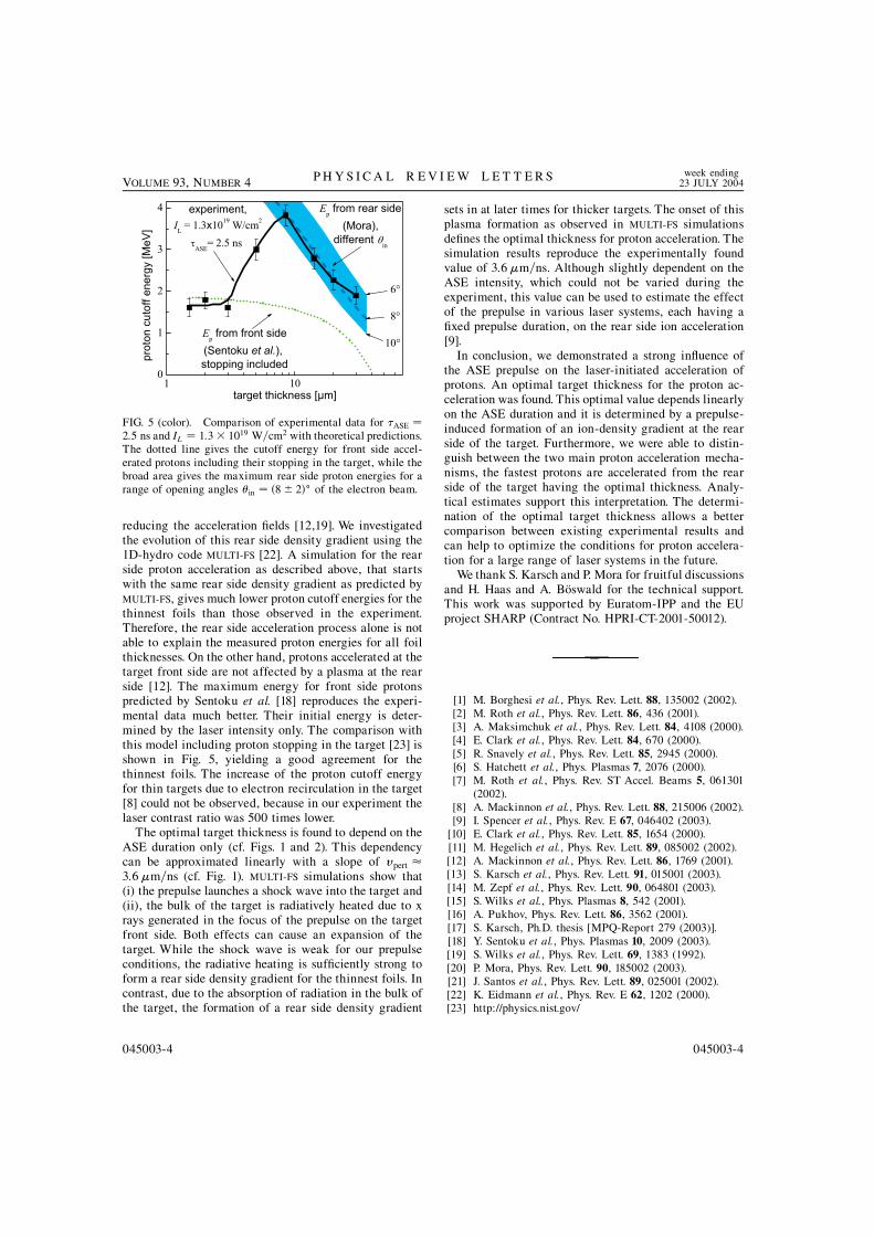
reducing the acceleration fields [12,19]. We investigatedthe evolution of this rear side density gradient using the1D-hydro code MULTI-FS [22]. A simulation for the rearside proton acceleration as described above, that startswith the same rear side density gradient as predicted byMULTI-FS, gives much lower proton cutoff energies for thethinnest foils than those observed in the experiment.Therefore, the rear side acceleration process alone is notable to explain the measured proton energies for all foilthicknesses. On the other hand, protons accelerated at thetarget front side are not affected by a plasma at the rearside [12]. The maximum energy for front side protonspredicted by Sentoku et al. [18] reproduces the experi-mental data much better. Their initial energy is deter-mined by the laser intensity only. The comparison withthis model including proton stopping in the target [23] isshown in Fig. 5, yielding a good agreement for thethinnest foils. The increase of the proton cutoff energyfor thin targets due to electron recirculation in the target[8] could not be observed, because in our experiment thelaser contrast ratio was 500 times lower.
The optimal target thickness is found to depend on theASE duration only (cf. Figs. 1 and 2). This dependencycan be approximated linearly with a slope of vpert 3:6m=ns (cf. Fig. 1). MULTI-FS simulations show that(i) the prepulse launches a shock wave into the target and(ii), the bulk of the target is radiatively heated due to xrays generated in the focus of the prepulse on the targetfront side. Both effects can cause an expansion of thetarget. While the shock wave is weak for our prepulseconditions, the radiative heating is sufficiently strong toform a rear side density gradient for the thinnest foils. Incontrast, due to the absorption of radiation in the bulk ofthe target, the formation of a rear side density gradient
sets in at later times for thicker targets. The onset of thisplasma formation as observed in MULTI-FS simulationsdefines the optimal thickness for proton acceleration. Thesimulation results reproduce the experimentally foundvalue of 3:6m=ns. Although slightly dependent on theASE intensity, which could not be varied during theexperiment, this value can be used to estimate the effectof the prepulse in various laser systems, each having afixed prepulse duration, on the rear side ion acceleration[9].
In conclusion, we demonstrated a strong influence ofthe ASE prepulse on the laser-initiated acceleration ofprotons. An optimal target thickness for the proton ac-celeration was found. This optimal value depends linearlyon the ASE duration and it is determined by a prepulse-induced formation of an ion-density gradient at the rearside of the target. Furthermore, we were able to distin-guish between the two main proton acceleration mecha-nisms, the fastest protons are accelerated from the rearside of the target having the optimal thickness. Analy-tical estimates support this interpretation. The determi-nation of the optimal target thickness allows a bettercomparison between existing experimental results andcan help to optimize the conditions for proton accelera-tion for a large range of laser systems in the future.
We thank S. Karsch and P. Mora for fruitful discussionsand H. Haas and A. Boswald for the technical support.This work was supported by Euratom-IPP and the EUproject SHARP (Contract No. HPRI-CT-2001-50012).
[1] M. Borghesi et al., Phys. Rev. Lett. 88, 135002 (2002).[2] M. Roth et al., Phys. Rev. Lett. 86, 436 (2001).[3] A. Maksimchuk et al., Phys. Rev. Lett. 84, 4108 (2000).[4] E. Clark et al., Phys. Rev. Lett. 84, 670 (2000).[5] R. Snavely et al., Phys. Rev. Lett. 85, 2945 (2000).[6] S. Hatchett et al., Phys. Plasmas 7, 2076 (2000).[7] M. Roth et al., Phys. Rev. ST Accel. Beams 5, 061301
(2002).[8] A. Mackinnon et al., Phys. Rev. Lett. 88, 215006 (2002).[9] I. Spencer et al., Phys. Rev. E 67, 046402 (2003).
[10] E. Clark et al., Phys. Rev. Lett. 85, 1654 (2000).[11] M. Hegelich et al., Phys. Rev. Lett. 89, 085002 (2002).[12] A. Mackinnon et al., Phys. Rev. Lett. 86, 1769 (2001).[13] S. Karsch et al., Phys. Rev. Lett. 91, 015001 (2003).[14] M. Zepf et al., Phys. Rev. Lett. 90, 064801 (2003).[15] S. Wilks et al., Phys. Plasmas 8, 542 (2001).[16] A. Pukhov, Phys. Rev. Lett. 86, 3562 (2001).[17] S. Karsch, Ph.D. thesis [MPQ-Report 279 (2003)].[18] Y. Sentoku et al., Phys. Plasmas 10, 2009 (2003).[19] S. Wilks et al., Phys. Rev. Lett. 69, 1383 (1992).[20] P. Mora, Phys. Rev. Lett. 90, 185002 (2003).[21] J. Santos et al., Phys. Rev. Lett. 89, 025001 (2002).[22] K. Eidmann et al., Phys. Rev. E 62, 1202 (2000).[23] http://physics.nist.gov/
FIG. 5 (color). Comparison of experimental data for ASE 2:5 ns and IL 1:3 1019 W=cm2 with theoretical predictions.The dotted line gives the cutoff energy for front side accel-erated protons including their stopping in the target, while thebroad area gives the maximum rear side proton energies for arange of opening angles in 8 2 of the electron beam.
P H Y S I C A L R E V I E W L E T T E R S week ending23 JULY 2004VOLUME 93, NUMBER 4
045003-4 045003-4

Danksagung
An dieser Stelle mochte ich allen, die zum Gelingen meiner Arbeit beigetragen haben, einganz herzliches Dankeschon aussprechen.
• Besonders danke ich meinem Doktorvater Herrn Prof. Dr. Jurgen Meyer-ter-Vehnfur die außerst kompetente Betreuung der Arbeit, fur dieHilfe bei theoretischenUberlegungen und fur das stete Interesse am Fortgang meiner Arbeit.
• Ich danke Herrn Prof. Dr. Alfred Lauberau fur die bereitwillige Ubernahme desZweitgutachtens.
• Ebenso mochte ich mich bei Herrn Prof. Dr. Klaus-Jurgen Witte fur die herzlicheAufnahme in die Laser-Plasma-Gruppe am MPQ bedanken, sowiefur die zahl-reichen und sehr ausfuhrlichen Diskussionen uber meine Arbeit, die mir sehr ge-holfen und mich zusatzlich motiviert haben.
• Mein besonderer Dank gilt Herrn Dr. Georges D. Tsakiris furdie außerordentlichgute Zusammenarbeit wahrend der gesamten Zeit. Zum einen hat er mich zum wis-senschaftlichen Arbeiten angeleitet, zum anderen hat er mir die notigen Freiraumezum Arbeiten gelassen.
• Ein großes Dankeschon an Herrn Dr. Javier Honrubia fur dieDurchfuhrung dernumerischen Simulationen zum Elektronentransport im Target, die wichtige Erkla-rungen zu den Experimenten liefern konnten.
• Herrn Dr. Klaus Eidmann danke ich fur die geduldige Hilfe bei den Simulationenmit MULTI und MULTI -FS.
• Herrn Dr. Marko Santala und Herrn Jorg Schreiber sei herzlich fur ihre Mitwirkungbeim Experiment, fur die vielen guten Ideen und fur die Unterstutzung bei derAuswertung der Daten gedankt.
• Herrn Dr. Riccardo Tommasini mochte ich fur die Hilfe bei der Berechnung dertheoretischen Intensitatsverteilung im Fokus danken.
• Bei Herrn Matthias Dreher mochte ich mich besonders fur die Hilfe auch bei denkniffeligsten physikalischen und computertechnischen Fragen bedanken aber auchfur alle Diskussionen, die nur im weiteren Sinne mit Physikzu tun hatten.
• Herrn Dr. Stefan Karsch mochte ich fur dieUberlassung seiner Thomson-Parabelzum Experimentieren danken, sowie fur zahlreichen Anregungen zu meiner Arbeit.

• Fur die Mitarbeit im Labor danke ich den Herren Dr. Istvan F¨oldes, Ervin Raczund Dr. Hideaki Habara. Herrn Dr. Michael Jost, Herrn Dr. Michael Geissler, HerrnJurgen Stein, Herrn Dr. Ulrich Andiel, Herrn Dr. Paris Tzallas, Frau Dr. FrancescaPisani, Herrn Prof. Dr. Georg Pretzler, Herrn Dr. Manuel Hegelich, Herrn Dr. ErnstFill, Herrn Dr. Andrius Marcinkevicius, Herrn Felix Brandl und Frau Annika Krenzsei gedankt fur die zahlreichen physikalischen und nicht-physikalischen Gesprache.
• Ich danke den Herren Alois Boswald, Harald Haas und Horst Baumhacker fur denhervorragenden ATLAS-Laserbetrieb. Besonders bei Herrn Haas mochte ich michan dieser Stelle fur die Hilfe beim Einbau und beim Betrieb der schnellen Pockels-zelle bedanken.
• Allen weiteren Mitarbeitern der Laser-Plasma Gruppe, insbesondere den HerrenGunther Keller, Manfred Fischer und Walter Folsner, sowie der gesamten Werk-statt des MPQ gilt mein besonderer Dank fur die Hilfe bei kleineren und großerenmechanischen Problemen.
• Nicht zuletzt danke ich meinen Eltern, meiner Schwester Wiebke und ganz beson-ders naturlich meiner Miri fur den personlichen Ruckhalt wahrend der gesamtenZeit.