characteristics-based marker method with …msi.umn.edu/~lilli/taras-pepi.pdfconcept of the method...
TRANSCRIPT

1
Characteristics-based marker method with conservative finite-differences schemes for
modeling geological flows with strongly variable transport properties
Taras V. Gerya1,2,* and David A. Yuen3
1Institute of Experimental Mineralogy, Russian Academy of Sciences, Chernogolovka,
142432 Moscow, Russia2Institut für Geologie, Mineralogie und Geophysik, Ruhr-Universität Bochum, 44780
Bochum, Germany3Minnesota Supercomputer Institute and Department of Geology and Geophysics, University
of Minnesota, Minneapolis, Minnesota, 55455 USA
Submitted to Physics of the Earth and Planetary Interiors,
December 2002
* Corresponding author. Tel.: +49-234-3223518;
fax: +49-234-3214433.
E-mail address: [email protected] (T. Gerya)

2
Abstract
We have designed a 2-D thermal-mechanical code, incorporating both a characteristics
based marker method and conservative finite-difference schemes. In this paper we will give a
detailed description of this code. The temperature equation is advanced in time with the
Lagrangian marker techniques based on the method of characteristics and the temperature
solution is interpolated back to an Eulerian grid configuration at each timestep. This marker
approach allows for the accurate portrayal of very fine thermal structures. For attaining a high
relative accuracy in the solution of the matrix equations associated with both the momentum
and temperature equations, we have employed the direct matrix inversion technique, which
becomes feasible with the advent of very large shared-memory machines. Our conservative
finite-difference schemes allow us to capture sharp variations of the stresses and thermal
gradients in problems with a strongly variable viscosity and thermal conductivity. We have
tested this code with numerous examples drawn from Rayleigh-Taylor instabilities, the
descent of a stiff object into a medium with a lower viscosity, viscous heating and flows with
non-Netwonian rheology. We have also benchmarked successfully with variable viscosity
convection for lateral viscosity contrast up to 108. We have delineated the regions in thermal
problems where the diffusive nature of the temperature equation changes from its parabolic
character locally to a non-linear hyperbolic-like equation due to the presence of variable
thermal conductivity. Finally we discuss the applicability of this marker-based and finite-
difference technique to other evolutionary equations in geophysics.
Keywords: mantle convection; finite-differences; Eulerian/Lagrangian approach; marker
method; shared-memory
3
1. Introduction
Today, as modeling of geomechanics is entering a new millennium, geoscientists are
faced with more realistic situations in lithospheric and mantle dynamics. These new
difficulties arise from the need to model with great fidelity the significant finite deformation
in strongly viscous rocks at cold temperatures to contrasting rheological properties across
fault zones (Kameyama et al, 1999, Regenauer-Lieb et al., 2001; Kameyama and Kaneda,
2002) and transport properties involving vapor or volatiles (e.g. Woods, 1999; Richard et al.,
2002). The rheology of crustal and mantle rocks depends strongly on the temperature, strain-
rate, volatile content, grain size and the hydrostatic pressure (e.g. Ranalli, 1995; Karato,
1997). These extenuating physical and dynamical circumstances imposed by the sharply
varying viscosity and volatiles indeed represent a major challenge for the momentum equation
in geodynamics, unlike those found in the oceanographic or atmospheric sciences. In the limit
of creeping flow or the zero Reynolds number regime, the momentum equation becomes a
highly nonlinear elliptic partial differential equation primarily because of non-linear
constitutive relatisonhsip between the stress and strain-rate tensors, unlike the other areas in
fluid mechanics (e.g. Batchelor, 1967; Balmforth and Provenzale, 2001). The solution of
these elliptic partial differential equations has remained a chief computational challenge in
solid-earth geophysics (Yuen et al., 2000a, b) because of the ill-conditioned nature of the
matrix with vastly varying magnitude in the elements due to the large variations in the
rheological properties of rocks. Various types of methods have been devised for solving the
elliptic equation for variable viscosity. A popular method has been the multigrid method
(Wessling, 1992; Moresi and Solomatov, 1995). Another nonlinearity, not often appreciated
up to now in geomechanical-modelling, is that due to variable thermal conductivity in the
energy equation. The thermal conductivity of crustal and mantle rocks depends on the
temperature and pressure (Hofmeister, 1999) and endows the temperature equation with a
strong nonlinearity from the square of the ∇T term near the boundary layers (Dubuffet and
Yuen, 2000; Dubuffet et al., 2000, 2002) which greatly exacerbates numerical difficulties,
produces numerical instabilties and requires more grid points than for constant thermal
conductivity situations (van den Berg et al., 2001). All transport properties of rocks including
viscosity, conductivity vary strongly with chemical composition or mineralogy. Similar types
of quadractic nonlinearity involving the gradient of volatile content, are also found in
convection equations with volatile or vapor transport (e.g. Woods, 1999; Richard et al., 2002)
Thus they cause sharp fronts involving multicomponent flows in geological situations,
especially when the transport of volatiles is also included in the governing equations in mantle
convection (Fountaine et al, 2001; Richard et al., 2002).

4
From a general geophysical standpoint, we should consider at least three important
elements for modelling these kinds of flows:
(1.) the ability to conserve stresses under conditions involving sharply discontinuous
viscosity distribution;
(2.) the ability to conserve heat and chemical fluxes in the face of sharply varying
conductivity, transport coefficient and temperature gradients at the thermal or chemical
boundary layers with temperature-dependent conductivity and nonlinear transport coefficient,
such as in vapor flow at mid-ocean ridges (Fountaine et al., 2001);
(3.) the ability to conserve scalar quantities with multiscale properties, such as
temperature field, chemical species, and density in flows with a strongly advection character,
i.e. high Peclet number.
Besides these factors, there are other challenges which are also quite potent, such as
phase transitions and its rheological consequences of a dramatic softening from grain-size
reduction from nucleation processes in phase transformation (e.g. Riedel and Karato, 1997).
We aim to demonstrate in this work that all of these requirements can be achieved by using a
conservative finite-difference (FD) scheme with an arbitrary order in accuracy, an
Eulerian/Lagrangian primitive variable formulation based on moving markers which combine
both the control volume method (e.g. Albers, 2000) and the accurate trajectories behind the
concept of the method of characteristics (Malevsky and Yuen, 1991).
Recent advances in hardware technology with the distributed-shared-memory architecture
on supercomputers have prompted us to look again at direct solvers, such as the Gaussian
elimination or Cholesky decomposition (Malevsky and Yuen, 1992) for 2-D problems
because of its prowess in terms of superior relative accuracy over iterative solvers used in
many variable viscosity codes (e.g. Moresi and Solomatov, 1995, Tackley, 1996). Recent
innovations in the machine architecture on the IBM-SP4, CRAY-1X and the Japanese NEC
machines have put at least 16 Gbytes of shared memory available on a single node. Within the
next two years the next generation of these machines will offer 64 to 128 Gbytes on a single
node! It is therefore our challenge to prepare for the onslaught of these ultra-lage distributed-
shared-memory architecture. The anticipation of these coming technological innovations has
figured prominently in our computational strategy laid out in this paper.
In section 2 we will provide in some details the implementation of these algorithms on
conservative finite-difference schemes for modeling flows with variable viscosity and
conductivity. We then move to a description of the marker scheme combined with this
conservative finite-difference method and the novel treatment of the temperature equation by
this hybrid scheme combining the best of the Lagrangian and Eulerian approaches. We then

5
demonstrate in section 3 by some benchmarks the efficacy of our hybrid method and present
the results on various types of flows characterized by variable viscosity, viscous heating and
variable thermal conductivity. The final section will be our discussion and conclusions.
2. Basic background of the numerical modeling scheme
2.1. Principal equations
In this section we will describe in detail the numerical implementation of the fundamental
conservation equations of mass, momentum and energy and the constitutive relationships
between stress and strain-rate needed for modeling geomechanical problems in the two-
dimensional creeping flow regime. They will be applicable in convective heat-transfer
problems involving multiphase viscous fluids in the presence of a gravitational body force
term. This set of partial differential equations comprises, first of all, the Stokes equations of
slow flow where the inertial terms are dropped. Equations (1) and (2) are the second-order
elliptic equations in the velocity field (v).
∂σxx /∂x + ∂σxz /∂z = ∂P/∂x - ρ(T,C)gx, (1)
∂σzz /∂z + ∂σxz /∂x = ∂P/∂z - ρ(T,C)gz. (2)
σxx = 2ηεxx
σxz = 2ηεxz
σzz = 2ηεzz
εxx = ∂vx/∂x
εxz = ½(∂vx/∂z+∂vz /∂x)
εzz = ∂vz/∂z
This is followed by the constitutive relationship between the stress (σ) and strain-rate (ε),
where the transport coefficient η represents the viscosity, which depends on the temperature
(T), pressure (P), volatiles (C) and strain-rate.
The conservation of mass is given by the continuity equation in which we keep density to
be a constant in all terms except for the buoyancy force, where both temperature and volatile
content come into play. This level of truncation is known as the Boussinesq approximation on
which most mantle convection codes were built on (e.g. Moresi and Solomatov, 1995;
Trompert and Hansen, 1996; Albers, 2000)
∂vx/∂x + ∂vz/∂z = 0. (3)
As part of our new computational strategy, instead of using the Eulerian frame of
reference, we have elected to go to the Lagrangian frame of reference in which the
temperature equation takes the form, and the extended Boussinesq approximation

6
(Christensen and Yuen, 1985) has been used to take into account adiabatic and viscous
heating contributions. These two terms are deemed significant in many important tectonic
situations, such as mountain-belt collision (Kincaid and Silver, 1996). The temperature
equation (eqn. 4) is a second-order in space and first-order in time and it is nonlinear in T
because of the variable thermal conductivity.
ρCp(D T/D t) = ∂qx/∂x + ∂qz/∂z + Hr + Ha + Hs, (4)
qx = k(T,P)×(∂T/∂x),
qz = k(T,P)×(∂T/∂z),
Hr = const,
Ha = Tα[vx(∂P/∂x) + vz(∂P/∂z)] ≈ Tαρ[vxgx + vzgz],
Hs = σxxεxx + σzzεzz + 2σxzεxz,
where D/D t represents the substantive time derivative and we have used markers here to
follow the temporal development of both the temperature field and the volatile field, as they
are being advected by the common velocity field. Other notations in equations (1)-(4) are: x
and z denotes, respectively, the horizontal and vertical coordinates, in m, vx and vz are
components of the velocity vector in m⋅s-1; t time in s; σxx, σxz, σzz are components of the
viscous deviatoric stress tensor in units of Pa; εxx, εxz, εzz are components of the strain rate
tensor in s-1; P the pressure in Pa; T the temperature in K; qx and qz are horizontal and vertical
heat flows in W⋅m-2; η the effective viscosity in Pa⋅s, depending on pressure, temperature and
strain rate (e.g. Ranalli, 1995); ρ the density in kg⋅m-3, depending on chemical composition,
phase assemblage (e.g. presence of dense minerals, melt, e.g. Gerya et al., 2001, 2002),
pressure and temperature; gx and gz denote components of the vector of acceleration within
the gravity field for the x-z 2-D coordinate system (deviation of this vector from vertical
direction may become important for very large scale mantle convection models), m⋅s-2; k(T,P)
is the variable thermal conductivity coefficient in W⋅m-1⋅K-1, depending on the temperature
and pressure; Cp is the isobaric heat capacity in J⋅kg-1⋅K-1; Hr, Ha, and Hs denote, respectively,
radioactive, adiabatic and shear heating production in W⋅m-3 (for simplicity of calculation of
Ha slight deviations of dynamic pressure gradients ∂P/∂x and ∂P/∂z from ρgx and ρgz values
are neglected).
2.2 Computational strategy with markers
In order to achieve the goals set out in geo-modelling as outlined in the introduction, we
have designed a conservative finite-difference (FD) scheme over an irregularly-spaced
staggered grid in a Eulerian grid configuration (Fig. 1). The irregularly spaced grid is
7
extremely useful in handling geodynamical situations with multiple-scale character, such as in
a subducting slab and the wedge flow above it (e.g. Davies and Stevenson, 1992). This
Eulerian FD method is then combined with the moving marker technique or the Lagrangian
approach, shown in Fig. 2, to solve equations (1) to (4). We show in Fig. 3 a schematic flow-
chart for updating at each timestep the evolutionary equations contained in (1) to (4). We have
solved equations (1) to (4) based on a combination of finite control volume method (e.g.
Patankar, 1980; Albers, 2000), combined with an arbitrary order of accuracy in the finite-
difference (FD) discretization (Fornberg, 1995) and method of characteristics (e.g. Malevsky
and Yuen, 1991; De Smet et al., 2000) implemented via the moving marker technique (e.g.
Hockney and Eastwood, 1981; Christensen and Yuen, 1984; Weinberg and Schmeling, 1992;
Schott and Schmeling, 1998; Gerya et al., 2000). The steps are as follows:
(1) Solving 2-D equations (1) to (3) by directly inverting the global matrix with a
Gaussian elimination method, which is chosen because of its programming simplicity,
stability and high accuracy.
(2) Calculating the nonlinear shear- and adiabatic heating terms Hs(i,j) and Ha(i,j) at the
Eulerian nodes.
(3) Advancing (D T/D t)(i,j) in time at the Eulerian nodes by a first-order explicit
scheme.
(4) Defining an optimal time step ∆t for temperature equation. We use a minimum time
step value satisfying the following conditions: given absolute time step limit; given relative
marker displacement step limit (typically 0.1-0.2 of minimal grid step) corresponding to
calculated velocity field (see Step 1); given absolute nodal temperature change limit
(typically 1-20 K) corresponding to calculated explicit (D T/D t)(i,j) values (see Step 3).
(5) Solving the nonlinear temperature equation implicitly by a direct Gaussian
inversion method.
(6) Interpolating calculated nodal temperature changes (see Step 6 at Fig. 3) from the
Eulerian nodes to the markers and calculating new marker temperatures (tTm).
(7) Using a fourth-order explicit Runge-Kutta scheme for advecting all markers
throughout the mesh according to the globally calculated velocity field v (see Step 1).
(8) Calculating globally the scalar physical properties (ηm, ρm, Cm, Cpm, km, C, etc.)
from the markers.
(9) Interpolating temperature and other scalar properties, such as C, Cp, from the
markers to Eulerian nodes. Returning to Step 1 at the next timestep.
We have implemented the above computational algorithm in a new computer code, called
12VIS, which is written in the C- computer language in order to facilitate post-processing.
8
This code has been developed on the basis of our previous thermo-mechanical code based on
finite-differences, (I2), which employed finite-difference method over a half-staggered grid
and used the marker technique (Gerya et al., 2000).
2.3. Interpolation of scalar fields, vectors and tensors
According to our algorithmic approach the temperature field and other scalar properties
(η, ρ, Cp, C, k, etc.) are represented by scalar values ascribed for the multitudinous markers
initially distributed on a fine regular marker mesh with a small (≤ ½ of marker grid distance)
random displacement (Fig.2). The effective values of all these parameters at the Eulerian
nodal points are interpolated from the markers at each time step. The following standard first
order of accuracy scheme (e.g. Fornberg, 1995) is used to calculate an interpolated value of a
parameter B(i,j) for ijth-node using values (Bm) ascribed to all markers found in the four
surrounding cells (Fig. 2a)
B(i,j) = ∑m
j)m(i,m wB / ∑m
j)m(i,w , (5)
wm(i,j) = [1-∆xm/∆x(i-½)]×[1-∆zm/∆z(j-½)]/[∆x(i-½)×∆z(j-½)],
where wm(i,j) represents a statistical weight of mth-marker at the ijth-node; ∆xm/∆x(i-½) and
∆zm/∆z(i-½) are normalized distances from mth-marker to ijth-node. In the case of non-uniform
Eulerian grid, we use a two-dimensional bisectioning method to determine the corresponding
grid cell in which the marker is located (Fig 2a). For interpolating the nodes along the
margins we use only the markers found inside an Eulerian grid independent of the boundary
conditions. The slight inaccuracy of interpolation for marginal nodes is compensated by our
increasing the grid resolution at the boundaries. The use of a higher-order accurate
interpolation schemes produces undesirable numerical fluctuations in scalar, vector and tensor
properties interpolated in the proximity of sharp transitions. For example, negative values of
viscosity are calculated at the fixed Eulerian nodes at thermal boundary layers with sharp
(>103) viscosity contrast, by using a second order FD scheme (e.g. Fornberg, 1995).
For the same reason we have used a standard first order of accuracy (e.g. Fornberg, 1995)
procedure for the reversed problem of interpolating the scalar properties (including calculated
temperature changes), vectors and tensors from the corresponding Eulerian nodal points (see
different types of Eulerian nodes in Fig. 1) back to the markers and other geometrical points
(e.g. other nodes). The values of a parameter B defined in four Eulerian nodes surrounding a
given marker (Fig. 2b) are used for calculating an effective value of the parameter B for mth-
marker as follows
Bm = [1-∆xm/∆x(i-½)]×[1-∆zm/∆z(j-½)]×B(i,j) + [∆xm/∆x(i-½)]×[1-∆zm/∆z(j-½)]×B(i-1,j) +

9
[1-∆xm/∆x(i-½)]×[∆zm/∆z(j-½)]×B(i,j-1) + [∆xm/∆x(i-½)]×[∆zm/∆z(j-½)]×B(i-1,j-1), (6)
where Bm denote the value of parameter B for mth-marker. Scheme (6) is used uniformly,
when we interpolate the velocity, stresses, strain rates, pressure, temperature and other
properties from nodal points to markers. Since our staggered grid represents, in fact, the
superposition of four simple rectanugular grids corresponding to different scalar fields,
vectors and tensor (see four different symbols for gridpoints in Fig 1), these Eulearian grids
are used individually for interpolating the respective field variables.
The standard first-order interpolation schemes yield equally good results in cases (1)-(4)
comparing to more complex, higher-order (e.g. Fornberg, 1995) interpolation schemes.
2.4. Finite-difference schemes for discretizing the momentum and continuity equations
The following FD scheme is a discretized form for representing equations (1), (2) and (3)
to a first order accuracy in the control volume representation (e.g. Albers, 2000), which
allows for the conservation of the viscous stresses between the nodal points (see Fig. 1 for the
indexing of the grid points):
[∂σxx /∂x](i,j+½) + [∂σxz /∂z](i,j+½) - [∂P/∂x](i,j+½) = - ½[ρ(i,j)+ρ(i,j+1)]×gx(i,j+½) (7)
[∂σxx /∂x](i,j+½) = 2[σxx(i+½,j+½) - σxx(i-½,j+½)]/[∆x(i-½)+∆x(i+½)],
[∂σxz /∂z](i,j+½) = [σxz(i,j+1) - σxz(i,j)]/∆z(j+½),
[∂P/∂x](i,j+½) = 2[P(i+½,j+½) - P(i-½,j+½)]/[∆x(i-½)+∆x(i+½)],
where i, i+½ and j, j+½ indexes denote, respectively, the horizontal and vertical positions of
nodal points corresponding to the different physical parameters (Fig. 1) within the staggered
grid (Wessling, 1992).
[∂σzz /∂z](i+½,j) + [∂σxz /∂x](i+½,j) - [∂P/∂z](i+½,j) = - ½[ρ(i,j)+ρ(i+1,j)]×gz(i+½,j), (8)
[∂σzz /∂z](i+½,j) = 2[σzz(i+½,j+½) - σzz(i+½,j-½)]/[∆z(j-½)+∆z(j+½)],
[∂σxz /∂x](i+½,j) = [σxz(i+1,j) - σxz(i,j)]/∆x(i+½),
[∂P/∂z](i+½,j) = [P(i+½,j+½) - P(i+½,j-½)]/[∆z(j-½)+∆z(i+½)],
and
[∂vx/∂x](i-½,j-½) + [∂vz/∂z](i-½,j-½) = 0; (9)
where
σxx(i-½,j+½) = ½[η(i-1,j)+η(i-1,j+1)+η(i,j)+η(i,j+1)]×εxx(i-½,j+½)
σxx(i+½,j+½) = ½[η(i,j)+η(i,j+1)+η(i+1,j)+η(i+1,j+1)]×εxx(i+½,j+½)
σxz(i,j) = 2η(i,j)εxz(i,j),
σxz(i,j+1) = 2η(i,j+1)εxz(i,j+1),

10
σxz(i+1,j) = 2η(i+1,j)εxz(i+1,j),
σzz(i+½,j-½) = ½[η(i,j-1)+η(i,j)+η(i+1,j-1)+η(i+1,j)]×εzz(i+½,j-½)
σzz(i+½,j+½) = ½[η(i,j)+η(i,j+1)+η(i+1,j)+η(i+1,j+1)]×εzz(i+½,j+½)
εxx(i-½,j+½) = [∂vx/∂x](i-½,j+½)
εxx(i+½,j+½) = [∂vx/∂x](i+½,j+½)
εxz(i,j) = ½[∂vx/∂z+∂vz/∂x](i,j),
εxz(i,j+1) = ½[∂vx/∂z+∂vz/∂x](i,j+1),
εxz(i+1,j) = ½[∂vx/∂z+∂vz/∂x](i+1,j),
εzz(i+½,j-½) = [∂vz/∂z](i+½,j-½)
εzz(i+½,j+½) = [∂vz/∂z](i+½,j+½)
In the FD formulation of equations (7) and (8) the stress is decomposed into a product of
the viscosity and the strain-rate. The latter is formulated, using an arbitrary order accurate FD
scheme (Fornberg, 1995) for the derivatives of velocity. This formulation is also used in finite
difference treatment of seismic wave propagation (Virieux, 1986). First-order accurate FD
scheme for these derivatives most suitable for problems with sharply varying viscosity are
written as
[∂vx/∂x](i-½,j-½) = [vx(i,j-½) - vx(i-1,j-½)]/∆x(i-½),
[∂vx/∂x](i-½,j+½) = [vx(i,j+½) - vx(i-1,j+½)]/∆x(i-½),
[∂vx/∂x](i+½,j+½) = [vx(i+1,j+½) - vx(i,j+½)]/∆x(i+½),
[∂vx/∂z](i,j) = 2[vx(i,j+½) - vx(i,j-½)]/[∆z(j-½)+∆z(j+½)],
[∂vx/∂z](i,j+1) = 2[vx(i,j+1½) - vx(i,j+½)]/[∆z(j+½)+∆z(j+1½)],
[∂vx/∂z](i+1,j) = 2[vx(i+1,j+1½) - vx(i+1,j-½)]/[∆z(j-½)+∆z(j+½)],
[∂vz/∂x](i,j) = 2[vz(i+½,j) - vz(i-½,j)]/[∆x(i-½)+∆x(i+½)],
[∂vz/∂x](i,j+1) = 2[vz(i+½,j+1) - vz(i-½,j+1)]/[∆x(i-½)+∆x(i+½)],
[∂vz/∂x](i+1,j) = 2[vz(i+1½,j) - vz(i+½,j)]/[∆x(i+½)+∆x(i+1½)],
[∂vz/∂z](i-½,j-½) = [vz(i-½,j) - vz(i-½,j-1)]/∆z(j-½),
[∂vz/∂z](i+½,j-½) = [vz(i+½,j) - vz(i+½,j-1)]/∆z(j-½),
[∂vz/∂z](i+½,j+½) = [vz(i+½,j+1) - vz(i+½,j)]/∆z(j+½),
We invert for the global matrix by a highly accurate, direct (Gaussian) method for the
simultaneous solution of momentum equations (7),(8) and continuity equation (9) also
combined with linear equations describing the boundary conditions for the velocity. We
would like to emphasize that continuity equation (9) with the velocity vectors as the variables
is solved directly to machine accuracy with the direct matrix inversion method, thus obviating
the usual need of using the streamfunction formulation. In what follows, the momentum

11
equations (7) and (8) are solved for vx(i,j+½) and vz(i+½,j), respectively, while the continuity
equation (9) is solved for P(i-½,j-½). Incompressible continuity equation (9) does not initially
contain P(i-½,j-½) and the solution is guaranteed by the order of processing during the inversion
of the global matrix (see Fig. 1 for indexing): equation (9) for pressure in a given cell (e.g. P(i-
½,j-½), see Fig. 1), is processed after equations (7) and (8) for all surrounding vx and vz nodes
(e.g. vx(i-1,j-½), vx(i,j-½), vz(i-½,j-1) and vz(i-½,j), see Fig. 1). The relative accuracy of solving the
momentum and continuity equations commonly vary from 10-15 to 10-13.depending on the
viscosity variations. However, in several cases lower (10-6) accuracy has been obtained, as a
result of strong sharp variations in the viscosity (e.g. for some models with ≥106 viscosity
contrast for the adjacent nodes).
2.5. Numerical techniques for solving temperature equation
Malevsky and Yuen (1991) developed a characteristics-based method for solving the
temperature equation to avoid the numerical oscillations from advection at the high Rayleigh
number regime. This method, however, requires an increasing amount of operations for
tracing characteristics back to an initial temperature distribution in the case of strongly
chaotic advection pattern. To avoid this problem, we have implemented a characteristics
based marker technique commonly used for advection of material field properties, such as the
density, viscosity, chemical composition etc. (e.g. Hockney and Eastwood, 1981; Weinberg
and Schmeling, 1992; Schott and Schmeling, 1998; De Smet et al., 2000; Gerya et al., 2000).
According to this approach the temperature field is represented by temperature values (Tm)
assigned for the multitudinous markers initially distributed on a fine marker mesh (see section
2.3). The effective temperature T(i,j) field at the Eulerian nodes is then interpolated from the
markers at each time step, using relation (5). The effective temperatures at the boundary
nodes are then calculated by applying the thermal boundary conditions.
The calculation of the temporal changes in the temperature at the Eulerian nodes is based
on the following implicit first order FD scheme representing equation (4) in a conservative
(e.g. Oran and Boris, 1987) form:
ρ(i,j)Cp(i,j)[D T/D t](i,j)- [∂qx/∂x](i,j) - [∂qz/∂z](i,j) = Hr(i,j) + Ha(i,j) + Hs(i,j), (10)
[D T/D t](i,j) = [1T(i,j) – T(i,j)]/∆t,
[∂qx/∂x](i,j) = 2[1qx(i+½,j) - 1qx(i-½,j)]/[∆x(i-½)+∆x(i+½)],
[∂qz/∂z](i,j) = 2[1qz(i,j+½) - 1qx(i,j-½)]/[∆z(j-½)+∆z(j+½)],1qx(i-½,j) = ½[k(i-1,j)+k(i,j)]×[∂(1T)/∂x](i-½,j);
1qx(i+½,j) = ½[k(i,j)+k(i+1,j)]×[∂(1T)/∂x](i+½,j);1qz(i,j-½) = ½[k(i,j-1)+k(i,j)]×[∂(1T)/∂z](i,j-½);

12
1qz(i,j+½) = ½[k(i,j)+k(i,j+1)]×[∂(1T)/∂z](i,j+½);
Ha(i,j) = T(i,j)α(i,j)ρ(i,j)[vx(i,j)gx(i,j) + vz(i,j)gz(i,j)];
Hs(i,j) = σxx(i,j)εxx(i,j) + σzz(i,j)εzz(i,j) + 2σxz(i,j)εxz(i,j);
where indexes 1 denote values for the next time instant to be reached by the time-stepping and
∆t is the optimal time step (see above, in the section 2.2); Hr(i,j), Ha(i,j), Hs(i,j), α(i,j), ρ(i,j), Cp(i,j),
σxx(i,j), εxx(i,j), σzz(i,j), εzz(i,j), σxz(i,j), εxz(i,j), vx(i,j), and vz(i,j) are values of the corresponding parameters
for the ij-node: scalar properties are interpolated from the markers using relation (5), vectors
and tensors are also interpolated from the corresponding surrounding nodes from equation (6).
In the FD formulation of equation (10) the heat fluxes are decomposed into a product of the
thermal conductivity and the temperature gradients. These quantities are formulated by using
an arbitrary order accurate method FD (Fornberg, 1995) for the derivatives of the temperature.
First-order accurate FD schemes for these derivatives most suitable for problems with
strongly varying thermal conductivity are
[∂(1T)/∂x](i-½,j) = [1T(i,j) - 1T(i-1,j)]/∆x(i-½);
[∂(1T)/∂x](i+½,j) = [1T(i+1,j) - 1T(i,j)]/∆x(i+½)
[∂(1T)/∂z](i,j-½) = [1T(i,j) - 1T(i,j-1)]/∆z(j-½);
[∂(1T)/∂z](i,j+½) = [1T(i,j+1) - 1T(i,j)]/∆z(j+½).
For solving the temperature equations with nonlinearities present we invert directly by a
global matrix with a high accuracy direct (Gaussian) method. The matrix also contains the
linear equations associated with the thermal boundary conditions. The relative accuracy of the
inverted solution spans between 10-15 and 10-13. The changes in the effective temperature field
for the Eulerian nodes are calculated as
∆T(i,j) = [1T(i,j) – T(i,j)]. (11)
Correspondent temperature increments for markers ∆Tm are then interpolated from the nodes
using relation (6) in order to calculate new marker temperatures tTm astTm = Tm + ∆Tm. (11a)
The interpolation of the calculated temperature changes from the Eulerian nodal points to
the moving markers prevents effectively the problem of numerical diffusion. This feature
represents one of the highlights of our computation strategy for solving the temperature
equation using markers. This method does not produce any smoothing of the temperature
distribution between adjacent markers (Fig. 3, diagram for step 6), thus resolving the thermal
structure of a numerical model in much finer details. However, in case of strong chaotic
mixing of markers, our method may produce numerical oscillations of thermal field ascribed
to the adjacent markers. These oscillations do not damp out with time on a characteristic heat

13
diffusion timescale. In order to remove them, we use a weak numerical diffusion occurring
over a characteristic heat diffusion timescale. This is implemented by correcting the marker
temperatures tTm according to the relationtTm(D) = 1Tm – [1Tm – tTm]×exp{–kmd∆t[2/(∆x(i-½))2+2/(∆z(j-½))2]/(Cpmρm)}, (12)
where tTm(D) is mth-marker temperature corrected for the numerical diffusion; d is
dimensionless numerical diffusion coefficient (we use empirical values in the range of
0≤d≤1); 1Tm, Cpm, ρm and km are interpolated, respectively, from 1T(i,j), Cp(i,j), ρ(i,j) and k(i,j)
values for nodes using the relation (6). Complementary (antidiffusion) temperature
corrections ∆T(i,j)A are first calculated at the Eulerian nodes according to relation (5) as
∆T(i,j)A = ∑m
j)m(i,mt
mt wT-T )( D / ∑
mj)m(i,w . (13)
These corrections are then used for complementary (antidiffusion) correction of temperatures
for markers by using relation (6) as followstTm(D-A) = Tm(D) - ∆Tm(A). (13a)
where tTm(D-A) is the final corrected mth-marker temperature; ∆Tm(A) is antidiffusion
temperature correction interpolated for mth-marker from ∆T(i,j)A values for Eulerian nodes
using relation (6). Introducing the numerical diffusion removes the small scale numerical
oscillations over the characteristic heat diffusion timescale and (has been compensated by the
antidiffusion) does not significantly influence the accuracy of numerical solution of the
temperature equation (see section 3.8).
3. Verification of the numerical schemes by calibrating various cases
In this section we will displayed results taken from carrying out several calibrating tests
of the numerical solutions in order to verify the efficacy of our methods for a variety of
circumstances relevant to geothermo-mechanics. These will include
a) sharply discontinuous viscosity distribution (test 1 and 2);
b) strain rate dependent viscosity (test 3);
c) non-steady development of temperature field (test 4);
d) shear heating for temperature dependent viscosity (test 5);
e) advection of a sharp temperature front (test 6);
f) heat conduction for temperature-dependent thermal conductivity (test 7);
g) thermal convection with a large viscosity contrast in the temperature-dependent
viscosity and for both constant and temperature-dependent thermal conductivity (tests
8 and 9).

14
3.1. Rayleigh-Taylor instabilities involving a two-layer cross-section and gravity
A series of tests have been carried out for a two-layer model with a non-slip condition on
the top and at the bottom and symmetry conditions along the vertical walls. An initial
sinusoidal disturbance of the boundary between the upper (η1, ρ1) and the lower (η2, ρ2) layer
of thickness h has a small amplitude (y) and a wave length (λ). This produces favorable
conditions for studying the velocity of the diapiric growth (vz) given by the relation (Ramberg,
1981)
K = 2vzη2/[y(ρ1-ρ2)⋅h⋅g], (14)
where K is a dimensionless factor of growth. Figure 4 compares both the numerical and
analytical solutions for the factor of growth of the diapir estimated at different values of y, λ
and η1/η2. Good accuracy of ±2-5% is determined at large variations of the disturbance wave
length and the layers viscosity contrasts (η1/η2=10-6-5×102). This result shows the correct
numerical solutions of equations (1)-(3) in the case of sharp changes in density and viscosity
across a boundary layer.
3.2. Sinking of a hard rectangular block into a medium with a lower viscosity.
The results of this test are displayed in Figure 5. According to our physical intuitions, the
deformation of the block vanish with increasing viscosity contrast and dynamics of sinking at
high viscosity contrast does not depend on the absolute value of the viscosity of the block.
This test proves the accurate conservation properties of our numerical procedure in terms of
preserving the geometry at large deformation and high (102-106) viscosity contrast between
the harder block and the softer surroundings.
3.3. Channel flow with non-Newtonian rheology
This test is conducted to check the numerical solution of equations (1)-(3) for flows with
a strong strain-rate dependent rheology, which is characterisic of dislocation creep (Ranalli,
1995). The computation is carried out for vertical flow of a viscous non-Newtonian (with a
power-law index n = 3) medium in a channel of the width L in the absence of gravity.
Boundary conditions are taken as follows: for a given vertical pressure gradient, ∂P/∂z, along
the channel and non-slip conditions at the walls. The viscosity of the non-Newtonian flow is
defined by the following rheological equation
σxz = M(∂vz /∂x)1/3, (15)

15
where M is rheological constant in Pa⋅s1/3. The analytical solution for the horizontal profile of
vertical velocity vz and effective strain-rate dependent viscosity η=σxz/(∂vz /∂x) across the
channel is derived from the equations (2) and (15) as follows
vz = vz0[1 - (2x/L - 1)4], (16)
η = η0/(2x/L - 1)2, (17)
vz0 = - L4 [(∂P/∂z)/M]3/64,
η0 = 4M3/[(∂P/∂z)L]2,
where vz0 is the velocity in the center of the channel, η0 is the viscosity at the walls. Figure 6
compares the numerical and analytical solutions for the horizontal distribution of velocity and
viscosity across the channel. We can see clearly that the numerical and analytical solutions
accord quite well, suggesting that our numerical procedure can solve correctly the momentum
equation in the case of strain-rate dependent nonlinear rheology with n = 3.
3.4. Non-steady temperature distribution in a Newtonian channel flow
This time-dependent test is performed to ascertain the numerical accuracy of the
temperature equation (4) in the temporal development (heat advection coupled with heat
diffusion). The calculations are carried out by using a model of the vertical flow of a heat-
conductive medium of constant viscosity in a channel in the absence of gravity. Boundary
conditions are taken as follows: given vertical pressure gradient, ∂P/∂z, along the channel,
non-slip conditions and T=const and ∂T/∂z=const at the walls. The initial conditions are T=To
and ∂T/∂x=0. The horizontal steady-state profile for vertical velocities, vz, is defined by the
equation
vz = 4vzo(Lx - x2)/L2, (18)
vz0 = -L2(∂P/∂z)/(8η),
where L is the width of the channel; η is the viscosity of the channel; vz0 is the vertical
velocity in the center of the channel. The corresponding temperature changes in the channel as
a function of time are given by the following series expansion (Tikhonov and Samarsky,
1972; Gerya et al., 2000)
∆T(x, t) = m=
∞
∑1
FmEmt sin[π(2m-1)x/L], (19)
where
Fm = -8ξL2/[π(2m-1)]3,
Emt = L2/[π(2m-1)]2{1-exp(-[π(2m-1)/L]2κ⋅t)}/κ,

16
κ = k/(ρCp),
ξ = 4vz0/L2(∂To/∂z),
where ∆T(x, t) is the temperature in the channel as a function of the spatial coordinates and
time; κ is a constant thermal diffusivity in m2⋅s-1. Equation (19) does not account for shear
heating: in this numerical test it is considered as negligible. Figure 7 shows that numerical and
analytical results perform very well for calculations performed both with (d=1) and without
(d=0) numerical diffusion included.
3.5. Couette flow with viscous heating
These tests are conducted to verify the numerical solution of the coupled momentum and
temperature equations for flows with temperature dependent rheology in the situation of
strong shear heating for a moderate lateral grid resolution (32 nodes, 310 markers across). We
have considered numerically the computation for a vertical Couette flow in the absence of
gravity. Boundary conditions are taken as follows: zero vertical pressure gradient, ∂P/∂z=0
along the flow, vz=vz0, T=To and vz=0, ∂T/∂x=0 at the walls. Viscosity of the flow is given by
the following rheological equation (Turcotte and Schubert, 1982)
η = Nexp[1-(T-To)/To]×exp[E/RTo], (20)
where E is the activation energy, R is gas constant and N is pre-exponential rheological
constant, which depends on the material. Figure 8 compares the results of numerical modeling
of steady temperature profiles with analytical solution given by Turcotte and Schubert (1982).
Both solutions merge together for a wide range of variations in the flow parameters, thus
suggesting that adopted numerical technique allows us to solve accurately the coupled
momentum and temperature equations in the case of temperature dependent rheology
accompanied by significant shear heating.
3.6. Advection of sharp temperature front
Verification of the ability to advect a temperature front is fundamental in many numerical
tests (e.g. Malevsky and Yuen, 1991) and we have carried this out to check whether or not our
scheme can meet this challenge of being capable to preserve a sharp front for a long time, as
demonstrated in Malevsky and Yuen (1991) for the characteristics based method. In this
connection we urge the reader to consult also the papers by Lenardic and Kaula (1993) and
Smolarkiewicz and Margolin (1998) for the monotone treatment of the advective scheme.
Numerical solutions are calculated for the solid body rotation of a two dimensional square
temperature wave with widths L and an amplitude ∆To. The results of this test are shown in

17
Figure 9 for a moderate regularly spaced lateral grid resolution (31x31 nodes, 22,500
markers). If heat conduction is insignificant, (Fig. 9 a) the adopted numerical advection
scheme is obviously not diffusive, even for very many revolutions, as far as the initial
positions of markers (with the corresponding values of initially prescribed temperature field is
negligibly affected by the heat diffusion) are reproduced extremely well by the fourth order
Runge-Kutta integration scheme. In the case of significant heat conduction (Fig. 9b, c) final
temperature distribution does not depend notably on the number of revolutions. This point
suggests a good conservation properties of adopted numerical scheme when advecting
diffusing temperature fronts. Introducing of numerical diffusion (Equation 12) slightly affects
temperature distribution in case when heat conduction is significant (Fig. 9b, c). Obviously,
this numerical diffusion,which gives a small addition to the physical diffusion, exerts little
influence in the case of negligible heat conduction (Fig. 9 a). Thus, our suggested
characteristics based method of solving temperature equation using markers works very well
in the two distinct regimes of advection for both diffusive and non-diffusive sharp
temperature fronts.
3.7. Channel flow with shear heating and variable thermal conductivity
We have conducted this test for verifying the accuracy of the code in flow situations
where there are strong variations in temperature from shear heating and variable thermal
conductivity for a moderate lateral grid resolution (31-61 nodes, 150-300 markers across the
channel). For this purpose we use vertical Newtonian channel flow (same as for test 4 but
without temperature gradient along the channel) with a velocity distribution defined by
equation (18) and shear heating, which provides a strong but linear heat-source term in the
temperature equation, which is nonlinear because of the temperature-dependent thermal
conductivity. The thermal conductivity is taken to be decreasing with temperature,
characteristic of phonons in crystal lattices (Hofmeister, 1999) according to the following
relation (see also Schatz and Simmons, 1972)
k=ko/[(1+b(T-To)/To], (21)
where To is a constant temperature applied at the walls of the channel; ko is thermal
conductivity at To; b is a dimensionless coefficient.
The steady temperature profiles across the channel T(x) are then defined by equation
T(x) = To[C(x) + (b-1)]/b, (22)
C(x) = exp{L4 b(½∂P/∂z)2×[1 - (2x/L - 1)4]/(48koToη)},
where ∂P/∂z is the pressure gradient applied along the channel.

18
We define then dimensionless parameter Ak characterizing temperature equation in case
of a strong temperature dependence of thermal conductivity as follows
Ak = |[(∂k/∂T)(∇T)2]/[k∆T]|. (23)
When Ak<<1 the temperature equation (4) is parabolic and when Ak >>1 this equation become
nonlinear and hyperbolic-like (Barenblatt, 1996). In case of the aforementioned channel flow
the formulation of Ak gives
Ak = |[(∂k/∂T)(∂T/∂x)2]/[k(∂2T/∂x2)]|. (24)
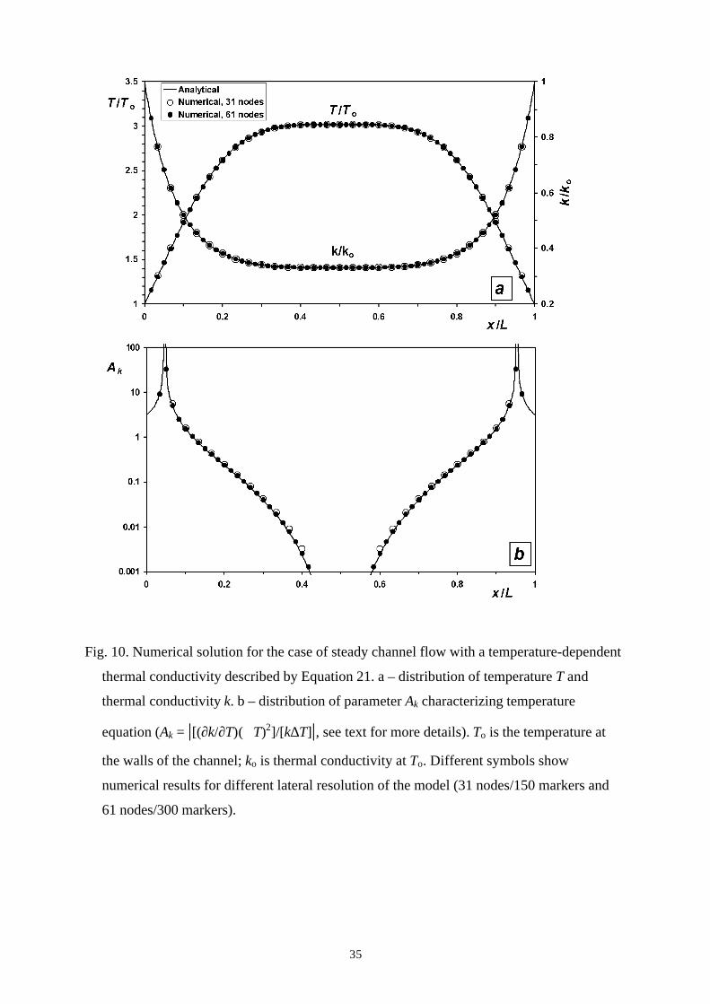
Figure 10 compares numerical and analytical results and shows strong (several orders of
magnitude) variations (Fig 10b) in parameter Ak in marginal zones of strong temperature
gradient (Fig 10a) resulted from significant shear heating. In this test a conductivity variation
of a factor of 3 across the channel is obtained (Fig. 10a). The maximum value of Ak exceed
102 (actually, goes to infinity due to the change in the sign of ∂2T/∂x2) close to the walls where
heat transport is mainly defined by the variations in thermal conductivity (Fig 10a). Figure 10
demonstrates the high accuracy of numerical solution, suggesting that adopted conservative
FD scheme correctly treats the heat transport in case of strong variations in thermal
conductivity.
3.8. Thermal convection with a large viscosity contrast and constant thermal conductivity
Thermal convection with a large viscosity contrasts from temperature dependent viscosity
is regarded as a challenging problem (Moresi and Solomatov, 1995). We have conducted tests
to check the efficacy of our numerical scheme in coping ably with the temperature and
momentum equations for convection with strong variations in temperature dependent
viscosity. First, we study steady-state convection with a strong temperature-dependent
viscosity in a square box of length L for a moderate irregularly-spaced lateral grid resolution
(43x43 nodes, 63,504 markers). A factor of two compression in the FD grid has been applied
to both the vertical and horizontal thermal boundary layers surrounding the box. The
boundary conditions correspond to free-slip along all boundaries, a specified temperature on
the top (T0) and at the bottom (T1) and ∂T/∂x=0 at the walls. Variable temperature-dependent
viscosity, according to the Frank-Kamnetzky approximation (e.g. Moresi and Solomatov,
1995; Albers, 2000), is used
η = η0exp[-ln(η0/η1)×(T-To)/(T1-To)], (25)
where η0 and η1 are maximal and minimal values of viscosity, the defining given η0/η1
Benchmark results are shown in Figure 11. Comparison (Fig. 11, values in brackets) of our
results with those of Albers (2000) shows a good accuracy for large (103-108) viscosity

19
contrast variations. Figure 12 compares the marker structure obtained without (Fig. 12 a) and
with (Fig 12 b) numerical diffusion for the selected area of the model shown in Figure 11b.
We can see that the introduction of numerical diffusion with d=1 (see Equation 12) prevent
the numerical oscillations of the temperature field associated with the markers in case of
strong chaotic mixing. This diffusion, however, does not notably affect the numerical solution
of temperature equation (see also Fig. 7 and 9).
The numerical simulations shown in Figures 11 and 12 do not account for the effects of
both shear and adiabatic heating to provide comparison with other authors who employed
only the Boussinesq approximation (e.g. Albers, 2000; Moresi and Solomatov, 1995).
However, these non-Boussinesq effects in the energetics can be very significant for modeling
of mantle convection problems (Yuen et al., 2000a). Figure 13a shows the temperature field
resulting from the influence of adiabatic and shear heating on the thermal convection model
shown in Figure 11b for the same moderate regularly spaced lateral grid resolution (43x43
nodes, 63,504 markers). The changes in the temperature field at characteristic values of the
box size (L = 423 km), pressure changes (0-12 GPa) and dissipation number (D = 0.12, where
D = αgL/Cp) are quite significant (8-12%, Fig. 13b). These changes are mainly resulted from
adiabatic heating and cooling (Fig 13 c). The effects of shear heating appeared to be one order
of magnitude smaller (Fig. 13 d).
3.9. Thermal convection with temperature dependent thermal conductivity and viscosity
These calculations are conducted to study 2-D spatial distribution of parameter Ak (see
Eq. 23) characterizing the nature of the heat transport process in case of temperature
dependent thermal conductivity for the moderate regularly spaced lateral grid resolution
(43x43 nodes, 63504 markers). This ratio measures the degree of nonlinearity of heat transfer
from variable thermal conductivity and indicates the local nature of the partial differential
equation involving the temperature. The model setup is the same as in section 3.8 and the
variable thermal conductivity is defined by the following equation applicable for the
ultramafic rocks of the upper Earth's mantle accounting for the phonon-dependence of the
thermal conductivity (Hofmeister, 1999; Clauser and Huenges, 1995)
k = 0.73 + 1293/(T +77). (26)
According to this equation (eqn.26) the thermal conductivity contrast for studied upper
mantle convection type models is k0/k1=2.6, where k0 and k1 are thermal conductivity in the
top and at the bottom of the model, respectively. Shear and adiabatic heating effects are also
taken into account in this extended-Boussinesq model. Figure 14 demonstrate temperature and
Ak structures of these models. Regions of high Ak=100-102 values, which indicate a strong

20
departure from the parabolic nature of the heat equation, are found in the upper portion of all
studied models (Fig. 14b, d, f) characterizing zones of strong vertical gradients in temperature
(Fig. 14a, c, e). Therefore, local changes in the parabolic character of temperature equation to
a non-linear hyperbolic-like partial differential equation due to the variable thermal
conductivity are relevant for the mantle convection models. Obviously, the correctness of
numerical solution in the high Ak regions crucially depends on conservation nature of finite-
difference formulation of the temperature equation. Another interesting feature of the Ak maps
is the capture of the great details in the temperature advection pattern, which shows up much
clearer than the temperature maps. This property can be exploited for visualization purposes
for studying strongly time-dependent mantle convection with variable thermal conductivity.
4. Discussion and Conclusions
In this paper we have described a recently constructed numerical code, which is based on
active or passive markers within the framework of a conservatively based finite-difference
code (I2VIS) written in the C-language. There are several new features of this code worth
emphasizing here. They include the following new capabilities with the following features:
(1.) The code can conserve stresses with strong variations of viscosity;
(2.) It can conserve heat-fluxes in time-dependent problems with sharply varying thermal
conductivity, temperature gradients and shear heating;
(3.) It can conserve scalar fields, such as temperature field, density, chemical
composition, and viscosity;
(4.) It can handle non-uniform FD grid with different stretching and compression factors.
These features are needed because of the increase in complexity in the physics of convection
and other modeling problems in geothermal-mechanics. For example, we have delineated the
regions in which the nonlinear nature of the variable conductivity in heat-transfer problem is
most obviously manifested (see Figs. 10 and 14). Previous codes can handle some of these
nonlinear aspects, but not all of them. For example, this is one of the first code to use markers
as a variant of a characteristics based method (Malevsky and Yuen, 1991) for solving the
temperature equation. De Smet et al. (1999) employed a variant of this characteristic method
for compositional field in melting dynamics. We have also used the direct matrix inversion
technique for solving both the momentum and temperature equations in 2-D, thus obtaining
more stable and higher accuracy solutions. This is made possible because of the increased
memory now available on shared-memory parallel computer architecture. Solving directly a
matrix associated with a 1000x1000 grid points, which amounts to around 100 Gbytes, is
feasible on a single node of a shared-memory machine today. In the case of the temperature
21
equation the implicit method allows for a much larger timestep than the commonly used
explicit timestepping. Implicit methods are more desirable because of the nonlinearities
present in both the variable thermal conductivity and viscous heating terms, which are
normally not included in many convection studies with the Boussinesq approximation (e.g.
Solomatov and Moresi, 1997; Trompert and Hansen, 1996; Albers, 2000). We would like to
stress the ease of the code implementation of the finite difference method combined with the
marker techniques. This allows one to implement other routines, such as involving kinetics in
phase transitions (Daessler and Yuen, 1996) or in grain-size dependent rheology (e.g.
Kameyama et al., 1997), where ordinary differential equations for the kinetics are solved at
each grid point.
The same marker technique can also be applied for advecting other scalar fields, such as
composition and also vector and tensor quantities, which would have direct applications in
thermal-chemical convection (Hansen and Yuen, 2000), the geodynamo (Glatzmaier, 2002)
and viscoelastic stress-transfer (Melini et al., 2002) problems. By using a rotating Lagrangian
frame of reference one can also solve efficiently the momentum equation in the dynamo
problem with extremely large number markers in excess of 1010, which are feasible in shared-
memory architecture. This may help to resolve better the Ekman boundary layer (e.g.
Desjardins et al., 2001). The work set out here lays the foundation for future in these
aforementioned areas.
Acknowledgements
This work was supported by RFBR grant # 00-05-64939, by an Alexander von Humboldt
Foundation Research Fellowship to T.V. Gerya, and by the Sonderforschungsbereich 526 at
Ruhr-University, funded by the Deutsche Forschungsgemeinschaft. Yuri Podladchikov and
Shalva Amiranashvili are thanked for discussions and comments. Support of this research has
come from the geophysics program of the National Science Foundation and the complex
fluids program of the Department of Energy.
References
Albers, M., 2000. A local mesh refinement multigrid method for 3-d convection problems
with strongly variable viscosity. J. Computational Phys. 160, 126–150.
22
Balmforth, N.G., Provenzale, A. (Eds.), 2001. Geomorphological Fluid Mechanics. Springer
Verlag, Berlin, 578 pp.
Barenblatt, G.I., 1996. Scaling, Self-Similarity, and Intermediate Asymptotics, Cambridge
Univ. Press, Cambridge, 386 pp.
Batchelor, G.K., 1967. An Introduction to Fluid Dynamics. Cambridge University Press, New
York, 615 pp.
Clauser, C., Huenges, E., 1995. Thermal conductivity of rocks and minerals. In: Ahrens, T.J.
(Ed.), Rock Physics and Phase Relations. AGU Reference Shelf 3, AGU, Washington
D.C., 105-126.
Christensen, U.R, and Yuen, D.A., 1984. The interaction of a subducting lithospheric slab
with a chemical or phase boundary. J. Geophys. Res. 89, 4389-4402.
Christensen, U.R., Yuen, D.A., 1985. Layered convection induced by phase transitions. J.
Geophys. Res. 90, 10291-10300.
Daessler, R., Yuen, D.A., 1996. The metastable wedge in fast subducting slabs: constraints
from thermokinetic coupling. Earth Planet. Sci. Lett. 137, 109-118.
Davies, J.H., Stevenson, D.J., 1992. Physical model of source region of subduction zone
volcanics. J. Geophys. Res. 97, 2037–2070.
Desjardins, B., Dormy, E., Grenier, E., 2001. Instability of Ekman-Hartmann boundary layers,
with application to the fluid flow nearthe core/mantle boundary. Phys. Earth Planet. Inter.
123, 15-26.
De Smet, J. H., van den Berg, A.P., Vlaar, N.J., Yuen, D.A., 2000. A characteristics-based
method for solving the transport equation and its application to the process of mantle
differentiation and continental root growth. Geophys. J. Int. 140, 651-659.
Dubuffet, F., Yuen, D.A., 2000. A thick pipe-like heat-transfer mechanism in the mantle:
nonlinear coupling between 3-D convection and variable thermal conductivity. Geophys.
Res. Lett. 27, 17-20.
Dubuffet, F., Yuen, D.A., Yanagawa, T., 2000. Feedback effects of variable thermal
conductivity on the cold downwellings in high Rayleigh number convection. Geophys.
Res. Lett. 27, 2981-2984.
Dubuffet, F., Yuen, D.A., Rainey, E.S.G., 2002. Controlling thermal chaos in the mantle by
positive feedback from radiative thermal conductivity. Nonlinear Proc. Geoph. 9, 311-323.
Fornberg, B., 1995. A Practical Guide to Pseudospectral Methods. Cambridge Univ. Press,
231 pp.

23
Fountaine, F., Rabinowicz, M., Boulegue, J., 2001. Permeability changes due to mineral
diagenesis in fractured crust: Implications for hydrothermal circulation at mid ocean
ridges. Earth Planet. Sci. Lett. 184, 407-425.
Gerya, T.V., Perchuk, L.L., van Reenen, D.D., Smit, C.A., 2000. Two-dimensional numerical
modeling of pressure-temperature-time paths for the exhumation of some granulite facies
terrains in the Precambrian. J. Geodynamics, 30, 17-35.
Gerya, T.V., Maresch, W.V., Willner, A.P., Van Reenen, D.D., Smit, C.A., 2001. Inherent
gravitational instability of thickened continental crust with regionally developed low- to
medium-pressure granulite facies metamorphism. Earth Planet. Sci. Lett., 190, 221-235.
Gerya, T.V., Perchuk, L.L., Maresch, W.V., Willner, A.P., Van Reenen, D.D., Smit, C.A.,
2002. Thermal regime and gravitational instability of multi-layered continental crust:
implications for the buoyant exhumation of high-grade metamorphic rocks. European J.
Miner. 14, 687-699.
Glatzmaier, G.A., 2002. Geodynamo simulations. How realistic are they? Annu. Rev. Earth
Planet. Sci. 30, 237-257.
Hansen, U., Yuen, D.A., 2000. Extended-Boussinesq Thermal-Chemical Convection with
moving heat sources and variable viscosity. Earth Planet. Sci. Lett. 176, 401-411.
Hockney, R.W., Eastwood, J.W., 1981. Computer Simulations Using Particles, Mc Graw-
Hill, Inc., 1981.
Hofmeister, A.M., 1999. Mantle values of thermal conductivity and the geotherm from
phonon lifetimes. Science, 283, 1699-1706.
Kameyama, M., Yuen, D.A., and Fujimoto, H., 1997. The interaction of viscous heating with
grain-size dependent rheology in the formation of localized slip zones. Geophys. Res. Lett.
24, 2523-2526.
Kameyama, M., Yuen, D.A., Karato, S., 1999. Thermal-mechanical effects of low-
temperature plasticity (the Peierls mechanism) on the deformation of a viscoelastic shear
zone, Earth Planet. Sci. 168, 159-172.
Kameyama, M., Kaneda, Y., 2002. Thermal-mechanical coupling in shear deformation of
viscoelastic material as a model of frictional constitutive relations. Pure Appl. Geophys.
159, 2011-2028.
Karato, S., 1997. Phase transformation and rheological properties of mantle minerals. In:
Crossley, D., Soward, A.M. (Eds), Earth's Deep Interior. Gordon and Breach, New York,
223-272.
Kincaid, C., Silver, P., 1996. The role of viscous dissipation in the orogenic process. Earth
Planet. Sci. Lett. 142, 271-288.

24
Lenardic, A., Kaula, W.M., 1993. A numerical treatment of geodynamic viscous flow
problems involving the advection of material interfaces. J. Geophys. Res. 98, 8243-8260.
Malevsky, A.V., Yuen, D.A., 1991. Characteristics-based methods applied to infinite Prandtl
number thermal convection in the hard turbulent regime. Phys. Fluids A 3, 2105-2115.
Malevsky, A.V., Yuen, D.A., 1992. Strongly chaotic non-Newtonian mantle convection.
Geophys. Astro. Fluid Dyn. 65, 149-171.
Melini, D., Cassarotti, E., Piersanti, A., Boschi, E., 2002. New insights on long distance fault
interaction. Earth Planet. Sci. Lett. 204, 363-372.
Moresi, L.N., Solomatov, V.S., 1995. Numerical investigation of 2D convection with
extremely large viscosity variations. Phys. Fluids 7, 2154 –2162.
Oran, E.S., Boris, J.P., 1987. Numerical Simulation of Reactive Flow. Elsevier, New York,
601 pp.
Patankar, S.V., 1980. Numerical Heat Transfer and Fluid Flow, Mc Graw-Hill, New York.
Ramberg, H., 1981. Gravity, Deformation and Geological Application. Academic Press,
London, 452 pp.
Ranalli, G., 1995. Rheology of the Earth, 2nd ed. Chapman and Hall, London, 413 pp.
Regenauer-Lieb, K., Yuen, D.A., Branlund, J., 2001. The initiation of subduction: critically
by addition of water? Science 294, 578-580.
Richard, G., Monnereau, M., Ingrin, J., 2002. Is the transition zone an empty water reservoir?
Inferences from numerical model of mantle dynamics. Earth Planet. Sci. Lett. (in press).
Riedel, M.R., Karato, S., 1997. Grain-size evolution in subducted oceanic lithosphere
associated with the olivine-spinel transformation and its effects on rheology. Earth Planet.
Sci. Lett. 148, 27-43.
Schatz, J.F., Simmons, G., 1972. Thermal conductivity of earth materials at high
temperatures. J. Geophys. Res. 77, 6966-6983.
Schott, B., Schmeling, H., 1998. Delamination and detachment of a lithospheric root.
Tectonophys. 296, 225-247.
Smolarkiewicz, P.K., Margolin, L.G. 1998. MPDATA: A finite-difference solver for
geophysical flows. J. Comput. Phys. 140, 459-480.
Solomatov, V.S., Moresi, L.-N., 1997. Three regimes of mantle convection with non-
Newtonian viscosity and stagnant lid convection on the terrestrial planets. Geophys. Res.
Lett. 24, 1907-1910.
Tackley, P.J., 1996. Effects of strongly variable viscosity on three-dimensional compressible
convection in planetary mantles. J. Geophys. Res. 101, 3311-3332.
25
Tikhonov, A.N., Samarsky, A.A., 1972. Equations of Math Physics. Nauka, Moscow (in
Russian).
Trompert, R.A., Hansen, U., 1996. The application of a finite-volume multigrid method to
three-dimensional flow problems in a highly viscous fluid with variable viscosity.
Geophys. Astrophys. Fluid Dyn. 83, 261-291.
Van den Berg, A.P., Yuen, D.A., Steinbach, V., 2001. The effects of variable thermal
conductivity on mantle heat transfer. Geophys. Res. Lett. 28, 575-578.
Virieux, J., 1986. P-SV wave propagation in heterogeneous media: Velocity-stress finite-
difference method. Geophysics 51, 889-901.
Weinberg, R.B., Schmeling, H., 1992. Polydiapirs: multiwavelength gravity structures. J.
Structural Geol. 14, 425-436.
Wesseling, P., 1992. An Introduction to Multigrid Methods. John Wiley and Sons, 1992.
Woods, A.W., 1999. Liquid and vapor flow in superheated rock. Annu. Rev. Fluid Mech. 31,
171-200.
Yuen, D.A., Balachandar, S., Hansen, U., 2000a. Modeling mantle convection: A significant
challenge in geophysical fluid dynamics. In: Fox, P.A., Kerr, R.M. (Eds.) Geophysical and
Astrophysical Convection. Gordon and Breach Sci. Publishers, 257-293.
Yuen, D.A., Vincent, A.P., Bergeron, S.Y., Dubuffet, F., Ten, A.A, Steinbach, V.C., Starin,
L., 2000b. Crossing of scales and non-linearities in geophysical processes. In: Boschi, E.,
Ekstrom, G., Morelli, A. (Eds.) Problems for the New Millennium. Editrice Compositori,
Bologna, Italy, 403-463.

26
Fig. 1. Schematic representation of non-regular rectangular staggered Eulerian grid used for
numerical solution of equations (1)-(4). gx and gz are components of gravitational acceleration
in the x-z coordinate frame. Different symbols correspond to the nodal points for different
scalar properties, vectors and tensors. i, i+½, etc. and j, j+½, etc. indexes represent the
staggered grid and denote, respectively, the horizontal and vertical positions of four different
types of nodal points. Many variables (vx, vz, σxx, σxz, σzz, εxx, εxz, εzz, P, T, η, ρ, k, Cp, etc.), up
to around 25 at grid point, are part of the voluminous output in this code.
27
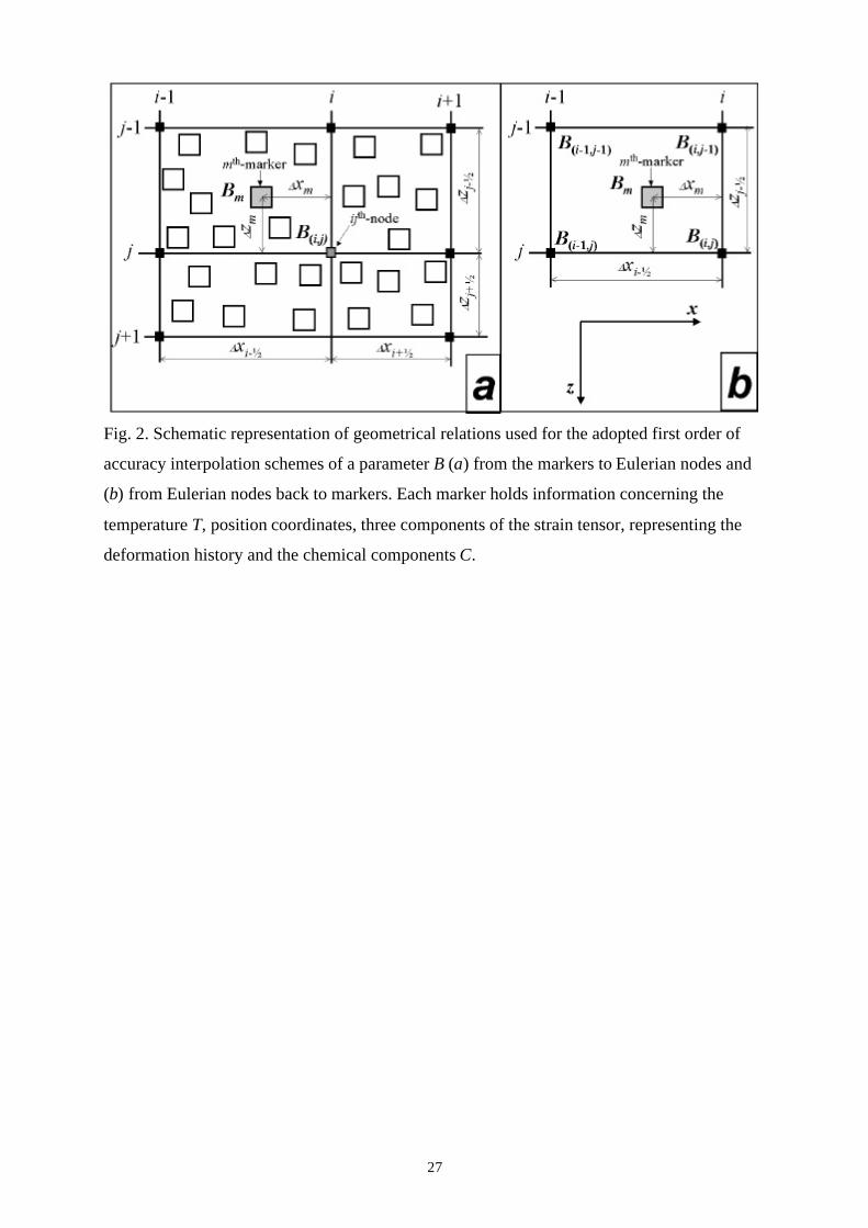
Fig. 2. Schematic representation of geometrical relations used for the adopted first order of
accuracy interpolation schemes of a parameter B (a) from the markers to Eulerian nodes and
(b) from Eulerian nodes back to markers. Each marker holds information concerning the
temperature T, position coordinates, three components of the strain tensor, representing the
deformation history and the chemical components C.

28
Fig. 3. Flow chart representing the adopted computational strategy used in the programming
of the computer code I2VIS. Panel for step 6 shows the scheme for interpolating the
calculated temperature changes from the Eulerian grid to the moving markers.

29
Fig. 4. Numerical solutions for the case of the Rayleigh-Taylor instability of a two-layer
cross-section in the gravity field. Numerical and analytical solutions are compared for the
factor of growth K at different viscosity contrast between the upper (η1) and the lower (η2)
layer and different wave number (a=2πh/λ, where h is layer thickness and λ is
wavelength) and amplitude (y) of initial sinusoidal disturbance at the layer boundary. Grid
resolution of the model: 32x31 nodes, 23250 markers.

30
Fig. 5. Results of numerical experiments for the sinking of rectangular block at different
viscosity contrast between the block and the surrounding soft medium (see text for
discussion). Boundary conditions: free slip at all boundaries. Black and white dots
represent positions of markers for the block and the medium, respectively. Grid resolution
of the model is 51x51 nodes, 22500 markers.

31
Fig. 6. The results of test of numerical solution for the case of power-law flow in the channel
of width L. vz0 is the velocity in the center of the channel, η0 is the viscosity at the walls
(see Eq. 17). Different symbols show the numerical results for the different lateral
resolution of the model (31 nodes/150 markers and 16 nodes/75 markers).

32
Fig. 7. The result of test of numerical solution for non-steady temperature changes within the
Newtonian channel flow. Different symbols show the solutions calculated with (d=1) and
without (d=0) numerical diffusion (see equation 12). t0 = ρCpL2/k is characteristic
timescale, ∆T0 = 5vz0(∂To/∂z)ρCpL2/(48k) is maximal temperature change in the center of
the channel corresponding to the final steady temperature profile. Lateral resolution of the
model: 31 nodes, 150 markers.

33
Fig. 8. Results of test of a numerical solution for the case of steady Couette flow with a
temperature dependent viscosity (see equation 20) and shear heating. Θ = E(T-To)/[R(To)2]
is non dimensional temperature change; Br = (σxzL/To)2×exp(-E/RTo)/(RkCp) is Brinkman
number. a – reproducing of analytical relations (Turcotte and Schubert, 1982) of maximal
temperature change within the flow Θ1 and Brinkman number Br, b – comparison of
analytical and numerical solutions for the distribution of temperature across the flow at
different Brinkman number. Lateral resolution of the model: 32 nodes, 310 markers.

34
Fig. 9. The results of test of numerical solution for the solid body rotation of a square
temperature wave. Figure shows the horizontal profiles across temperature wave at
different time t after given number of revolutions. ∆T0 and ∆T are initial and calculated
amplitude of temperature waive, respectively; t0 = ρCpL2/k is characteristic timescale; d is
numerical diffusion parameter (see Eq. 12). Resolution of the model: 31x31 nodes,
150x150 markers.
35
Fig. 10. Numerical solution for the case of steady channel flow with a temperature-dependent
thermal conductivity described by Equation 21. a – distribution of temperature T and
thermal conductivity k. b – distribution of parameter Ak characterizing temperature
equation (Ak = |[(∂k/∂T)(∇T)2]/[k∆T]|, see text for more details). To is the temperature at
the walls of the channel; ko is thermal conductivity at To. Different symbols show
numerical results for different lateral resolution of the model (31 nodes/150 markers and
61 nodes/300 markers).

36
Fig. 11. Results of tests for stationary thermal convection in square box with temperature
dependent viscosity (equation 25) and constant thermal conductivity k. Ra1 = αgρ(T1-
T0)/(kη1) is the Rayleigh number, Nu = 1/L∫∂T/∂z dx is the calculated value of Nusselt
number (in brackets are the values interpolated from Albers (2000) for given grid
resolution). The effects of adiabatic and shear heat production are neglected. a and b
demonstrate numerical results for varying viscosity contrasts. Rectangle in b show area
zoomed in Figure 12. Model resolution: 43x43 nodes, 63504 markers.

37
Fig. 12. Marker structure for zoomed-in area of the numerical model shown in Figure 11b.
Different colors of markers correspond to different value of temperature ascribed to the
markers. a and b show the results calculated without (d=0) and with (d=1) numerical
diffusion (see Equation 12), respectively.

38
Fig. 13. Effects of shear and adiabatic heating on thermal convection. Model design and
resolution correspond to Figure 11b, box size - L = 423 km, pressure change from the top
to the bottom of the model - ∆P = 12 GPa, dissipation number - D = 0.12 (D = αgL/Cp). a
– temperature structure of the model. b – temperature differences ∆T compared to the
model neglecting shear and adiabatic heating (Fig 11b). c and d – thermal effects of
adiabatic (Ha) and shear (Hs) heat production (see equation 4), respectively. The value
H0=k(T1-T0)/L2 is used for normalization.
39
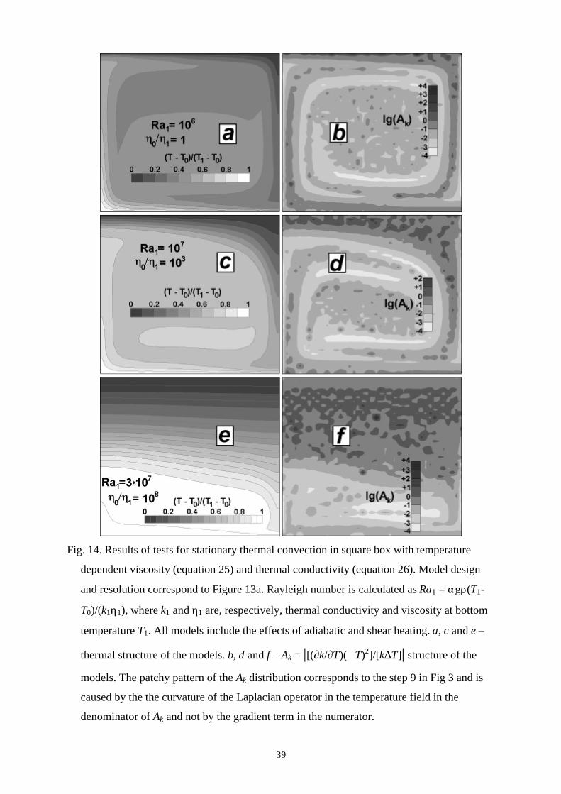
Fig. 14. Results of tests for stationary thermal convection in square box with temperature
dependent viscosity (equation 25) and thermal conductivity (equation 26). Model design
and resolution correspond to Figure 13a. Rayleigh number is calculated as Ra1 = αgρ(T1-
T0)/(k1η1), where k1 and η1 are, respectively, thermal conductivity and viscosity at bottom
temperature T1. All models include the effects of adiabatic and shear heating. a, c and e –
thermal structure of the models. b, d and f – Ak = |[(∂k/∂T)(∇T)2]/[k∆T]| structure of the
models. The patchy pattern of the Ak distribution corresponds to the step 9 in Fig 3 and is
caused by the the curvature of the Laplacian operator in the temperature field in the
denominator of Ak and not by the gradient term in the numerator.