characteristics of uncertainty indices in the macroeconomy

Characteristics of Uncertainty Indices in the Macroeconomy

Takeshi Shinohara* [email protected]

Tatsushi Okuda** [email protected]

Jouchi Nakajima* [email protected]

No.20-E-6 October 2020

Bank of Japan 2-1-1 Nihonbashi-Hongokucho, Chuo-ku, Tokyo 103-0021, Japan

* Research and Statistics Department ** Research and Statistics Department (currently at the Financial System and Bank

Examination Department)

Papers in the Bank of Japan Working Paper Series are circulated in order to stimulate discussion and comments. Views expressed are those of authors and do not necessarily reflect those of the Bank. If you have any comment or question on the working paper series, please contact each author. When making a copy or reproduction of the content for commercial purposes, please contact the Public Relations Department ([email protected]) at the Bank in advance to request permission. When making a copy or reproduction, the source, Bank of Japan Working Paper Series, should explicitly be credited.

Bank of Japan Working Paper Series

Characteristics of Uncertainty Indices in the Macroeconomy*

Takeshi Shinohara† Tatsushi Okuda‡ Jouchi Nakajima§

October 2020

Abstract

In macroeconomics, a variety of uncertainty indices have been proposed to

quantitatively assess developments in uncertainty of the macroeconomy. This paper

empirically investigates the time series properties of major uncertainty indices and their

relationship with macroeconomic variables, using U.S. and Japanese data. Specifically,

we analyze: (i) the Macroeconomic Uncertainty Index, (ii) the Economic Surprise Index,

(iii) the Volatility Index, and (iv) the Economic Policy Uncertainty (EPU) Index. The

empirical analysis for the U.S. shows that, except for EPU, these indices share similar

developments and can significantly explain the business cycle fluctuations of investment,

durable consumption, and the lending attitude of banks. In contrast, the empirical

analysis for Japan reveals significant heterogeneities in the characteristics of the indices.

The Macroeconomic Uncertainty Index (i), responds to various events and shows a

significant relationship with investment and durable consumption. On the contrary, the

Economic Surprise Index (ii), barely reacts to the events and exhibits limited

performance in explaining business cycles. The Volatility Index (iii), tends to rise when

the financial system is stressed, whereas the Economic Policy Uncertainty Index (iv), is

likely to respond to overseas events, and both of these indices can significantly explain

business cycle fluctuations of investment and the lending attitudes of banks.

JEL classification: E32, E52.

Key words: Uncertainty, Business cycle.

* The authors thank Kosuke Aoki, Ryo Jinnai, Seisaku Kameda, Kazushige Kamiyama, Takuji Kawamoto, Takashi Nagahata, Teppei Nagano, Koji Takahashi, Yoichi Ueno, Francesco Zanetti, and the staff at the Bank of Japan for their valuable comments. Any remaining errors are the sole responsibility of the authors. The views expressed in this paper are those of the authors and do not necessarily reflect the official views of the Bank of Japan. † Research and Statistics Department, Bank of Japan ([email protected]) ‡ Research and Statistics Department, Bank of Japan (currently, Financial System and Bank Examination

Department; [email protected]) § Research and Statistics Department, Bank of Japan ([email protected])

1

1. Introduction

An increase in uncertainty has macroeconomic consequences by yielding a temporary

slowdown in economic activities of households and firms. In recent years, we have

experienced various events that have elevated the uncertainty faced by economic agents in

the macroeconomy, such as the Global Financial Crisis (GFC) in 2008, the European debt

crisis around 2012, trade tension between the U.S. and China, and more recently, the spread

of COVID-19. These situations make it increasingly important to quantitatively assess the

degree of uncertainty and its implications on the macroeconomy.

Against this backdrop, a major body of studies has developed various indices to capture

developments in uncertainty, mainly for the U.S.1 For instance, Bloom (2009) analyzes the

“Volatility Index (VI)” as a proxy for the degree of uncertainty, and Jurado et al. (2015),

Rossi and Sekhposyan (2015), Scotti (2016), and Sekkel (2019) propose uncertainty indices

based on discrepancies between predicted values of economic indicators and their realized

values. Among them, Jurado et al. (2015) develop the “Macroeconomic Uncertainty Index

(MU)”, which is based on forecast errors in time series models for economic indicators.

Scotti (2016) proposes the “Economic Surprise Index (ES)”, which builds on the forecast

errors of professional forecasters. Baker et al. (2016) and Arbatli et al. (2017) develop the

“Economic Policy Uncertainty Index (EPU)”, based on the text of newspapers, which has

been practically and widely used as the index to monitor the uncertainty in real-time manner.

While various uncertainty indices have been proposed, there are only a few comparative

studies about the empirical properties of the uncertainty indices. In one of these, Meinen and

Röhe (2017) compare the empirical relationships between each of the uncertainty indices

and investment using Euro-area data, and conclude that the MU developed by Jurado et al.

(2015) explains the negative relationship between those two variables in the most robust

manner. To our best knowledge, there is no study comparing the characteristics of the

uncertainty indices and their relationship with the business cycle for the U.S and Japan.

To fill the gap, this paper provides comparisons of the characteristics of uncertainty

indices for the macroeconomy that have been proposed in the existing literature, and their

relationship with macroeconomic variables, using data for the U.S. and Japan. Specifically,

we focus on the four major indices mentioned above: (i) the MU, (ii) the ES, (iii) the VI, and

1 Bloom (2014) and Ferrara et al. (2017) provide surveys for the uncertainty indices. Economists at the Federal Reserve Board review various uncertainty indices, explaining how to create the indices and their characteristics (Cascaldi-Garcia et al., 2020).

2

(iv) the EPU.2 We analyze the time-series properties of the uncertainty indices and their

responses to past events. We then quantitatively assess the relationship between the indices

and macroeconomic variables using the VAR model. While most existing literature only

focuses on the link between the uncertainty indices and investment, this study

comprehensively explores the relationship of the indices with investment, durable

consumption, and financial variables. Because the MU for Japan has not been developed

anywhere, we compute it ourselves following Jurado et al. (2015).

We stress the advantage of comparing characteristics of the uncertainty indices by using

data for both the U.S. and Japan. Because the indices have mostly been proposed based on

U.S. data, the methods to compute each index could depend on the predictive power of the

indices for U.S. macroeconomic variables. However, the macroeconomic environment

differs between the U.S and Japan at times of significant historical events; in addition, the

degree of risk aversion and economic structure also differ. Therefore, this analysis could

uncover the characteristics of each index in macroeconomics and show how differently

economic agents react to changes in uncertainty in the U.S. and Japan, by investigating the

similarities and differences of the various uncertainty indices in these two countries.

There are two concepts for uncertainty: “risk” and “Knightian uncertainty” (or

“ambiguity”; Knight, 1921). The concept of risk captures the dispersion of the quantifiable

probabilistic distribution about the future values of macroeconomic variables. In contrast,

the concept of ambiguity corresponds to the degree of a lack of any quantifiable knowledge

about some possible occurrence of macroeconomic variables. While an increase in both

types of uncertainty deteriorates the macroeconomy, the channels and quantitative impacts

of each type can be different. As indicated by existing literature, the proposed uncertainty

indices do not distinguish between these two types of uncertainty (Bloom, 2014). In the VAR

analysis, the contributions of risk and ambiguity to changes in the uncertainty indices are

assumed to be constant at their historical averages. At the time of extreme events, the

influence of an increase in the uncertainty indices on the macroeconomy where the

contributions of risk and ambiguity are considered to be considerably different from the

historical average, such as during the spread of COVID-19, could be significantly different

from the result in the VAR analysis. Therefore, we have to bear this in mind when applying

the results of this paper to such extreme events.

The remainder of the paper is organized as follows. Section 2 introduces four

2 This paper only focuses on the uncertainty indices that are publicly available and updated to recent periods. We exclude, for instance, the uncertainty index based on disagreements among professional forecasts on the economic indicators (Lahiri and Sheng, 2010; Bachman et al., 2013).

3

uncertainty indices and compares their time-series properties. Section 3 quantitatively

assesses the relationship between the indices and the macroeconomic fluctuations, using the

VAR model. Finally, Section 4 concludes.

2. Macroeconomic Uncertainty Indices

The uncertainty indices in this paper are expected to capture what has been referred to as

“uncertainty” as a general term, but neither of them corresponds to the comprehensive

concept of “uncertainty” in economic models, and different indices capture different types

of uncertainty. The assumptions behind the method for quantifying “uncertainty” —an

abstract concept— in the economic models are also different across indices. This section

first describes the correspondence relation between each index and type of uncertainty in

macroeconomic theory, and then explains the methods used to create the indices. For the

sake of simplicity, in what follows, we consider uncertainty as being based on the concept

of “risk” as mentioned above.

2-1. Uncertainty in macroeconomic models

The standard economic theory defines the uncertainty for economic agent as the

unconditional expectations of the discrepancy between agents’ beliefs about decision-related

economic variables and the underlying actual values. The theory also predicts that the

economic agent ’s action (e.g., investment, consumption, and bank lending) in period

depends on the uncertainty of a variety of current and future ( 1 period) economic

variables. In addition, there are various channels through which uncertainty affects the agents’

decisions.

The concept of uncertainty for the economic agent is roughly divided into the

uncertainty of macroeconomic aggregate variables and the agent’s idiosyncratic variables,

as illustrated in the chart below. The uncertainty of macroeconomic variables includes not

only the uncertainty on variables of real economy, but also that of financial variables. The

uncertainty is caused by various factors including developments in the foreign economy,

energy prices, asset prices, banking sector development, and macroeconomic policies. In this

paper, we exclude measures for the uncertainty of economic agents’ idiosyncratic variables

from our analysis, which also have been proposed by existing studies.3

3 For example, several studies propose uncertainty measures for the economic agents’ idiosyncratic variables based on the heterogeneity of stock prices and TFP growths across individual firms (Bloom et al., 2007; Bloom, 2009; and Gilchrist et al., 2014).

4

Chart: Uncertainty in macroeconomic models and the scope of this study.

2-2. Construction of the uncertainty indices

To measure the uncertainty of the macroeconomy based on real data, an index must focus

on some of the possible causes for the uncertainty. As discussed above, the causes of such

uncertainty could be exogenous shocks (other than macroeconomic policies) on the real

economy and financial conditions, as well as shocks generated by macroeconomic policies.

Focusing on this point, the concept of each uncertainty index is summarized as follows (see

also the chart below).

(1) MU is based on forecast errors of predicted values (computed by simple econometric

models) on a variety of economic indicators including the indicators for financial

conditions. This implies that the index aims to simply but comprehensively capture the

uncertainty caused by various factors.

(2) ES is based on forecast errors of predicted values about economic indicators on the

real economy that are made by professional forecasters right before the release of the

indicators. This implies that the uncertainty arises when the macroeconomy deviates

from what economic agents forecast with almost all of the available information. The

index aims to capture the uncertainty of real economic activity rather than financial

conditions.

(3) VI is based on stock market participants’ expectations about the volatility of the stock

prices in the future. This implies that the index focuses on the uncertainty of the

financial conditions which investors face.

(4) EPU is based on newspaper coverage, capturing uncertainty about macroeconomic

policy available to the public through the media.

Uncertainty for economic agent

Uncertainty of macroeconomic

variables

Uncertainty of the agent ’s

idiosyncratic variables

+

Out of scope in this study

(1) Macroeconomic Uncertainty Index

(2) Economic Surprise Index

(3) Volatility Index

(4) Economic Policy Uncertainty Index

5

Chart: Concepts of the uncertainty indices.

We describe the method to calculate each uncertainty index as follows (see also

Appendix 1, for their interpretation using mathematical expression).

(1) Macroeconomic Uncertainty Index (MU)

Jurado et al. (2015) construct the MU for the U.S. by employing 132 monthly economic

indicators collected from seven categories, including data on production, employment, retail

sales, prices, and stock markets. Following Jurado et al. (2015), we create the MU for Japan.

We collect as many monthly economic indicators as possible; the resulting dataset consists

of 67 indicators from the same seven categories as the U.S. (see Appendix Figure 1 for the

list of indicators).

By applying principal component analysis for the indicators, their common factors are

extracted (12 factors for the U.S. and four factors for Japan).4 In addition, the first common

factor for the squares of the indicators is also extracted to capture a possible non-linearity in

4 Because the contribution of a fifth factor in Japan is quite small, we set the number of factors as four. Jurado et al. (2015) use 147 indicators for financial conditions in addition to 132 economic indicators in their principal component analysis. In constructing the Japan index, no additional indicator on financial conditions is used, because fluctuations of indicators on Japanese financial markets are small for long periods of time, unlike in the U.S.

Real economy Economic policy Financial condition

(1) Macroeconomic Uncertainty Index

(2) Economic Surprise Index

(3) Volatility Index

(4) Economic Policy Uncertainty Index

Forecast errors of simple econometric models

Forecast errors of professional forecasters

Stock market participants’ implied volatility of future stock prices

Newspaper coverage frequency

Main coverage for constructing the index

6

the economic agents’ forecasting for macroeconomic variables.

We estimate the linear time series model that includes common factors and the own lags

of economic indicators as explanatory variables, and obtain the one-month-ahead forecast

for each economic variable. Then, we estimate the stochastic volatility model for the forecast

errors between the ex-ante forecast and the realized value to obtain the time-varying variance

as the estimate of uncertainty for each economic indicator. Finally, the MU is composed by

simply averaging the variances across all economic indicators and calculating its square root.

The time-series data of the MU for the U.S. is obtained from the website, https://

www.sydneyludvigson.com/macro-and-financial-uncertainty-indexes. The MU for Japan is

created in this paper. The series is available from 1960/Q3 for the U.S. and 1979/Q2 for

Japan.

(2) Economic Surprise Index (ES)

Scotti (2016) constructs the ES based on the forecast errors of professional forecasts of

economic indicators. Specifically, we use six indicators (GDP, industrial production,

employment, retail sales, ISM manufacturers index, and personal income) in the U.S., and

five (GDP, industrial production, unemployment rate, retail sales, business conditions DI in

the Tankan survey) in Japan. We use the median of predicted values that are made by

professional forecasters in Bloomberg, immediately before the release of the indicators.

We calculate a square root of weighted averages of the squared forecast errors for the

indicators. To take the average, we use weights obtained from dynamic factors models fit to

the indicators. This implies that the more the economic indicator contributes to the common

factors, the larger the weight is. It is noted that the number of economic indicators used for

the ES is quite limited (only five or six), compared to those used for the MU (over 100). In

addition, the ES does not include financial variables in its dataset.

The time-series data of the ES for the U.S. and Japan is obtained from the website,

https://sites.google.com/site/chiarascottifrb/research. The series is available since 2003/Q2

for both the U.S and Japan.

(3) Volatility Index (VI)

The VI is the implied volatility of the stock indices in 30 days, calculated from the prices of

stock options. It is often referred to as the “fear gauge.” The VI could be interpreted as the

expectations of financial market participants regarding their own forecast errors on future

7

stock prices, if we assume that the stock prices follow random-walk process.5 This paper

uses the VIX calculated by Chicago Board of Option Exchange (CBOE) for U.S., and the

Nikkei Volatility index (Nikkei VI) for Japan. Note that Nikkei VI is the implied volatility

of the Nikkei Stock Average in 30 days.

The time-series data of the VIX is obtained from the St. Louis Fed FRED for the U.S.,

and Nikkei Inc. for Japan. The series is available from 1990/Q1 for the U.S., and from

2001/Q1 for Japan.

(4) Economic Policy Uncertainty Index (EPU)

Baker et al. (2016) and Arbatli et al. (2017) construct the EPU based on the newspaper

coverage frequency to quantify the uncertainty of the economic policies. The number of

newspapers used for the EPU is 10 in the U.S. and four in Japan.6

We use articles in each newspaper that include at least one word listed in all three

categories: “economy”, “policy”, and “uncertainty”, and count them for each month. We

then divide the number of articles by the total number of articles in the same newspaper and

in the month, to compute the “relative coverage frequency.” Finally, the EPU is calculated

by taking simple averages of the relative coverage frequency. In addition to the total index

for all the economic policies, sub-series of the EPU for individual policy such as fiscal policy

and monetary policy are created. These sub-series EPUs are generated by counting the

number of the articles that include the word related to each policy in addition to the three

categories above.7

The time-series data of the EPU for the U.S. and Japan are obtained from the website,

https://www.policyuncertainty.com/. The series is available from 1985/Q1 for the U.S., and

1987/Q1 for Japan.

5 It is known that the VI could fluctuate due to idiosyncratic factors in the stock market because the VI is calculated based on the market participants’ expectations on stock prices and thus it mainly captures the uncertainty of the stock market rather than the uncertainty of the macroeconomy. For example, Bekaert et al. (2013) point out that the VI responds not only to changes in uncertainty but also to changes in risk premiums along with the changes in the market participants’ risk aversion. 6 The index for the U.S. includes USA Today, Miami Herald, Chicago Tribune, Washington Post, Los Angeles Times, Boston Globe, San Francisco Chronicle, Dallas Morning News, Houston Chronicle, and Wall Street Journal; for Japan, Asahi, Nikkei, Mainichi, and Yomiuri. 7 For the index in the U.S., media coverage is expanded to regional newspapers when the subseries for individual policy is created.

8

2-3. Developments in the uncertainty indices

This subsection describes how the uncertainty indices have responded to economic events

since the 1990s. To facilitate comparison between them, we standardize the indices to zero

mean and unit standard deviation using the time series up to end-2019. We transform the

monthly indices to quarterly series by taking simple averages of the monthly indices, because

the monthly indices are quite volatile and the economic indicators used in the following

analysis are quarterly.

Figure 1 shows the developments in the uncertainty indices for the U.S. It demonstrates

that almost all the indices sharply increased during the GFC. The EPU exhibits different

trajectories from other indices, increasing not only during the GFC, but also the Iraq War in

the early 2000s and the debt ceiling dispute in 2011. The MU, the VI, and the EPU, which

are available for recent periods, have risen sharply because of the spread of the COVID-19,

and in particular, the increases in the MU and the EPU are remarkable.8

The correlation coefficients between indices are reported in the table below. The

correlation coefficients of the MU, the ES, and the VI are around 0.6 and 0.7, while the EPU

has a significantly lower correlation with other indices with correlation coefficients from 0.1

to 0.4. This difference implies that the EPU responds to economic events differently to other

indices.

Table: Correlation coefficients between uncertainty indices for the U.S.

EPU VI ES

MU 0.23 0.65 0.69

ES 0.05 0.58

VI 0.37

Note: Estimated for data from the period available to 2019/Q4.

Figure 2 plots the developments of the uncertainty indices for Japan. Unlike those for

the U.S., the timing of the hikes differs among the indices. The characteristics for each index

are summarized as follows.

8 Baker et al. (2020) assess the influence of the spread of the COVID-19 on the U.S. economy using the macroeconomic model that takes into account the uncertainty in the stock market. Their estimates show that more than half of contraction in GDP would be attributable to increasing uncertainty. Ludvigson et al. (2020) show the amplification mechanism of the temporary contraction due to the spread of the COVID-19 would endogenously make the uncertainty higher, and the rise in the uncertainty would depress the economy for a long period. Leduc and Liu (2020) argue that the pandemic levers uncertainty up, which could lead to contraction and disinflation pressure in the U.S.

9

(1) The MU rose sharply during the GFC (2008-2009), the Great East Japan Earthquake in

March 2011, and the hikes in the consumption tax rate in April 1997 and April 2014.9

The MU has been recently at a historical high, in response to the spread of COVID-19.

(2) The ES responded only to the Great East Japan Earthquake, except for 2019. It should be

noted that the ES did not significantly rise during the GFC. It is probably because the

predicted values by professional forecasters, reported right before the release of the

domestic economic indicators, had already reflected the impact of the crisis on the

Japanese economy with information on U.S. economic indicators and Japanese trade

indicators that were released earlier.

(3) The VI increased only during the GFC, which is consistent with the idea that the VI

captures the uncertainty faced by participants in financial markets (particularly stock

markets). The MU and the ES responded to the Great East Japan Earthquake and to

increases in the consumption tax rate, though the VI did not respond to either of them.

(4) The EPU is unique in the sense that it responds to different economic events from other

indices and it rises quite frequently. In chronological order, the EPU clearly went up in

response to the domestic financial crisis from 1997 to 1998, the GFC, the Greek debt

crisis in 2010, the European debt crisis in 2011, and Brexit in 2016. The EPU is more

likely to respond to events originating overseas than the other indices.10 This reflects

that the EPU also rises when the domestic media cover policies from overseas. The EPU

rose to high levels from 2018 to the mid-2019 in response to the trade tension between

the U.S. and China, fell once in the second half of 2019, and then recently increased

significantly in response to the rapid increase in the number of articles in newspapers on

measures responding to the spread of COVID-19.

The below table shows that the correlation coefficients between the indices for Japan

are lower than those for the U.S., which is consistent with the observation that the indices

for Japan tend to respond to different economic events.

9 The rise in the MU around the tax rate hike could be attributable to the last-minute demand before the tax rate hike and a rebound from it. 10 Ito (2019) notes this characteristic of the EPU for Japan.

10

Table: Correlation coefficients between uncertainty indices for Japan.

EPU VI ES

MU 0.23 0.48 0.35

ES 0.13 0.04

VI 0.53

Note: Estimated for data from the period available to 2019/Q4.

3. The Uncertainty Indices and Macroeconomic Business Cycle

This section quantitatively assesses the relationship between the uncertainty indices and

macroeconomic variables. Specifically, we investigate whether the rises in the uncertainty

indices incrementally exacerbate investment, durable consumption and bank lending attitude

relative to the average pattern of business cycle, as is consistent with the theory.

3-1. Economic theory on uncertainty and the macroeconomic business cycle

“The real option channel” in firms’ investment decisions and “the precautionary saving

channel” are widely discussed as mechanisms by which rises in uncertainty depress the

economy.11

The real option channel was proposed by Bernanke (1983), Brennan and Schwartz

(1985), McDonald and Siegel (1986), and Dixit and Pindyck (1994). It shows that firms are

more likely to choose a wait-and-see strategy for irreversible decision-making, including

making investments or hiring new staff. For example, if a firm has an option to postpone its

decision on an investment project until the resolution of uncertainty becomes clear, the real-

option value (the value of putting off its decision) for the firm would increase as the degree

of uncertainty rises, and the firm is more likely to choose to postpone its decision. Guiso and

Parigi (1999) argue that uncertainty affects firms’ decisions more as investment projects are

more irreversible.

The precautionary saving channel was proposed by Leland (1968) and Kimball (1990).

11 Some studies argue that rises in uncertainty could stimulate the economy (e.g., Bar-IIan and Strange, 1996). Among others, the growth option channel is widely known. In the theory, the firms’ losses from its investment are bounded above at the investment costs and firms’ returns are unbounded. Then, the risk-taking incentive for the firms could exceed the incentive to postpone their decision due to the increase in real-option value if the decision is relatively reversible, and the rises in the uncertainty eventually promote the investment. Other studies discuss the risk-loving nature of firms because they can hedge the risk for the investment projects (Oi, 1961; Hartman, 1972; Abel, 1983).

11

This mechanism functions so that households increase their saving in order to smooth their

inter-temporal consumption allocations if they perceive a rise in the uncertainty of their

future incomes (labor incomes and dividends). In particular, the precautionary saving

channel is expected to be more pronounced in expensive and luxury goods including durable

goods.

In addition, the financial frictions channel has also been a focus of economists’ attention.

The rise in uncertainty increases the default risk of borrowing firms and banks shift the

increased risk onto the lending rates. Then, these higher lending rates depress firms’

investment activities (Christiano et al. 2014; Arellano et al., 2019). Many studies indicate

that this channel played a crucial role in transmitting the rise in uncertainty into the economy

during the GFC (Stock and Watson, 2012; Gilchrist et al., 2014; Caldara et al., 2016;

Ludvigson et al., 2019).

In the following, we examine the empirical validity of these theoretical projections: the

negative relationship between the uncertainty index and macroeconomic variables.

Specifically, we investigate whether the fluctuations of the uncertainty indices can explain

the deviation of macroeconomic variables from their business cycles using VAR models.

3-2. Econometric methodology

We estimate eight-variable VAR models, which are canonical mid-scale models of the

macroeconomic variables with the uncertainty index added. Each VAR model includes one

of the macroeconomic variables that are expected to be affected by macroeconomic

uncertainty: (1) investment (Model I); (2) durable consumption (Model II); and (3) bank’s

lending attitude (Model III). We employ these VAR models with a relatively large number

of variables to control relationships between the variables that are not caused by uncertainty,

i.e., the business cycle fluctuations in normal times. If we do not control these fluctuations,

our estimates may be biased due to omitted variables. Because the macroeconomic

uncertainty indices are calculated with the economic indicators, the endogenous problem—

that uncertainty indices rise when large macroeconomic fluctuations occur—may be present.

Following previous studies on the uncertainty index and on VAR models for macroeconomic

variables (e.g., Christiano et al., 2005), the specifications of the VAR models are set as in the

tables below.

12

Table: Specifications of the VAR models.

(1) U.S.

Model I Model II Model III

Uncertainty index Uncertainty index Uncertainty index

Industrial production Industrial production Industrial production

Investment Durable consumption Stock price (S&P500)

Stock price (S&P500) Stock price (S&P500) Banks’ lending attitude

Nominal wage Nominal wage Nominal wage

PCE deflator PCE deflator PCE deflator

FF rate FF rate FF rate

M2 M2 M2

(2) Japan


Uncertainty index Uncertainty index Uncertainty index

Industrial production Industrial production Industrial production

Investment Durable consumption Stock price (TOPIX)

Stock price (TOPIX) Stock price (TOPIX) Banks’ lending attitude

Nominal wage Nominal wage Nominal wage

GDP deflator GDP deflator GDP deflator

Call rate Call rate Call rate

M2 M2 M2

Note 1: Uncertainty indices, FF rate, call rate, and banks’ lending attitude are all levels. All others are the logarithm of the levels. Data sources except for the uncertainty indices are listed in Appendix 2.

Note 2: Shocks are identified by Cholesky decomposition. The number of lags is two.

In the following analysis, we examine impulse responses of (1) investment, (2) durable

consumption, and (3) banks’ lending attitude to the one standard deviation shock on the

uncertainty index and test that the response is negative and statistically significant.12 We

12 To facilitate the comparison of the impulse responses, we reverse the sign of the indicator of banks’ lending attitude in the U.S., as the larger number implies an easier lending attitude.

13

identify the shock via Cholesky decomposition. While some previous studies report that

macroeconomic variables are inclined to rebound after contraction, we exclude such a case

of rebound from our assessment.

Note that as the initial available periods of the uncertainty indices are different, the

sample periods for the estimation of VAR models could be different. We estimate each VAR

model with all the available data as a main baseline analysis, and additionally estimate them

using the same sample period (from 2003/Q4 to 2019/Q2) to check the robustness of the

results (see Appendix 3).

3-3. Time-lagged correlation

As a preliminary analysis, we assess the correlation coefficients between the uncertainty

indices and economic indicators of investment, durable consumption, and the diffusion index

for lending attitudes of financial institutions. The table below reports the minimum of the

time-lagged correlation coefficients, that is, the strongest relationship of the uncertainty

index preceding the economic indicator. In both the U.S. and Japan, most of the estimates

exhibit negative correlations and the minimum correlation coefficients are the simultaneous

or one period-lag correlations. We observe the simultaneous correlations probably because

the quarterly frequency of the series could make it difficult to uncover a possible time lag in

the propagation mechanism. Also, the macroeconomic fluctuations that are not caused by

the changes in uncertainty could generate the co-movements between the uncertainty indices

and the macroeconomic variables. Either way, the results in the table imply that the

uncertainty indices have some relationship to business cycles.

Table: Time-lagged correlation between uncertainty indices and macroeconomic variables.

(1) U.S.

Investment Durable consumption Banks’ lending attitude

min min min

MU -0.38 (0) -0.54 (0) -0.06 (0)

ES -0.46 (0) -0.43 (0) -0.04 (0)

VI -0.39 (0) -0.47 (0) -0.08 (0)

EPU -0.22 (0) -0.14 (0) -0.03 (0)

14

(2) Japan


min min min

MU -0.18 (0) -0.19 (0) -0.20 (0)

ES -0.11 (0) -0.01 (3) 0.11 (0)

VI -0.48 (1) -0.04 (0) -0.59 (0)

EPU -0.30 (1) -0.04 (1) -0.30 (0)

Note 1: The number is the minimum of the time-lagged correlation coefficients between the uncertainty indices and the macroeconomic variables. The number in brackets shows the number of quarters in which the uncertainty indices precedes the macroeconomic variables.

Note 2: Investment and durable consumption are quarter-on-quarter changes, and the banks’ lending attitude is the difference in the levels of the current and previous quarters. The correlation coefficients are estimated from the period available to 2019/Q2.

3-4. Empirical results of VAR analysis

We begin our analysis by examining the impulse responses of (1) investment, (2) durable

consumption, and (3) the diffusion index for lending attitudes of financial institutions to the

shock on the uncertainty indices for the U.S. The impulse responses are shown in Figures 3,

4, and 5, as well as in the table below. They indicate that all of these macroeconomic

variables negatively and significantly respond to the shock on the uncertainty indices with

one quarter or longer lag, at a five percent significance level, as suggested by the economic

theory. It should be noted that this result mostly remains unchanged even if we conduct our

analysis with the common sample period, starting from 2003/Q2 (see Appendix 3). One

exception is that the relation between the EPU and the macroeconomic variables becomes

insignificant in contrast to the baseline result.

Table: Summary of the impulse responses for the U.S.

Investment Durable

consumption Banks’ lending

attitude

MU ( ) *** ( ) *** ( ) ***

ES ( ) ** ( ) *** ( ) **

VI ( ) *** ( ) *** ( ) ***

EPU ( ) *** ( ) *** ( ) ***

Note 1: ( ) indicates the negative response to the shock Note 2: *** and ** indicate statistically significant at 1 and 5 percent

significant levels respectively.

15

The table below reports the variance decomposition that quantifies the share of

uncertainty index’ contribution in explaining the time-series variation of the macroeconomic

variable. The result shows different levels in contribution of the uncertainty index. The MU

and the VI explain a large proportion of the variance for investment, while all of the indices

account for a similar level of variances of durable goods. Regarding the banks’ lending

attitude, the MU’s contribution to the variance of the variables is noticeable compared to the

other indices. The MU also explains the variance of these economic indicators in a longer

period than other indices. The contribution of the uncertainty indices to the variance of

durable consumption is smaller than those to the variance of investment and banks’ lending

attitude.

Table: Results of variance decomposition (percent) for the U.S.

Next, we examine the VAR model for Japan, estimating the impulse responses of the

macroeconomic variables to the shock on the uncertainty index, as shown in Figures 6, 7,

and 8 and the table below. The result show clear heterogeneities in the impulse responses

across the uncertainty indices. Also, the relationship between the indices and

macroeconomic variables is broadly weaker than that for the U.S. The details of the impulse

responses for each index are as follows.13

(1) The rise in the MU significantly affects investment and durable consumption, but does

not significantly change the banks’ lending attitude at a five percent significance level.

It implies that the MU captures the uncertainty for the firms and households and has a

limited relationship with the banking sector. It is remarkable that the MU has the more

robust relationship with business cycles than the other uncertainty indices, which is

consistent with the result using European data estimated by Meinen and Röhe (2017).

13 The increases in uncertainty indices around the tax rate hike could reflect rush demand and its rebound, not purely attributable to increasing uncertainty. For robustness check the baseline result for this point, we estimate the VAR model with a dummy variable for the tax rate increase, which shows that the impulse response function does not change significantly from the baseline result.


4Q ahead 8Q ahead 4Q ahead 8Q ahead 4Q ahead 8Q ahead

MU 29 39 11 8 26 22

ES 9 7 5 7 13 11

VI 31 24 10 5 8 9

EPU 12 7 5 2 8 9

16

(2) The rise in the ES does not significantly affect any economic variables. Because the

database for the Japanese ES does not include any trade-related indicator that is directly

affected by overseas economies, the index may not fully capture any influence of

overseas economies.

(3) The rise in the VI significantly depresses all of the macroeconomic variables including

the banks’ lending attitude. This result implies that the VI captures not only the

uncertainty for financial sectors but also the uncertainty that affects investment and

durable consumption. This implies that an increase in uncertainty in financial conditions

could lead to a tightening of borrowing constraints for firms and households through the

financial frictions channel.

(4) The rise in the EPU significantly depresses investment and banks’ lending attitude, but

does not significantly affect durable consumption. This result indicates that the EPU

captures the uncertainty for the firms and the financial sectors, but does so only limitedly

for households. As mentioned above, the EPU sharply rose during the domestic financial

crisis from 1997 to 1998, which implies that the EPU might be particularly sensitive to

the uncertainty caused by the economic policies that firms and financial sectors face.

Table: Summary of the impulse responses for Japan

Investment Durable


attitude

MU ( ) *** ( ) ** ( ) *

ES ( ) * ( ) ( )

VI ( ) *** ( ) ** ( ) ***

EPU ( ) *** ( ) ( ) ***

Note 1: ( ) indicates the negative response to the shock Note 2: ***, **, and * indicate statistically significant at 1, 5, and 10 percent


The table below reports the result of variance decomposition for Japan. The MU, the

VI, and the EPU contribute to the variance of the investment, and the MU and the VI do so

for durable consumption. In contrast, the VI and the EPU contribute to the variance of the

banks’ lending attitude relatively more than the other indices. Compared to the result for the

U.S., the contribution of the uncertainty indices to the variance of durable consumption is

smaller, while those for investment and banks’ lending attitude are at similar levels.

17

Table: Results of variance decomposition (percent) for Japan.

As in the result for the U.S., the results for Japan remain mostly unchanged even if we

conduct our analysis with the common sample period starting in 2003/Q2 (see Appendix 3).

Again, one exception is that the relation between the EPU and macroeconomic variables

becomes much weaker than that in the baseline result.

3-5. Summary of the empirical results

The similarities of the results for the U.S. and Japan are as follows. First, the MU and the VI

robustly explain business cycle fluctuations. Second, the EPU responds to different

economic events from other uncertainty indices, and its contribution to explaining the

business cycle fluctuations sinks considerably low depending on the sample period. The

differences of the results between the U.S. and Japan are as follows. First, the MU, the ES,

and the VI respond to different economic events in Japan, while they mainly respond to the

same events in the U.S. Second, the relationship between the ES and business cycles is much

weaker in Japan than in the U.S.

Regarding the results for Japan, the MU robustly explains the fluctuations of investment

and durable consumption and thus we regard the MU as the index capturing uncertainty for

firms and households. The ES responds only to economic events originating domestically

such as unexpected events including natural disasters, probably because the database of the

Japanese ES excludes economic indicators directly related to overseas economies.

The VI rose sharply during the GFC and exhibits a significant relationship to business

cycles. The result implies that as the uncertainty of financial conditions increases, it could

influence not only the banks’ lending attitude but also decision making in firms and

households.

The EPU rose sharply in the late 1990s during the economic problems of non-

performing loans, and then clearly jumped during the foreign events. The EPU significantly



MU 17 13 9 9 0 0

ES 2 1 6 5 2 2

VI 24 17 11 9 25 14

EPU 15 24 2 4 35 33

18

affects the business cycles for the sample period including in the second half of the 1990s,

but does not do so for the sample period starting in 2003. This result implies that while the

Japanese EPU responds to both domestic and foreign events, the index does not significantly

affect Japanese macroeconomic variables when the increase in the index originates in foreign

events.

In Appendix 4, we examine the robustness of our results by conducting the same

exercises with the EPU in a foreign country and the sub-series of the EPU linked to a specific

policy. In Appendix 5, we also investigate the relationship between the economic indicators

of investment and durable consumption other than the SNA statistics and uncertainty indices.

Overall, the estimates do not change much, indicating that our results are quite robust.

4. Concluding Remarks

We explore the empirical characteristics of the four major indexes in the U.S. and Japan:

(1) the Macroeconomic Uncertainty Index, (2) the Economic Surprise Index, (3) the

Volatility Index, and (4) the Economic Policy Uncertainty Index. We investigate the time

series property of the indices on their developments at each historical economic event and

assess whether each index explains the macroeconomic fluctuation of investment, durable

consumption, and banks’ lending attitude relative to their average business cycle. As a future

work, it is of interest to explore a structural interpretation of our empirical results on the

difference in the relationship of uncertainty indices with business cycles between the U.S.

and Japan using macroeconomic models.

19

Appendix 1: Uncertainty Indices in Macroeconomic Models

This Appendix explains the uncertainty indices with math formulations. Let , denote the

economic variable related to the economic agent ’s action in period , and , ,

denote the uncertainty for the economic variable in the next period ( , that the

economic agent recognizes in period . In general, the uncertainty , , is defined

by the expected forecast error of , conditional on the information set of the economic

agent in period . Let E , denote the expectations operator conditional on the economic

agent ’s information set in period . Then, we have

, , E , , E , , .

We assume that the economic variable , is composed of the macroeconomic variable

and the agent’s idiosyncratic variable , that is independent of . Namely,

, , .

Then, the uncertainty for the economic agent is given by

, , , , , .

The term , in the right hand side of equation indicates the uncertainty of the

macroeconomic variables that the four uncertainty indices in this paper attempt to capture.

On the other hand, , , is the uncertainty of the agent’s idiosyncratic variable, which

is out of the scope of this paper. In the following, we explain the methods to compute the

uncertainty indices as the proxy for , .

(1) Macroeconomic Uncertainty (MU) Index

We denote the MU by , . The MU then approximates the uncertainty ,

as follows.

,1

E |

E , E , , ,

20

where is the realized value of the economic indicator in period ,

and E | is the ex-ante predicted value of the corresponding indicator predicted

by the linear models with information set until period 1 ( ). That is,

E | is the prediction squared errors of the linear models about the economic

indicator . We make a smoothing of this prediction error using the stochastic volatility

model, which is indicated by in the above equation for simplicity. We take a simple

average of estimated stochastic volatilities.

(2) Economic Surprise (ES) Index

We denote the ES by , . The ES then approximates the uncertainty , , as

follows.

, E |

E , E , , .

where is the realized value of the economic indicator in period and E |

is the ex-ante predicted values by professional forecasters immediately before the release of

the economic indicators. Namely, E | is the forecast squared errors of

the professional forecasters on the economic indicator . The ES is the weighted averages of

the time series of the prediction errors.


We denote the VI by , . The VI corresponds to the following formulation:

, E E | |

E , E , , .

where is the value of the stock index in period , and E | is the stock market

participants’ ex-ante prediction values on the stock index in period 1. Assuming that the

21

stock price follows a random-walk process, we can interpret this index as the forecast errors

on stock prices measured by the standard errors as follows.

E E | | E E | | .


The EPU is the uncertainty index that is created based on newspaper coverage frequency.

, the number of articles in the newspaper that refer to “economy”,

“policy” and “uncertainty”.

E , E , , .

Each category includes the following words. For EPU for the U.S., “economic” and

“economy” are in the “economy category”; “congress”, “deficit”, “Federal Reserve”,

“legislation”, “regulation” and “White House” are in the “policy category”; and “uncertainty”

and “uncertain” are in the “uncertainty category.” With respect to EPU for Japan, following

the categories for the U.S., “economy (our translation of the Japanese word to English, the

same hereinafter)” and “business cycle” are in the “economy category”; “tax system”,

“taxation”, “tax”, “expenditure”, “revenue”, “financial resources”, “budget”, “fiscal”,

“public debt” “government debt”, “national debt”, “government debt”, “fiscal deficit”,

“BOJ”, “the Bank of Japan”, “central bank”, “reserve bank”, “federal reserve”, “regulation”,

“liberalization”, “structural reform”, “bill”, “the House of Councillors”, “the House of

Representatives”, “Diet”, “president”, “prime minister”, and “the official residence of the

prime minister” are in the “policy category”; and “opaque”, “uncertain”, and “anxiety” are

in the “uncertainty category.”

22

Appendix 2: Data Sources of Variables in the VARs

The data sources for the variables in the VAR models for the U.S. economy are as follows.

“Industrial production” is the Industrial Production Index produced by the Board of

Governors of the Federal Reserve System. “Investment” is Real Gross Private Domestic

Investment by the U.S. Bureau of Economic Analysis. “Durable consumption” is Real

Personal Consumption Expenditures: Durable Goods by the U.S. Bureau of Economic

Analysis. “Diffusion index for lending attitudes of financial institutions” is Net Percentage

of Domestic Banks Tightening Standards for Commercial and Industrial Loans to Large and

Middle-Market Firms by the Board of Governors of the Federal Reserve System. “Nominal

wage” is the Average Hourly Earnings of Production and Nonsupervisory Employees by the

U.S. Bureau of Labor Statistics. “Stock price (S&P500)” is from Bloomberg. “PCE deflator”

is the Personal Consumption Expenditures: Chain-type Price Index by U.S. Bureau of

Economic Analysis. “Federal Funds rate” is from Bloomberg. “M2” is from the Board of

Governors of the Federal Reserve System.

The data sources for the variables in the VAR models for the Japan economy are as

follows. “Industrial production” is the Industrial Production Index by the Ministry of

Economy, Trade and Industry. “Investment” is Real Gross Private Domestic Investment by

the Cabinet Office. “Durable consumption” is Real Consumer Durable Expenditure by the

Cabinet Office. “Diffusion index for lending attitudes of financial institutions” is from the

Tankan survey. “Stock price (TOPIX)” is from Bloomberg, “Nominal wage” is Total Cash

Earnings (Establishment with 30 or more employees) in the Monthly Labour Survey by the

Ministry of Health, Labour, and Welfare. “GDP deflator” is from the Cabinet Office. “Call

rate” is the unsecured overnight call rate from Bloomberg. “M2” is from the Bank of Japan.

23

Appendix 3: VAR Analysis with the Same Sample Periods

The VAR models in the baseline analysis are estimated with the longest sample period as in

the table below. This Appendix examines the robustness of the baseline result by conducting

the same exercises with the VAR models for the common sample period starting in 2003/Q4

due to the availability of the ES.

Table: Sample periods for baseline VAR analysis (available period).

(1) U.S.


MU 64/Q3 to 19/Q2 02/Q3 to 19/Q2 90/4Q to 19/Q2

ES 03/Q4 to 19/Q2 03/Q4 to 19/Q2 03/Q4 to 19/Q2

VI 90/Q3 to 19/Q2 02/Q3 to 19/Q2 90/Q4 to 19/Q2

EPU 87/Q3 to 19/Q2 02/Q3 to 19/Q2 90/Q4 to 19/Q2

(2) Japan


MU 80/Q3 to 19/Q2 94/Q3 to 19/Q2 80/Q3 to 19/Q2

ES 03/Q4 to 19/Q2 03/Q4 to 19/Q2 03/Q4 to 19/Q2

VI 01/Q3 to 19/Q2 01/Q3 to 19/Q2 01/Q3 to 19/Q2

EPU 87/Q3 to 19/Q2 94/Q3 to 19/Q2 87/Q3 to 19/Q2

Appendix Figures 2, 3, and 4, as well as the table below show the impulse responses of

the macroeconomic variables to the shock on EPU. We find that a positive shock on EPU

does not significantly degress investment, durable consumption, and banks’ lending attitude,

which is clearly different from the baseline result. The other differences are minor: the

impact of the shock of the VI on banks’ lending attitude became insignificant. The results of

the variance decomposition are listed in the table below, which shows the estimates basically

remain unchanged except that EPU’s contribution to the variance of the macroeconomic

variables becomes smaller, which is consistent with the result of the impulse responses.

24

Table: Summary of impulse responses for the U.S.

Investment Durable


attitude

MU ( ) *** ( ) ** ( ) ***

ES ( ) ** ( ) *** ( ) **

VI ( ) *** ( ) *** ( )

EPU ( ) ( ) ( )

Note 1: ( ) indicates the negative response to the shock Note 2: *** and ** indicate statistically significant at 1 and 5 percent


Table: Variance decomposition (percent) for the U.S. (from 2003).

The impulse responses for Japan are shown in Appendix Figure 5, 6, and 7, and the

table below. The impulse responses of the investment to the shock on the EPU becomes

insignificant as in the U.S., while the result exhibit almost the same implications for other

indices. We do not find any significant differences in the results of variance decomposition,

reported below, between the two types of sample periods except that the contribution of the

EPU to the variance of macroeconomic variables becomes smaller.



MU 35 27 9 9 17 14

ES 9 7 5 7 13 11

VI 37 30 11 12 3 3

EPU 3 2 1 1 2 3

25

Table: Summary of the impulse responses for Japan (from 2003)

Investment Durable


attitude

MU ( ) *** ( ) ** ( )

ES ( ) * ( ) ( )

VI ( ) *** ( ) ** ( ) ***

EPU ( ) ( ) ( ) **

Note 1: ( ) indicates the negative response to the shock Note 2: ***, **, and * indicate statistically significant at 1, 5, and 10 percent


Table: Variance decomposition (percent) for the Japan (from 2003).

For reference, we show the time-lagged correlation coefficients between the uncertainty

index and macroeconomic variable of investment, durable consumption, and banks’ lending

attitude for the common sample period in the following table.

Table: Time-lagged correlation between uncertainty indices and macroeconomic variables

(from 2003)

(1) U.S.


min min min

MU -0.59 (0) -0.56 (0) -0.05 (0)

ES -0.46 (0) -0.43 (0) -0.04 (0)

VI -0.50 (0) -0.50 (0) -0.06 (0)

EPU -0.17 (0) -0.13 (0) 0.01 (0)



MU 24 16 10 8 1 4

ES 2 1 6 5 2 2

VI 23 16 12 10 18 19

EPU 7 6 2 6 8 4

26

(2) Japan


min min min

MU -0.42 (0) -0.17 (0) -0.36 (0)

ES -0.11 (0) -0.01 (3) 0.11 (0)

VI -0.46 (1) -0.04 (0) -0.57 (0)

EPU -0.24 (1) 0.04 (2) -0.21 (0)

Note 1: The number is the minimum of the time-lagged correlation coefficients between the uncertainty indices and the macroeconomic variables. The number in brackets shows the number of quarters in which the uncertainty indices precedes the macroeconomic variables.

Note 2: Investment and durable consumption are quarter-on-quarter changes, and the banks’ lending attitude is the difference in the levels of the current and previous quarters. The correlation coefficients are estimated from 2003/Q4 to 2019/Q2.

27

Appendix 4: EPUs by Country and Subseries

The EPU has subseries for China and Global, and also for individual policies such as fiscal

policy and monetary policy. This Appendix examines the relationship between the variety of

EPU subseries and the macroeconomic variables by conducting the same analyses as in the

main text of this paper.

Appendix Figure 8 plots developments in the subseries. Global EPU, U.S. EPU, and

Chinese EPU basically co-move, while Japanese EPU moves differently from the others.

Specifically, only the Japanese EPU rose sharply during the domestic financial crisis in the

late 1990s. During the trade war between the U.S. and China in 2019, the jump of the

Japanese EPU during the year was relatively moderate. With respect to the developments in

the subseries of the EPU for fiscal, monetary, and trade policies, EPUs for fiscal and

monetary policies basically co-move, while EPU for trade policy moves differently.

Appendix Figure 9 shows the summary of results of the impulse responses and the

variance decomposition using the estimates of the VAR models. The domestic EPU

influences business cycles more than EPUs for foreign countries. It should also be noted that

U.S. EPU can explain the business cycles of the Japanese economy better than Global EPU

and Chinese EPU. The total EPU exhibits a tighter relationship to business cycles than most

of the other subseries of domestic EPUs. We find no significant effect of EPU for trade policy

on the economy.

We also examine the robustness of the result above by estimating the VAR analysis with

the common sample period starting in 2003/Q4. As shown in Appendix Figure 10, most of

the sub-series EPUs do not have a significant relationship with the business cycle, consistent

with the result for total EPU.

28

Appendix 5: Various Economic Indicators and Uncertainty Indices for Japan

Our analysis in the main text employs investment and durable consumption of the SNA

statistics. This Appendix examines the robustness of the baseline result by analyzing the

same exercises with a variety of Japan’s indicators of the investment and durable

consumption.

We employ five economic indicators for investment activity: aggregate supply of

capital goods, value of construction put in place (non-residential, private sector), machinery

orders excluding volatile orders, construction starts (non-residential, private sector, the

expected cost of construction), and firms’ investment in Financial Statements Statistics of

Corporations (excluding financial industry). We also use three economic indicators for

durable consumption: Consumption Activity Index (durable goods), sales turnover in

electronic retail stores, and new car registrations. The formulation of the VAR model is the

same as used in the main text. Monthly series are transformed to quarterly. The sample is all

available periods.

Appendix Figure 11 reports the summary of impulse responses and the variance

composition for the economic indicators using the estimated VAR models. We find that the

results with the indicators are broadly the same as the results with SNA statistics. Namely,

the MU, the VI, and the EPU significantly explain the fluctuations of the economic indicators.

It should also be noted that the MU explains the fluctuations of the economic indicators most

widely among the four uncertainty indices. Appendix Figure 12 shows the result for the

common sampler period starting in 2003/Q4, which indicates that the relationship between

the EPU and the business cycle becomes smaller as in the baseline result.

29

References

Abel, Andrew (1983). “Optimal investment under uncertainty,” American Economic Review, 73(1), pp. 228‒233.

Arbatli, Elif, Steven Davis, Arata Ito, Naoko Miake, and Ikuo Saito (2017). “Policy uncertainty in Japan,” NBER Working Paper, No. 23411.

Arellano, Cristina, Yan Bai, and Patrick J. Kehoe (2019). “Financial frictions and fluctuations in volatility,” Journal of Political Economy, 127(5), pp. 2049‒2103.

Bachmann, Ruediger, Steffen Elstner, and Eric Sims (2013). “Uncertainty and economic activity: Evidence from business survey data,” American Economic Journal: Macroeconomics, 5(2), pp. 217‒249.

Baker, Scott, Nicholas Bloom, and Steven J. Davis (2016). “Measuring economic policy uncertainty,” Quarterly Journal of Economics, 131(4), pp. 1593‒1636.

Baker, Scott, Nicholas Bloom, Steven Davis, and Stephen J. Terry (2020). “COVID-induced economic uncertainty,” NBER Working Paper, No. 26983.

Bar-Ilan, Avner, and William Strange (1996). “Investment lags,” American Economic Review, 86(3), pp. 610‒622.

Bekaert, Geert, Marie Hoerova, and Marco Lo Duca (2013). “Risk, uncertainty, and monetary policy,” Journal of Monetary Economics, 60(7), pp. 771‒788.

Bernanke, Ben S. (1983). “Irreversibility, uncertainty, and cyclical investment,” Quarterly Journal of Economics, 98(1), pp. 85‒106.

Bloom, Nicholas (2009). “The impact of uncertainty shocks,” Econometrica, 77(3), pp. 623‒685.

Bloom, Nicholas (2014). “Fluctuations in uncertainty,” Journal of Economic Perspective, 28(2), pp. 153‒176.

Bloom, Nickolas, Stephen Bond, and John Van Reenen (2007). “Uncertainty and investment dynamics,” Review of Economic Studies, 74(2), pp. 391‒415.

Brennan, Michael, and Eduardo Schwartz (1985). “Evaluating natural resource investments,” Journal of Business, 58(2), pp. 135‒157.

Caldara, Dario, Cristina Fuentes-Albero, Simon Gilchrist, and Egon Zakrajsek (2016). “The macroeconomic impact of financial and uncertainty shocks,” European Economic Review, 88, pp. 185‒207.

Cascaldi-Garcia, Danilo, Cisil Sarisoy, Juan Londono, John Rogers, Deepa Datta, Thiago Ferreira, Olesya Grishchenko, Mohammad Jahan-Parvar, Francesca Loria, Sai Ma, Marius Rodriguez, and Ilknur Zer (2020). “What is certain about uncertainty?” International Finance Discussion Papers, No. 1294, Board of Governors of the Federal Reserve System.

30

Christiano, Lawrence, Martin Eichenbaum, and Charles Evans (2005). “Nominal rigidities and the dynamic effects of a shock to monetary policy,” Journal of Political Economy, 113(1), pp. 1‒45

Christiano, Lawrence, Roberto Motto, and Massimo Rostagno (2014). “Risk shocks,” American Economic Review, 104(1), pp. 27‒65.

Dixit, Avinash, and Robert Pindyck (1994). Investment under Uncertainty, Princeton: Princeton University Press.

Ferrara, Laurent, Stéphane Lhuissier, and Fabien Tripier (2017). “Uncertainty fluctuations: Measures, effects and macroeconomic policy challenges,” CEPII Policy Brief, 20.

Gilchrist, Simon, Jae Sim, and Egon Zakrajsek (2014). “Uncertainty, financial frictions and investment dynamics,” NBER Working Paper, No. 20038.

Guiso, Luigi, and Guiso Parigi (1999). “Investment and demand uncertainty,” Quarterly Journal of Economics, 114(1), pp. 185‒227.

Hartman, Richard (1972). “The effects of price and cost uncertainty on investment,” Journal of Economic Theory, 5(2), pp. 258‒266.

Ito, Arata (2019). “Measuring the policy uncertainty by the text data,” Securities Analyst Journal, July 2019 (in Japanese).

Jurado, Kyle, Sydney Ludvigson, and Serena Ng (2015). “Measuring uncertainty,” American Economic Review, 105(3), pp. 1177‒1216.

Kimball, Miles (1990). “Precautionary saving in the small and in the large,” Econometrica, 58(1), pp. 53‒73.

Knight, Frank (1921). Risk, Uncertainty, and Profit, Boston, MA: Hart, Schaffner & Marx; Houghton Mifflin Company.

Lahiri, Kajal, and Xuguang Sheng (2010). “Measuring forecast uncertainty by disagreement: The missing link,” Journal of Applied Econometrics, 25(4), pp. 514‒538.

Leduc, Sylvain, and Zheng Liu (2020). “The uncertainty channel of the Coronavirus,” FRBSF Economic Letter, 2020(07), pp. 1‒5.

Leland, Hayne (1968). “Saving and uncertainty: The precautionary demand for saving,” Quarterly Journal of Economics, 82(3), pp. 465‒473.

Ludvigson, Sydney, Sai Ma, and Serena Ng (2019). “Uncertainty and business cycles: Exogenous impulse or endogenous response?” American Economic Journal: Macroeconomics, forthcoming.

Ludvigson, Sydney, Sai Ma, and Serena Ng (2020). “COVID19 and the macroeconomic effects of costly disasters,” NBER Working Paper, No. 26983.

McDonald, Rob, and Daniel Siegel (1986). “The value of waiting to invest,” Quarterly Journal of Economics, 101(4), pp. 707‒728.

31

Meinen, Philipp, and Oke Röhe (2017). “On measuring uncertainty and its impact on investment: Cross-country evidence from the Euro area,” European Economic Review, 92, pp. 161‒179.

Oi, Walter (1961). “The desirability of price instability under perfect competition,” Econometrica, 29(1), pp. 58‒64.

Rossi, Barbara, and Tatevik Sekhposyan (2015). “Macroeconomic uncertainty indices based on nowcast and forecast error distributions,” American Economic Review, 105(5), pp. 650‒655.

Scotti, Chiara (2016). “Surprise and uncertainty indexes: Real-time aggregation of real-activity macro-surprises,” Journal of Monetary Economics, 82, pp. 1‒19.

Sekkel, Jo (2019). “Macroeconomic uncertainty through the lens of professional forecasters,” Journal of Business & Economic Statistics, 37(3), pp. 436‒446.

Stock, James, and Mark Watson (2012). “Disentangling the channels of the 2007–2009 recession,” NBER Working Paper, No. 18094.

Figure 1: Uncertainty indices for the U.S.





Note: Shaded areas indicate recessions. Triangle shows the latest peak. The indices are standardized. The dates of the latest figures are June 2020 for (1), November 2019 for (2), and August 2020 for (3) and (4).

-2-10123456

90 92 94 96 98 00 02 04 06 08 10 12 14 16 18 20

Global Financial Crisis

CY

-2-101234567

90 92 94 96 98 00 02 04 06 08 10 12 14 16 18 20CY


-2-10123456789

90 92 94 96 98 00 02 04 06 08 10 12 14 16 18 20

Debt ceiling dispute

9.11 Iraq War


CY

-2-10123456

90 92 94 96 98 00 02 04 06 08 10 12 14 16 18 20


CY

Figure 2: Uncertainty indices for Japan





Note: Shaded areas indicate recessions. Triangle shows the latest peak. The indices are standardized. The dates of the latest figures are July 2020 for (1), November 2019 for (2), and August 2020 for (3) and (4).

-2-101234567

90 92 94 96 98 00 02 04 06 08 10 12 14 16 18 20

Great East Japan Earthquake

Consumption tax hike(3% to 5%)


CY

Consumption tax hike(5% to 8%)

-3-2-1012345

90 92 94 96 98 00 02 04 06 08 10 12 14 16 18 20CY

Great East JapanEarthquake

-2-10123456

90 92 94 96 98 00 02 04 06 08 10 12 14 16 18 20CY


-2

-1

0

1

2

3

4

90 92 94 96 98 00 02 04 06 08 10 12 14 16 18 20

Japan's financial crisis Greek debt crisis European debt crisisBrexit

CY


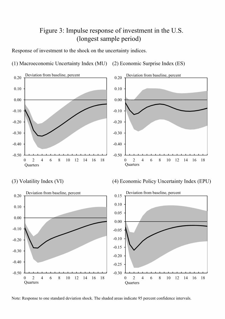
Figure 3: Impulse response of investment in the U.S. (longest sample period)

Response of investment to the shock on the uncertainty indices.

(1) Macroeconomic Uncertainty Index (MU) (2) Economic Surprise Index (ES)

(3) Volatility Index (VI) (4) Economic Policy Uncertainty Index (EPU)

Note: Response to one standard deviation shock. The shaded areas indicate 95 percent confidence intervals.

-0.50

-0.40

-0.30

-0.20

-0.10

0.00

0.10

0.20

0 2 4 6 8 10 12 14 16 18Quarters

Deviation from baseline, percent

-0.50

-0.40

-0.30

-0.20

-0.10

0.00

0.10

0.20

0 2 4 6 8 10 12 14 16 18


Quarters

-0.50

-0.40

-0.30

-0.20

-0.10

0.00

0.10

0.20

0 2 4 6 8 10 12 14 16 18


Quarters

-0.30

-0.25

-0.20

-0.15

-0.10

-0.05

0.00

0.05

0.10

0.15

0 2 4 6 8 10 12 14 16 18


Quarters

Figure 4: Impulse response of durable consumption in the U.S. (longest sample period)

Response of durable consumption to the shock on the uncertainty indices.




-0.30

-0.25

-0.20

-0.15

-0.10

-0.05

0.00

0.05

0.10

0.15

0.20

0 2 4 6 8 10 12 14 16 18


Quarters

-0.30

-0.20

-0.10

0.00

0.10

0.20

0.30

0 2 4 6 8 10 12 14 16 18


Quarters

-0.20

-0.15

-0.10

-0.05

0.00

0.05

0.10

0.15

0.20

0 2 4 6 8 10 12 14 16 18


Quarters

-0.15

-0.10

-0.05

0.00

0.05

0.10

0.15

0.20

0 2 4 6 8 10 12 14 16 18


Quarters

Figure 5: Impulse response of banks’ lending attitude in the U.S. (longest sample period)

Response of banks’ lending attitude to the shock on the uncertainty indices.



Note 1. Response to one standard deviation shock. The shaded areas indicate 95 percent confidence intervals. 2. The sign of the indicators for banks’ lending attitude is inverted.

-8.0

-6.0

-4.0

-2.0

0.0

2.0

4.0

6.0

0 2 4 6 8 10 12 14 16 18

DI, percent points

Tightened

Eased

Quarters

-6.0

-4.0

-2.0

0.0

2.0

4.0

6.0

8.0

0 2 4 6 8 10 12 14 16 18

DI, percent points

Tightened

Eased

Quarters

-6.0

-5.0

-4.0

-3.0

-2.0

-1.0

0.0

1.0

2.0

3.0

4.0

0 2 4 6 8 10 12 14 16 18

DI, percent points

Tightened

Eased

Quarters

-6.0

-5.0

-4.0

-3.0

-2.0

-1.0

0.0

1.0

2.0

3.0

4.0

0 2 4 6 8 10 12 14 16 18

DI, percent points

Tightened

Eased

Quarters

Figure 6: Impulse response of investment in Japan (longest sample period)





-0.20

-0.15

-0.10

-0.05

0.00

0.05

0.10

0 2 4 6 8 10 12 14 16 18


Quarters

-0.20

-0.15

-0.10

-0.05

0.00

0.05

0.10

0.15

0.20

0 2 4 6 8 10 12 14 16 18


Quarters

-0.20

-0.15

-0.10

-0.05

0.00

0.05

0.10

0.15

0.20

0 2 4 6 8 10 12 14 16 18


Quarters

-0.25

-0.20

-0.15

-0.10

-0.05

0.00

0.05

0.10

0 2 4 6 8 10 12 14 16 18


Quarters

Figure 7: Impulse responses of durable consumption in Japan (longest sample period)





-0.30

-0.20

-0.10

0.00

0.10

0.20

0.30

0 2 4 6 8 10 12 14 16 18


Quarters

-0.30

-0.20

-0.10

0.00

0.10

0.20

0.30

0 2 4 6 8 10 12 14 16 18


Quarters

-0.25

-0.20

-0.15

-0.10

-0.05

0.00

0.05

0.10

0.15

0 2 4 6 8 10 12 14 16 18


Quarters

-0.20

-0.10

0.00

0.10

0.20

0.30

0.40

0 2 4 6 8 10 12 14 16 18


Quarters

Figure 8: Impulse response of banks’ lending attitude in Japan (longest sample period)





-3.0

-2.0

-1.0

0.0

1.0

2.0

3.0

0 2 4 6 8 10 12 14 16 18

DI, percent points

Quarters

-3.0

-2.0

-1.0

0.0

1.0

2.0

3.0

0 2 4 6 8 10 12 14 16 18

DI, percent points

Quarters

-3.0

-2.0

-1.0

0.0

1.0

2.0

3.0

0 2 4 6 8 10 12 14 16 18

DI, percent points

Quarters

-5.0

-4.0

-3.0

-2.0

-1.0

0.0

1.0

2.0

3.0

0 2 4 6 8 10 12 14 16 18

DI, percent points

Quarters

Appendix Figure 1: Dataset for the Macroeconomic Uncertainty Index in Japan (67 series)

Note 1: The series are seasonally adjusted. 2: d = yt - yt-1, dlog = ln(yt) - ln(yt-1).

Group Name Unit

IIP :Production (Total) dlog

IIP :Production (Capital goods excluding Transport equipment) dlog

IIP :Production (Durable consumer goods) dlog

IIP :Production (Non-durable consumer goods) dlog

IIP :Production (Intermediate goods) dlog

IIP :Shipments (Total) dlog

IIP :Shipments (Capital goods excluding Transport equipment) dlog

IIP :Shipments (Durable consumer goods) dlog

IIP :Shipments (Non-durable consumer goods) dlog

IIP :Shipments (Intermediate goods) dlog

IIP :Inventory (Total) dlog

IIP :Inventory (Capital goods excluding Transport equipment) dlog

IIP :Inventory (Durable consumer goods) dlog

IIP :Inventory (Non-durable consumer goods) dlog

IIP :Inventory (Intermediate goods) dlog

Indices of Tertiary Industry Activity dlog

The number of effective job seekers dlog

The number of new job applications dlog

The number of effective job openings dlog

The number of new job openings dlog

Total cash earnings (Establishment with 30 or more employees) dlog

Total hours worked (Establishment with 30 or more employees) dlog

The number of new hires (Establishment with 30 or more employees) dlog

The number of total separations (Establishment with 30 or more employees) dlog

The number of employment dlog

The number of unemployment dlog

Value of exports dlog

Value of imports dlog

Value of exports to China dlog

Value of exports to the U.S. dlog

Export of Quantum Index dlog

Import of Quantum Index dlog

Real Exports dlog

Real Imports dlog

Production(16)

LaborMarket

(10)

Export andImport

(8)

Group Name Unit

Retail sales dlog

Sales of electronics and appliances retail stores dlog

New car registration dlog

Sales of department stores and supermarkets dlog

Sales of department stores dlog

Household spending index dlog

Construction starts (Private sector, non-residential,floor space)

dlog

Construction starts (Private sector, non-residential,estimated cost of construction)

dlog

New housing starts (Total) dlog

New housing starts (Owened) dlog

New housing starts (Rented) dlog

New housing starts (Built for sale) dlog

CPI (All items) dlog

CPI (All items, less fresh food) dlog

CPI (All items, less fresh food and energy) dlog

CPI (All items, less food and energy) dlog

Corporate Goods Price Index dlog

Nikkei Commodity Index (42 items) dlog

Nikkei Commodity Index (Textile) dlog

Nikkei Commodity Index (Steel products) dlog

Nikkei Commodity Index (Non-ferrous) dlog

Nikkei Commodity Index (Lumber) dlog

Nikkei Commodity Index (Chemical) dlog

Nikkei Commodity Index (Oil) dlog

Nikkei Commodity Index (Paper) dlog

Nikkei Commodity Index (Food) dlog

Nikkei Commodity Index (Other items) dlog

10-Year Government Bond Yields d

Call rate d

TOPIX dlog

Nominal effective exchange rate dlog

Exchange rate (USD/JPY) dlog

Money supply (M2) dlog

FinancialMarket

(6)

Consumption(6)

Investmentand

Housing(6)

Prices(15)

Appendix Figure 2: Impulse response of investment in the U.S. (from 2003/Q4)





-0.40

-0.30

-0.20

-0.10

0.00

0.10

0.20

0 2 4 6 8 10 12 14 16 18


Quarters

-0.50

-0.40

-0.30

-0.20

-0.10

0.00

0.10

0.20

0 2 4 6 8 10 12 14 16 18


Quarters

-0.50

-0.40

-0.30

-0.20

-0.10

0.00

0.10

0.20

0.30

0 2 4 6 8 10 12 14 16 18


Quarters

-0.30

-0.25

-0.20

-0.15

-0.10

-0.05

0.00

0.05

0.10

0.15

0.20

0 2 4 6 8 10 12 14 16 18


Quarters

Appendix Figure 3: Impulse response of durable consumption in the U.S. (from 2003/Q4)





-0.30

-0.25

-0.20

-0.15

-0.10

-0.05

0.00

0.05

0.10

0.15

0.20

0 2 4 6 8 10 12 14 16 18


Quarters

-0.30

-0.20

-0.10

0.00

0.10

0.20

0.30

0 2 4 6 8 10 12 14 16 18


Quarters

-0.20

-0.15

-0.10

-0.05

0.00

0.05

0.10

0.15

0 2 4 6 8 10 12 14 16 18


Quarters

-0.20

-0.15

-0.10

-0.05

0.00

0.05

0.10

0.15

0 2 4 6 8 10 12 14 16 18


Quarters

Appendix Figure 4: Impulse response of banks’ lending attitude in the U.S. (from 2003/Q4)




Note 1. Response to one standard deviation shock. The shaded areas indicate 95 percent confidence intervals. 2. The sign of the indicators for banks’ lending attitude is inverted.

-8.0

-6.0

-4.0

-2.0

0.0

2.0

4.0

6.0

0 2 4 6 8 10 12 14 16 18

DI, percent points

Tightened

Eased

Quarters

-6.0

-4.0

-2.0

0.0

2.0

4.0

6.0

8.0

0 2 4 6 8 10 12 14 16 18

Tightened

Eased

DI, percent points

Quarters

-5.0

-4.0

-3.0

-2.0

-1.0

0.0

1.0

2.0

3.0

4.0

5.0

0 2 4 6 8 10 12 14 16 18

Tightened

Eased

DI, percent points

Quarters

-6.0

-4.0

-2.0

0.0

2.0

4.0

6.0

0 2 4 6 8 10 12 14 16 18

Tightened

Eased

DI, percent points

Quarters

Appendix Figure 5: Impulse response of investment in Japan (from 2003/Q4)





-0.20

-0.15

-0.10

-0.05

0.00

0.05

0.10

0.15

0 2 4 6 8 10 12 14 16 18


Quarters

-0.20

-0.15

-0.10

-0.05

0.00

0.05

0.10

0.15

0.20

0 2 4 6 8 10 12 14 16 18


Quarters

-0.20

-0.15

-0.10

-0.05

0.00

0.05

0.10

0.15

0.20

0 2 4 6 8 10 12 14 16 18


Quarters

-0.15

-0.10

-0.05

0.00

0.05

0.10

0 2 4 6 8 10 12 14 16 18


Quarters

Appendix Figure 6: Impulse response of durable consumption in Japan (from 2003/Q4)





-0.30

-0.25

-0.20

-0.15

-0.10

-0.05

0.00

0.05

0.10

0.15

0 2 4 6 8 10 12 14 16 18


Quarters

-0.30

-0.20

-0.10

0.00

0.10

0.20

0.30

0 2 4 6 8 10 12 14 16 18


Quarters

-0.30

-0.25

-0.20

-0.15

-0.10

-0.05

0.00

0.05

0.10

0.15

0.20

0 2 4 6 8 10 12 14 16 18


Quarters

-0.25

-0.20

-0.15

-0.10

-0.05

0.00

0.05

0.10

0.15

0.20

0 2 4 6 8 10 12 14 16 18


Quarters

Appendix Figure 7: Impulse response of banks’ lending attitude in Japan (from 2003/Q4)





-3.0

-2.0

-1.0

0.0

1.0

2.0

3.0

0 2 4 6 8 10 12 14 16 18

DI, percent points

Quarters

-3.0

-2.0

-1.0

0.0

1.0

2.0

3.0

0 2 4 6 8 10 12 14 16 18

DI, percent points

Quarters

-3.0

-2.0

-1.0

0.0

1.0

2.0

3.0

0 2 4 6 8 10 12 14 16 18

DI, percent points

Quarters

-2.0

-1.5

-1.0

-0.5

0.0

0.5

1.0

1.5

2.0

2.5

3.0

0 2 4 6 8 10 12 14 16 18

DI, percent points

Quarters

(1) The EPU by country

(2) Subseries of the EPU in the U.S.

(3) Subseries of the EPU in Japan

Note 1: The global index is the weighted average of the EPU for 21 countries based on the PPP weights.

2: The indices are standardized. The dates of the latest figures are August 2020.

Appendix Figure 8: The EPUs

-2-10123456789

90 92 94 96 98 00 02 04 06 08 10 12 14 16 18 20

Global

United States

Japan

China

CY

-2-10123456789

90 92 94 96 98 00 02 04 06 08 10 12 14 16 18 20

Total

Monetary policy

Fiscal policy

Trade policy

CY

-2

-1

0

1

2

3

4

5

90 92 94 96 98 00 02 04 06 08 10 12 14 16 18 20

Total

Monetary policy

Fiscal policy

Trade policy

CY

Appendix Figure 9: EPUs and macroeconomic variables (i): VAR analysis (longest sample period)

(1) The U.S.

(2) Japan

Note 1: Global EPU is the weighted average of the EPU for 21 countries with PPP weights. 2: (+) and (−) indicate the positive and negative responses to the shock on the corresponding EPUs respectively. 3: ***, ** and * indicate statistically significant at 1, 5, and 10 percent significant levels, respectively.

percent

4 quartersahead

8 quartersahead

4 quartersahead

8 quartersahead

4 quartersahead

8 quartersahead

(－)*** 4 4 (－) 0 2 (－)*** 9 9

(－)*** 12 15 (－) 1 5 (－)*** 11 8

(－)*** 0 0 (+) 4 7 (－)*** 1 1

(－)*** 15 24 (－) 2 4 (－)*** 35 33

Fiscal policy (－)*** 11 20 (－) 2 5 (－)*** 33 33

Monetary policy (－)*** 4 8 (－) 2 2 (－)*** 15 15

Trade policy (－)*** 1 1 (－) 4 3 (+)*** 0 1


Impulseresponse

VarianceDecomposition Impulse

response


response

VarianceDecomposition

Global EPU

EPU for the U.S

EPU for China

EPU for Japan

percent

4 quartersahead

8 quartersahead

4 quartersahead

8 quartersahead

4 quartersahead

8 quartersahead

(－)*** 3 2 (－)*** 2 1 (－)*** 7 10

(－)*** 12 7 (－)*** 5 2 (－)*** 8 9

Fiscal policy (－)*** 8 5 (－)*** 4 3 (－)*** 2 4

Monetary policy (－)*** 6 3 (－)*** 10 5 (－)*** 11 10

Trade policy (+)*** 3 1 (－)*** 1 0 (+)*** 4 5

Banks’ lending attitude

Impulseresponse


response


response


Global EPU

EPU for the U.S

Investment Durable consumption

Appendix Figure 10: EPUs and macroeconomic variables (ii): VAR analysis (from 2003/Q4)

(1) The U.S.

(2) Japan

Note 1: Global EPU is the weighted average of the EPU for 21 countries with PPP weights. 2: (+) and (−) indicate the positive and negative responses to the shock on the corresponding EPUs respectively. 3: ***, ** and * indicate statistically significant at 1, 5, and 10 percent significant levels, respectively.

percent

4 quartersahead

8 quartersahead

4 quartersahead

8 quartersahead

4 quartersahead

8 quartersahead

(－)* 0 0 (－) 1 3 (－)*** 16 11

(－)* 5 4 (－) 5 7 (－)*** 26 13

(－)* 1 1 (－) 1 2 (－)*** 12 16

(－)* 7 6 (－) 2 6 (－)*** 8 4

Fiscal policy (－)* 8 10 (－) 2 9 (－)*** 10 6

Monetary policy (+)* 3 5 (－) 2 2 (－)*** 0 0

Trade policy (+)* 2 2 (－) 3 2 (－)*** 4 6


Impulseresponse


response


response


Global EPU

EPU for the U.S

EPU for China

EPU for Japan

percent

4 quartersahead

8 quartersahead

4 quartersahead

8 quartersahead

4 quartersahead

8 quartersahead

(－) 1 1 (－)** 0 0 (－)** 2 3

(－) 3 2 (－)** 1 1 (－)** 2 3

Fiscal policy (－) 0 1 (－)** 3 2 (+)** 8 8

Monetary policy (－) 3 3 (－)** 3 6 (－)** 9 8

Trade policy (－) 2 2 (－)** 0 0 (+)** 17 23

Banks’ lending attitude

Impulseresponse


response


response


Global EPU

EPU for the U.S

Investment Durable consumption

(1) Investment

(2) Durable consumption

Note 1: Global EPU is the weighted average of the EPU for 21 countries with PPP weights. 2: (+) and (−) indicate the positive and negative response to the shock on the uncertainty indices respectively. 3: ***, ** and * indicate statistically significant at 1, 5, and 10 percent significant levels, respectively.

Appendix Figure 11: The Uncertainty indices and macroeconomic variables (i): VAR analysis (longest sample period)

percent

4 quartersahead

8 quartersahead

4 quartersahead

8 quartersahead

4 quartersahead

8 quartersahead

4 quartersahead

8 quartersahead

MU (－)** 9 9 (－)*** 21 18 (－) * 2 3 (－)*** 37 32

ES (－)** 6 5 (－)*** 9 8 (－)* 9 12 (－)*** 4 5

VI (－)** 11 9 (－)*** 12 12 (－)* 1 1 (－)*** 5 10

EPU (－)** 2 4 (－)*** 1 5 (－)* 0 0 (－)*** 3 3

Global EPU (－)** 0 2 (－)*** 1 1 (－)* 5 6 (+)*** 4 6

Household spending (Durableconsumption)

Consumption Activity Index(Durable goods)

Electronic and appliance retailstores’ sales

New car registration

Impulseresponse

VarianceDecompositionImpulse

response


response


response


percent

4 quartersahead

8 quartersahead

4 quartersahead

8 quartersahead

4 quartersahead

8 quartersahead

4 quartersahead

8 quartersahead

4 quartersahead

8 quartersahead

4 quartersahead

8 quartersahead

MU (－)*** 17 13 (－)*** 19 18 (－)** 10 9 (－)*** 16 13 (－)** 4 7 (－)*** 19 16

ES (－)*** 2 1 (－)*** 1 1 (－)** 1 1 (－)*** 1 1 (－)** 9 8 (－)*** 3 1

VI (－)*** 24 17 (－)*** 51 35 (－)** 5 12 (－)*** 29 22 (－)** 4 4 (－)*** 7 4

EPU (－)*** 15 24 (－)*** 20 28 (－)** 4 11 (－)*** 9 9 (－)** 4 6 (－)*** 20 31

Global EPU (－)*** 4 4 (－)*** 7 7 (－)** 1 7 (－)*** 4 3 (－)** 1 1 (－)*** 4 5

Firms’ investment in FinancialStatements Statistics of

Corporations (All industries)

Impulseresponse


response


response


response


response

Construction starts (Privatesector, non-residential, the

estimate cost of construction)Variance

Decomposition Impulseresponse


Investment Supply of the capital goodsValue of construction put inplace (Private sector, non-

residential)Machinery orders

(1) Investment

(2) Durable consumption

Note 1: Global EPU is the weighted average of the EPU for 21 countries with PPP weights. 2: (+) and (−) indicate the positive and negative response to the shock on the uncertainty indices respectively. 3: ***, ** and * indicate statistically significant at 1, 5, and 10 percent significant levels, respectively.

Appendix Figure 12: The uncertainty indices and macroeconomic variables (ii): VAR analysis (from 2003/Q4)

percent

4 quartersahead

8 quartersahead

4 quartersahead

8 quartersahead

4 quartersahead

8 quartersahead

4 quartersahead

8 quartersahead

MU (－)** 10 8 (－)*** 21 18 (－)* 4 4 (－)*** 37 32

ES (－)** 6 5 (－)*** 9 8 (－)* 9 12 (－)*** 4 5

VI (－)** 12 10 (－)*** 12 12 (－)* 0 0 (－)*** 5 9

EPU (－)** 2 6 (－)*** 1 5 (－)* 5 5 (－)*** 6 6

Global EPU (－)** 1 3 (－)*** 0 1 (－)* 1 1 (+)*** 8 8

Household spending (Durableconsumption)

Consumption Activity Index(Durable goods)

Electronic and appliance retailstores’ sales

New car registration

Impulseresponse

VarianceDecompositionImpulse

response


response


response


percent

4 quartersahead

8 quartersahead

4 quartersahead

8 quartersahead

4 quartersahead

8 quartersahead

4 quartersahead

8 quartersahead

4 quartersahead

8 quartersahead

4 quartersahead

8 quartersahead

MU (－)*** 24 16 (－)*** 26 19 (－)*** 6 6 (－)*** 16 13 (－)** 12 14 (－)*** 16 12

ES (－)*** 2 1 (－)*** 1 1 (－)*** 1 1 (－)*** 1 1 (－)** 9 8 (－)*** 4 2

VI (－)*** 23 16 (－)*** 53 39 (－)*** 7 14 (－)*** 29 22 (－)** 4 4 (－)*** 7 4

EPU (－)*** 7 6 (－)*** 9 7 (－)*** 1 9 (－)*** 9 9 (－)** 2 3 (－)*** 2 5

Global EPU (－)*** 0 0 (－)*** 2 1 (－)*** 3 3 (－)*** 4 3 (－)** 1 1 (－)*** 7 4

Firms’ investment in FinancialStatements Statistics of

Corporations (All industries)

Impulseresponse


response


response


response


response

Construction starts (Privatesector, non-residential, the

estimate cost of construction)Variance

Decomposition Impulseresponse


Investment Supply of the capital goodsValue of construction put inplace (Private sector, non-

residential)Machinery orders

characteristics of uncertainty indices in the macroeconomy

Documents