characterization and erosion modeling of a nozzle-based

Characterization and Erosion Modeling ofa Nozzle-Based Inflow-Control Device

Jogvan J. Olsen and Casper S. Hemmingsen, Technical University of Denmark; Line Bergmann, Welltec;Kenny K. Nielsen and Stefan L. Glimberg, Lloyd’s Register Consulting—Energy; and

Jens H. Walther, Technical University of Denmark

Summary

In the petroleum industry, water-and-gas breakthrough in hydro-carbon reservoirs is a common issue that eventually leads touneconomic production. To extend the economic production life-time, inflow-control devices (ICDs) are designed to delay thewater-and-gas breakthrough. Because the lifetime of a hydrocar-bon reservoir commonly exceeds 20 years and it is a harsh envi-ronment, the reliability of the ICDs is vital.

With computational fluid dynamics (CFD), an inclined nozzle-based ICD is characterized in terms of the Reynolds number, dis-charge coefficient, and geometric variations. The analysis showsthat especially the nozzle edges affect the ICD flow characteris-tics. To apply the results, an equation for the discharge coefficientis proposed.

The Lagrangian particle approach is used to further investigatethe ICD. This allows for erosion modeling by injecting sand par-ticles into the system. By altering the geometry and modeling sev-eral scenarios while analyzing the erosion in the nozzles and atthe nozzle edges, an optimized design for incompressible media isfound. With a filleted design and an erosion-resistant material, themean erosion rate in the nozzles may be reduced by a factor ofmore than 2,500.

Introduction

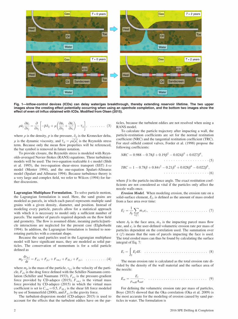
It is common to use long horizontal wells to increase reservoircontact and hydrocarbon recovery (Lien et al. 1991). Because hor-izontal wells typically have a higher production at the heel than atthe toe of the well as a result of uneven formation damage and thepressure difference in the long pipe, premature water or gas break-through is a common issue (Birchenko et al. 2010; Feng et al.2012). Eventually, because of the difference in density and viscos-ity of oil, water, and gas, cresting occurs, severely decreasinghydrocarbon production (Joshi 1991). Placing ICDs along thecompletion introduces a passively controlled pressure drop, andcan result in a more uniform influx along the completion. Thiscan significantly delay the cresting, and gives a potential for ahigher reservoir recovery. Fig. 1 illustrates how ICDs can extendreservoir lifetime compared with openhole completions.

Because a hydrocarbon reservoir is typically in production for5 to> 20 years (Garcia et al. 2009), the longtime reliability of thecompletion is important. Most ICDs have to be set to introducethe correct pressure drop before entering the well. Therefore, it isimportant that they can maintain their planned characteristics,because repairing or interchanging components in a well is oftennot a viable option. In particular, erosion and plugging can lead tothe deviation of the planned inflow profile (Visosky et al. 2007;Garcia et al. 2009). Because nozzle-based ICDs are prone to ero-sion (Zeng et al. 2013), their performance has to be known for alarge range of scenarios to ensure that the planned inflow charac-teristics will be maintained throughout the entire reservoir life-time. The current research on erosion of ICDs is outlined by Greciet al. (2014). They found five examples of experimental researchin which three experiments showed less than 6% change in pres-

sure drop, and two experiments showed no change. No previousresearch was found that showed erosion in ICDs analyzed by useof numerically simulated particles.

To prevent erosion from occurring in the ICDs, large particlesare filtered upstream from the flow with sand screens. Wheninvestigating erosion, the primary erosion factors are particle size,particle concentration, particle shape, particle velocity, angle ofimpact, and wall material (Coronado et al. 2009; Oka et al. 2009).For the present case, sand-particle sizes 100 to 1000 mm in diame-ter are investigated. The larger particles can penetrate the sandscreen initially, whereas only the smaller particles will passthrough after a natural sandpack has built up on the sand screen(Feng et al. 2012). In addition, Zamberi et al. (2014) show thatsand-screen erosion can occur, allowing the large sand particlesto pass through.

The nozzle-based ICDs have been deployed in wells since2015, for operators in West Africa and operators in the MiddleEast. The applications have been different: Some were installed touse the ICDs in the application as gas lift valve and some in theapplication as zonal-production valve. Since the end of 2016,more than 35 ICDs have been installed and used in wells, andmore than 250 valves have been ordered. The objective of this pa-per is to use numerical methods to characterize and investigateerosion for a nozzle-based ICD with varying geometry. The pur-pose is to optimize the ICD in terms of erosion to improve long-time performance and to present the results with simple equationsready to implement in reservoir simulators.

CFD Formulation

With CFD, the ICD can be analyzed for a range of scenarios byspatially discretizing the domain and solving the fundamentalfluid-dynamics equations. This allows for numerically analyzingthe ICD in terms of flow characteristics and erosion rates.

Fundamental Equations for Incompressible Flow. The govern-ing equations for solving the flow are the Navier-Stokes and conti-nuity equations. Because the maximum simulated pressuredifference will be Dp ¼ 20 bar, gas release and viscosity changesare assumed negligible. In addition, with data from Lien et al.(1991), the change in density is only 1.7 kg/m3 (0.2%) at Dp ¼ 20bar, meaning the oil can be assumed incompressible. To savecomputational time, the steady-state solution can be found. Thegoverning equations are modeled by splitting the velocity ui into amean (ui) and a fluctuating component (u0i),

ui ¼ ui þ u0i; ð1Þ

here written in Einstein notation.The mean continuity equation for an incompressible fluid is

@uj

@xj¼ 0; ð2Þ

where uj is the velocity vector and xj denotes the spatialcoordinate.

The incompressible time-averaged Navier-Stokes equation(White 2006) for solving the fluid momentum is

. . . . . . . . . . . . . . . . . . . . . . . . . . . . . .

. . . . . . . . . . . . . . . . . . . . . . . . . . . . . . . . .

Copyright VC 2017 Society of Petroleum Engineers

Original SPE manuscript received for review 7 February 2016. Revised manuscript receivedfor review 11 February 2017. Paper (SPE 186090) peer approved 16 February 2017.

DC186090 DOI: 10.2118/186090-PA Date: 8-May-17 Stage: Page: 1 Total Pages: 10

ID: jaganm Time: 16:39 I Path: S:/DC##/Vol00000/170014/Comp/APPFile/SA-DC##170014

2016 SPE Drilling & Completion 1

quj@ui

@xj¼ @

@xj�pdij þ l

@ui

@xjþ @uj

@xi

� �� sij

� �; ð3Þ

where q is the density, p is the pressure, dij is the Kronecker delta,

l is the dynamic viscosity, and sij ¼ qu0iu0j is the Reynolds stress

term. Because only the mean flow properties will be referenced,the bar symbol is removed in future notation.

To provide closure, the Reynolds stress is modeled with Reyn-olds-averaged Navier-Stokes (RANS) equations. Three turbulencemodels will be used: The two-equation realizable k-e model (Shihet al. 1995), the two-equation shear-stress transport (SST) k-xmodel (Menter 1994), and the one-equation Spalart-Allmarasmodel (Spalart and Allmaras 1994). Because turbulence theory isa very large and complex field, we refer to Wilcox (1994) for fur-ther discussions.

Lagrangian Multiphase Formulation. To solve particle motion,the Lagrangian formulation is used. Here, the sand grains aremodeled as parcels, in which each parcel represents multiple sandgrains with a given density, diameter, and position. Instead ofmodeling every particle, parcels allow for a statistical approachwith which it is necessary to model only a sufficient number ofparcels. The number of parcels required depends on the flow fieldand geometry. The flow is assumed dilute, meaning particle/parti-cle interactions are neglected for the present case (Elghobashi1994). In addition, the Lagrangian formulation is limited to non-rotating particles with a constant shape.

Because the sand particles used in the Lagrangian multiphasemodel will have significant mass, they are modeled as solid par-ticles. The conservation of momentum is for a solid particledefined as

mpdvp;i

dt¼ Fd;i þ Fp;i þ Fvm;i þ FSL;i þ Fg;i; ð4Þ

where mp is the mass of the particle, vp,i is the velocity of the parti-cle, Fd,i is the drag force defined with the Schiller-Naumann corre-lation (Schiller and Naumann 1933), Fp,i is the pressure-gradientforce provided by CD-adapco (2015), Fvm,i is the virtual massforce provided by CD-adapco (2015) in which the virtual masscoefficient is set to Cvm¼ 0.5, FSL,i is the shear lift force modeledby use of Sommerfeld (2000), and Fg,i is the gravity force.

The turbulent-dispersion model (CD-adapco 2015) is used toaccount for the effects that the turbulent eddies have on the par-

ticles, because the turbulent eddies are not resolved when using aRANS model.

To calculate the particle trajectory after impacting a wall, theparticle-restitution coefficients are set for the normal restitutioncoefficient (NRC) and the tangential restitution coefficient (TRC).For steel oilfield control valves, Forder et al. (1998) propose thefollowing coefficients:

NRC ¼ 0:988� 0:78bþ 0:19b2 � 0:024b3 þ 0:027b4;

� � � � � � � � � � � � � � � � � � � ð5Þ

TRC ¼ 1� 0:78bþ 0:84s2 � 0:21b3 þ 0:028b4 � 0:022b5;

� � � � � � � � � � � � � � � � � � � ð6Þ

where b is the particle-incidence angle. The exact restitution coef-ficients are not considered as vital if the particles only affect thenozzle walls once.

Erosion Model. When modeling erosion, the erosion rate on asolid-surface element, Ef, is defined as the amount of mass erodedfrom a face area over time:

Ef ¼1

Af

Xpðf Þ

_mper; ð7Þ

where Af is the face area, _mp is the impacting parcel mass flowrate, and er is the user-defined volumetric erosion rate per mass ofparticles dependent on the correlation used. The summation overp ( f ) means that the sum of parcels impacting the face is used.The total eroded mass can thus be found by calculating the surfaceintegral of Eq. 7:

Et ¼ð

S

Ef dS: ð8Þ

The mean erosion rate is calculated as the total erosion rate di-vided by the density of the wall material and the surface area ofthe nozzle:

Em ¼Et

qwallAsurf

: ð9Þ

For defining the volumetric erosion rate per mass of particles,Boye (2015) showed that the Oka correlation (Oka et al. 2009) isthe most accurate for the modeling of erosion caused by sand par-ticles in water. The formulation is

. . . . . . .

. . . . . . . . . .

. . . . . . . . . . . . . . . . . . . . . . . . . .

. . . . . . . . . . . . . . . . . . . . . . . . . . . . .

. . . . . . . . . . . . . . . . . . . . . . . . . . .

Gas

ToeOil

ToeSandscreenOil

Heel

Heel

Water

Water

Gas

ICD

T = 0 years

T = 0 years

Gas

ToeOil

ToeSandscreenOil

Heel

Heel

Water

Water

Gas

ICD

T = 2 years

T = 2 years

Fig. 1—Inflow-control devices (ICDs) can delay water/gas breakthrough, thereby extending reservoir lifetime. The two upperimages show the cresting effect potentially occurring when using an openhole completion, and the bottom two images show theeffect of even oil influx obtained with ICDs. Modified from Olsen (2015).



2 2016 SPE Drilling & Completion

er ¼ e90gðbÞ jvpjvref

� �k1 dp

dref

� �k2

; ð10Þ

where g(b) is the impact-angle dependence:

gðbÞ ¼ ðsinbÞn1 ½1þ Hvð1� sinbÞ�n2 ð11Þ

Here, n1, n2, k1, and k2 are user-defined constants, and b is the par-ticle-impact angle on the surface. vref and dref are the specified ref-erence particle velocity and diameter on the basis of the chosenexperiment used for finding the appropriate coefficients. Here, theflat-plate experiment by Zhang et al. (2007) was used. e90 is thereference volumetric erosion rate per mass of particles at a 90

�

impact angle. Oka et al. (2009) show that the term ðsinbÞn1 in Eq.11 is associated with the brittle characteristics of the wall material,whereas the second term ½1þ Hvð1� sinbÞ�

n2is associated with

the cutting action. The cutting action is the most relevant whenworking with low impact angles. Plotting the g(b) term in Eq. 11for the two materials (Fig. 2) shows that the harder tungsten car-bide is only slightly more prone to erosion at low-impact anglescompared with steel. Fig. 2 also shows that, at high impact angles,the tungsten carbide performs significantly better than steel. Thefigure also shows that the erosion will rapidly decrease for higherimpact angles by use of tungsten carbide instead of steel.

Characterizing the ICD

Because the purpose of using ICDs is to control the reservoirinflux, the flow properties of the ICDs are of interest. By charac-terizing the ICD in terms of the discharge coefficient and Reyn-olds number, the relationship between the pressure difference and

flow rate is found for different scenarios. This gives the opportu-nity for quickly analyzing a reservoir on the basis of nodal-approach methods as described by Johansen and Khoriakov(2007) or by implementing the characteristics as sink terms in aCFD model. The nozzle Reynolds number is

Re ¼ qunl

l¼ unl

�; ð12Þ

where un is the mean nozzle flow velocity, l is the characteristiclength scale, and Re is Reynolds number. The characteristiclength scale for the ICD is the nozzle diameter, dn. The Reynoldsnumber allows for scaling the results on the basis of the four pa-rameters in Eq. 12.

The discharge coefficient is used to compare the actual com-puted flow rate with the theoretical Bernoulli flow rate,

Cd ¼_m

Affiffiffiffiffiffiffiffiffiffiffi2qDpp ; ð13Þ

where Dp is the pressure drop across the nozzle, A is the minimumnozzle flow area, and _m is the nozzle mass flow rate.

The present ICD is nozzle-based, with a binary shutdownmechanism [refer to Olsen (2015) for details] designed to closesections of the well in the event of premature breakthrough. Thenozzles are inclined at a 30� angle, and by default, four nozzlesare used, each with 6-mm diameter and equally spaced around thecircumference. Olsen (2015) showed that it is not required tomodel the reservoir when analyzing the ICD placed in a permea-ble reservoir, because the reservoir does not significantly alter theinflow-velocity profile. The simulated domain consists thereforeof the wellbore, ICD, and production well with the dimensionsand boundary conditions shown in Fig. 3.

Zeng et al. (2013) showed that the restrictive pressure-dropcharacteristics for a nozzle-based ICD are

Dpr / qu2n; ð14Þ

meaning that the pressure difference across the ICD is independ-ent of viscosity. This is because the friction losses are muchsmaller than the restrictive losses.

The oil properties are assumed as loil ¼ 15 cp and qoil ¼ 850kg/m3. To model a real oil well, it is assumed that the well pro-duction is _mprod ¼ 5 kg/s (equal to 508 m3/d), and the nozzle flowrate is governed by the well and wellbore-pressure difference. Forthe analysis, only the mass flow rate through the nozzles is used.For modeling turbulence, the realizable k-e model (Shih et al.1995) is used.

The ICD flow characteristics can be found by simulating overa range of pressure differences. Olsen (2015) shows that, particu-larly, the fillets have a large impact on the mass flow rate. There-fore, the range Dp ¼ 0:1–20 bar is simulated for varying filletradii. A mesh independence study was performed to ensure a

. . . . . . . . . . . . . . . .

. . . . . . . . . . . . .

. . . . . . . . . . . . . . . . . . . . . . . . . .

. . . . . . . . . . . . . . . . . . . . . . . . . . .

. . . . . . . . . . . . . . . . . . . . . . . . . . . . . .

00

0.2

0.4

0.6

0.8

1

20

Steel

Tungsten carbide

40 60

Imapact Angle, β (degrees)

Nor

mal

ized

g (β)

80

Fig. 2—Impact-angle dependence as a function of particle-impact angle with Eq. 11. Both graphs are normalized totheir respective maximum value, g(b)max,steel 5 1.35 andg(b)max,tungsten 5 6.72. Hv,steel 5 2.354 GPa, and Hv,tungsten 5 17.65GPa.

φ6-mm nozzle

Closing mechanismWell outletBC: Pressure outletValue: 0 bar

Well inletBC: Mass flow rate

Value: 5 kg/s

Left reservoir inletBC: Pressure inletValue: 10 bar

746.0

φ190

.5φ1

41.5

φ127

.0φ1

00.5

φ100

.5

φ120

.5

φ100

.5

Right reservoir inletBC: Pressure inlet

Value: 10 bar

Fig. 3—Fluid domain of the assumed scenario along with the boundary conditions (BCs). All surfaces with no specified BC aremodeled as walls with a no-slip condition. The green arrows show the reservoir flow, and the blue arrows show the production-well flow. All units are in millimeters. From Olsen (2015).




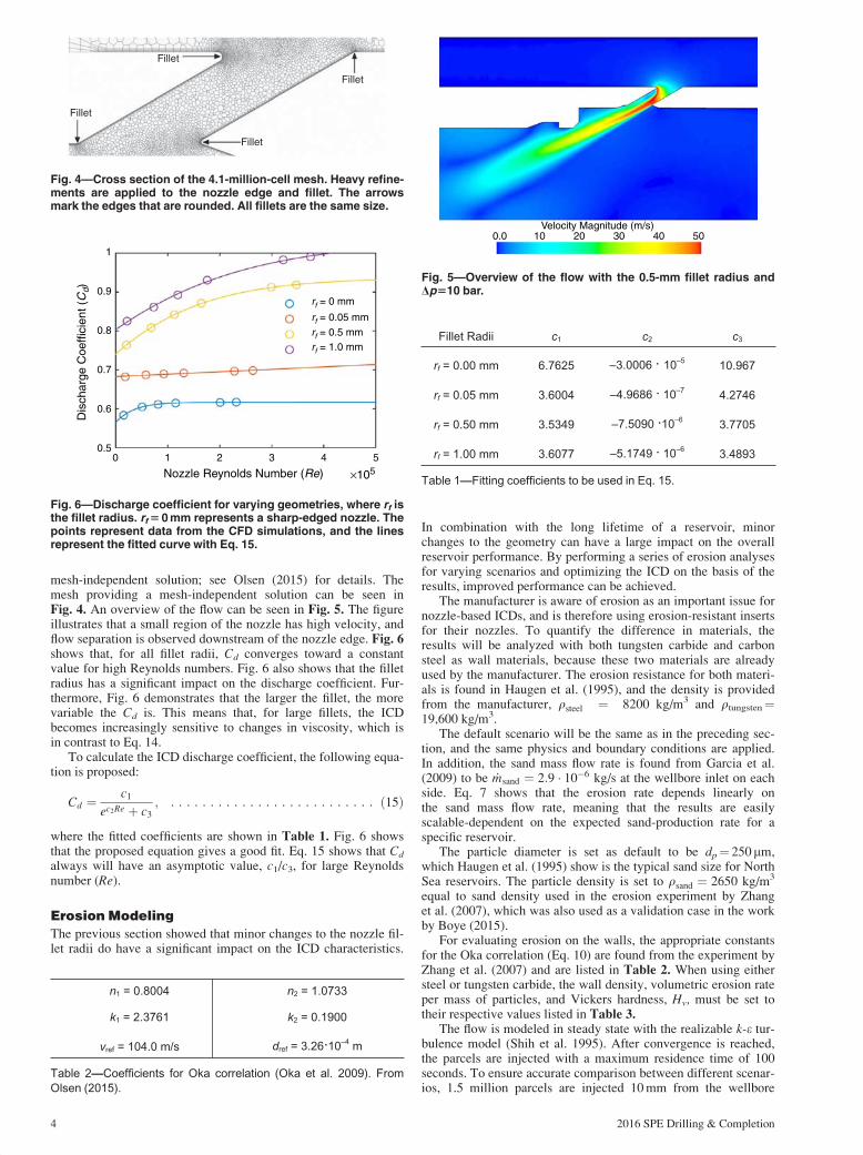
mesh-independent solution; see Olsen (2015) for details. Themesh providing a mesh-independent solution can be seen inFig. 4. An overview of the flow can be seen in Fig. 5. The figureillustrates that a small region of the nozzle has high velocity, andflow separation is observed downstream of the nozzle edge. Fig. 6shows that, for all fillet radii, Cd converges toward a constantvalue for high Reynolds numbers. Fig. 6 also shows that the filletradius has a significant impact on the discharge coefficient. Fur-thermore, Fig. 6 demonstrates that the larger the fillet, the morevariable the Cd is. This means that, for large fillets, the ICDbecomes increasingly sensitive to changes in viscosity, which isin contrast to Eq. 14.

To calculate the ICD discharge coefficient, the following equa-tion is proposed:

Cd ¼c1

ec2Re þ c3

; ð15Þ

where the fitted coefficients are shown in Table 1. Fig. 6 showsthat the proposed equation gives a good fit. Eq. 15 shows that Cd

always will have an asymptotic value, c1/c3, for large Reynoldsnumber (Re).

Erosion Modeling

The previous section showed that minor changes to the nozzle fil-let radii do have a significant impact on the ICD characteristics.

In combination with the long lifetime of a reservoir, minorchanges to the geometry can have a large impact on the overallreservoir performance. By performing a series of erosion analysesfor varying scenarios and optimizing the ICD on the basis of theresults, improved performance can be achieved.

The manufacturer is aware of erosion as an important issue fornozzle-based ICDs, and is therefore using erosion-resistant insertsfor their nozzles. To quantify the difference in materials, theresults will be analyzed with both tungsten carbide and carbonsteel as wall materials, because these two materials are alreadyused by the manufacturer. The erosion resistance for both materi-als is found in Haugen et al. (1995), and the density is providedfrom the manufacturer, qsteel ¼ 8200 kg/m3 and qtungsten¼19,600 kg/m3.

The default scenario will be the same as in the preceding sec-tion, and the same physics and boundary conditions are applied.In addition, the sand mass flow rate is found from Garcia et al.(2009) to be _msand ¼ 2:9 � 10�6 kg/s at the wellbore inlet on eachside. Eq. 7 shows that the erosion rate depends linearly onthe sand mass flow rate, meaning that the results are easilyscalable-dependent on the expected sand-production rate for aspecific reservoir.

The particle diameter is set as default to be dp¼ 250mm,which Haugen et al. (1995) show is the typical sand size for NorthSea reservoirs. The particle density is set to qsand ¼ 2650 kg/m3

equal to sand density used in the erosion experiment by Zhanget al. (2007), which was also used as a validation case in the workby Boye (2015).

For evaluating erosion on the walls, the appropriate constantsfor the Oka correlation (Eq. 10) are found from the experiment byZhang et al. (2007) and are listed in Table 2. When using eithersteel or tungsten carbide, the wall density, volumetric erosion rateper mass of particles, and Vickers hardness, Hv, must be set totheir respective values listed in Table 3.

The flow is modeled in steady state with the realizable k-e tur-bulence model (Shih et al. 1995). After convergence is reached,the parcels are injected with a maximum residence time of 100seconds. To ensure accurate comparison between different scenar-ios, 1.5 million parcels are injected 10 mm from the wellbore

. . . . . . . . . . . . . . . . . . . . . . . . . .

Fillet

Fillet

Fillet

Fillet

Fig. 4—Cross section of the 4.1-million-cell mesh. Heavy refine-ments are applied to the nozzle edge and fillet. The arrowsmark the edges that are rounded. All fillets are the same size.

0.0 10 20Velocity Magnitude (m/s)

30 40 50

Fig. 5—Overview of the flow with the 0.5-mm fillet radius andDp510 bar.

00.5

0.6

0.7

0.8

rf = 0 mm

rf = 0.05 mm

rf = 0.5 mmrf = 1.0 mm

0.9

1

1 2

Nozzle Reynolds Number (Re)

Dis

char

ge C

oeffi

cien

t (C

d)

3 4 5

×105

Fig. 6—Discharge coefficient for varying geometries, where rf isthe fillet radius. rf 5 0 mm represents a sharp-edged nozzle. Thepoints represent data from the CFD simulations, and the linesrepresent the fitted curve with Eq. 15.

Fillet Radii c1 c2 c3

rf = 0.00 mm 6.7625 –3.0006 · 10–5 10.967

rf = 0.05 mm 3.6004 –4.9686 · 10–7 4.2746

rf = 0.50 mm 3.5349 –7.5090 ·10–6 3.7705

rf = 1.00 mm 3.6077 –5.1749 · 10–6 3.4893

Table 1—Fitting coefficients to be used in Eq. 15.

n1 = 0.8004 n2 = 1.0733

k1 = 2.3761 k2 = 0.1900

vref = 104.0 m/s dref = 3.26·10–4 m

Table 2—Coefficients for Oka correlation (Oka et al. 2009). From

Olsen (2015).




inlets with an equidistant spacing between each parcel. Further-more, a new mesh-independence analysis is performed for theerosion analysis to ensure a mesh-independent solution, whichresulted in a mesh containing 16.0 million cells; see Olsen (2015)for details.

Erosion Results. The erosion aspects are analyzed by investigat-ing the erosion pattern and the mean erosion rate in the nozzles.To ensure an accurate mean, the results from all four nozzles areused when discussing the mean erosion rate.

Fig. 7a shows the initial results for the default scenario withsteel nozzles. The erosion results demonstrate that there is a local-ized erosion at the center of the nozzles. Fig. 8 shows the tangen-tial in-plane velocity contours and the location of the particleswith the sharp-edged nozzle; see Fig. 9 for reference coordinatesystem. The results show strong secondary flow structures in theentrance of the nozzle, contributing to the displacement of theparticles toward the wall. By minimizing the separation, thestrength of the secondary flow should decrease, lowering the ero-

sion rate. The figure also shows that the secondary flows are notsymmetric until after L/d¼ 2, meaning that the erosion is notentirely symmetrical. In addition, Fig. 8 shows that the particlesare densely packed when impacting the nozzle wall. This mightinterfere locally with the dilute assumption, and can be a sourceof inaccuracy leading to overestimated erosion rates becausesome particles do not collide with the wall but with each other,which is not modeled.

Because the predicted mean erosion rate is Em;steel ¼ 0:47 mm/a, optimizing the nozzles is important if the planned inflow char-acteristics should be maintained. With the assumption that thepressure drop should not change more than 5%, the simulatedICD lifetime will be less than 6 months.

Fig. 7b shows the erosion with tungsten carbide. Comparingthe mean erosion rate for the two materials gives a factor of 29 indifference, which equals a lifetime of 14 years. The figure showsa very similar erosion pattern for the two materials. Fig. 10 showsthe particle-impact angle. It is observed that 95% of the particleshave an impact angle less than 12.5�. The nearly identical erosionpattern is a result of the normalized g(b) shown in Fig. 2 beingnearly identical for the two materials at low angles. Furthermore,this shows that, if further erosion resistance should be achieved, amaterial resistant to the cutting action should be found.

Material e90 Hv ρwall

Steel 1.76 ·10–3 m3/kg 2.354 GPa 8200 kg/m3

Tungsten 2.40 · 10–5 m3/kg 17.65 GPa 19600 kg/m3

Table 3—Wall-material properties. From Olsen (2015).

0.0Erosion (mm/a)

0.8 1.6 3.2 4.0

(a)

0.0Erosion (mm/a)

0.025 0.050 0.075 0.10

(b)

Fig. 7—Close-up view of the nozzle erosion rate with steel (a)and tungsten carbide (b), respectively. Notice the change inscale. The mean erosions for the nozzles were Em,steel 50.47 mm/a and Em,tungsten 5 0.016 mm/a.

L/d = 0.50 L/d = 0.75

L/d = 1.00 L/d = 1.25

L/d = 1.50 L/d = 2.00

0 10 20 30

y1z1

40 50 60

Fig. 8—Tangential velocity contour (m/s) in the [x1, y1, z1] coor-dinate system for the sharp-edged nozzle. The white circlesrepresent the particle position. The high-velocity secondaryflows pull the particles toward the nozzle edge, causingerosion.

0.0 0.8Erosion (mm/a)

1.6 3.2 4.0

y1

z1x1

L /d = 2.00

L /d = 1.50L /d = 1.25

L /d = 1.00L /d = 0.75

L /d = 0.50

Fig. 9—Position of local coordinate system and velocity planes.The local coordinate-system origin is placed at the center ofthe nozzle inlet with x1 parallel to the nozzle. L is the positiondown the x1-axis, and d is the nozzle diameter. The black arrowrepresents the view direction used in Fig. 18.




The nozzle edge is also investigated. It shows that the erosionrates were exceeding 0.1 mm/a and 4.0 mm/a at several locationson the nozzle edge for tungsten carbide and steel, respectively.This means that, after only a short time, flow characteristics of thenozzles will change.

Because using tungsten-carbide nozzles gives a large improve-ment in comparison to steel nozzles, the remaining erosion simu-lations will be made with tungsten carbide as wall material.

Sensitivity to Turbulence Models. Because the behavior ofthe separation in the nozzle is highly influenced by the choice ofturbulence model, three standard turbulence models are comparedin terms of erosion rate. Fig. 11 shows the erosion prediction forthe realizable k-e model, the Spalart-Allmaras model, and the k-xSST model. The figure shows that the realizable k-e model has amuch sharper erosion pattern in comparison with the two otherturbulence models. It is noticed that the Spalart-Allmaras modeland the k-x SST model show similar erosion patterns. Because ofthe uncertainties associated with erosion modeling and the lack ofexperimental work for inclined nozzles, no conclusions can bemade on which model performs best. The two largest uncertain-ties come from imperfect solutions to the flow field, resulting inthe particle trajectory being incorrect and in the uncertainty of theerosion-model coefficients. In the validation case by Zhang et al.(2007), they found the deviation in erosion to be 0–25% withwater. Because the computational mesh is significantly finerfor the present case, the deviation can thus not be expected toexceed 25%.

To model the effect of turbulent fluctuation on the particle tra-jectory, the turbulent-dispersion model is used. Activating the tur-bulent-dispersion model results in the parcel trajectory becomingmore chaotic downstream of the nozzles. It is contrary that theparticle trajectory before entering the nozzles is very similar, indi-cating few flow fluctuations in the wellbore. The parcel trajectoryin the nozzles (Fig. 12) shows that the behavior is similar withand without turbulent dispersion. Because erosion is onlyexpected in the nozzle wall and nozzle edges, the turbulent-dis-persion model can therefore only be expected to have a minorimpact on the mean erosion rate.

Fig. 13 shows the erosion pattern with the turbulent-dispersionmodel. The erosion pattern becomes more diffused when turbu-lent dispersion is activated, but there is only a 2.5% difference inmean erosion rate. In terms of usability, it is more attractive torun the simulations without turbulent dispersion, because a clearerosion pattern is preferred for analysis. In addition, the turbulent-dispersion model increases the simulation time by more than afactor of 2. Therefore, the turbulent-dispersion model will not beused for the remaining simulations.

Parametric Analysis of Eroding Factors. The type of sandscreen used will vary depending on the specific reservoir becausethe sand-grain size is reservoir-dependent. Therefore, simulationsare performed with the particle-grain sizes of 100, 250, 500, and1000 mm in diameter. Fig. 14 demonstrates that the larger the par-ticles are, the higher up the nozzle the erosion starts. Furthermore,almost no erosion can be observed for very small particles. Noticethat the erosion rate does not necessarily increase with the parti-cle-grain size, but does instead have a maximum erosion ratewhen using 500-mm particles. This must be because of the largerparticles impacting the nozzles at either small angles or largeangles, resulting in lower erosion rates; see Fig. 2.

To investigate how the erosion will vary for differentflow velocities, the pressure difference across the nozzle is varied.Fig. 15 shows the erosion for Dp ¼ 5 bar, Dp ¼ 10 bar, and Dp ¼20 bar. Notice that the erosion pattern has a similar shape for thethree cases. The difference is that, for larger Dp, the erosion rateis higher and starts higher up the nozzle. This indicates that thesecondary flows behave identically for all three cases, with the

0 5 10

Impact Angle (deg)15 20

Fig. 10—Particle-impact angle in the nozzle. The mean particle-impact angle is 9.48. 95% of the particles have an impact angle<12.58. Zero impact angle represents regions where no particleimpacts are observed.

0.0Erosion (mm/a)

0.025 0.050 0.075 0.1

Fig. 11—Turbulence models used from left to right: the realiz-able k-e model, the Spalart-Allmaras model, and the k-x SSTmodel. The mean erosion is Em;k�e50:016 mm/a, Em,S-A 50.013 mm/a, and Em,k-x 5 0.012 mm/a. The material is tungstencarbide.

0.0 8.0 16Velocity Magnitude (m/s)

24 32 40

Fig. 12—Particle trajectory in the nozzle. The turbulent-disper-sion model is activated on the right image. The particle trajec-tory can be seen to be only slightly wider when the turbulentdispersion is activated. From Olsen (2015).

0.0Erosion (mm/a)

0.025 0.050 0.075 0.10

Fig. 13—Comparison of the erosion pattern without (left) andwith (right) turbulent dispersion. The patterns are very similarexcept that the turbulent-dispersion model results in a more-diffused erosion pattern. The mean erosion rates areEm,default 5 0.016 mm/a and Em,turbulent 5 0.016 mm/a. The maxi-mum erosion is lower with the turbulent-dispersion model,because fewer particles affect the exact same location on thewall. The material is tungsten carbide.

0.0Erosion (mm/a)

0.025 0.050 0.075 0.10

Fig. 14—Particle size used from left to right: 100, 250, 500, and1000 lm. The mean erosion rate is Em,100 lm 5 0.0016 mm/a,Em,250 lm 5 0.016 mm/a, Em,500 lm 5 0.031 mm/a, and Em,1000 lm 50.019 mm/a. The material is tungsten carbide without the turbu-lent-dispersion model.




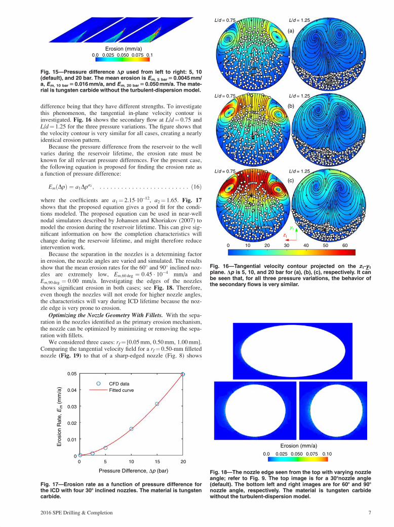
difference being that they have different strengths. To investigatethis phenomenon, the tangential in-plane velocity contour isinvestigated. Fig. 16 shows the secondary flow at L/d¼ 0.75 andL/d¼ 1.25 for the three pressure variations. The figure shows thatthe velocity contour is very similar for all cases, creating a nearlyidentical erosion pattern.

Because the pressure difference from the reservoir to the wellvaries during the reservoir lifetime, the erosion rate must beknown for all relevant pressure differences. For the present case,the following equation is proposed for finding the erosion rate asa function of pressure difference:

EmðDpÞ ¼ a1Dpa2 ; ð16Þ

where the coefficients are a1¼ 2.15�10–12, a2¼ 1.65. Fig. 17shows that the proposed equation gives a good fit for the condi-tions modeled. The proposed equation can be used in near-wellnodal simulators described by Johansen and Khoriakov (2007) tomodel the erosion during the reservoir lifetime. This can give sig-nificant information on how the completion characteristics willchange during the reservoir lifetime, and might therefore reduceintervention work.

Because the separation in the nozzles is a determining factorin erosion, the nozzle angles are varied and simulated. The resultsshow that the mean erosion rates for the 60� and 90� inclined noz-zles are extremely low, Em;60 deg ¼ 0:45 � 10�4 mm/a andEm;90 deg ¼ 0:00 mm/a. Investigating the edges of the nozzlesshows significant erosion in both cases; see Fig. 18. Therefore,even though the nozzles will not erode for higher nozzle angles,the characteristics will vary during ICD lifetime because the noz-zle edge is very prone to erosion.

Optimizing the Nozzle Geometry With Fillets. With the sepa-ration in the nozzles identified as the primary erosion mechanism,the nozzle can be optimized by minimizing or removing the sepa-ration with fillets.

We considered three cases: rf¼ [0.05 mm, 0.50 mm, 1.00 mm].Comparing the tangential velocity field for a rf¼ 0.50-mm filletednozzle (Fig. 19) to that of a sharp-edged nozzle (Fig. 8) shows

. . . . . . . . . . . . . . . . . . . . . . . . .

0.0Erosion (mm/a)

0.025 0.050 0.075 0.1

Fig. 15—Pressure difference Dp used from left to right: 5, 10(default), and 20 bar. The mean erosion is Em, 5 bar 5 0.0045 mm/a, Em, 10 bar 5 0.016 mm/a, and Em, 20 bar 5 0.050 mm/a. The mate-rial is tungsten carbide without the turbulent-dispersion model.

L/d = 0.75 L/d = 1.25

(a)

(b)

(c)

0 10 20 30

z1

y1

40 50 60

L/d = 0.75 L/d = 1.25

L/d = 0.75 L/d = 1.25

Fig. 16—Tangential velocity contour projected on the z1-y1

plane. Dp is 5, 10, and 20 bar for (a), (b), (c), respectively. It canbe seen that, for all three pressure variations, the behavior ofthe secondary flows is very similar.

00

0.01

0.02

0.03

0.04

0.05

CFD dataFitted curve

5 10

Pressure Difference, Δp (bar)

Ero

sion

Rat

e, E

m (

mm

/a)

15 20

Fig. 17—Erosion rate as a function of pressure difference forthe ICD with four 308 inclined nozzles. The material is tungstencarbide.

0.0

Erosion (mm/a)

0.025 0.050 0.075 0.10

Fig. 18—The nozzle edge seen from the top with varying nozzleangle; refer to Fig. 9. The top image is for a 308nozzle angle(default). The bottom left and right images are for 608 and 908nozzle angle, respectively. The material is tungsten carbidewithout the turbulent-dispersion model.




that the fillets greatly reduce the secondary flows, resulting in lessdisplacement of the particles toward the wall and, hence, less ero-sion. In addition, this implies that the erosion rate will decelerateover time for the sharp-edged nozzle.

The erosion pattern can be seen in Fig. 20. For the rf¼ 0.05-mmfillet, a minor improvement is seen because the mean erosion ratehas decreased from Em,sharp¼ 0.016 mm/a to Em,rf 005¼0.011 mm/a. Using fillets that are either rf¼ 0.50 mm or rf¼1.00 mm shows a major improvement with the mean erosion rate asEm,rf 050¼ 1.8�10–4 mm/a and Em,rf 100¼ 2.1�10–4 mm/a, respec-tively. This means that, according to the simulations, a reductionfactor of 89 in erosion rate can be achieved with 0.5-mm fillets.

By applying the erosion-resistant tungsten carbide and using a0.5-mm fillet on the nozzle edges, a reduction factor of 2,612in ero-sion rate is simulated in comparison to the standard sharp-edgedsteel nozzle. This may increase significantly the accuracy of theflow characteristics during the reservoir lifetime, because the mod-eled ICD lifetime is now 1,235 years at Dp ¼ 10 bar. With Eq. 16,this could be translated into 20 years, operating at Dp ¼ 123:5 bar.

Conclusions

This work has demonstrated how numerical simulations can beused to• Characterize an ICD in terms of the Reynolds number, dis-

charge coefficient, and fillet radii.• Investigate erosion parameters and optimize an ICD with CFD

by applying erosion-resistant materials and altering the nozzle-edge geometry, resulting in a simulated reduction in mean ero-sion by a factor of 29 and a factor of 89, respectively. Applying

both methods is modeled to reduce the mean erosion rate by afactor of 2,612, potentially resulting in an ICD lifetime exceed-ing the reservoir lifetime.

• Systematically analyze characteristics and erosion rates to pro-pose empirical equations to implement in reservoir simulators.

This work also shows that the lack of experimental data for erod-ing nozzles means it cannot be concluded which model is bestsuited for erosion modeling. The following is recommended forfurther research:• Investigate the effect of compressibility in combination with

erosion rate and erosion pattern. This topic is particularly rele-vant for cases in which gas is present in the reservoir.

• Model erosion of other common types of ICDs.• Model the empirical equations with a nodal approach [see

Johansen and Khoriakov (2007)] or near-well simulators toinvestigate the erosion effects during the reservoir lifetime.

Nomenclature

a1, a2 ¼ fitting coefficients, dimensionlessA ¼ nozzle area, L2, m2

Af ¼ face area, L2, m2

Asurf ¼ nozzle surface area, L2, m2

c1, c2, c3 ¼ fitting coefficients, dimensionlessCd ¼ discharge coefficient, dimensionless

Cvm ¼ virtual mass coefficient, dimensionlessd ¼ diameter, L, m

dn ¼ nozzle diameter, L, mdp ¼ particle diameter, L, m

dref ¼ particle-reference diameter, L, mEf ¼ erosion rate on a face, m/t, kg/ser ¼ volumetric erosion rate per mass of particles, L3/m,

m3/kge90 ¼ volumetric erosion rate per mass of particles at 90�

impact angle, L3/m, m3/kgEm ¼ mean erosion rate, L/t, m/sEt ¼ total eroded mass, m/t, kg/sFd ¼ drag force, cm3/t2, kg m/s2

Fp ¼ pressure-gradient force, cm3/t2, kg m/s2

Fvm ¼ virtual-mass force, cm3/t2, kg m/s2

FSL ¼ shear-lift force, cm3/t2, kg m/s2

Fg ¼ gravity force, cm3/t2, kg m/s2

g (b) ¼ impact-angle dependence, dimensionlessHv ¼ Vickers hardness, m/L t2, Pai, j ¼ indices

k1, k2 ¼ constants, dimensionlessl ¼ characteristic length scale, L, m

L ¼ length in the x1 direction, L, m_m ¼ mass flow rate, m/t, kg/s

mp ¼ particle mass, m, kg_mp ¼ impacting-parcel mass flow rate, m/t, kg/s

_mprod ¼ production-well mass flow rate, m/t, kg/s_msand ¼ sand mass flow rate, m/t, kg/s

n ¼ number of nozzles, dimensionlessn1, n2 ¼ constants, dimensionless

p ¼ pressure, m/L t2, Papr ¼ restrictive pressure drop, m/L t2, Pap ¼ mean pressure, m/L t2, Pa

pres ¼ reservoir pressure, m/L t2, Papw ¼ well pressure, m/L t2, Pa

L/d = 0.50 L/d = 0.75

0 10 20 30

z1

y1

40 50 60

L/d = 1.00 L/d = 1.25

L/d = 1.50 L/d = 2.00

Fig. 19—Tangential velocity contour (m/s) in the [x1, y1, z1]coordinate system for the 0.5-mm filleted nozzle. After decreas-ing the strength of the separation, fewer particles are seen tomove toward the wall.

0.0

Erosion (mm/a)0.025 0.050 0.075 0.10

Fig. 20—Fillet radius used from left to right: 0.05, 0.50, and1.00 mm. The mean erosion is Em,rf 005 5 0.011 mm/a, Em,rf 050 51.8�1024 mm/a, and Em,rf 100 5 2.1�1024 mm/a. The material istungsten carbide without the turbulent-dispersion model.




Q ¼ volumetric flow rate, L3 / t, m3/srf ¼ fillet radius, where rf¼ 0 is a sharp-edged nozzle, L,

mrp ¼ article position, L, mrp ¼ parcel position, L, mRe ¼ Reynolds number, dimensionless

S ¼ surface, L2, m2

t ¼ time, t, secondsT ¼ temperature, T, Ku ¼ continuum velocity tensor, L/t, m/su ¼ mean velocity tensor, L/t, m/su0 ¼ fluctuating velocity tensor, L/t, m/sun ¼ mean nozzle flow velocity, L/t, m/svp ¼ particle velocity, L/t, m/svs ¼ particle slip velocity, L/t, m/s

vrel ¼ particle relative velocity, L/t, m/svref ¼ particle reference velocity, L/t, m/s

xi ¼ spacial tensor, L, mb ¼ particle-impact angle, degreed ¼ Kronecker-delta function, dimensionless� ¼ turbulent kinetic energy, L2/t2, m2/s2

l ¼ dynamic viscosity, m/L t, Pa�slt ¼ eddy viscosity, m/L t, Pa�s� ¼ kinematic viscosity, L2/ t, m2/s

q ¼ fluid density, m/L3, kg/m3

qsand ¼ sand density, m/L3, kg/m3

qsteel ¼ steel density, m/L3, kg/m3

qtungsten ¼ tungsten density, m/L3, kg/m3

qwall ¼ wall density, m/L3, kg/m3

p ¼ parcels ¼ Reynolds stress term, m/Lt2, kg/m�s2

x ¼ specific dissipation rate, t–1, s�1

Acknowledgments

The authors wish to thank the members of the OPTION (Optimiz-ing Oil Production by Novel Technology Integration) project fortheir support. The OPTION project is a collaboration betweenLloyd’s Register Consulting–Energy, Lloyd’s Register Senergy,DONG Energy, Welltec, InnovationsFonden–Denmark, TechnicalUniversity of Denmark, and the University of Copenhagen. Theauthors wish to acknowledge computational support from theDepartment of Physics at the Technical University of Denmark.

References

Birchenko, V. M., Muradov, K. M., and Davies, D. R. 2010. Reduction of

the Horizontal Well’s Heel–Toe Effect With Inflow Control Devices.

Journal of Petroleum Science and Engineering 75 (1–2): 244–250.

https://doi.org/10.1016/j.petrol.2010.11.013.

Boye, R. 2015. Erosion Modelling of Sand Particles in a Wellbore Using

CFD. BS thesis, Technical University of Denmark.

CD-adapco. 2015. User Guide STAR-CCMþVersion 10.02.010. CD-adapco.

Coronado, M. P., Garcia, L. A., Russell, R. D. et al. 2009. New Inflow

Control Device Reduces Fluid Viscosity Sensitivity and Maintains

Erosion Resistance. Presented at the Offshore Technology Conference,

Houston, Texas, 4–7 May. OTC-19811-MS. https://doi.org/10.4043/

19811-MS.

Elghobashi, S. 1994. On Predicting Particle-Laden Turbulent Flows.

Applied Scientific Research 52 (4): 309–329. https://doi.org/10.1007/

BF00936835.

Feng, Y., Choi, X., Wu, B. et al. 2012. Evaluation of Sand Screen Per-

formance Using a Discrete Element Model. Presented at the SPE Asia

Pacific Oil and Gas Conference and Exhibition, Perth, Australia,

22–24 October. SPE-158671-MS. https://doi.org/10.2118/158671-MS.

Forder, A., Thew, M., and Harrison, D. 1998. A Numerical Investigation

of Solid Particle Erosion Experienced Within Oilfield Control Valves.

WEAR 216 (2): 184–193. https://doi.org/10.1016/S0043-1648(97)

00217-2.

Garcia, L. A., Coronado, M. P., Russell, R. D. et al. 2009. The First Pas-

sive Inflow Control Device That Maximizes Productivity During Ev-

ery Phase of a Well’s Life. Presented at the International Petroleum

Technology Conference, Doha, Qatar, 7–9 December. IPTC-13863-

MS. https://doi.org/10.2523/IPTC-13863-MS.

Greci, S., Least, B., and Tayloe, G. 2014. Testing Results: Erosion Testing

Confirms the Reliability of the Fluidic Diode Type Autonomous

Inflow Control Device. Presented at the Abu Dhabi International Pe-

troleum Exhibition and Conference, Abu Dhabi, 10–13 November.

SPE-172077-MS. https://doi.org/10.2118/172077-MS.

Haugen, K., Kvernvold, O., Ronold, A. et al. 1995. Sand Erosion of Wear-

Resistant Materials: Erosion in Choke Valves. WEAR 186–187 (1):

179–188. https://doi.org/10.1016/0043-1648(95)07158-X.

Johansen, T. E. and Khoriakov, V. 2007. Iterative Techniques in Modeling

of Multi-Phase Flow in Advanced Wells and the Near Well Region.

Journal of Petroleum Science and Engineering 58 (1–2): 49–67.

https://doi.org/10.1016/j.petrol.2006.11.013.

Joshi, S. D. 1991. Horizontal Well Technology, first edition. Tulsa, Okla-

homa: PennWell Publishing Company.

Lien, S. C., Seines, K., Havig, S. O. et al. 1991. The First Long-Term Hor-

izontal-Well Test in the Troll Thin Oil Zone. J Pet Technol 43 (8):

914–973. SPE-20715-PA. https://doi.org/10.2118/20715-PA.

Menter, F. R. 1994. Two-Equation Eddy-Viscosity Turbulence Models for

Engineering Applications. AAIA J. 32 (8): 1598–1605. https://doi.org/

10.2514/3.12149.

Oka, Y., Mihara, S., and Yoshilda, T. 2009. Impact-Angle Dependence

and Estimation of Erosion Damage to Ceramic Materials Caused by

Solid Particle Impact. WEAR 267 (1–4): 129–135. https://doi.org/

10.1016/j.wear.2008.12.091.

Olsen, J. J. 2015. Single and Multi-Phase Simulations of Nozzle-Based

Inflow Control Devices. MS thesis, Technical University of Denmark.

Schiller, L. and Naumann, A. 1933. Uber die Grundlegenden Berechnun-

gen bei der Schwerkraftaufbereitung. Ver. Deutsch. Ing. 77 (12):

318–320 (in German).

Shih, T.-H., Liou, W. W., Shabbir, A. et al. 1995. A New k-e Eddy Viscosity

Model for High Reynolds Number Turbulent Flows. Computers & Flu-ids 24 (3): 227–238. https://doi.org/10.1016/0045-7930(94)00032-T.

Sommerfeld, M. 2000. Theoretical and Experimental Modelling of Partic-

ulate Flows. Technical Report Lecture Series 2000–2006, von Karman

Institute for Fluid Dynamics, Belgium.

Spalart, P. and Allmaras, S. 1994. A One-Equation Turbulence Model for

Aerodynamic Flows. Rech. Aerospatiale 1: 5–21. https://doi.org/

10.2514/6.1992-439.

Visosky, J. M., Clem, N. J., Coronado, M. P. et al. 2007. Examining Ero-

sion Potential of Various Inflow Control Devices to Determine Dura-

tion of Performance. Presented at the SPE Annual Technical

Conference, Anaheim, California, 11–14 November. SPE-110667-MS.

https://doi.org/10.2118/110667-MS.

White, F. M. 2006. Viscous Fluid Flow, third edition, international edition.

New York, New York: McGraw-Hill.

Wilcox, D. C. 1994. Turbulence Modeling for CFD, second edition. Glen-

dale, California: DCW Industries, Inc.

Zamberi, M. S. A., Shaffee, S. N. A., and Jadid, M. et al. 2014. Reduced

Erosion of Standalone Sand Screen Completion Using Flow Segmen-

tisers. Presented at the Offshore Technology Conference Asia, Kuala

Lumpur. SPE-25019-MS. https://doi.org/10.4043/25019-MS.

Zeng, Q., Wang, Z., and Yang, G. 2013. Comparative Study on Passive

Inflow Control Devices by Numerical Simulation. Tech Science Press

9 (3): 169–180.

Zhang, Y., Reuterfors, E., McLaury, B. et al. 2007. Comparison of Com-

puted and Measured Particle Velocities and Erosion in Water and Air

Flows. WEAR 263 (1–6): 330–338. https://doi.org/10.1016/j.wear.

2006.12.048.

SI Metric Conversion Factors

cp� 1* E�03¼Pa�sft� 3.048* E�01¼m

in.� 2.54* Eþ00¼ cm

psi� 6.894 757 Eþ00¼ kPa

*Conversion factor is exact.




https://doi.org/10.1016/j.petrol.2010.11.013

https://doi.org/10.4043/19811-MS


https://doi.org/10.1007/BF00936835

https://doi.org/10.1007/BF00936835

https://doi.org/10.2118/158671-MS

https://doi.org/10.1016/S0043-1648(97)00217-2

https://doi.org/10.1016/S0043-1648(97)00217-2

https://doi.org/10.2523/IPTC-13863-MS

https://doi.org/10.2118/172077-MS

https://doi.org/10.1016/0043-1648(95)07158-X

https://doi.org/10.1016/j.petrol.2006.11.013

https://doi.org/10.2118/20715-PA

https://doi.org/10.2514/3.12149

https://doi.org/10.2514/3.12149

https://doi.org/10.1016/j.wear.2008.12.091


https://doi.org/10.1016/0045-7930(94)00032-T

https://doi.org/10.2514/6.1992-439

https://doi.org/10.2514/6.1992-439

https://doi.org/10.2118/110667-MS




Jogvan Juul Olsen is a research assistant at the Technical Uni-versity of Denmark (TUD), researching in near-well flows by useof computational methods. He holds an MS degree in me-chanical engineering from TUD.

Casper S. Hemmingsen is a PhD-degree student at the Depart-ment of Mechanical Engineering at TUD. His research area isnear-well modeling by use of CFD. Hemmingsen holds BS andMS degrees in fluid mechanics from TUD.

Line Bergmann is an engineer at Welltec A/S. She is responsiblefor in-house CFD modeling, optimizing products for the com-pletion group. Bergmann holds an MS degree in physics andchemistry from Roskilde University.

Kenny Krogh Nielsen is a team leader and senior principalconsultant in the Fluid Dynamics Team at Lloyd’s Register Con-sulting—Energy A/S. He is initiator and chairperson of theboard of OPTION JIP, a joint-industry project on improved welland reservoir modeling. Nielsen has 20 years of experience influid dynamics, including CFD modeling of single and multi-phase flows within the oil-and-gas industry. He holds a PhDdegree in mechanical engineering from Aalborg University

and Texas A&M University and a Post-Graduate Diploma fromthe von Karman Institute for Fluid Dynamics.

Stefan Lemvig Glimberg is a senior consultant at Lloyd’s Regis-ter Consulting—Energy A/S. He is the project manager ofOPTION JIP, a joint academia/industry project that is bringingfront-end research to a level that meets the industry qualityrequirements. Glimberg’s work focuses on computationally ef-ficient and scalable numerical methods with application tooil-and-gas production optimization. He holds an MS degreein computer science from the University of Copenhagen anda PhD degree in applied mathematics from TUD.

Jens H. Walther is a professor of fluid mechanics in the Depart-ment of Mechanical Engineering at TUD, and a research asso-ciate at the Computational Science and EngineeringLaboratory at ETH Zurich, Switzerland. His research areasinclude the development of high-order Lagrangian methodsin CFD, efficient implementation of these methods on moderncomputer architectures, and the generation and analysis ofdata through simulations for problems in fluid mechanics.Walther holds a PhD degree in mechanical engineering fromTUD.




characterization and erosion modeling of a nozzle-based

Documents