characterization and statistical modeling of irregular porosity in

ZAMM · Z. Angew. Math. Mech. 93, No. 5, 346 – 366 (2013) / DOI 10.1002/zamm.201100190

Characterization and statistical modeling of irregular porosityin carbon/carbon composites based on X-ray microtomography data

Borys Drach, Andrew Drach, and Igor Tsukrov∗

Mechanical Engineering Department, University of New Hampshire, Durham, NH (USA)University of New Hampshire, Durham, NH 03824, USA

Received 27 December 2011, revised 9 March 2012, accepted 13 March 2012Published online 29 May 2012

Key words Carbon-carbon composites, microcomputed tomography, 3D pores of irregular shapes, statistical analysis,effective elastic properties, design of experiments.

Statistical analysis procedure is proposed to characterize volume, shape and orientation distribution of pores in chemicalvapor infiltrated carbon/carbon composites. The microstructure data is provided by X-ray microtomography. To charac-terize orientation distribution of pores, probability distribution functions of pore volume, orientation angles and principalmoments of inertia are constructed. Based on this information, a statistically significant range of pore geometry parametersis determined for evaluation of their contribution to the effective elastic properties of the material. Using the design of ex-periment approach, a subset of 53 pores is selected for the finite element simulations. The results are analyzed to constructa 3-factor stochastic model of a pore contribution to the overall elastic response based on its geometric parameters. It isdetermined that the non-dimensionalized surface to volume ratio factor plays an important role for pores in this type of ma-terial. A 4-factor model incorporating this ratio is proposed. The model is validated by direct finite element simulations fora set of 150 randomly selected pores not included in the initial subset. The accuracy of the proposed approach is comparedwith the traditionally used approximation of pores by equivalent ellipsoids.

c© 2013 WILEY-VCH Verlag GmbH & Co. KGaA, Weinheim

1 Introduction

In this paper we propose an approach to characterization and statistical modeling of contribution of irregularly shaped poresto the overall elastic properties of porous materials. We illustrate our approach by considering a sample of the carbon/carboncomposite (C/C) manufactured by chemical vapor infiltration (CVI) of carbon fiber preform. The CVI process includesdeposition of carbon particles from the carbon containing gas, such as methane or ethanol, on the carbon fibers placedin a reactor with elevated temperature and pressure (see Benzinger and Huttinger [2], Li et al. [20] This manufacturingprocess results in a porous material (typical porosities are in the 2–15% range) with pores having highly irregular shapes,as illustrated in Fig. 1 (Note that other C/C manufacturing methods also produce irregularly shaped pores, see Tomkova etal. [38]). The shapes of the pores are influenced by the local arrangement of fibers, the infiltration parameters and carbondeposition rates, and, possibly, by the consecutive thermal treatment of the composite. Characterization and modeling ofC/C material constituents including carbon fiber bundles (Hashin [15], Tsukrov and Drach [39]), pyrolytic carbon (Reznikand Huttinger [32], Bohlke et al. [5], Gross et al. [14]) and pores approximated by ellipsoids (Piat et al. [29, 30]) arediscussed elsewhere. The objective of this paper is to characterize distribution of irregular pores in the material and developa statistical micromechanical model to predict the overall stiffness based on the proper choice of morphological parametersreflecting pore shapes and orientations. Note that the spatial distribution effects, e.g. clustering of pores, are not included inthe scope of the paper as they were not observed in the considered specimen; the spatial distribution of the voids is assumedto be uniform.

Our studies are based on the X-ray microtomography (μCT) information obtained as described in Gebert et al. [13]).Microtomography is routinely utilized in micromechanical modeling to characterize microstructure of heterogeneous mate-rials. The obtained data is usually either directly used to develop a finite element mesh reproducing the scanned microstruc-ture as in Pahr and Zysset [27] or processed to determine a typical ellipsoidal inhomogeneity and utilize it in a certainhomogenization procedure as in Borbely et al. [4]. To the best of the authors’ knowledge, no statistical models directlyincorporating the μCT-determined irregular heterogeneity shapes in the predictions of elastic properties have been reportedin the literature.

One of the techniques developed for irregularly shaped pores involves combination of analytical micromechanical mod-eling with numerical approaches to evaluate contributions of individual pores to the effective elastic properties, see Tsukrovand Novak [40], Sevostianov et al. [36], Drach et al. [7]. In particular, in Drach et al. [7] the finite element analysis (FEA)

∗ Corresponding author E-mail: [email protected], phone: +1 (603) 862-2086, fax: +1 (603) 862-1865

c© 2013 WILEY-VCH Verlag GmbH & Co. KGaA, Weinheim

ZAMM · Z. Angew. Math. Mech. 93, No. 5 (2013) / www.zamm-journal.org 347

Fig. 1 Examples of irregularly shaped pores present in the C/C material after infiltration.

was utilized to find contributions of several pore shapes typical for carbon-carbon composites. However, performing FEAsimulations for every individual pore in a typical specimen of interest may be prohibitively time consuming due to largenumbers of the pores: the sample analyzed in this paper contained around 10 000 individual voids in 1 cubic centimetervolume. Thus, one of the main reasons for considering statistical approaches is the ability to construct prediction modelsbased on such characteristics of pore shapes that can be obtained without the FEA simulations. Another reason is to deter-mine the pore geometric parameters that are of the most significance for the overall mechanical response of the consideredcomposite.

This paper is organized as follows. Section 2 provides description of the μCT data processing procedures. Statisticalanalysis of calculated pore geometrical parameters is presented in Sect. 3. Section 4 describes how the parameters definingcontribution of an irregular pore to effective elastic properties are determined. Section 5 presents development and valida-tion of pore compliance contribution statistical model. Section 6 provides conclusions and potential directions for futureinvestigations.

2 Microtomography data processing

The microtomography data considered in this paper was obtained in the Institute of Materials Science and Engineering I,Karlsruhe Institute of Technology, Germany. The scanned cubic specimen was cut to the size of 1× 1× 1 cm from the CVIinfiltrated C/C laminate consisting of four unidirectional C/C layers ([0◦/90◦]2) 2.2 mm thick each, separated by 0.4 mmthick layers of chemical vapor infiltrated random felt. A schematic representation of the specimen including the choice ofcoordinate axes is shown in Fig. 2. The μCT procedure utilized for characterization of this specimen has been previouslyreported in Gebert et al. [13].

{{x y

z

X-UD layer 1Felt layer 1

Felt layer 3

Felt layer 2

X-UD layer 2

Y-UD layer 1

Y-UD layer 2

{ {

Fig. 2 Schematic of the scanned specimen including the coordinateaxes and layer notations.

The raw gray scale microtomography images contained information on all constituents: fibers, pyrolytic carbon (PyC)and pores. For the purpose of this research, the images were binarized with predefined threshold to convert micro-CT datainto series of black and white images with white regions representing pores and black – everything else. The VisualizationToolkit file (VTK, http://www.vtk.org) format was chosen to store the black and white image series obtained from microto-mography. The data contained 677 images representing evenly spaced slices along the Z direction, 678 × 685 pixels each,with 14.7 μm voxel unit length. They were then processed with a self-written MATLAB script as follows. VTK file wasimported into MATLAB workspace resulting in a 3D matrix with dimensions equal to the dimensions of the VTK file –

www.zamm-journal.org c© 2013 WILEY-VCH Verlag GmbH & Co. KGaA, Weinheim

348 B. Drach et al.: Statistical modeling of irregular porosity

678 × 685 × 677. Components in the matrix have integer values: ‘0’ for the black color and ‘1’ for the white color corre-sponding to the pores. The matrix is then processed using functions from MATLAB Image Processing Toolbox to obtaininformation about all connected objects (in our case, pores) in the input matrix. The information includes the number ofobjects and the coordinates of the components in the matrix comprising these objects. The criterion by which the compo-nents are determined to be connected to the objects is defined by the connectivity parameter. In our procedure we use the6-connected neighborhood connectivity, meaning that the component is considered to be a part of the object if it is locatedin the same row or column as one of the object components and is adjacent to it. In the next part of the script, individualobjects are processed to determine their geometric parameters. First, the triangular surface mesh of the pore is constructedin MATLAB. The vertex coordinates and the element connectivity matrix of surface elements of every pore are then usedto calculate the inertia tensor, principal moments and principal directions, volume and surface area of the pore as follows.

The surface area of the pore is calculated as a sum of the areas of all triangular surface mesh elements comprisingthe pore. The area of the i-th triangular element is calculated as: Si = |vi1 × vi2| /2, where vi1 and vi2 are the vectorsconstructed from the vertices of the element. The pore volumes and inertia tensors are calculated using the method based onthe mass properties of tetrahedral elements generated from the triangular surface mesh elements of the pores. To generatethese elements, the fourth vertex can be chosen arbitrarily for as long as it is the same for all elements of the surface mesh.For simplicity, in our calculations this vertex was chosen to be at the origin of the global coordinate system. This origin wasdefined during import of the μCT data into MATLAB to be located at the top left corner of the first image in the μCT data.The volume of the i-th element is calculated as: Vi = det(L)/6, where L is a 3× 3 matrix consisting of components of thevectors connecting the vertex at the origin of coordinates to the vertices of the surface element (i.e. vertex coordinates ofthe surface element). To calculate the volume of a pore, all Vi are summed. The tetrahedrons built on the surface elementswith normal vectors directed towards the origin of the coordinates (fourth vertex) enter the sum with the minus sign, thevolume elements built on the surfaces with normal vectors directed in the opposite direction enter the relation with the plussign. The result of the overlapping tetrahedral volumes with opposite signs is the volume bounded by the surface mesh ofthe pore. For details on this method, see Zhang and Chen [42].

The procedure of computing the mass properties of the volumes defined by triangular surface meshes is described inBlow and Binstock [3]. We introduce the inertia tensor represented in the matrix form as:

I =

⎡⎢⎣

Ixx Ixy Ixz

Iyx Iyy Iyz

Izx Izy Izz

⎤⎥⎦ , (1)

where Ixx, Ixy , . . . , Izz are the moments of inertia of the considered 3D body in the x y z coordinate system. This matrixcan be decomposed as follows:

I = trC · 13 − C, (2)

where 13 is the 3 × 3 identity matrix, C is the covariance matrix defined as

C =∫

V

ρxxTdV = ρ

∫

V

⎡⎢⎣

x2 xy xz

xy y2 yz

xz yz z2

⎤⎥⎦ dV, (3)

where ρ is the mass density (assumed to be unity in all subsequent calculations), dV is unit volume, x = [x, y, z]T is thevector of global coordinates. In the text to follow, a standard matrix notation is assumed with superscript “T” denoting atranspose of a matrix, and ab being a matrix product of matrices or vectors a and b. The idea of covariance is used inprincipal component analysis (Jolliffe [17]). The method of Blow and Binstock [3] is based on mapping of the canonicaltetrahedron with vertices at (0,0,0), (1,0,0), (0,1,0), and (0,0,1) onto the one for which the covariance matrix needs to becalculated. The covariance matrix of the canonical tetrahedron is given by

CC =ρ

120

⎡⎢⎣

2 1 11 2 11 1 2

⎤⎥⎦ . (4)

Mapping of a canonical tetrahedron onto a given one results in the following relation for the covariance tensor: Ci =ρ

∫V

(Ax) (Ax)TdVA = ρ∫

VAxxTATdVC detA = det (A) ACCAT, where A is the transformation matrix con-

sisting of the vectors on which the tetrahedron is built (coincides with L used in the element volume calculations), and VC

c© 2013 WILEY-VCH Verlag GmbH & Co. KGaA, Weinheim www.zamm-journal.org


is the volume of the canonical tetrahedron. The multiplier det (A) comes from the distortion of the considered tetrahedronvolume compared to the canonical one.

The covariance matrix of a pore is calculated as sum of covariance matrices of all its tetrahedrons: C′ =N∑

i=1

Ci. At this

stage, C′ is calculated relative to the origin of coordinates. With respect to the center of mass of the pore, the covariancematrix is given by

C = C′ + m(Δx xT + xΔxT + ΔxΔxT

), (5)

where m = ρ V is the total mass of the body, and x is the position of center of mass of the pore found as x = 1V

N∑i=1

xi Vi,

xi = 14 (xi1 + xi2 + xi3 + xi4), xij are the column vectors of the coordinates of the vertices comprising the i-th tetrahe-

dral element, Δx is the distance from the reference point of the initial covariance matrix to the center of mass. Since thereference point was chosen at origin, Δx is equal to −x. When C is known, we can compute the inertia matrix I utilizingEq. (2). Eigenvalues and eigenvectors of the matrix I are equal to the principal moments (I11, I22, I33) and principal di-rections (1, 2, 3) correspondingly. For the obtained principal moments the convention I11 < I22 < I33 is used, similar toGarboczi [12]. An example of orientations of the principal axes of inertia of a pore is provided in Fig. 3. (MATLAB sourcefiles used for processing of μCT data are published at http://www.unh.edu/cc-composites/muct-processing/).

Fig. 3 Illustration of pore geometry with principal axes of inertia (1,2,3) in theglobal coordinate system (xyz).

3 Statistical processing of pore geometry dataset

3.1 Pore volume distribution

The image processing procedure presented in Sect. 2 resulted in 9,648 pores identified in the scanned specimen. However,not all of them were included in the dataset for statistical analysis. First, all pores adjacent to the external surfaces ofthe sample (858 pores) were removed from the initial set because they were cut during the specimen preparation. For thenewly obtained dataset, the distribution of pore volumes was analyzed by considering the cumulative empirical distributionfunction of pore volumes defined as:

P (V ) =1

N0

N0∑i=1

{Vi ≤ V }, (6)

where N0 is the total number of pores in the dataset andN0∑i=1

{Vi ≤ V } is the number of pores with volume less than or

equal to V . The obtained plot of P (V ) (Fig. 4a) shows two distinct slopes and a long tail at the upper end of the curve.This long tail is attributed to the presence of several “superpores” that either consist of an array of coalescent pores or many



pores that were not distinguished as separate ones by the μCT data processing procedure. An example of such “superpore”is shown in Fig. 5. There is also a number of pores in the dataset that have only 1 voxel in one of the bounding boxdimensions. The shape and orientation of these pores cannot be accurately determined with the given spatial resolutionof μCT measurements. Thus, 2.5% tail from the beginning and 2.5% tail from the end of the distribution curve wereremoved from the analysis. This trimming resulted in a filtered dataset with Nf = 8,351 pores and pore volume range2.9 vx < Vi < 4.3 · 103 vx, where vx is the volume element (voxel). Thus, 95% of the pores in the C/C sample havevolumes between 9.2 · 103 and 13.7 · 106 μm3. The cumulative pore volume distribution function of the filtered dataset isshown in Fig. 4b.

100 101 102 103 1040

0.1

0.2

0.3

0.4

0.5

0.6

0.7

0.8

0.9

1

Volume [vx]

Frac

�on

ofTo

talN

umbe

r

100 101 102 103 104 105 1060

0.1

0.2

0.3

0.4

0.5

0.6

0.7

0.8

0.9

1

Volume [vx]

Frac

�on

ofTo

talN

umbe

r

(a) (b)

Fig. 4 Empirical distribution function of pore volumes: (a) before filtering; (b) after trimming 2.5% tails from each end.

Fig. 5 A cluster of coalescent pores treated as a single large poreby the pore extraction and labeling algorithm but excluded from thestatistical pore analysis by the dataset filtering procedure.

3.2 Pore geometry and orientation distribution

We assume that orientation of a pore is given by vector m in the direction of its minor principal axis of inertia (the axisthat corresponds to the smallest moment of inertia I11, see Fig. 3). Vector m can be defined in a polar coordinate systemas m (θ, ϕ) by two orientation angles (see Fig. 6): co-latitude (0 ≤ θ ≤ π) and longitude (0 ≤ ϕ ≤ 2π). It can be shownthat for a slender pore with I11 < I22 < I33, the principal axis m is aligned along the axis of the largest linear dimension.For the symmetrical bodies with I11 ≈ I22 ≈ I33 the discussed approach would yield non-unique orientations of theprincipal axes which would be highly sensitive to the numerical and shape errors introduced by the finite resolution of μCTmeasurements.

The distribution of pore orientations is defined by the density of pore orientation vectors per angular area dA (θ, ϕ), asshown in Fig. 6. The empirical spherical probability density function (ESPDF) is then given by

P (θ, ϕ) =1N

N∑i=1

{mi (θi, ϕi) ∈ dA (θ, ϕ)}, (7)



whereN∑

i=1

{mi (θi, ϕi) ∈ dA (θ, ϕ)} is the number of pores with the orientation vector mi (θi, ϕi) that lie in the angular

sector dA (θ, ϕ); and dA (θ, ϕ) is the angular sector with dimensions (dθ, dϕ) on the surface of a unit sphere as illustratedby shaded gray in Fig. 6; is the total number of pores in the considered dataset.

dφ

dθ

φ

θ

m

x

y

z

Fig. 6 Polar coordinate system (θ, ϕ) illustrated on a unit sphere. Orientationvector m lies inside the differential angular sector dA (θ, ϕ) shaded in gray.Dimensions of the sector are (dθ, dϕ).

The issue of high sensitivity of vector m (θ, ϕ) to the shape errors for small pores can be addressed by introducing thevolume weighted ESPDF defined as:

PV (θ, ϕ) =1

VΣ

N∑i=1

[Vi · {mi (θi, ϕi) ∈ dA (θ, ϕ)}], (8)

whereN∑

i=1

[Vi · {mi (θi, ϕi) ∈ dA (θ, ϕ)}] is the sum of volumes of pores with orientation vector mi (θi, ϕi) that lie in the

angular sector dA (θ, ϕ), and VΣ =N∑

i=1

Vi is the total volume of all pores in the considered dataset. Note that for purposes of

characterizing pore orientation distributions, there is no distinction between the positive and negative directions. The samepore can be described by either m or (−m) as its orientation vector. This fact was taken into account in the calculation ofthe ESPDFs P (θ, ϕ) and PV (θ, ϕ).

The orientation distributions obtained for the unidirectional layers in X and Y directions, for the felt layers and for a fullset of pores are plotted in Fig. 7. The plots represent the unweighted and volume-weighted ESPDFs calculated for equallyspaced angular sectors with dimensions (dθ = 10◦, dϕ = 10◦). For convenience, the sector boundaries are not shown andthe data is smoothed using bicubic interpolation onto the equally spaced grid with dimensions (dθ = 1◦, dϕ = 1◦). Also,due to the equivalency of m and (−m) orientations, the actual data is presented in the top hemisphere, and image of thebottom hemisphere is obtained by mirroring the top for visualization purposes.

Visual analysis of the plots allows to conclude that plots of the volume-weighted ESPDFs provide a clearer picture ofthe major orientations for all of the considered sets because of the reduced contribution of the orientations of small pores.Also, it can be observed that in the unidirectional layers X and Y pore orientations are coincident with the correspondingfiber orientations, exhibiting dependence of porosity on the morphology of preform.

The orientation distribution functions plotted in Fig. 7 provide input information for micromechanical modeling to pre-dict anisotropic thermoelastic properties of the composite. If heterogeneities (and, as a special case, pores) are approximatedby ellipsoids, the famous Eshelby solution (Eshelby [10, 11]) can be utilized in the appropriate micromechanical schemes,see Mura [24] and Nemat-Nasser and Hori [26] for convenient formulae and Piat et al. [29] and Pettermann et al. [28] forexamples of applications. If more realistic pore shapes are assumed, the data on the orientation distribution can be com-bined, for example, with the cavity compliance contribution approach (Kachanov et al. [19], Eroshkin and Tsukrov [9]) orbe used in generating representative unit cells with many pores for direct FEA simulations (as in Michailidis et al. [22]).Two limiting cases of pore orientation distributions, parallel and randomly oriented pores, are utilized as illustration in thefollowing sections of the paper.



Fig. 7 Original and volume weighted ESPDFs: (a) for a full set of pores; (b) for the X-UD layers 1 and 2, see Fig.2; (c) for the Y-UDlayers 1 and 2; (d) for the felt layers 1, 2, and 3.



4 Contribution of pores to the effective elastic properties

The evaluation of contribution of individual pores to the effective material properties is based on the pore compliancecontribution tensor called H-tensor (Kachanov et al. [18, 19], Sevostianov and Kachanov [35], Tsukrov and Novak [40]).The fourth rank compliance contribution tensor H is defined as a set of proportionality coefficients between remotelyapplied homogeneous stress field σ0 and the additional strain Δε generated in the material due to the presence of a cavity:

Δε = H : σ0, (9)

where “:” denotes the contraction over two indices.The choice of micromechanical model used to predict the effective elastic properties of material with many pores de-

pends on their concentration. If pores are sufficiently away from each other (dilute limit), the non-interaction approxima-tion can be used. In this case, we choose the proper representative volume element (RVE) (Hill [16], Nemat-Nasser andHori [26]), and calculate the overall compliance contribution tensor for the RVE by direct summation:

HNIRV E =

∑i

H(i), (10)

where H(i) is the compliance contribution tensor of an individual pore and the summation is performed over all defectspresent in the RVE. Denoting by S0 the compliance tensor of the of matrix material, we obtain the following expression forthe effective compliance tensor:

S = S0 + HNIRV E (11)

from which all effective elastic parameters of the porous material can be extracted.For non-dilute distribution of pores, more advanced micromechanical schemes are often used. For example, predictions

for the overall elastic compliance of pores by the Mori-Tanaka method (Mori and Tanaka [23], Benveniste [1]) in terms ofHNI

RV E is given by a simple formula (Kachanov et al. [18]):

HMTRV E = HNI

RV E/ (1 − p) , (12)

where p is the volume fraction of pores.In the presentation below, we assume pores to be inserted in the homogenized isotropic material with Young’s modulus

E0, bulk modulus K0, and shear modulus G0. A mixture of carbon fibers and PyC matrix in actual C/C composites isneither homogeneous nor isotropic, especially, for non-random fiber distributions. However, we utilize this assumptionto emphasize contributions of various pore shapes without significant complication of the stochastic models. The moreaccurate approach would involve simultaneous multiscale modeling for various inhomogeneity types which is beyond thescope of this paper.

To evaluate contribution of individual pore shapes to the effective material properties we introduce the following 5dimensionless parameters: E1, E2, E3, K, G related to the effective (non-interaction approximation) and initial materialproperties as follows:

Ei

E0=

11 + pEi

,K

K0=

11 + pK

,G

G0=

11 + pG

. (13)

Three parameters Ei (i = 1, 2, 3) characterize change in the Young’s modulus in xi-direction induced by the pores of thesame shape in the case when these pores are parallel to each other. Parameters K and G are called pore compressibility andshear compliance and represent change in bulk and shear moduli produced by the pores of the same shape in case whenthese pores are randomly oriented. All five can be expressed in terms of the H-tensor components as shown:

Ei =E0

pHiiii (no summation over repeating indices), K =

Tiijj

3, G =

3Tijij − Tiijj

15, (14)

where T is the Wu’s strain concentration tensor, related to H and S0 as H = T : S0 (David and Zimmerman [6]).In the case of regular pore shapes, the elasticity problem for a single pore can be solved analytically and explicit expres-

sions for H-tensor can be found. For the irregular pore shapes observed in C/C, the compliance contribution tensors canbe calculated by FEA as follows. The individual pore meshes (see Sect. 2) are placed in a reference volume large enoughto exclude influence of external boundary conditions on the strain state around pore. For consistency, the pore meshes arerotated so that their principal axes are aligned with the global coordinate system such that the longest dimension is alignedwith X-axis and the shortest with Z-axis. The setup is meshed with 3D linear tetrahedral elements and subjected to 6 load-cases for every pore shape. The mechanical responses calculated from the corresponding FEA simulations are processed inMATLAB to calculate the components of pore compliance contribution tensors. For detailed discussion of the procedure tocalculate H-tensors of irregularly shaped pores see Drach et al. [7].



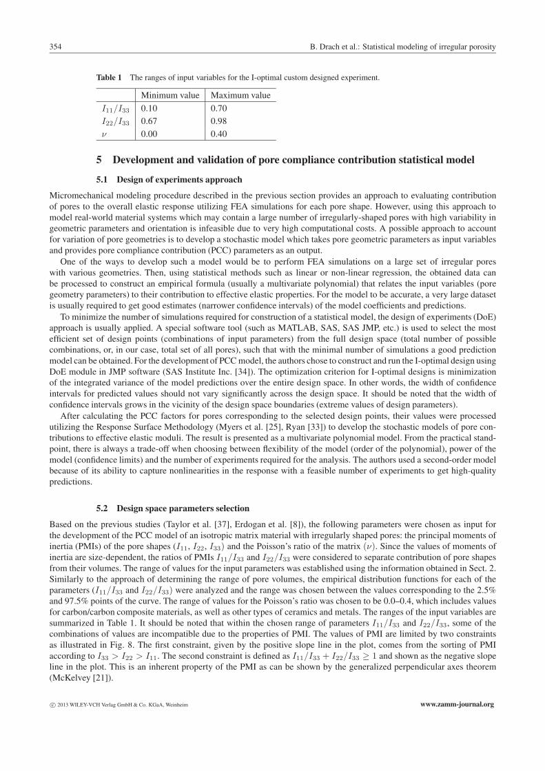
Table 1 The ranges of input variables for the I-optimal custom designed experiment.

Minimum value Maximum value

I11/I33 0.10 0.70

I22/I33 0.67 0.98

ν 0.00 0.40

5 Development and validation of pore compliance contribution statistical model

5.1 Design of experiments approach

Micromechanical modeling procedure described in the previous section provides an approach to evaluating contributionof pores to the overall elastic response utilizing FEA simulations for each pore shape. However, using this approach tomodel real-world material systems which may contain a large number of irregularly-shaped pores with high variability ingeometric parameters and orientation is infeasible due to very high computational costs. A possible approach to accountfor variation of pore geometries is to develop a stochastic model which takes pore geometric parameters as input variablesand provides pore compliance contribution (PCC) parameters as an output.

One of the ways to develop such a model would be to perform FEA simulations on a large set of irregular poreswith various geometries. Then, using statistical methods such as linear or non-linear regression, the obtained data canbe processed to construct an empirical formula (usually a multivariate polynomial) that relates the input variables (poregeometry parameters) to their contribution to effective elastic properties. For the model to be accurate, a very large datasetis usually required to get good estimates (narrower confidence intervals) of the model coefficients and predictions.

To minimize the number of simulations required for construction of a statistical model, the design of experiments (DoE)approach is usually applied. A special software tool (such as MATLAB, SAS, SAS JMP, etc.) is used to select the mostefficient set of design points (combinations of input parameters) from the full design space (total number of possiblecombinations, or, in our case, total set of all pores), such that with the minimal number of simulations a good predictionmodel can be obtained. For the development of PCC model, the authors chose to construct and run the I-optimal design usingDoE module in JMP software (SAS Institute Inc. [34]). The optimization criterion for I-optimal designs is minimizationof the integrated variance of the model predictions over the entire design space. In other words, the width of confidenceintervals for predicted values should not vary significantly across the design space. It should be noted that the width ofconfidence intervals grows in the vicinity of the design space boundaries (extreme values of design parameters).

After calculating the PCC factors for pores corresponding to the selected design points, their values were processedutilizing the Response Surface Methodology (Myers et al. [25], Ryan [33]) to develop the stochastic models of pore con-tributions to effective elastic moduli. The result is presented as a multivariate polynomial model. From the practical stand-point, there is always a trade-off when choosing between flexibility of the model (order of the polynomial), power of themodel (confidence limits) and the number of experiments required for the analysis. The authors used a second-order modelbecause of its ability to capture nonlinearities in the response with a feasible number of experiments to get high-qualitypredictions.

5.2 Design space parameters selection

Based on the previous studies (Taylor et al. [37], Erdogan et al. [8]), the following parameters were chosen as input forthe development of the PCC model of an isotropic matrix material with irregularly shaped pores: the principal moments ofinertia (PMIs) of the pore shapes (I11, I22, I33) and the Poisson’s ratio of the matrix (ν). Since the values of moments ofinertia are size-dependent, the ratios of PMIs I11/I33 and I22/I33 were considered to separate contribution of pore shapesfrom their volumes. The range of values for the input parameters was established using the information obtained in Sect. 2.Similarly to the approach of determining the range of pore volumes, the empirical distribution functions for each of theparameters (I11/I33 and I22/I33) were analyzed and the range was chosen between the values corresponding to the 2.5%and 97.5% points of the curve. The range of values for the Poisson’s ratio was chosen to be 0.0–0.4, which includes valuesfor carbon/carbon composite materials, as well as other types of ceramics and metals. The ranges of the input variables aresummarized in Table 1. It should be noted that within the chosen range of parameters I11/I33 and I22/I33, some of thecombinations of values are incompatible due to the properties of PMI. The values of PMI are limited by two constraintsas illustrated in Fig. 8. The first constraint, given by the positive slope line in the plot, comes from the sorting of PMIaccording to I33 > I22 > I11. The second constraint is defined as I11/I33 + I22/I33 ≥ 1 and shown as the negative slopeline in the plot. This is an inherent property of the PMI as can be shown by the generalized perpendicular axes theorem(McKelvey [21]).



Fig. 8 Design space for factors I11/I33, I22/I33.

To construct an I-optimal custom designed experiment, the following parameters were entered into the DoE module ofJMP software:

• Input variables (I11/I33, I22/I33, and ν) specified as continuous variables with ranges as shown in Table 1• Constraints for input variables: I22/I33 ≥ I11/I33, I11/I33 + I22/I33 ≥ 1• All model responses without optimization goals: E1, E2, E3, K, G• Prediction model type was set to the 2nd order Response Surface Model• Number of experimental runs (design points): 48• Number of center points: 5• Number of replicates: 0• Number of random starts for search of optimal designs: 1000

Note that the numbers of experimental runs and center points were chosen based on the analysis of the design evaluationparameters “Prediction Variance Profile”, “Prediction Variance Surface” and “Average Variance of Prediction” provided bythe JMP software. Center points are the experimental runs with all input variables set to the mean values of input ranges.These points are required for the 2nd order models to establish model curvature with respect to each of the input parameters(2nd order terms of the model).

The calculations resulted in a design table (see Table 2) containing combinations of input variables for each of theexperimental runs. Using this table, geometries with the desired values of I11/I33 and I22/I33 were selected from the totaldataset of pores obtained in Sect. 2. Since the number of pores in the dataset is finite, it was impossible to find pores withparameters that exactly match the values of the input parameters. Therefore, the pores with the smallest deviation fromthese values were chosen. Average differences between the actual and design parameters were −0.0008 and 0.0084 forI11/I33 and I22/I33, respectively. Root mean square errors (RMSE) were found to be 0.0307 for I11/I33, and 0.0325 forI22/I33.

Once the experimental pore set was selected and pore surface meshes were extracted using the procedure describedin Sect. 2, a self-written MATLAB script was employed to create FEA models for MSC Marc Mentat 2010 software(http://www.mscsoftware.com) and process the output files to determine pore compliance contribution parameters E1, E2,E3, K, G. For details on the FEA and post-processing procedures see (Drach et al. [7]).

5.3 3-factor designed experiment results

Results of the FEA simulations for the 3-factor designed experiment defined in Table 2 were processed and entered into theJMP software for statistical analysis. The “Fit Model” module was used with the following options:

• Standard least squares model• Response variables defined as: E1, E2, E3, K, G• Input variables I11/I33, I22/I33 and ν defined as the 2nd order “Response Surface Model Effects”



Table 2 Design table for the 3-factor designed experiment.

# I11/I33 I22/I33 ν # I11/I33 I22/I33 ν

1 0.100 0.900 0.2 28 0.435 0.837 0.2

2 0.100 0.900 0.4 29 0.435 0.825 0.2

3 0.100 0.900 0.4 30 0.451 0.825 0.4

4 0.100 0.980 0.0 31 0.456 0.825 0.2

5 0.100 0.980 0.0 32 0.458 0.825 0.2

6 0.100 0.980 0.2 33 0.460 0.825 0.2

7 0.100 0.980 0.4 34 0.461 0.825 0.2

8 0.169 0.831 0.0 35 0.461 0.870 0.0

9 0.169 0.831 0.0 36 0.464 0.825 0.4

10 0.169 0.831 0.2 37 0.468 0.825 0.2

11 0.330 0.670 0.0 38 0.469 0.825 0.0

12 0.330 0.670 0.0 39 0.471 0.825 0.2

13 0.330 0.670 0.2 40 0.700 0.825 0.2

14 0.330 0.670 0.2 41 0.700 0.670 0.0

15 0.330 0.670 0.4 42 0.700 0.670 0.0

16 0.330 0.670 0.4 43 0.700 0.670 0.2

17 0.340 0.980 0.4 44 0.700 0.670 0.4

18 0.373 0.980 0.2 45 0.700 0.670 0.4

19 0.383 0.980 0.2 46 0.700 0.814 0.2

20 0.400 0.980 0.0 47 0.700 0.825 0.0

21 0.400 0.980 0.2 48 0.700 0.825 0.4

22 0.400 0.980 0.4 49 0.700 0.980 0.0

23 0.433 0.825 0.2 50 0.700 0.980 0.0

24 0.435 0.837 0.2 51 0.700 0.980 0.2

25 0.435 0.837 0.2 52 0.700 0.980 0.4

26 0.435 0.837 0.2 53 0.700 0.980 0.4

27 0.435 0.837 0.2

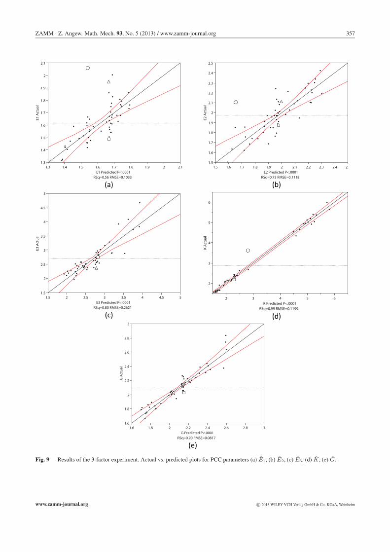
The results of the statistical analysis are presented in Fig. 9 as plots of actual vs predicted values. In these plots, thestraight line represents the perfect fit when the predicted values coincide with the actual values (Actual = Predicted).The two curves below and above straight line represent the confidence intervals for the predicted values. After visualinspection, the outlier data point shown as an empty circle in the graph was removed and the model was rerun to improvethe accuracy of predictions. Then the parameter estimates for each of the responses were inspected to determine which ofthe parameters were statistically significant. In the present study, the authors used the significance level of 90% as a criticalvalue. Insignificant parameters were excluded sequentially by removing one insignificant estimate at a time and re-runningthe model. It should be noted that exclusion of model effects obeys hierarchy of input variables in such a way that if asecond-order effect or one of the interactions of a specific input variable is significant but the input variable by itself isdetermined as insignificant, it cannot be excluded from the analysis. Plots shown in Fig. 9 represent model predictions withexcluded statistically insignificant model effects.

Accuracy of the model predictions was characterized using two indicators, R2 and RMSE. For the ideal model (perfectcorrelation with the experiment), R2 = 1 and RMSE = 0. In contrast, for an inadequate model, points on the plot willbe randomly scattered with no trend or a trend different from Actual = Predicted (R2 → 0, RMSE � 0). In an effortto improve accuracy of the proposed PCC model, visual analysis of the actual vs. predicted plot (Fig. 9) was performedfor each of the estimated responses. It was observed that in the midranges for responses E1, E2, E3, there is a significantnumber of points which fall beyond the confidence intervals. These points correspond to pores with very similar predictedresponse, but different values of the actual response.

An example of two pores with virtually the same predicted response and input parameters I11/I33, I22/I33, and νis shown in Fig. 10. Pore “a” is indicated on the plots (Fig. 9) as an empty square, and pore “b” as an empty triangle.



(a) (b)

(c) (d)

(e)

1.3

1.4

1.5

1.6

1.7

1.8

1.9

2

2.1

E1 A

ctua

l

1.3 1.4 1.5 1.6 1.7 1.8 1.9 2 2.1E1 Predicted P<.0001

RSq=0.56 RMSE=0.1033

1.5

1.6

1.7

1.8

1.9

2

2.1

2.2

2.3

2.4

2.5

E2 A

ctua

l

1.5 1.6 1.7 1.8 1.9 2 2.1 2.2 2.3 2.4 2.5E2 Predicted P<.0001

RSq=0.73 RMSE=0.1118

1.5

2

2.5

3

3.5

4

4.5

5

E3 A

ctua

l

1.5 2 2.5 3 3.5 4 4.5 5E3 Predicted P<.0001

RSq=0.80 RMSE=0.2621

2

3

4

5

6K

Act

ual

2 3 4 5 6K Predicted P<.0001

RSq=0.99 RMSE=0.1199

1.6

1.8

2

2.2

2.4

2.6

2.8

3

G A

ctua

l

1.6 1.8 2 2.2 2.4 2.6 2.8 3G Predicted P<.0001

RSq=0.90 RMSE=0.0817

Fig. 9 Results of the 3-factor experiment. Actual vs. predicted plots for PCC parameters (a) E1, (b) E2, (c) E3, (d) K , (e) G.



Comparing the shape features of these two pores, it appears that pore “b” has more surface features and looks less convexthan pore “a”. One of the ways to account for this difference would be to introduce in the model a non-dimensionalsurface area to volume ratio SV = S1/2/V 1/3, which is analogous to one of the shape coefficients in Rauch et al. [31] orthe sphericity parameter defined by Wadell as π1/3 (6V )2/3/S (Wadell [41]). The range of values for SV parameter waschosen using the same approach as for pore volumes and moments of inertia. The empirical distribution function for SV

was analyzed and the range was chosen between the values corresponding to the 2.5% and 97.5% points of the curve (seeTable 3).

Table 3 The ranges of input variables for the 4-factor designed experiment.

InputVariable

Minimumvalue

Maximumvalue

Average value(AVG)

Midrange value(MID)

I11/I33 0.10 0.70 0.40 0.30

I22/I33 0.67 0.98 0.825 0.155

SV 2.30 3.30 2.80 0.50

ν 0.00 0.40 0.20 0.20

Fig. 10 Two pores with very close geometric parameters I22/I11, I33/I11, but noticeably different mechanical response.

5.4 4-factor designed experiment results

For the development of a PCC model incorporating the SV factor, the authors constructed a new 4-factor experimentaldesign using the DoE module of JMP software with the following parameters:

• Input variables (I11/I33, I22/I33, ν and SV ) specified as continuous variables with ranges as shown in Table 3• Constraints for input variables: I22/I33 ≥ I11/I33, I11/I33 + I22/I33 ≥ 1• All model responses without optimization goals: E1, E2, E3, K, G• Prediction model type was set to the 2nd order Response Surface Model• Number of experimental runs (design points): 145• Number of center points: 5• Number of replicates: 0• Number of random starts for search of optimal designs: 1000

The design space of the experiment is presented in Table 4. Similarly to the previous design, it was impossible to find poreswith exactly matching parameters, and pores with the smallest deviations in parameters were selected. Average deviationsof the design parameters were −0.0039 for I11/I33, 0.0071 for I22/I33 and 0.0129 for SV . The root mean square errors(RMSE) were calculated as 0.0516, 0.0619, and 0.1562 for I11/I33, I22/I33 and SV , respectively.



Table 4 Designtableforthe4-factordesignedexperiment.

# I11I33

I22I33

SV ν # I11I33

I22I33

SV ν # I11I33

I22I33

SV ν

1 0.100 0.900 2.300 0.0 51 0.330 0.670 3.100 0.4 101 0.486 0.825 2.800 0.42 0.100 0.900 2.300 0.2 52 0.399 0.825 2.800 0.0 102 0.494 0.825 2.800 0.23 0.100 0.900 2.300 0.4 53 0.400 0.980 2.300 0.0 103 0.501 0.825 2.800 0.24 0.100 0.900 2.800 0.0 54 0.400 0.980 2.300 0.0 104 0.502 0.825 2.800 0.05 0.100 0.900 2.800 0.4 55 0.400 0.980 2.300 0.4 105 0.523 0.825 2.300 0.06 0.100 0.900 3.100 0.4 56 0.400 0.980 2.300 0.4 106 0.700 0.670 2.300 0.07 0.100 0.900 3.100 0.2 57 0.400 0.980 2.800 0.0 107 0.700 0.670 2.300 0.08 0.100 0.980 2.300 0.0 58 0.400 0.980 2.800 0.0 108 0.700 0.670 2.300 0.09 0.100 0.980 2.300 0.0 59 0.400 0.980 2.800 0.2 109 0.700 0.670 2.300 0.210 0.100 0.980 2.300 0.0 60 0.400 0.980 2.800 0.2 110 0.700 0.670 2.300 0.411 0.100 0.980 2.300 0.4 61 0.400 0.980 2.800 0.2 111 0.700 0.670 2.300 0.412 0.100 0.980 2.300 0.4 62 0.400 0.980 2.800 0.2 112 0.700 0.670 2.300 0.413 0.100 0.980 2.300 0.4 63 0.400 0.980 2.800 0.2 113 0.700 0.670 2.800 0.014 0.100 0.980 2.800 0.2 64 0.400 0.980 2.800 0.2 114 0.700 0.670 2.800 0.215 0.100 0.980 2.800 0.4 65 0.400 0.980 2.800 0.4 115 0.700 0.670 2.800 0.216 0.100 0.980 2.800 0.2 66 0.400 0.980 3.100 0.0 116 0.700 0.670 2.800 0.417 0.100 0.980 3.100 0.0 67 0.400 0.980 3.100 0.2 117 0.700 0.670 3.100 0.018 0.100 0.980 3.100 0.0 68 0.400 0.980 3.100 0.4 118 0.700 0.670 3.100 0.019 0.100 0.980 3.100 0.0 69 0.400 0.980 3.100 0.4 119 0.700 0.670 3.100 0.220 0.100 0.980 3.100 0.2 70 0.418 0.853 2.300 0.2 120 0.700 0.670 3.100 0.221 0.100 0.980 3.100 0.4 71 0.420 0.849 3.100 0.2 121 0.700 0.670 3.100 0.222 0.100 0.980 3.100 0.4 72 0.423 0.845 2.800 0.2 122 0.700 0.670 3.100 0.423 0.169 0.831 2.300 0.2 73 0.426 0.828 3.100 0.2 123 0.700 0.670 3.100 0.424 0.169 0.831 2.300 0.2 74 0.428 0.855 2.800 0.2 124 0.700 0.818 2.800 0.425 0.169 0.831 2.800 0.0 75 0.431 0.828 3.100 0.2 125 0.700 0.825 2.300 0.026 0.169 0.831 2.800 0.0 76 0.432 0.854 2.800 0.2 126 0.700 0.825 2.300 0.227 0.169 0.831 2.800 0.2 77 0.435 0.838 2.800 0.2 127 0.700 0.825 2.300 0.428 0.169 0.831 3.100 0.0 78 0.435 0.838 2.800 0.2 128 0.700 0.825 2.800 0.029 0.169 0.831 3.100 0.2 79 0.435 0.838 2.800 0.2 129 0.700 0.825 2.800 0.030 0.169 0.831 3.100 0.4 80 0.435 0.838 2.800 0.2 130 0.700 0.825 2.800 0.031 0.192 0.808 2.800 0.2 81 0.435 0.838 2.800 0.2 131 0.700 0.825 2.800 0.232 0.192 0.808 2.800 0.4 82 0.440 0.825 2.300 0.4 132 0.700 0.825 2.800 0.433 0.192 0.808 2.800 0.2 83 0.441 0.825 2.300 0.2 133 0.700 0.825 3.100 0.234 0.330 0.670 2.300 0.0 84 0.456 0.825 2.300 0.2 134 0.700 0.825 3.100 0.435 0.330 0.670 2.300 0.4 85 0.456 0.825 3.100 0.0 135 0.700 0.980 2.300 0.036 0.330 0.670 2.300 0.4 86 0.457 0.825 2.300 0.4 136 0.700 0.980 2.300 0.037 0.330 0.670 2.300 0.0 87 0.461 0.835 2.800 0.2 137 0.700 0.980 2.300 0.238 0.330 0.670 2.300 0.0 88 0.462 0.825 2.800 0.2 138 0.700 0.980 2.300 0.239 0.330 0.670 2.300 0.2 89 0.462 0.825 2.800 0.2 139 0.700 0.980 2.300 0.240 0.330 0.670 2.300 0.2 90 0.462 0.825 2.800 0.2 140 0.700 0.980 2.300 0.441 0.330 0.670 2.800 0.0 91 0.462 0.825 2.800 0.4 141 0.700 0.980 2.300 0.442 0.330 0.670 2.800 0.2 92 0.462 0.825 3.100 0.4 142 0.700 0.980 2.800 0.243 0.330 0.670 2.800 0.2 93 0.463 0.825 2.800 0.2 143 0.700 0.980 2.800 0.444 0.330 0.670 2.800 0.4 94 0.471 0.825 2.800 0.2 144 0.700 0.980 3.100 0.045 0.330 0.670 2.800 0.4 95 0.473 0.825 3.100 0.2 145 0.700 0.980 3.100 0.046 0.330 0.670 3.100 0.4 96 0.475 0.825 2.800 0.2 146 0.700 0.980 3.100 0.047 0.330 0.670 3.100 0.0 97 0.480 0.825 2.800 0.2 147 0.700 0.980 3.100 0.048 0.330 0.670 3.100 0.0 98 0.482 0.825 3.100 0.0 148 0.700 0.980 3.100 0.449 0.330 0.670 3.100 0.0 99 0.484 0.825 2.800 0.2 149 0.700 0.980 3.100 0.450 0.330 0.670 3.100 0.4 100 0.485 0.825 2.800 0.2 150 0.700 0.980 3.100 0.4



Once the experimental pore set was selected and pore surface meshes were extracted, FEA simulations were performedfor all pores and the results were imported into JMP software. The following options were selected in the “Fit Model”analysis module:

• Standard least squares model• Response variables defined as: E1, E2, E3, K, G• Input variables I11/I33, I22/I33, SV and ν defined as the 2nd order “Response Surface Model Effects”

The results of statistical modeling are presented in Fig. 11. It can be seen that the overall fit of the 4-factor model isbetter than that of the 3-factor model. This is evidenced by the increased values of R2 shown in Table 5. The scatterhas not changed significantly (similar RMSE values) for all model responses except K, for which an increased scatterwas observed. Also, due to the larger number of experimental runs, the new model has narrower confidence intervals forpredicted values of pore compliance contribution parameters. Goodness of fit (R2 and RMSE values) for both models issummarized in Table 5.

Table 5 Accuracy of model predictions of 3-factor and 4-factor PCC models.

Model response3-factor PCC model 4-factor PCC model

R2 RMSE R2 RMSE

E1 0.56 0.10 0.87 0.08

E2 0.73 0.11 0.75 0.11

E3 0.80 0.26 0.82 0.28

K 0.99 0.12 0.98 0.21

G 0.90 0.08 0.92 0.08

Table 6 Parameter estimates for 5 responses (contributions to elastic moduli) of the 4-factor PCC model. Standard errors are given inparentheses.

Coeff. Term E1 E2 E3 K G

α0 Intercept 1.673 (0.013) 1.997 (0.018) 3.077 (0.033) 2.484 (0.030) 2.226 (0.011)

α1 I11 0.466 (0.020) 0.291 (0.026) −1.122 (0.074) −0.487 (0.051) −0.155 (0.015)

α2 I22 0.161 (0.017) 0.405 (0.023) −0.857 (0.064) −0.349 (0.043) −0.107 (0.014)

α3 SV 0.242 (0.014) 0.125 (0.018) 0.265 (0.053) 0.339 (0.034) 0.200 (0.013)

α4 ν 0.010 (0.009) −0.008 (0.012) −0.174 (0.033) 1.884 (0.024) −0.274 (0.009)

α5 I211 −0.089 (0.023) −0.207 (0.031) 0.369 (0.101) 0.215 (0.057) 0

α6 I11I22 −0.212 (0.028) −0.267 (0.038) 0.859 (0.096) 0.502 (0.064) 0.120 (0.019)

α7 I222 −0.072 (0.022) 0.053 (0.029) 0 0 0

α8 I11SV 0 0 −0.212 (0.083) 0 −0.074 (0.017)

α9 I22SV 0 0 0 0 0

α10 S2V −0.118 (0.026) −0.125 (0.036) 0 0 0

α11 I11ν 0 0 0.101 (0.056) −0.155 (0.041) 0.044 (0.015)

α12 I22ν 0 0 0.105 (0.058) −0.125 (0.043) 0.037 (0.016)

α13 SV ν 0 0 −0.111 (0.054) 0.273 (0.040) −0.060 (0.015)

α14 ν2 −0.062 (0.014) −0.097 (0.019) 0 1.199 (0.035) −0.025 (0.013)

The parameter estimates of the 4-factor PCC model are presented in Table 6. These parameters are coefficients in thepolynomial model predicting dependence of pore contributions to elastic properties on the chosen geometric factors:

PCC = α0 + α1I11 + α2I22 + α3SV + α4ν + α5I211 + α6I11I22 + α7I

222 + α8I11SV + α9I22SV

+ α10S2V + α11I11ν + α12I22ν + α13SV ν + α14ν

2, (15)



where PCC is one of the following parameters E1, E2, E3, K or G characterizing pore contribution to effective Young’smoduli, bulk modulus and shear modulus; and the input factors are normalized to the range [−1; 1] based on the valuesprovided in Table 3:

I11 =I11/I33 − AV G (I11/I33)

MID (I11/I33), I22 =

I22/I33 − AV G (I22/I33)MID (I22/I33)

, (16)

SV =SV − AV G (SV )

MID (SV ), ν =

ν − AV G (ν)MID (ν)

.

5.5 Validation of the 4-factor PCC model and its comparison with approximationof pore shapes by ellipsoids

For validation of the proposed stochastic 4-factor PCC model, the authors compared the model estimates to the direct FEAsimulations on a new set of 150 pores which were not used for the model construction. Pore geometries were selected fromthe original dataset with all available pores. For this experiment, the design space was constructed using uniform distributionof the input variables within the boundaries given in Table 3. The results are shown in Fig. 12. For all five responses, themodel shows good prediction characterized by the low bias and moderate scatter (Table 7, the first two columns). It can beobserved that RMSE values for all responses are similar to those obtained for the original dataset. Low mean error (ME)and moderate RMSE values allow to conclude that the model is satisfactory for the new dataset.

In another study, the accuracy of approximations of pore shapes by ellipsoids was evaluated by comparing their responsewith direct FEA calculations for the materials with irregular shapes. Approximation of irregular shapes by ellipsoids wasperformed based on the values of principal moments of inertia and volumes as suggested, for example, in Borbely et al. [4]and Erdogan et al. [8]. Assuming mass density equal to unity, the expressions for the ellipsoids’ semi-axes are:

a =

√52

I22 + I33 − I11

V, b =

√52

I33 + I11 − I22

V, c =

√52

I11 + I22 − I33

V, (17)

where I11, I22, I33 are the principal moments of inertia of the considered pore (see Sect. 2), and V is the volume ofthe pore. The semi-axis a is aligned with the principal direction 1, b with direction 2, and c with direction 3. The porecompliance contribution parameters for ellipsoids were calculated using Eshelby solutions (Eshelby [10, 11]) as describedin Kachanov et al. [18], and formulas presented in Sect. 4.

The results of the comparison are presented in Fig. 13. It can be observed that the method of approximating ellipsoidsshows larger scatter and higher bias than the proposed PCC approach (Table 7). Thus, for the considered dataset, approxi-mation of irregular shapes by ellipsoids based on the principal moments of inertia produces less accurate predictions thanutilization of the proposed 4-factor PCC model. Note that approximations by ellipsoids seem to underpredict values of E1,E2, and K, which means that material with irregularly shaped pores will have lower values of the corresponding elasticparameters E1, E2, and K (see Eq. (13)) as compared to the material with ellipsoidal pores.

6 Conclusions

Processing of μCT data on porosity in C/C shows that orientation of pores can be characterized by directions of theirprincipal axes of inertia. As can be seen in Fig. 7, the pore orientation distributions are highly dependent on the morphologyof carbon fiber preform.

Contribution of pores to the effective elastic properties can be estimated using a stochastic model based on their geomet-ric parameters including ratios of their principal moments of inertia (I11/I33, I22/I33). Analysis shows that an improvedaccuracy can be achieved by incorporating a non-dimensionalized surface-to-volume ratio (SV ) as one of the model inputvariables.

The major result of this work is the 4-factor pore compliance contribution model given by Eq. (14) and Table 6. For thedataset of pores considered in this paper, the model provides better predictions of the material’s effective elastic propertiesthan the approach based on approximation of pore shapes by ellipsoids, as can be seen in Fig. 12, Fig. 13, and Table 7. Thepotential improvements of the model can be achieved by identifying other statistically significant factors which characterizepore shapes and their distribution.



(a) (b)

(c) (d)

(e)

1.2

1.3

1.4

1.5

1.6

1.7

1.8

1.9

2

2.1

2.2

2.3

E1 A

ctua

l

1.2 1.3 1.4 1.5 1.6 1.7 1.8 1.9 2 2.1 2.2 2.3E1 Predicted P<.0001

RSq=0.87 RMSE=0.0805

1.4

1.5

1.6

1.7

1.8

1.9

2

2.1

2.2

2.3

2.4

2.5

E2 A

ctua

l

1.4 1.5 1.6 1.7 1.8 1.9 2 2.1 2.2 2.3 2.4 2.5E2 Predicted P<.0001

RSq=0.75 RMSE=0.1084

1.5

2

2.5

3

3.5

4

4.5

5

5.5

6

E3 A

ctua

l

1.5 2 2.5 3 3.5 4 4.5 5 5.5 6E3 Predicted P<.0001

RSq=0.82 RMSE=0.2836

1

2

3

4

5

6

7

8

K A

ctua

l

1 2 3 4 5 6 7 8K Predicted P<.0001

RSq=0.98 RMSE=0.2086

1.6

1.8

2

2.2

2.4

2.6

2.8

3

3.2

G A

ctua

l

1.6 1.8 2 2.2 2.4 2.6 2.8 3 3.2G Predicted P<.0001

RSq=0.92 RMSE=0.0765

Fig. 11 Results of the 4-factor experiment. Actual vs. predicted plots for PCC parameters (a) E1, (b) E2, (c) E3, (d) K, (e) G.



(a) (b)

(c) (d)

(e)

1.2

1.4

1.6

1.8

2

2.2

2.4

2.6

1.2 1.4 1.6 1.8 2 2.2 2.4 2.6

E1 A

ctua

l

E1 PredictedME = -0.0607, RMSE = 0.1389

1.6

1.8

2

2.2

2.4

2.6

2.8

1.6 1.8 2 2.2 2.4 2.6 2.8

E2 A

ctua

l

E2 PredictedME = -0.0614, RMSE = 0.1579

1.6

2

2.4

2.8

3.2

3.6

4

4.4

4.8

5.2

1.6 2 2.4 2.8 3.2 3.6 4 4.4 4.8 5.2

E3 A

ctua

l

E3 PredictedME = 0.0536, RMSE = 0.3106

1.2

1.8

2.4

3

3.6

4.2

4.8

5.4

6

1.2 1.8 2.4 3 3.6 4.2 4.8 5.4 6

K Ac

tual

K PredictedME = 0.0831, RMSE = 0.3014

1.7

1.9

2.1

2.3

2.5

2.7

2.9

1.7 1.9 2.1 2.3 2.5 2.7 2.9

G Ac

tual

G PredictedME = -0.0242, RMSE = 0.0814

Fig. 12 Results of the validation study of the 4-factor experiment. Actual vs. predicted plots for PCC parameters (a) E1, (b) E2, (c)E3, (d) K, (e) G.



(a) (b)

(c) (d)

(e)

1.1

1.3

1.5

1.7

1.9

2.1

2.3

2.5

1.1 1.3 1.5 1.7 1.9 2.1 2.3 2.5

E1 A

ctua

l

E1 EllipsoidsME = -0.2817, RMSE = 0.3425

1.4

1.6

1.8

2

2.2

2.4

2.6

2.8

1.4 1.6 1.8 2 2.2 2.4 2.6 2.8

E2 A

ctua

l

E2 EllipsoidsME = -0.1460, RMSE = 0.2348

2

2.4

2.8

3.2

3.6

4

4.4

4.8

5.2

5.6

6

6.4

6.8

2 2.4 2.8 3.2 3.6 4 4.4 4.8 5.2 5.6 6 6.4 6.8

E3 A

ctua

l

E3 EllipsoidsME = 0.2790, RMSE = 0.5016

1.4

2

2.6

3.2

3.8

4.4

5

5.6

1.4 2 2.6 3.2 3.8 4.4 5 5.6

K Ac

tual

K EllipsoidsME = -0.1612, RMSE = 0.3010

1.6

1.8

2

2.2

2.4

2.6

2.8

3

1.6 1.8 2 2.2 2.4 2.6 2.8 3

G Ac

tual

G EllipsoidsME = -0.0455, RMSE = 0.1578

Fig. 13 Comparison of the pore approximations by ellipsoids with FEA calculations for actual shapes. Actual vs. predicted plots forPCC parameters (a) E1, (b) E2, (c) E3, (d) K , (e) G.



Acknowledgements The authors gratefully acknowledge the financial support of the National Science Foundation (NSF) and GermanScience Foundation (DFG) through the grant DMR-0806906 “Materials World Network: Multi-Scale Study of Chemical Vapor InfiltratedCarbon/Carbon Composites”. Igor Tsukrov also acknowledges the US Fulbright Senior Scholar Award.

The microtomography data was provided by Stefan Dietrich, Jorg-Martin Gebert, and Romana Piat from Karlsruhe Institute of Tech-nology (KIT, Germany). Fruitful discussions of C/C characterization and modeling techniques with Thomas Bohlke, Romana Piat, BorisReznik (KIT), and Todd Gross from the University of New Hampshire (UNH) are greatly appreciated. The authors also express theirgratitude to Philip Ramsey (UNH) for valuable discussions on statistical analysis and design of experiment methodologies.

References

[1] Y. Benveniste, A new approach to the application of Mori-Tanaka’s theory in composite materials, Mech. Mater. 6, 147–157(1987).

[2] W. Benzinger and K. J. Huttinger, Chemistry and kinetics of chemical vapor infiltration of pyrocarbon-V. Infiltration of carbonfiber felt, Carbon 37, 941–946 (1999).

[3] J. Blow and A. J. Binstock, How to find the inertia tensor (or other mass properties) of a 3D solid body represented by a trianglemesh., http://number-none.com/blow/inertia/bb inertia.doc (Retrieved July 25, 2011) (2004).

[4] A. Borbely, F. F. Csikor, S. Zabler, P. Cloetens, and H. Biermann, Three-dimensional characterization of the microstructure of ametal–matrix composite by holotomography, Mater. Sci. Eng. A 367, 40–50 (2004).

[5] T. Bohlke, K. Jochen, R. Piat, T. Langhoff, I. Tsukrov, and B. Reznik, Elastic properties of pyrolytic carbon with axisymmetrictextures. Tech. Mech. 30, 343–353 (2010).

[6] E. C. David and R. W. Zimmerman, Compressibility and shear compliance of spheroidal pores: Exact derivation via the Eshelbytensor, and asymptotic expressions in limiting cases, Int. J. Solids Struct. 48, 680–686 (2011).

[7] B. Drach, I. Tsukrov, T. Gross, S. Dietrich, K. Weidenmann, R. Piat, and T. Bohlke, Numerical modeling of carbon/carboncomposites with nanotextured matrix and 3D pores of irregular shapes, Int. J. Solids Struct. 48, 2447–2457 (2011).

[8] S. T. Erdogan, E. J. Garboczi, and D. W. Fowler, Shape and size of microfine aggregates: X-ray microcomputed tomography vs.laser diffraction, Powder Technol. 177, 53–63 (2007).

[9] O. Eroshkin and I. Tsukrov, On micromechanical modeling of particulate composites with inclusions of various shapes, Int. J.Solids Struct. 42, 409–427 (2005).

[10] J. D. Eshelby, The determination of the elastic field of an ellipsoidal inclusion, and related problems, edited by A. Nur, Proc. R.Soc. A Math. Phys. Eng. Sci. 241, 376–396 (1957).

[11] J. D. Eshelby, The elastic field outside an ellipsoidal inclusion, Proc. R. Soc. Lond. Ser. A Math. Phys. Sci. 252, 561–569 (1959).[12] E. J. Garboczi, Three dimensional shape analysis of JSC-1A simulated lunar regolith particles, Powder Technol. 207, 96–103

(2011).[13] J.-M. Gebert, A. Wanner, R. Piat, M. Guichard, S. Rieck, B. Paluszynski, and T. Bohlke, Application of the micro-computed

tomography for analyses of the mechanical behavior of brittle porous materials, Mech. Adv. Mater. Struct. 15, 467–473 (2008).[14] T. Gross, K. Nguyen, M. Buck, N. Timoshchuk, I. Tsukrov, B. Reznik, R. Piat, and T. Bohlke, Tension–compression anisotropy

of in-plane elastic modulus for pyrolytic carbon, Carbon 49, 2145–2147 (2011).[15] Z. Hashin, Thermoelastic properties and conductivity of carbon/carbon fiber composites, Mech. Mater. 8, 293–308 (1990).[16] R. Hill, Elastic properties of reinforced solids: Some theoretical principles, J. Mech. Phys. Solids 11, 357–372 (1963).[17] I. T. Jolliffe, Principal Component Analysis, second edition, edited by K. Diamantaras and S. Kung (Springer, New York, 2002).[18] M. Kachanov, B. Shafiro, and I. Tsukrov, Handbook of Elasticity Solutions (Kluwer Academic Publishers, Dordrecht, 2003).[19] M. Kachanov, I. Tsukrov, and B. Shafiro, Effective moduli of solids with cavities of various shapes. Appl. Mech. Rev. 47, 151

(1994).[20] A. Li, S. Zhang, B. Reznik, S. Lichtenberg, G. Schoch, and O. Deutschmann, Chemistry and kinetics of chemical vapor deposition

of pyrolytic carbon from ethanol, Proc. Combust. Inst. 33, 1843–1850 (2011).[21] J. P. McKelvey, A generalization of the perpendicular axis theorem for the rotational inertia of rigid bodies, Am. J. Phys. 51, 658

(1983).[22] N. Michailidis, F. Stergioudi, H. Omar, and D. Tsipas, FEM modeling of the response of porous Al in compression, Comput.

Mater. Sci. 48, 282–286 (2010).[23] T. Mori and K. Tanaka, Average stress in matrix and average elastic energy of materials with misfitting inclusions, Acta Metallur-

gica 21, 571–574 (1973).[24] T. Mura, Micromechanics of Defects in Solids, 2nd rev ed. (Kluwer Academic Publishers, Dordrecht, 1987).[25] R. H. Myers, D. C. Montgomery, and C. M. Anderson-Cook, Response Surface Methodology: Process and Product Optimization

Using Designed Experiments, third edition (John Wiley and Sons, Hoboken, NJ, 2009).[26] S. Nemat-Nasser and M. Hori, Micromechanics: Overall Properties of Heterogeneous Solids, 2nd edition (Elsevier Science Pub-

lishers, Amsterdam, 1999).[27] D. H. Pahr and P. K. Zysset, From high-resolution CT data to finite element models: development of an integrated modular frame-

work, Comput. Methods Biomech. Biomed. Eng. 12, 45–57 (2009).[28] H. E. Pettermann, H. J. Bohm, and F. G. Rammerstorfer, Some direction-dependent properties of matrix-inclusion type composites

with given reinforcement orientation distributions, Compos. Part B, Eng. 28, 253–265 (1997).



[29] R. Piat, I. Tsukrov, N. Mladenov, M. Guellali, R. Ermel, T. Beck, E. Schnack, and M. J. Hoffmann, Material modeling of theCVI-infiltrated carbon felt II. Statistical study of the microstructure, numerical analysis and experimental validation, Compos.Sci. Technol. 66, 2769–2775 (2006).

[30] R. Piat, I. Tsukrov, N. Mladenov, V. Verijenko, M. Guellali, E. Schnack, M. J. Hoffmann, Material modeling of the CVI-infiltratedcarbon felt I: Basic formulae, theory and numerical experiments, Compos. Sci. Technol. 66, 2997–3003 (2006).

[31] L. Rauch, M. Pernach, K. Bzowski, and M. Pietrzyk, On application of shape coefficients to creation of the statistically similarrepresentative element of DP steels. Submitted (2012).

[32] B. Reznik and K. J. Huttinger, On the terminology for pyrolytic carbon, Carbon 40, 621–624 (2002).[33] T. P. Ryan, Modern Experimental Design (John Wiley & Sons, Hoboken, NJ, 2007).[34] SAS Institute Inc., 2010. JMP 9 Design of Experiments Guide. SAS Institute Inc, Cary, NC, www.jmp.com/support/downloads/-

pdf/jmp902/doe guide.pdf (Retrieved September 28, 2011).[35] I. Sevostianov and M. Kachanov, Explicit cross-property correlations for anisotropic two-phase composite materials, J. Mech.

Phys. Solids 50, 253–282 (2002).[36] I. Sevostianov, M. Kachanov, and T. I. Zohdi, On computation of the compliance and stiffness contribution tensors of non ellip-

soidal inhomogeneities, Int. J. Solids Struct. 45, 4375–4383 (2008).[37] M. Taylor, E. J. Garboczi, S. T. Erdogan, and D. W. Fowler, Some properties of irregular 3-D particles, Powder Technol. 162, 1–15

(2006).[38] B. Tomkova, M. Sejnoha, J. Novak, and J. Zeman, Evaluation of Effective Thermal Conductivities of Porous Textile Composites,

Int. J. Multiscale Comput. Eng. 6, 153–167 (2008).[39] I. Tsukrov and B. Drach, Elastic deformation of composite cylinders with cylindrically orthotropic layers, Int. J. Solids Struct.

47, 25–33 (2010).[40] I. Tsukrov and J. Novak, Effective elastic properties of solids with defects of irregular shapes, Int. J. Solids Struct. 39, 1539–1555

(2002).[41] H. Wadell, Volume, Shape and roundness of quartz particles, J. Geol. 43, 250–280 (1935).[42] C. Zhang and T. Chen, Efficient Feature Extraction for 2D/3D Objects in Mesh Representation. In: Proceedings of the 2001

International Conference on Image Processing, Vol. 3, (IEEE, 2001), pp. 935–938.


characterization and statistical modeling of irregular porosity in

Documents