characterization of (co)polymers by maldi-tof-mscharacterization of (co)polymers by maldi-tof-ms...
TRANSCRIPT

Characterization of (co)polymers by MALDI-TOF-MS
Citation for published version (APA):Staal, B. B. P. (2005). Characterization of (co)polymers by MALDI-TOF-MS. Eindhoven: Technische UniversiteitEindhoven. https://doi.org/10.6100/IR583506
DOI:10.6100/IR583506
Document status and date:Published: 01/01/2005
Document Version:Publisher’s PDF, also known as Version of Record (includes final page, issue and volume numbers)
Please check the document version of this publication:
• A submitted manuscript is the version of the article upon submission and before peer-review. There can beimportant differences between the submitted version and the official published version of record. Peopleinterested in the research are advised to contact the author for the final version of the publication, or visit theDOI to the publisher's website.• The final author version and the galley proof are versions of the publication after peer review.• The final published version features the final layout of the paper including the volume, issue and pagenumbers.Link to publication
General rightsCopyright and moral rights for the publications made accessible in the public portal are retained by the authors and/or other copyright ownersand it is a condition of accessing publications that users recognise and abide by the legal requirements associated with these rights.
• Users may download and print one copy of any publication from the public portal for the purpose of private study or research. • You may not further distribute the material or use it for any profit-making activity or commercial gain • You may freely distribute the URL identifying the publication in the public portal.
If the publication is distributed under the terms of Article 25fa of the Dutch Copyright Act, indicated by the “Taverne” license above, pleasefollow below link for the End User Agreement:www.tue.nl/taverne
Take down policyIf you believe that this document breaches copyright please contact us at:[email protected] details and we will investigate your claim.
Download date: 26. Jun. 2020

Characterization of (co)polymers by MALDI-TOF-MS
Bastiaan Staal

Cover: The enclosure of a (co)polymer MALDI-TOF-MS spectrum into the polymer characteristics can be seen as a challenging jigsaw. The colored spot on the front cover represents a gradient copolymer fingerprint as described in chapter 6. The figure at the back side represents the coupling between SEC-MALDI visualized as a SEC chromatogram which is connected to a MALDI spectrum.

Characterization of (co)polymers by MALDI-TOF-MS
PROEFSCHRIFT
ter verkrijging van de graad van doctor aan de Technische Universiteit Eindhoven, op gezag van de
Rector Magnificus, prof.dr. R.A. van Santen, voor een commissie aangewezen door het College voor
Promoties in het openbaar te verdedigen op dinsdag 18 januari 2005 om 16.00 uur
door
Bastiaan Bram Pieter Staal
geboren te Hoogerheide

Dit proefschrift is goedgekeurd door de promotoren: prof.dr. A.M. van Herk en prof.dr.ir. P.J. Schoenmakers CIP-DATA LIBRARY TECHNISCHE UNIVERSITEIT EINDHOVEN Staal, Bastiaan B.P. Characterization of (co)polymers by MALDI-TOF-MS / door Bastiaan Bram Pieter Staal. – Eindhoven : Technische Universiteit Eindhoven, 2005. Proefschrift. - ISBN 90-386-2826-9 NUR 913 Subject headings: polymer and copolymer characterization; fingerprints / mass spectrometry; MALDI-TOF / size exclusion chromatography; SEC / discriminant analysis / molecular weight distribution / light scattering / viscosity Trefwoorden: polymeer- en copolymeerkarakterisatie; vingerafdruk / massaspectroscopie; MALDI-TOF / exclusiechromatografie; SEC / discriminatie-analyse / molmassaverdeling / lichtverstrooiing / viscositeit © 2004, Bastiaan Staal Printed by Printpartners Ipskamp te Endschede An electronic copy of this thesis is avaiable from the site of the Eindhoven University Library in PDF format (http://w3.tue.nl/nl/diensten/bib).

Opgedragen aan mijn ouders


Table of contents
1 General introduction ..........................................................................................................11 1.1 Introduction........................................................................................................................11 1.2 Outline of this thesis. .........................................................................................................12
2 Matrix Assisted Laser Desorption/Ionization Time of Flight Mass Spectrometry (MALDI-TOF-MS) ........................................................................................15
2.1 Introduction........................................................................................................................15 2.2 Basic principles..................................................................................................................15
2.2.1 Transfer of polymer molecules into the gas phase.....................................................16 2.2.2 Separation of the polymer molecules.........................................................................17 2.2.3 Variations in flight time .............................................................................................19 2.2.4 Detection of the ions ..................................................................................................21
2.3 Experimental parameters ...................................................................................................21 2.3.1 Instrument settings .....................................................................................................22
2.4 Data analysis ......................................................................................................................23 2.5 Molar-mass distribution .....................................................................................................26
3 Absolute molar-mass distributions ...............................................................................31
3.1 Introduction........................................................................................................................31 3.2 Size-Exclusion Chromatography (SEC) ............................................................................32
3.2.1 Experimental ..............................................................................................................34 3.3 Calibration methods in SEC...............................................................................................34
Conventional calibration............................................................................................................35 Universal calibration..................................................................................................................36 Static light scattering..................................................................................................................39 Calibration of detector constants ...............................................................................................40
3.4 Band broadening in SEC....................................................................................................42 3.5 Results................................................................................................................................43
Error analysis .............................................................................................................................47 3.6 Conclusions........................................................................................................................49
4 The relationship between the MMD from MALDI and from SEC ...................59
4.1 Introduction........................................................................................................................59 4.2 Experimental ......................................................................................................................60 4.3 Results and discussion .......................................................................................................61
4.3.1 The relationship between the MMD from MALDI and from SEC ...........................61 4.4 SEC and MALDI-TOF-MS ...............................................................................................62 4.5 Conclusions........................................................................................................................68
5 MALDI of homopolymers ................................................................................................75
5.1 Introduction........................................................................................................................75 5.2 Definitions..........................................................................................................................75
5.2.1 Determination of numbers of repeat units and end-group masses .............................75 5.2.2 End-group Correlation Function (ECF) .....................................................................77 5.2.3 Auto-Correlation Function (ACF) .............................................................................80 5.2.4 Conclusion .................................................................................................................81
5.3 End-group analysis with MALDI-TOF-MS to reveal the initiator functionality ..............82 5.3.1 Introduction................................................................................................................82 5.3.2 The use of the ECF function ......................................................................................92
5.4 Copolymerizations of polyketones ....................................................................................94 5.4.1 Results and discussion ...............................................................................................96
6 MALDI of copolymers .....................................................................................................107 6.1 Introduction......................................................................................................................107 6.2 Copolymer analysis..........................................................................................................107
6.2.1 Copolymer topologies..............................................................................................108 6.2.2 Copolymer structure.................................................................................................109 6.2.3 Peak-shape differences.............................................................................................110 6.2.4 Overlapping isotopes ...............................................................................................110 6.2.5 Isotope broadening...................................................................................................114
6.3 Copolymer fingerprints ....................................................................................................114 6.3.1 Isotope overlap and isotope interference .................................................................114 6.3.2 Calculation of Anr∆ and Bnr∆ for isotope overlap ..................................................116 6.3.3 Calculation of Anr∆ and Bnr∆ for isotope interference ...........................................120 6.3.4 Estimating the chemical composition. .....................................................................122
6.4 characteristics of copolymer fingerprints.........................................................................125 6.4.1 Block copolymers ....................................................................................................125 6.4.2 Random copolymers ................................................................................................126
6.5 End-group analysis...........................................................................................................131 6.6 Determining types of topology ........................................................................................132 6.7 Polystyrene-co-isoprene...................................................................................................134 6.8 Polystyrene-gradient-butadiene .......................................................................................139
6.8.1 Experimental section................................................................................................139 6.8.2 MALDI-TOF-MS Analysis .....................................................................................139
6.9 Conclusions......................................................................................................................142 7 Outlook and development ..............................................................................................149 Glossary of Symbols and Abbreviations ..................................................................................151 Summary ..................................................................................................................................154 Samenvatting ............................................................................................................................156 Scientific papers .......................................................................................................................158 Acknowledgements ..................................................................................................................159 Curriculum vitae.......................................................................................................................160


General introduction 11
Chapter 1
1 General introduction
1.1 Introduction
The molecular characterization of polymeric material is a key step in elucidating the relationship
between polymer properties, morphology, and chemical structure. The challenge for polymer
chemists is to control and alter the polymerization conditions to obtain polymers with well-defined
molecular structures and desired properties. The research into and development of synthetic
polymers during the last century has led to new classes of polymers. The new types of synthetic
polymers, with tailor-made properties and often complex structures, e.g. gradient copolymer,
require better characterization techniques such as coupled (“hyphenated”) systems. Traditionally
characterization involves molar-mass analysis, repeat-unit or sequence analysis, end-group analysis,
and purity examination. The techniques used, such as light scattering, viscometry, NMR and FTIR
provide a wealth of information, albeit this information is only an average over the entire molar-
mass distribution. Size exclusion chromatography does characterize molar-mass distributions, but it
is a technique with many imperfections (see chapter 3). Mass spectrometry is an attractive
alternative for the molecular characterization of polymeric material. Due to its high sensitivity and
accuracy, a single measurement reveals nearly as much (and often more accurate) information as
most of the traditional characterization techniques together.
During the past decade, mass spectrometry has revolutionized the characterization of synthetic
polymers1. With the introduction of matrix-assisted-laser-desorption ionization time-of-flight mass
spectrometry (MALDI-TOF-MS), it has become possible to bring intact polymers in the gas phase
predominately singly charged, i.e. without degrading the polymer molecule. This so-called soft
ionization technique offers the possibility to obtain structural information on polymer chains as a

12 Chapter 1
function of its molar mass, i.e. repeat units, end-group masses, copolymer compositions and some
aspects of the polymer topology (see chapter 6) as well the overall molar mass distribution (MMD).
Mass spectrometry has many advantages over other polymer-characterization techniques, because it
measures the mass over charge ratio of ions, allowing individual polymer chains to be studied. Mass
spectrometry also has its limitations. For example, quantification is only possible to a limited
extent. Moreover, mass discrimination is a known phenomenon. Although various authors2-9 have
shown that accurate molar-mass distributions can be obtained for polymers with a low
polydispersity index (PDI<1.2 is a reasonable indication), for samples with a higher polydispersity,
both underestimation and overestimation of the high-molar-mass fractions have been reported10,11.
The complexity of the obtained spectra and the difficulty of interpretation, especially for copolymer
systems, is another issue with requires attention.
In this thesis MALDI-TOF-MS was extensively used to characterize (co)polymer systems in terms
of absolute molar masses, end groups, and the chain construction (number(s) of repeat units used to
construct a polymer chain). The chain construction provides direct information of the polymer
topology (block, random or gradient). Methods to elucidate polymer topology are often time
consuming, whereas MALDI is an accurate and fast characterization method. Special attention was
devoted to the development of new mathematical techniques to extract the embedded information
from complex spectra. Software was written to identify and characterize spectra exhaustively.
1.2 Outline of this thesis
MALDI-TOF-MS is an absolute method for molar-mass determination. However, as mentioned
before, mass discrimination affects the experimentally determined MMD. An alternative method to
determine the MMD is Size-Exclusion Chromatography (SEC). Chapter 3 describes different
calibration methods to obtain the molar mass distribution from SEC. Chapter 4 focuses on the
proper conversion of the MALDI-TOF-MS signal to a “SEC-like” signal and on the validation of
the conversion method. The second part of chapter 4 describes a quantitative study of mass
discrimination, by comparing molar-mass distributions of a broad mixture of polystyrenes obtained
by SEC and MALDI.
Chapter 5 deals with the development of new mathematical techniques for end-group analysis and
homopolymer analysis. The end-group-correlation function (ECF) rapidly reveals all possible end
groups present in the sample. The accuracy of the obtained end-group masses is not always
sufficient to decide between end groups of nearly the same mass. An expanded ECF method was
developed to exploit the maximum accuracy of a MALDI measurement. A recently published

General introduction 13
method, the autocorrelation function (ACF), can be used to obtain the repeat-mass units and a
possible identification of the polymer12.
In chapter 6 the more-challenging complex copolymer spectra are discussed. The numerous
possible combinations in which monomers are manifested in polymeric chains are beyond the limits
of one simple algorithm to extract all embedded characteristics of the copolymer from a mass
spectrum such as end groups, block-length distributions, chemical composition and the copolymer
topology. The methods, described in chapter 6, require an absolute minimum of prior knowledge
about the polymer sample. The relative abundance of the peaks in a spectrum is different for each
topology, which makes it possible to distinguish between, for example, a gradient and block
copolymer. Therefore one should not look at each peak individually, but at the coherence of all
peaks within the entire molar-mass distribution. The analysis of dozens of peaks is laborious and
calls for appropriate software. The methods described in chapter 6 form the basis of the software
developed in-house. With this software a full Molar-Mass-Chemical-Composition Distribution
(MMCCD), the polymer architecture, and the individual block-length distributions (i.e. the length
distributions of the A and B blocks) can be obtained from only one simple MALDI-TOF-MS
measurement. In the final chapter the status of MALDI-TOF-MS and future developments are
discussed.
14 Chapter 1
Reference List 1. Hanton, S. D. Chem. Rev. 2001, 101, 527-569.
2. Byrd, M. H. C.; McEwen, C. N. Anal. Chem. 2000, 72, 4568-4576.
3. Lehrle, R. S.; Sarson, D. S. Polym. Degrad. Stab. 1996, 51, 197-204.
4. Tang, X.; Dreifuss, P. A.; Vertes, A. Rapid Commun. Mass Spectrom. 1995, 9, 1141-1147.
5. Belu, A. M.; DeSimone, J. M.; Linton, R. W.; Lange, G. W.; Friedman, R. M. J. Am. Soc. Mass Spectrom. 1996, 7, 11-24.
6. Schriemer, D. C.; Li, L. Anal. Chem. 1997, 69, 4176-4183.
7. Shimada, K.; Lusenkova, M. A.; Sato, K.; Saito, T.; Matsuyama, S.; Nakahara, H.; Kinugasa, S. Rapid Commun. Mass Spectrom. 2001, 15, 277-282.
8. Rashidzadeh, H.; Guo, B. Anal. Chem. 1998, 70, 131-135.
9. Axelsson, J.; Scrivener, E.; Haddleton, D. M.; Derrick, P. J. Macromolecules 1996, 29, 8857-8882.
10. McEwen, C. N.; Jackson, C.; Larsen, B. S. Int. J. Mass Spectrom. Ion Phys 1997, 160, 387-394.
11. Hanton, S. D.; Clark, P. A.; Owens, K. G. J. Am. Soc. Mass Spectrom. 1999, 10, 104-111.
12. Wallace, W. E.; Guttman, C. M.; Antonucci, J. M. J. Am. Soc. Mass Spectrom. 1999, (10), 224-230.

MALDI-TOF-MS 15
Chapter 2
2 Matrix Assisted Laser Desorption/Ionization Time of Flight Mass Spectrometry (MALDI-TOF-MS)
2.1 Introduction
Traditionally, mass-spectrometry techniques based on magnetic and electrical fields, time-of-flight,
ion trap and ion cyclotron resonance, are the most commonly used techniques to separate ions by
their mass over charge ratio. Until recently, the most common ionization technique was electron
ionization. This technique is based on the electron irradiation of vaporized sample molecules,
resulting in ionized molecules and fragments. Since polymers are not volatile and fragmentation of
ionized polymers should be avoided, this technique is not suitable to obtain structural information
of complex mixtures of polymer molecules, with for example, a molar-mass distribution (MMD). A
more appropriate choice would be a mass spectrometry technique that place charged polymer
molecules in the gas phase without degrading the polymer sample.
In the last decade, soft ionization techniques such as matrix assisted laser desorption/ionization
(MALDI) and electrospray ionization (ESI) have enabled the introduction of intact high-molar-mass
polymers into the gas phase. The work described in this thesis is focused on MALDI. MALDI is
predominantly used for all but not the (very) nonpolar synthetic polymers , whereas ESI is generally
used for polar polymers. Note that for MALDI, synthetic polymers only form a small part of the
application field. A simple literature search on MALDI returns numerous articles on proteins and
other biopolymers, and only a few on synthetic polymers.
2.2 Basic principles
MALDI mass spectrometry may be regarded as a three-step process. The first step concerns the
production of charged gas-phase species from the original polymer molecules. This step involves

16 Chapter 2
the transfer of the solid material into the gas phase and its ionization. The second step involves the
separation of the ionized polymers according to mass or, more correctly, according to mass over
charge ratio (m/z). The last step involves the detection of the ions.
According to the IUPAC, the mass of molecular ion obtained by mass spectrometry is expressed in
amu, being the unified atomic mass unit based on the convention that the mass of the isotope 12C
equals 12 amu exactly.
The MALDI three-step process will be described in more detail in the next sections.
2.2.1 Transfer of polymer molecules into the gas phase
The MALDI process is the ablation of the polymer molecules dispersed in a matrix of small
organic-molecules, most commonly organic acids. In a typical MALDI experiment the polymer
molecules, the matrix, and optionally the salt of an organic acid are deposited together on a target
plate. A short ultraviolet or infrared laser pulse is fired at the deposited sample on the target. The
role of the matrix can be seen as mediator for energy absorption of the laser. The highly ultraviolet
absorbing matrix transfers the laser energy efficient and guards the polymer molecules from
excessive amounts of energy. The laser energy excites the matrix molecules, causing the matrix to
vaporize and decompose into what is called a supersonic phase transformation1. As a result of this
phase transformation a plume of matrix species and polymer species is spread into the gas phase.
In general, ions or exited species are formed by the removal or addition of an electron giving a
radical cation M+• or anion M-•, respectively, or by the addition of other charged species:
A + e-• → A+• + 2e-
or with a lower probability:
A + e- → A-•
A + e- → A*+ e-
A + X+ → [AX]+
Where X corresponds to proton, Na-, K- or Ag- etc. atom, A denotes the molecular species to be
ionized, e- an electron and * indicates an exited species.
Besides the polymer molecules, matrix molecules and cations, also clusters of polymer molecules,
matrix molecules, and cations have been detected in the plume2-4. Clusters of the polymer
molecules, can typically be seen at molar masses exceeding 10,000 amu.

MALDI-TOF-MS 17
Synthetic polymers are not easy to charge (negative or positive), unless they contain labile protons,
as for example in the case of polyacrylic acid. The majority of the synthetic polymers requires the
addition of a salt to the polymer-matrix mixture for effective adduction of ions to the polymer. For
rather polar polymers alkali-metal ions are normally used. Ions such as Na+ and K+ are often present
as impurities originating from the glassware or solvent used in the sample preparation, or are simply
present as impurity in the matrix material. For nonpolar polymers that contain double bonds, an
organic salt with Ag+ or Cu2+ is added.
Irrespective of the normally stable charged state of the metal ion, MALDI produces only single
charged polymeric species in the gas phase5. This behavior is still not completely understood.
Although the ionization mechanism is not completely understood, it was thought to be a
straightforward explanation that laser generated ions are formed by the direct multiphoton
ionization of a matrix molecule leading to a matrix radical cation. However, the ionization
potentials for matrix molecules in crystals or matrix aggregates are still not know. Moreover, other
experiments revealed that the potential energies are rather far too high to result in direct
multiphoton ionization. More details about the possible ionization steps has been given by Zenobi
and Knochenmuss6. The theory of Karas and Kruger7 claimed that the ionization process may be
understood as initial formation of clusters between matrix, analyte (and salt ions) which brake down
to singly charged species.
2.2.2 Separation of the polymer molecules
After the polymer molecules are transferred to the gas phase as an ion, the ionized polymers are
separated on the basis of mass over charge ratio (m/z). For MALDI, the most common mass-
separation technique is Time-of-Flight (TOF). Other mass separation techniques, such as
quadrupole-filter, Fourier-Transform Mass Spectroscopy (FTMS) and Ion Trap Spectroscopy (ITS)
can be used as well but are currently limited to masses up to m/z 4,000 and 20,000 respectively8,9.
In a TOF analyzer a high voltage (typically 25 kV over a distance of a few millimeters) accelerates
the ions from the MALDI plume. After the acceleration, the ions enter into an evacuated tube of
typically one meter long, the so-called drift tube. The obtained velocity is given by the simple
equation:
2
2νmVze =∆ (2.1)
Where V∆ is the electric potential difference applied to accelerate the ion with charge ez ⋅ , m the
mass of the charged (polymer) molecules, and ν the velocity. Since the drift tube is long compared
to the acceleration region, ν can be expressed as:
18 Chapter 2
0ttL−
=ν (2.2)
Where L is the length of the drift tube, 0t is the time when the ablating laser pulse hits the target,
and t is the total flight time of the ions. Substitution of (2.2) into (2.1) yields:
( )20
2
2 t tm e Vz L
−= ∆ or ( )20ttC
zm
−= (2.3)
Where C is a constant. This general calibration equation relates the mass-to-charge with the flight
time of the ions. Small corrections to this equation have been published elsewhere10,11.
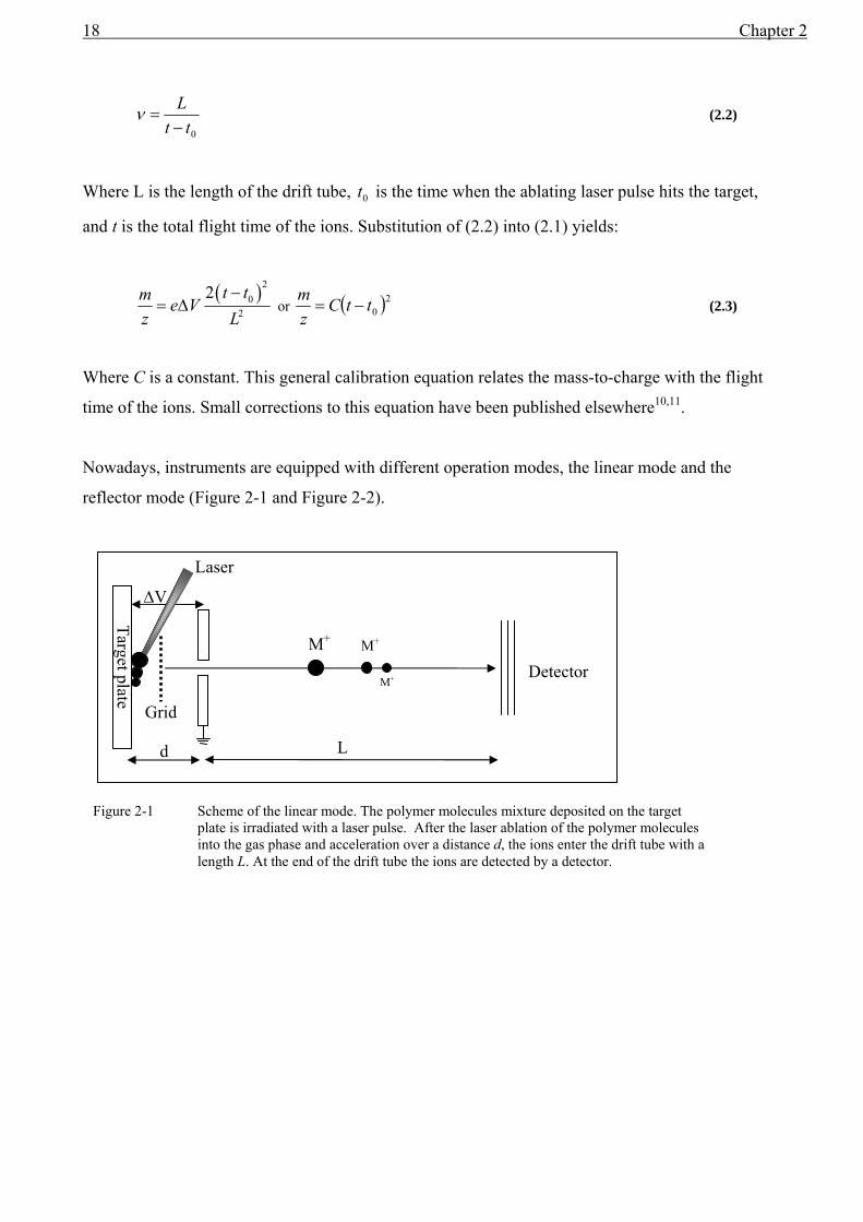
Nowadays, instruments are equipped with different operation modes, the linear mode and the
reflector mode (Figure 2-1 and Figure 2-2).
M+ M+
M+
L d
∆V
Detector
Laser
Figure 2-1 Scheme of the linear mode. The polymer molecules mixture deposited on the target plate is irradiated with a laser pulse. After the laser ablation of the polymer molecules into the gas phase and acceleration over a distance d, the ions enter the drift tube with a length L. At the end of the drift tube the ions are detected by a detector.
Target plate Grid

MALDI-TOF-MS 19
The main difference between the linear and the reflector mode is the electrical mirror which reflects
the ions. Ions of a given mass and velocity will penetrate into the field of the reflector to a different
content. Fast ions penetrate deeper into the field and, hence, take a longer time to be reflected. The
longer flight time will enhance the resolution.
The mass resolution in a time-of-flight system is given by11
2m tm t∆ ∆
= (2.4)
Where m∆ is the mass difference across a peak at full-width-half-height (FWHH), m the mass, t the
flight time and t∆ the time difference across a peak at FWHH.
According to Equation (2.3), m∆ is proportional to t L∆ . A longer flight tube will decrease the
value of m∆ and increase the resolution.
2.2.3 Variations in flight time
Variations in flight times, due to the initial-velocity distribution, finite sample-deposition height and
instability of the polymer molecules, are explained in Figure 2-3.
M+ M+
M+
L d
Detector
∆Vref
Reflector
Laser
∆V
Target plate
Figure 2-2 Scheme of the reflector mode. In contrast to the linear mode, ions are reflected at the end of the drift tube. An electrostatic-energy mirror provides a cascade of retarding fields in a direction opposite to the acceleration field. After reflection the ions hit the detector.
Grid

20 Chapter 2
The last situation in Figure 2-3 is an example of fragmentation. Fragmentation that takes place
during the ablation by the laser or during the acceleration is called early fragmentation12, prompt
fragmentation13.
An effective way to reduce the energy spread of the ions is delayed extraction. A second plate,
called grid (Figure 2-1 and Figure 2-2), placed a few millimeters from the target, is charged for a
brief time, keeping the plume trapped after the laser ablation. After the grid voltage is suddenly
switched to zero, potential ions with large initial-velocity vectors pointed towards the entrance of
the drift tube will experience a lower potential difference than ions with a small initial-velocity
vector. In other words, at the moment the grid voltage drops to zero, ions close to the target plate
will experience the maximum potential difference, resulting in a high velocity. Ions located further
away from the target surface will experience a lower potential difference, resulting in a lower
velocity. In this way ions with the same mass, but different velocities, will reach the detector at the
same time. This correction is dependent on molar mass and can only be applied across a certain
molar mass range.
The phenomenon that molecules fragment in the drift tube after acceleration is called late
fragmentation. Late fragmentation has no effect on the kinetic energy of the ions in the linear mode
and the ions will reach the detector at the correct time. However, in the reflector mode these ions
Two ions of the same mass, the same, but opposite-initial velocities and the same initial kinetic energy.
21 νν −= , tt 21 νν > , )0()0( 21 tt = Two ions of the same mass, the same initial velocity, and the same kinetic energy, but originated at different locations (thickness differences of the deposited sample) on the target. 21 νν = ,
tt 21 νν > , )0()0( 21 tt = Two ions of the same mass, the same initial velocity, and the same kinetic energy, but ionized at different times during the laser ablation of the matrix. 21 νν = , tt 21 νν = , )0()0( 21 tt ≠ Two ions of the same mass, a different initial velocity, and a different initial kinetic energy.
21 νν ≠ , tt 21 νν > , )0()0( 21 tt = One of the ions fragments in such a way that two of the remaining ions have the same mass. Initial kinetic energy is the same.
21 νν ≠ , tt 21 νν > , )0()0( 21 tt =
+
+
1ν 2ν
+ t1ν ∆V
+
+
1ν 2ν
+ t1ν
+ t2ν
+
+
1ν
2ν + t1ν
+ t2ν
+
+
1ν
2ν + t1ν
+
+
1ν + t1ν t2ν
+ t2ν
+ t2ν
+ + 2ν
target
Entrance of the drift tube Figure 2-3 Illustration of the variations in flight time due to the different events at the onset of the ionization
process.

MALDI-TOF-MS 21
are re-accelerated with the mass of the charged fragment and will reach the detector at the incorrect
times. Late fragmentation12 or also called post-scource decay can be used to perform MS-MS
experiments to obtain molecular information. Unfortunately this technique is strongly dependent of
the stability of the polymer in the gas phase and not frequently used due to much better alternatives
to perform MS-MS experiments, e.g. quadrupole-filter and collision induced MALDI.
2.2.4 Detection of the ions
The MultiChannel Plate (MCP) is the most common detector used for polymers. The MCP consists
of an assembly of lead and glass capillaries, coated on the inside with electron-emissive materials,
and fused together. The capillaries are biased by a high voltage. Ions strike the inside wall, creating
secondary electrons which amplifies each ion-impact signal. The secondary electrons are measured
by photo multiplication. MCP detectors tend to saturate easily and may also be less sensitive for
high-molar-mass molecules, since the ion-to-electron conversion is dependent on the impact
velocity14,15.
2.3 Experimental parameters
The methods for sample preparation described in literature are numerous and seem to have a
somewhat alchemistic touch. However, only two processes in sample preparation dominate the
quality of spectra: the co-crystallization and the homogeneous mixing of matrix and sample. As a
rule of thumb, the polarity of the matrix and the polymer should be similar, so that both are soluble
in a common solvent. In this way the intimate mixing of matrix, polymer molecules, and salt will
result in the best co-mixing of the deposited solid mixture.
The most commonly used methods for sample preparation are hand-spotting and sample spraying.
The hand-spotted or dry-droplet method uses a pipette to deposit 0.3-2 µL of the matrix, polymer
molecules, and salt solution on the target. The solvent will evaporate and matrix crystals are usually
obtained. The main disadvantage of the hand-spotting method is the large signal variation across the
target plate. A more homogeneous co-crystallization of the matrix and sample is obtained by
electrospray deposition or by air-spray deposition. The majority of the work in this thesis is done by
the hand-spotted method.
In this work, one matrix is used extensively: trans-2-[3-(4-tert-Butylphenyl)-2-methyl-2-
propenylidene]malononitrile (DCTB)a. Besides the low threshold for the laser energy, this matrix
a This matrix is now commercially available. The synthesis of the matrix DCTB used in this thesis is described elsewhere16
22 Chapter 2
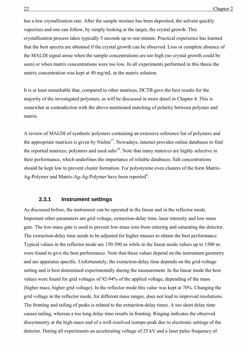
has a low crystallization rate. After the sample mixture has been deposited, the solvent quickly
vaporizes and one can follow, by simply looking at the target, the crystal growth. This
crystallization process takes typically 5 seconds up to one minute. Practical experience has learned
that the best spectra are obtained if the crystal growth can be observed. Loss or complete absence of
the MALDI signal arose when the sample concentrations are too high (no crystal growth could be
seen) or when matrix concentrations were too low. In all experiments performed in this thesis the
matrix concentration was kept at 40 mg/mL in the matrix solution.
It is at least remarkable that, compared to other matrices, DCTB gave the best results for the
majority of the investigated polymers, as will be discussed in more detail in Chapter 4. This is
somewhat in contradiction with the above-mentioned matching of polarity between polymer and
matrix.
A review of MALDI of synthetic polymers containing an extensive reference list of polymers and
the appropriate matrices is given by Nielen17. Nowadays, internet provides online databases to find
the reported matrices, polymers and used salts18. Note that many matrices are highly selective in
their performance, which underlines the importance of reliable databases. Salt concentrations
should be kept low to prevent cluster formation. For polystyrene even clusters of the form Matrix-
Ag-Polymer and Matrix-Ag-Ag-Polymer have been reported4.
2.3.1 Instrument settings
As discussed before, the instrument can be operated in the linear and in the reflector mode.
Important other parameters are grid voltage, extraction-delay time, laser intensity and low-mass
gate. The low-mass gate is used to prevent low-mass ions from entering and saturating the detector.
The extraction-delay time needs to be adjusted for higher masses to obtain the best performance.
Typical values in the reflector mode are 150-500 ns while in the linear mode values up to 1500 ns
were found to give the best performance. Note that these values depend on the instrument geometry
and are apparatus specific. Unfortunately, the extraction-delay time depends on the grid-voltage
setting and is best determined experimentally during the measurement. In the linear mode the best
values were found for grid voltages of 92-94% of the applied voltage, depending of the mass
(higher mass, higher grid voltage). In the reflector mode this value was kept at 70%. Changing the
grid voltage in the reflector mode, for different mass ranges, does not lead to improved resolutions.
The fronting and tailing of peaks is related to the extraction-delay times. A too short delay time
causes tailing, whereas a too long delay time results in fronting. Ringing indicates the observed
dissymmetry at the high-mass end of a well-resolved isotope-peak due to electronic settings of the
detector. During all experiments an accelerating voltage of 25 kV and a laser pulse frequency of

MALDI-TOF-MS 23
20Hz were applied. The laser used is most commonly a 337nm wavelength nitrogen laser. The
laser energy per unit area is adjustable. Under normal conditions, the laser energy is adjusted to the
minimum intensity to avoid fragmentation. Low laser energy results in a low initial velocity and a
narrow initial-velocity distribution within the plume7. A narrow initial-velocity distribution
minimizes the variations in flight time.
2.4 Data analysis
The mass-axis calibration is normally performed by using a (bio)polymer with known end groups.
In case of a protein, only one signal is obtained. Using a synthetic polymer allows calibration of the
entire mass range at once. To obtain the best calibration, the same matrix is used at a position, on
the target, close (or the same) to the calibration spot. A position far away from the calibration
position is more often biased due to imperfections of the target-surface flatness.
More challenging is the calibration of the signal axis, as this axis may be in error due to a variety of
reasons19. Moments of the molar-mass distribution as determined by MALDI-TOF-MS are often
lower than those determined via classical methods.15,20-23 This is generally attributed to mass
discrimination. Mass discrimination could originate from: (1) Desorption difference. The fact that
desorption of low-molar-mass species is more promoted than that of high molar mass species. No
evidence for this effect has been provided so far. (2) Detector saturation, due to the slow charge-up
recovery of the MCP detectors15,24,25. (3) The way the ions are detected. For high-molar-mass
species the ion-to-ion conversion is diminished due to the decrease of the ion impact velocity14,15.
(4) The data handling such as raw data transformation and baseline corrections.
Mass discrimination as given by the first three items can be diminished using samples with narrow
molar mass distributions. To prevent mass discrimination as given by the fourth item will be
discussed in the following text.
Improper transformation of the raw data signal, e.g. conversion of the time domain to the mass
domain, leads to erroneous molar-mass distributions. Furthermore, baselines drawn in MALDI
TOF-MS require a multi-point line which could lead to errors.
24 Chapter 2
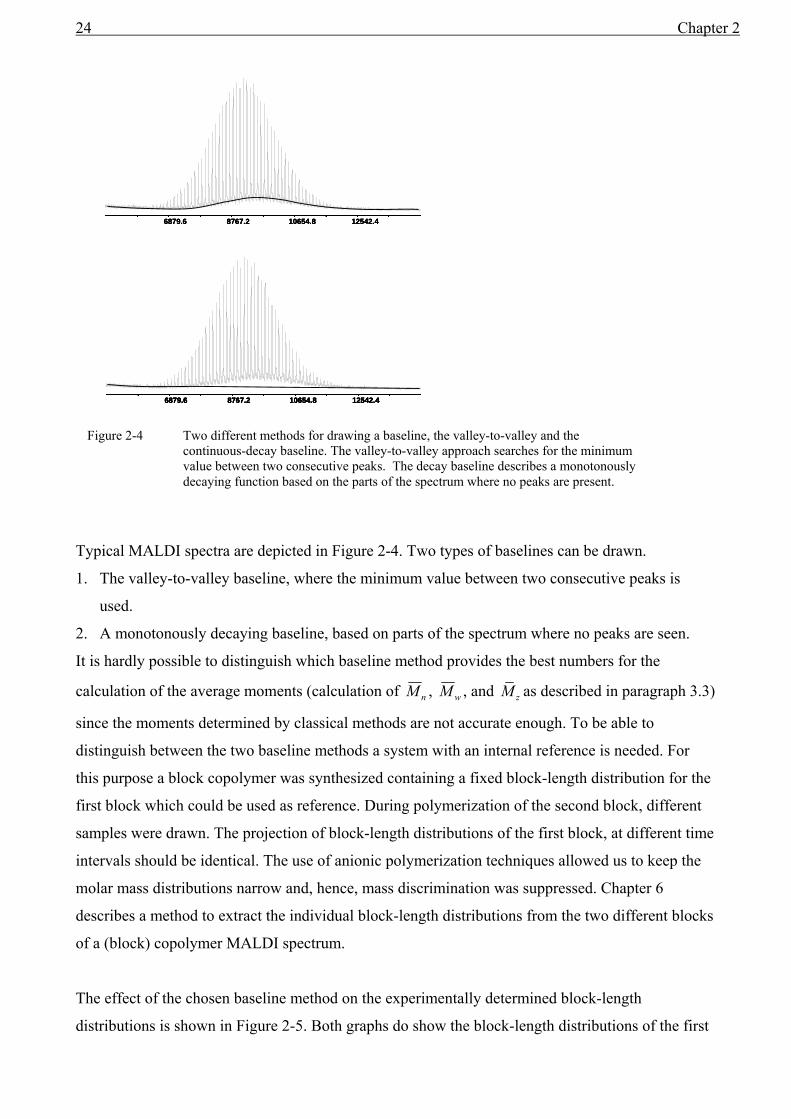
Typical MALDI spectra are depicted in Figure 2-4. Two types of baselines can be drawn.
1. The valley-to-valley baseline, where the minimum value between two consecutive peaks is
used.
2. A monotonously decaying baseline, based on parts of the spectrum where no peaks are seen.
It is hardly possible to distinguish which baseline method provides the best numbers for the
calculation of the average moments (calculation of nM , wM , and zM as described in paragraph 3.3)
since the moments determined by classical methods are not accurate enough. To be able to
distinguish between the two baseline methods a system with an internal reference is needed. For
this purpose a block copolymer was synthesized containing a fixed block-length distribution for the
first block which could be used as reference. During polymerization of the second block, different
samples were drawn. The projection of block-length distributions of the first block, at different time
intervals should be identical. The use of anionic polymerization techniques allowed us to keep the
molar mass distributions narrow and, hence, mass discrimination was suppressed. Chapter 6
describes a method to extract the individual block-length distributions from the two different blocks
of a (block) copolymer MALDI spectrum.
The effect of the chosen baseline method on the experimentally determined block-length
distributions is shown in Figure 2-5. Both graphs do show the block-length distributions of the first
6879.6 8767.2 10654.8 12542.4
6879.6 8767.2 10654.8 12542.4
6879.6 8767.2 10654.8 12542.46879.6 8767.2 10654.8 12542.4
6879.6 8767.2 10654.8 12542.46879.6 8767.2 10654.8 12542.46879.6 8767.2 10654.8 12542.4
Figure 2-4 Two different methods for drawing a baseline, the valley-to-valley and the continuous-decay baseline. The valley-to-valley approach searches for the minimum value between two consecutive peaks. The decay baseline describes a monotonously decaying function based on the parts of the spectrum where no peaks are present.

MALDI-TOF-MS 25
block, obtained from different samples drawn during the synthesis of the second block. For
completeness the homopolymer of the starting block is included. Although the block length of the
first block is fixed, a slight change in block length maximum is observed. The spectra in the upper
graph were corrected with the monotonously-decaying-function method. The spectra in the bottom
graph are corrected with the valley-to-valley baseline method. A significant improvement has been
realized in the overlaid distributions. All peaks display the maximum intensity at the same chain
length. The valley-to-valley baseline method shows the best performance and will be used in this
thesis for baseline corrections. Unfortunately, this method can only work if all peaks of interest are
well separated. As soon as peaks start to overlap, the entire baseline rises. As a rule of thumb,
masses below 25,000 amu can be corrected with the valley-to-valley method. Masses exceeding
25,000 amu must be corrected by fitting a monotonously decaying function. Note that molar masses
exceeding 25,000 amu are generally not sensitive to the baseline settings.

26 Chapter 2
2.5 Molar-mass distribution
The MCP detector counts the number of ions that hit the detector plate. The intensity in MALDI
reflects the total number of counted ions of a given mass. Therefore, MALDI measures the number
molar-mass distribution nMMD. The transformation of the MALDI signal from the time domain to
the mass domain is different for each instrument26. The instrument used in this thesis records all
data in the time domain and converts the data directly to the mass domain using equation 2.3. This
is not completely correct. The area of a time interval dtt + represents a certain number of species
with a given singly charged mass dmm + . Whether the integration takes place in the time domain
or mass domain, the number of species remains the same. The area A can be written as:
5 10 15 20 25 30 35 40
0.00
0.02
0.04
0.06
0.08
0.10
Inte
nsity
(a.u
.)
Number of repeat units
sample 1 sample 2 sample 3 sample 4 Homopolymer
5 10 15 20 25 30 35 40
0.00
0.02
0.04
0.06
0.08
0.10
Inte
nsity
(a.u
.)
Number of repeat units
sample 1 sample 2 sample 3 sample 4 Homopolymer
Figure 2-5 Observed block length distributions of the same spectra, but with different baseline-corrections methods.
Valley-to-valley method
Monotonously-decaying-function method
MALDI-TOF-MS 27
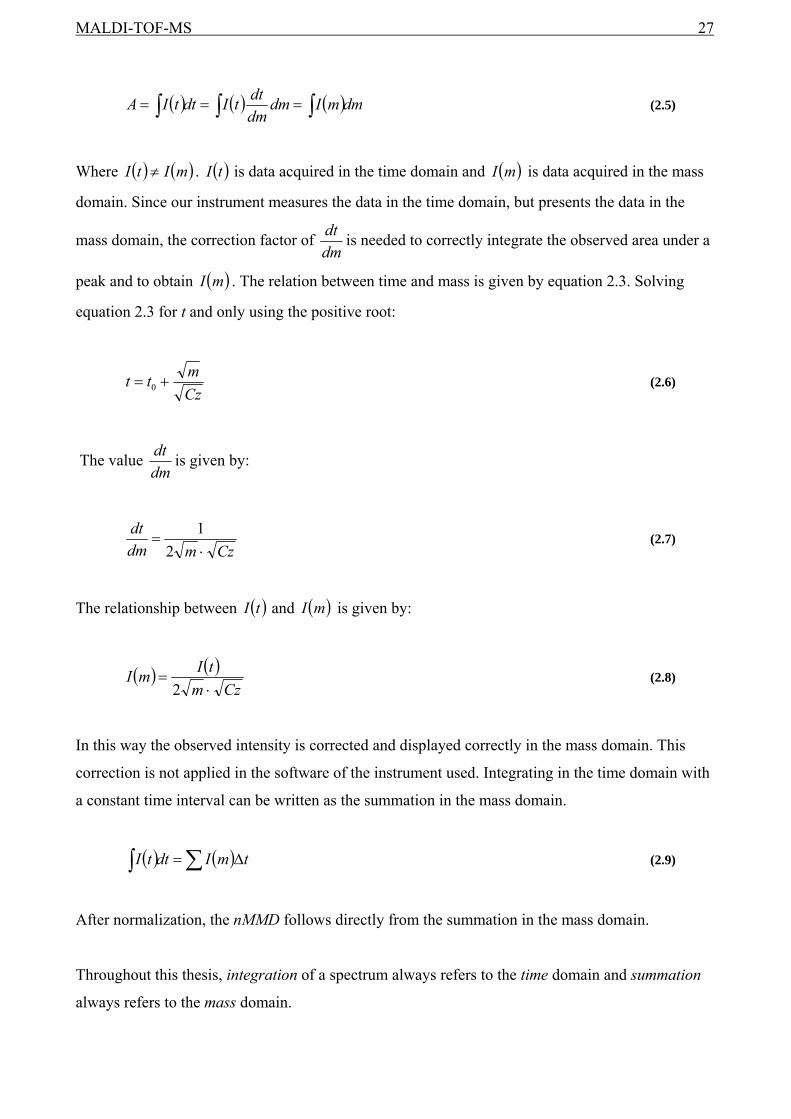
( ) ( ) ( )dmmIdmdmdttIdttIA ∫∫∫ === (2.5)
Where ( ) ( )mItI ≠ . ( )tI is data acquired in the time domain and ( )mI is data acquired in the mass
domain. Since our instrument measures the data in the time domain, but presents the data in the
mass domain, the correction factor of dmdt is needed to correctly integrate the observed area under a
peak and to obtain ( )mI . The relation between time and mass is given by equation 2.3. Solving
equation 2.3 for t and only using the positive root:
Czmtt += 0 (2.6)
The value dmdt is given by:
Czmdmdt
⋅=
21
(2.7)
The relationship between ( )tI and ( )mI is given by:
( ) ( )Czm
tImI⋅
=2
(2.8)
In this way the observed intensity is corrected and displayed correctly in the mass domain. This
correction is not applied in the software of the instrument used. Integrating in the time domain with
a constant time interval can be written as the summation in the mass domain.
( ) ( )∑∫ ∆= tmIdttI (2.9)
After normalization, the nMMD follows directly from the summation in the mass domain.
Throughout this thesis, integration of a spectrum always refers to the time domain and summation
always refers to the mass domain.

28 Chapter 2
For synthetic polymers, it is of utmost importance to obtain a good representation of the MMD
obtained by MALDI to compare it with the MMD obtained by the classical polymer
characterization methods, such as SEC. Mass discrimination can be prevented if the samples are
narrowly distributed in terms of mass. SEC offers an excellent opportunity to split a broad MMD
into narrow fractions and, hence, the combination of SEC and MALDI is an attractive approach.
The quantitative aspects of mass discrimination, as well the comparison between the MMD from
MALDI and from SEC are discussed in Chapter 4.

MALDI-TOF-MS 29
Reference List 1. Vertes, A.; Irinyi, G.; Gijbels, R. Anal. Chem. 1993, 65, 2389-2393.
2. Knochenmuss, R.; Lehmann, E.; Zenobi, R. European Journal of Mass Spectrometry 1998, 4, 421-426.
3. Rashidzadeh, H.; Guo, B. J. Am. Soc. Mass Spectrom. 1998, 9, 724-730.
4. Goldschmidt, R. J.; Guttman, C. M. J. Am. Soc. Mass Spectrom. 2000, 11 (1095), 1106.
5. Karas, M.; Gluckmann, M.; chaefer, J. J. Mass Spectrom. 2000, 35, 1-12.
6. Zenobi, R.; Knochenmuss, R. Mass Spectrom Rev. 1998, 17, 337.
7. Karas, M.; Krüger, R. Chem. Rev. 2003, 103, 427-439.
8. Siuzdak, G. Mass Spectromerty for Biotechnology, Academic Press, San Diego, 1996.
9. Watson, J. L. Introduction to Mass spectrometry, Lippencott-Raven, New York, 1997, 3rd ed.
10. Juhasz, P.; Vestal, M. L.; Martin, S. A. J. Am. Soc. Mass Spectrom. 1997, 8, 209-217.
11. Cotter, R. J. Time-of-Flight Mass Spectrometry, American Chemical Society, Washington, D.C., 1997.
12. Guttman, C. M. MS, John Wiley & Sons, Inc., New York, 2002.
13. Patterson, S. D.; Katta, V. Anal. Chem. 1994, 66, 3121-3132.
14. Geno, P. W.; Macfarlane, R. D. Int. J. Mass Spectrom. Ion Processes 1989, 92, 195-210.
15. Schriemer, D. C.; Li, L. Anal. Chem. 1997, 69, 4169-4175.
16. Ulmer, L.; Mattay, J.; Torres-Garcia, H. G.; Luftmann, H. European Journal of Mass Spectrometry 2000, 6 (1), 49-52.
17. Nielen, M. W. F. Mass Spectrom Rev. 1999, 18, 309-344.
18. . http://polymers.msel.nist.gov/maldirecipes.
19. Zhu, H. H.; Yalcin, T.; Li, L. J. Am. Soc. Mass Spectrom. 1998, 9, 275-281.
20. Larsen, B. S.; Simonsick, W. J.; McEwen, C. N. J. Am. Soc. Mass Spectrom. 1996, 7, 287-292.
21. Lehrle, R. S.; Sarson, D. S. Rapid commun. Mass Spectrom. 1995, 9, 91-92.
22. Montaudo, G.; Montaudo, M.S.; Puglisi, C.; Samperi, F. Rapid commun. in Mass Spectrom. 1995, 9, 453-460.
23. Guttman, C. M.; Wetzel, J.W.; Wallace, W.E.; Blair, W.R.; Goldschmidt, R.M.; Vanderhart, D.L.; Fanconi, B.M.; . Polym. Prepr. 2000, 41, 678-679.

30 Chapter 2
24. Westman, A.; Brinkmalm, G.; Barofsky, D. F. Int. J. Mass Spectrom. Ion Processes 1997, 169/170, 79-97.
25. McEwen, C. N.; Jackson, C.; Larsen, B. S. Int. J. Mass Spectrom. Ion Phys 1997, 160, 387-394.
26. Guttman, C. M. Polym. Prepr. 1996, 37, 837-838.

Absolute molar-mass distributions 31
Chapter 3
3 Absolute molar-mass distributions
3.1 Introduction
The molar mass (M) and the molar-mass distribution (MMD) of polymers are perhaps the most
important characteristics for establishing of structure-property relationships for (end product)
processing performance. Such relationships are needed not only for the development of new
products, but also for quality control and improving existing materials.
Size-exclusion chromatography (SEC), also called gel-permeation chromatography, is the most
widely used method to determine the molar mass and the MMD.
During the past several years there have been significant advances in SEC column technology,
detection systems, and new applications. Combinations of SEC with molar-mass sensitive detectors
are used to determine the absolute MMD, while the hyphenation of SEC with other techniques,
specifically mass spectrometry, gives rise to accurate and detailed information. The latter
hyphenation technique constitutes a two-dimensional separation, which can help us understand
complex relationships between, for example, MMD and the chemical composition distribution
(CCD).
SEC and MALDI can be used to obtain the MMD. Since SEC is a well-established method for
determining the MMD and MALDI is a relative new method, an attempt has been made to compare
the MMD obtained by both methods.
In SEC, light-scattering detectors are claimed to measure the absolute MMD, although many
parameters need to be calibrated, which may contribute to an erroneous MMD. In this chapter
different methods of detection and calibration methods for obtaining the absolute MMD are
discussed.

32 Chapter 3
3.2 Size-Exclusion Chromatography (SEC)
SEC belongs to the family of liquid chromatography separation techniques. It separates molecules
based on molecular size or, more precisely, based on hydrodynamic volume. In a typical SEC setup
a column packed with porous material is flushed with a constant flow of a mobile phase. When a
polymer sample is injected into the system and passes through the column, very large molecules
will not penetrate into the pores of the packing and will elute first. Smaller molecules, which can
penetrate into the pores, will elute at a later time. The sample is separated or fractionated according
to molecular size.
The molecules which are too large to penetrate the pores of the column packing elute within the
interstitial or exclusion volume exV , which is the volume of mobile phase between the packing
particles. In contrast, molecules smaller than the smallest pore sizes diffuse freely into the pores and
have full access to the total permeation volume or total pore volume pV .
The chromatographic behavior of analytes separated by SEC can be described by the generic SEC
equation1:
pSECexret VKVV ⋅+= (3.1)
where SECK is the distribution coefficient, relating the average concentration of the analyte in the
pore volume to that in the excluded volume. Two limiting cases can be distinguished: 1=SECK , the
molecules can completely enter all the pores and elute at the permeation limit of the column, and
0=SECK , when none of the molecules can enter the pores and they elute at the total exclusion limit.
Molecules that can enter parts of the pore volume are in the region where 10 << SECK . In this
region molecules are separated according to their size. More practically, columns are characterized
by the molar-mass range where 10 << SECK . Therefore the exclusion limit and the permeation
limit are expressed in terms of molar mass (most commonly of polystyrene in tetrahydrofuran
(THF)). Calibration standards are normally used to obtain the relationship between molar mass and
retention time.
Well-defined standards of known molar masses are used to construct the calibration curve. Note
that this calibration is only valid for polymers of the same type and chemical structure. After the
calibration curve has been constructed, the molar-mass distribution can be calculated if we assume
the detector response to be linearly proportional to the concentration and the separation to be strictly
according to molar mass. The relationship between the weight fraction belonging to a specific molar
mass between M and dMM + and the normalized detector response w from retention volume v
to dvv + is2:
Absolute molar-mass distributions 33
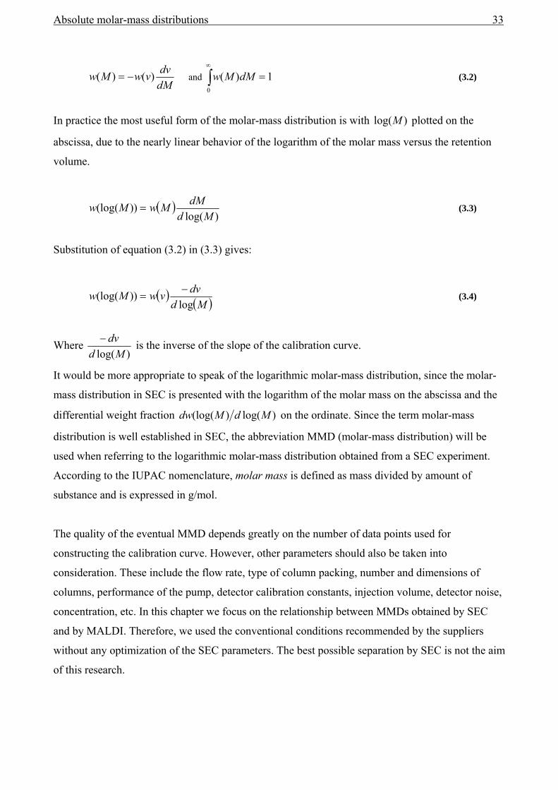
dMdvvwMw )()( −= and ∫
∞
=0
1)( dMMw (3.2)
In practice the most useful form of the molar-mass distribution is with )log(M plotted on the
abscissa, due to the nearly linear behavior of the logarithm of the molar mass versus the retention
volume.
( ))log(
))(log(Md
dMMwMw = (3.3)
Substitution of equation (3.2) in (3.3) gives:
( ) ( )MddvvwMw
log))(log( −= (3.4)
Where )log(Md
dv− is the inverse of the slope of the calibration curve.
It would be more appropriate to speak of the logarithmic molar-mass distribution, since the molar-
mass distribution in SEC is presented with the logarithm of the molar mass on the abscissa and the
differential weight fraction )log()(log( MdMdw on the ordinate. Since the term molar-mass
distribution is well established in SEC, the abbreviation MMD (molar-mass distribution) will be
used when referring to the logarithmic molar-mass distribution obtained from a SEC experiment.
According to the IUPAC nomenclature, molar mass is defined as mass divided by amount of
substance and is expressed in g/mol.
The quality of the eventual MMD depends greatly on the number of data points used for
constructing the calibration curve. However, other parameters should also be taken into
consideration. These include the flow rate, type of column packing, number and dimensions of
columns, performance of the pump, detector calibration constants, injection volume, detector noise,
concentration, etc. In this chapter we focus on the relationship between MMDs obtained by SEC
and by MALDI. Therefore, we used the conventional conditions recommended by the suppliers
without any optimization of the SEC parameters. The best possible separation by SEC is not the aim
of this research.

34 Chapter 3
3.2.1 Experimental
SEC analyses were preformed on a system that consisted of a three-column set (two PLgel Mixed-C
5 µm columns and one PLgel Mixed-D 5 µm column from Polymer Laboratories) with a guard
column (PLgel 5 µm, Polymer Laboratories), a gradient pump (Waters Alliance 2695, flow rate 1.0
mL/min isocratic), a photodiode-array detector (Waters 2996) and a differential refractive-index
detector (Waters 2414) as concentration detectors, a light-scattering detector (Viscotek), a viscosity
detector (Viscotek, dual detector 250). THF (Biosolve, Valkenswaard, the Netherlands) was used as
the solvent. THF was filtered twice (0.2 µm filter, Alltech, Breda, the Netherlands) and stabilized
with BHT (0.01 v%, Merck, >99% pure). Data acquisition was preformed with the Viscotek TriSec
GPC Software (version 3.0 Rev. B.03.04). All detectors were placed in series in the following
order: photodiode array (PDA), right-angle light scattering (RALS), viscosity (DP) and differential
refractive index (DRI).
3.3 Calibration methods in SEC
In SEC two types of standards are used, i.e. narrow standards with a narrow MMD and polymers
with a broad molar-mass distribution, but with known characteristic average values of the MMD.
Narrow standards were used for the calibration of the column, whereas some broad standards were
used to calibrate some instrument factors as discussed later.
The characteristic moments of the MMD are given by2:
( )
( )∫
∫∞
∞
⋅
⋅=
0
0
)(
)(
MdMMw
MdMwM n
( )
( )∫
∫∞
∞
⋅
⋅⋅=
0
0
)(
)(
MdMw
MdMMwM w
( )
( )∫
∫∞
∞
⋅⋅
⋅⋅=
0
0
2
)(
)(
MdMMw
MdMMwM z (3.5)
The polydispersity index (PDI) is expressed as:
n
w
MMPDI = (3.6)
Although some of these values are also reported for a calibration standard, it is the peak molar mass
( )pM which is used for constructing the calibration curve. The peak molar mass is located at the top
of the MMD measured by SEC and cannot be calculated from the moments of the MMD (Figure
3-1).

Absolute molar-mass distributions 35
Conventional calibration
By far the most frequently used method for calibration relies on the injection of narrow standards
(often polystyrenes). A large range of standards with different molar masses is chosen to cover the
entire mass range of the calibration curve. This method is known as conventional calibration. Note
that the ( )pM value is not sensitive to band-broadening effects.
The detectors used in this system to measure the concentration (DRI and PDA) do not require any
calibration, since relative concentrations suffice.
The quality of the model fitted to the calibration curve obviously influences the accuracy of the
MMD. Often a second- or third-order polynomial is used to describe the calibration curve and the
correlation coefficient ( )2R is used as indication of the quality of fit. The value of 2R is sensitive to
the selected order of the polynomial, especially since the number of injected standards is normally
rather limited (less then 20). A limited number of data points always provides an improvement of 2R with increasing order of the polynomial model and over-fitting is a danger. A statistically more-
justified parameter is the adjusted correlation coefficient 2adjR :
( )pn
nRRadj −−
⋅−−=111 22 (3.7)
Where R is the correlation coefficient, n is the number of data points, and p the number of
predictors or, in case of a polynomial fit, the order of the polynomial plus one. However, an
increase of the polynomial fit will still result in a value more close to unity. An alternative method
is suggested with the F-test comparison to test whether an alternative model gives a significant
improvement of the fit3. The F-test requires the standard deviations of the pM value and the
retention time as shown in Appendix 3E.
pM
nM wM
Retention volume
Intensity
Figure 3-1 The location of the different moments of an MMD and the location of pM .

36 Chapter 3
Universal calibration
As mentioned at the beginning of this chapter, the separation in SEC is based on the hydrodynamic
volumes of the molecules. The hydrodynamic volume ( )hV is defined as the product of the molar
mass and the intrinsic viscosity [ ]( )M⋅η . Plots of [ ]( )M⋅ηlog versus retention volume for all
polymers of different types, including different conformations (branched, grafted, cyclic, etc),
merge into a single plot. This curve, introduced by Benoit et al.4 is called the universal calibration
curve.
Each retention volume of an unknown sample in SEC corresponds to molecules of a given size and
thus a corresponding hydrodynamic volume. The unknown molar mass of a sample can be
calculated as long as the relation of hV vs. retention volume is known and the intrinsic viscosity
[ ]( )vη is measured. Since the relationship between hV and retention volume can be applied for all
polymers (the universal principle), the following relationship is obtained:
( ) [ ]( )h unknownV v v Mη= ⋅ (3.8)
Note, again that the quality of the calculated MMD depends on the accuracy of the model
describing ( )( )log hV v versus retention volume.
The empirical relation between molar mass and intrinsic viscosity is known as the Mark-Houwink
(MH) equation5:
[ ] K M αη = ⋅ (3.9)
Where α and K are constants for a given polymer, solvent and temperature, and M is the molar
mass. This relation can be used to express the intrinsic viscosities of Equation (3.8) in terms of
molar masses. However, the MH relationship is only valid for molar masses exceeding 20,000
g/mol6,7.
To measure the intrinsic viscosity Viscotek uses a four-capillary bridge-type cell, analogous to the
Wheatstone bridge (see Figure 3-2). The benefit of this instrument is the direct measurement of the
specific viscosity (ηsp).
DPIP
DPsp kDPkIP
kDP⋅⋅−⋅
⋅⋅=
24η (3.10)

Absolute molar-mass distributions 37
Where IP is the pressure difference across the bridge and DP is the differential pressure within the
bridge, DPk and IPk are the calibration factors of the pressure transducers. The setup of the
viscosity bridge was modified to put the detectors serial. The large-internal-diameter capillaries
used at the end of the bridge were replaced by narrow capillaries and the differential-refractive-
index detector was integrated in the bridge. Note, that this DRI detector was not used to determine
the concentrations of the polymer in the effluent, due to its low sensitivity. As mentioned in the
Experimental section, a Waters DRI detector was placed after the viscosity bridge. Since the old
DRI was integrated in the bridge, there was no time difference between the viscosity detector and
this detector. In this way the absolute time difference or volume difference could be determined
between the Waters DRI detector and the viscosity detector.
The viscosity constant visk is defined as DP
IP
kk . Substitution of visk into formula 3-10 gives:
DPkIPDP
vissp ⋅−⋅
⋅=
24η (3.11)
A viscosity detector yields the intrinsic viscosity [ ]( )η from the following equation:
[ ] ⎟⎟⎠
⎞⎜⎜⎝
⎛=
→ csp
c
ηη
0lim (3.12)
+ -
+
-
Flow in
Flow out
The viscosity bridge has four identical capillary resistors (8). The pressure difference is measured at two locations, across the bridge and inside the bridge. The pressure drop across the bridge is measured by the pressure transducers (1,6) whereas the pressure difference in the bridge is measured by pressure transducers (2,3). These four pressure transducers measure directly the specific viscosity. The sample cell of a DRI detector is placed inside the bridge (4) and the reference cell of the DRI detector is located at position 7. Under normal working conditions all valves (9) are closed. To purge the pressure transducers and the DRI reference cell, the valves are switched open. A hold-up reservoir of 19.94 mL is located at number 5. When the solution with the analyte enters the head of the bridge, the two capillary resistors (8a and 8b) will divide the flow ( ,Aφ Bφ ). Half way across the bridge 50% of the eluent will enter the large volume hold-up reservoir and the analyte gets diluted so effectively that the pressure difference between transducers 2 and 3 is totally dominated by the analyte passing capillary 8c. Note, the DRI detector is referred to as the old DRI detector in this section. It was not used for measuring concentrations. The analyte is diluted by approximately a factor of two due to the hold-up reservoir.
Figure 3-2 Scheme of the Viscotek viscosity detector
Aφ Bφ1
4
8b 8a
8d 8c
9
2 3
5
9 6
9
7

38 Chapter 3
0
0
ηηηη −
=sp (3.13)
where 0η is the viscosity of the solvent, η the viscosity of the sample solution, spη the specific
viscosity, c the concentration and rη the relative viscosity.
Two known methods to extrapolate the concentration to zero are given by Huggins8 and Kreamer9.
A practical alternative is the empirical Solomon-Gatesman equation which requires no extrapolation
and calculates [ ]η directly10,11. This method takes the averages of Huggins and Kraemer equations.
[ ] ( )c
spsp 1ln2 +−⋅=
ηηη (3.14)
Equation (3.11) and (3.14) can be used to determine visk by measuring standards of known intrinsic
viscosities and concentrations.
One of the major drawbacks of capillary viscometers is the presumed exact split of the flow at the
entrance of the bridge. When a polymer solution peak passes the cell, the pressure difference within
bridge may affect the presumed exact split of the flow. The shift of the peak due to a slight flow-
rate imbalance is known as the Lesec effect12,13. However, in our setup two DRI signals are
obtained, one from the old DRI detector in the bridge and the second one from the DRI detector
placed after the viscosity bridge, which is used to monitor the concentration. After the main peak
has emerged from the bridge and has been detected by the stand-alone (“new”) DRI, it takes some
19.94 mL before a second, shallow and broad peak, which represents the other half of the analyte,
can be observed.
Although the second peak was subject to serious band broadening, the areas of both the first and the
second chromatogram could still be used to measure the flow split.
The flow-fraction correction factor, frφ , was used to correct the concentrations, since the flow is not
exactly equally split at the entrance of the viscosity bridge.
BA
A
BA
Afr AreaArea
Area+
=+
=φφ
φφ (3.15)
Where Aφ and Bφ are the flows as shown in Figure 3-2 and AArea and BArea are the areas of the
main and the second peak, respectively.
At the end of the bridge, pure solvent from the delay column is mixed with the analyte which just
passed the right side of the bridge. As a result, the concentration will be a factor two lower than the

Absolute molar-mass distributions 39
concentration in the effluent. Moreover the DRI detector is placed after the viscosity bridge and it is
the only detector which measures the two-fold diluted sample. All other detectors experience the
“true” concentration. For calculations it is important to have the same concentrations for each
detector as explained in section 3.1.5. Note, that placing the DRI detector before the viscosity
bridge is not feasible at this moment, since DRI detectors can not withstand high back pressures.
No evidence could be found for the Lesec effect (increased flow imbalance with increasing molar
mass). With increasing molar mass and decreasing concentration the flow-rate fraction seemed to
approach unity and no bridge imbalance could be recorded.
Static light scattering
When the SEC system is equipped with a light scattering detector the absolute molecular-weight
distribution of a sample can be obtained. The expressions for wM , which can be found in many
textbooks are14:
( ) ( )2
32 321 cAcAPMR
cK
w
LS ++⋅
=∆
⋅θθ
(3.16)
Where, ( )θR∆ is the excess Rayleigh ratio (the difference between the Rayleigh ratio of the sample
solution and that of the pure solvent, where the Rayleigh ratio is defined as the scattered intensity at
the scattering angle θ ), c the concentration of the analyte, 2A and 3A are the second-, and third-
order virial coefficients, ( )θP is the dissymmetry factor, and LSK a constant defined as:
( )
ALS N
dcdnnK 40
220
24λ
π= (3.17)
Where 0n is the refractive index of the eluent, 0λ the wavelength in vacuum of the vertically
polarized incident light, AN the Avogadro number and ( )dcdn the specific refractive-index
increment, which accounts for the finite change in the eluent refractive index due to the presence of
analyte polymer.
In practice ( )θP is dependent on the angle between the laser and the detector cell and on the squared
radius of gyration or indirectly, the molar mass of the scattering molecules. In the setup, the angle
between the laser and the detector cell is fixed at 90 degrees. In the present system ( )θP equals
unity for molar masses below 200,000 g/mol. Molar mass exceeding 200,000 g/mol should be
interpreted with care. For the calculations of absolute wM values, methods are available to

40 Chapter 3
iteratively calculate the correct ( )θP for molar masses exceeding 200,000 g/mol, as can be found in
literature15. Methods to correct ( )θP will not be discussed since they are beyond the scope of this
work.
Equation (3.16) contains the unknown constants LSK , 2A and 3A . A recent study shows a negligible
influence of the third-order virial coefficient, which will therefore not be taken into account16. The
determination of the second-order virial coefficient requires a multi-angle-light-scattering
measurement, which was not preformed. Literature values were taken for the second order virial
coefficient ( =2A 286.00194.0 −⋅ wM ). However the concentrations in SEC are usually low and, hence,
the term cA2 (equation 2-13) is usually assumed negligible. The constant LSK requires knowledge
of the ( )dcdn values, as discussed in the next section.
Calibration of detector constants
In the previous sections the determination of the calibration constants for the viscosity and light-
scattering detectors were already discussed. However, the local concentrations are needed for the
calculations of the intrinsic viscosity and the MMD from light scattering.
The concentration detectors, photodiode array (PDA) and differential refractive index (DRI), were
used to calculate the actual concentrations. A PDA detector covers a range of wavelengths. The
absorbance at each particular wavelength follows the Lambert-Beer law.
cb ⋅⋅= εAbsorbance (3.18)
Where ε is the molar absorption coefficient, b the path length of the cell, and c the analyte
concentration.
The following relations were used:
PDA
PDA kvyvc)(
),(),(λλλ = (3.19)
( )( ) injsample
PDA
injsample
PDAPDA Vcd
dvvcdVc
dvvck 1),(),(
)( ⋅=⋅
= ∫∫ λλλ (3.20)
( )( ) 2
( ) frDRI
DRI
y vc v
k dn dcφ⋅
=⋅
(3.21)
( )
( )( )( )
( ) ( )2 2fr fr
DRIsample inj injsample
d y v dvy v dvk
c V dn dc V dn dcd c
φ φ⋅ ⎛ ⎞= = ⋅⎜ ⎟⎜ ⎟⋅ ⋅ ⋅⎝ ⎠
∫∫ (3.22)

Absolute molar-mass distributions 41
Where ( )vy is the response of the DRI detector at an elution volume v , ( )λ,vy is the response of
the PDA detector at an elution volume v and a given wavelength (λ ) , samplec the known
concentration of a sample, ( )DRIc v the local concentration of the sample, ( )dcdn the specific
refractive index increment, injV the injection volume, ( )( )
( )samplecd
dvvyd ∫ the slope obtained from the area
of the raw SEC data chromatograms versus the known injected concentrations, frφ the flow-rate
fraction of the viscosity bridge (see paragraph 2.1.3), DRIk the DRI calibration factor, and PDAk the
PDA calibration factor.
To correct for the sample dilution after the viscosity bridge, frφ has to be multiplied by a factor of
two.
The value of DRIk is still dependent on the value of ( )dcdn , whereas PDAk is dependent on the
value of ε . Unfortunately, both the values of ( )dcdn and of ε are dependent of the molar mass
and/or the end groups. The ( )dcdn of polystyrene in THF becomes constant when the molar mass
exceeds 10,000 g/mol17. The empirical relationship between molar mass and ( )dcdn can be
written as:
( ) bdn dc aM
= + (3.23)
Where a and b are constants and M is the molar mass. The ( )dn dc value is mainly affected for
molar masses under 1000 g/mol.
The last system-dependent correction is the inter-detector-delay volume. The consequence of
connecting detectors in series is a time lag between the detectors. Moreover, the calculation of the
intrinsic viscosity requires knowledge of the concentration and the specific viscosity of the same
sample volume, which is detected at different times. The determination of the time lag between the
viscosity and DRI detectors was already discussed in section 2.1.3. The time lag between a UV
detector and a DRI detector can be simply determined by the volume difference, the so-called the
inter-detector-delay volume, between the corresponding observed maxima in the detector responses.
However, the inter-detector-delay of the light-scattering-detector and the DRI detector cannot be
determined by the observed maxima in the detector responses. The light-scatting-detector response
is proportional to the product of the concentration and the molar mass (formula 2-13), whereas the
response of the DRI detector is only proportional to the concentration. No attempt was made to

42 Chapter 3
correct for the difference in responses. Instead of using a narrowly distributed standard, a broad
standard with known molar-mass averages was used to determine the inter-detector-delay volume.
Note, that the other constants of the light-scattering detector can be determined independently of the
inter-detector-delay volume, since they only require the total peak areas.
3.4 Band broadening in SEC
A known phenomenon in SEC is band broadening, which obviously affects the experimentally
determined MMD. In this work all band-broadening effects are merged into one parameter ( )σ .
Different types of band broadening are extensively discussed elsewhere18.
A concentration profile of a sample in a column is subjected to band broadening when it passes
through a column. The relation between the MMD and the Gaussian band broadening is given by
Tung’s19 equation:
( ) ( ) ( )1 1 1y v w v G v v dv= ⋅ −∫ (3.24)
Where ( )1vw is the unbiased true MMD, ( )y v the experimental SEC chromatogram, v and 1v are
the respective retention volumes, and ( )vG is the Gaussian band-broadening function. The MMD
can be corrected directly, so that equation (3.24) can be written in a more useful form20:
( )( )
( )( ) MdMw
dvMd
MM
dvMd
Mw loglog2log
log'logexp2log
1)'(log0 2
2
2
⋅⋅
⎟⎟⎟⎟⎟
⎠
⎞
⎜⎜⎜⎜⎜
⎝
⎛
⋅⎟⎠⎞
⎜⎝⎛
−
−−
⋅⋅⎟⎠⎞
⎜⎝⎛
−⋅
= ∫∞
σπσ (3.25)
where σ is the dispersion constant, ( )⎟⎠⎞
⎜⎝⎛
− dvMd log the slope of the calibration curve, )'(log Mw the
apparent MMD and )(log Mw the “true” MMD . Many researchers19,21-25 put a lot of effort in
solving Equation (3.25) for )(log Mw . Strictly speaking, the exact solution of Equation (3.25)
requires the “true” MMD to be known and is therefore very hard to obtain.
An alternative method to estimate the effect of band broadening in SEC involves using a longer
column. That would allow an assessment of the effect of the importance of band broadening in the
SEC in comparison with MALDI. In order to be able to compare the experimentally determined
MMDs from SEC and from MALDI, the latter was subjected to an artificial band-broadening effect.
The details of this procedure will be discussed in Chapter 4.

Absolute molar-mass distributions 43
3.5 Results
Some calibration curves require the calibration constants to be known. Therefore the calibration
constants will be discussed first.
The calibration constants are either system dependent or eluent dependent. Note that none of the
calibration parameters in Table 1 are affected by the column performance.
Table 1 Calibration parameters for the calculation of the molar-mass distribution (MMD).
System-dependent parameters Eluent-dependent parameters
04.0065.1 ±=visk ( ) 002.0185.0 ±=dcdn mg/g
010.0530.0 ±=−LSDRIIDD mL 55 1002.01018.1 −− ⋅±⋅=LSK
010.0422.0 ±=−DPDRIIDD mL 4611699±=DRIk mV
0.0040.660±=−UVDRIIDD mL 378602±=PDAk mV
0.988 0.012frφ = ±
The pressure difference measured by the pressure transducers is recorded in Volts. The value of visk
close to unity implies that the conversion from Volts to Pascals is nearly the same for both
transducers.
The inter-detector-delays (IDDs) were calculated from the time difference between the pM values
for all standards. An average value was calculated (see appendix 3A). The correct LSDRIIDD − could
not be obtained from the pM values as explained in section 3.1.5. Broad standards of known
average molar-masses were used to fit the LSDRIIDD − . Since only a limited number of broad
standards were measured, the standard deviation of the LSDRIIDD − was computed from the
pM values.
The calculated frφ is close to unity, which implies that the splitting performs very well. A value
lower than one means that slightly less than half of the solution takes the short path through the
viscosity bridge and that the concentration measured by the DRI represents slightly less than half of
the total analyte.
The ( )dcdn value and its standard deviation were taken from literature14.
No significant influence was observed of the second virial coefficient in determining LSK , due to
the low (enough) concentrations. The standards with molar masses exceeding 200,000 g/mol were
neglected due to the angle dependence (section 0). The DRIk and PDAk values were calculated as
described in section 0.
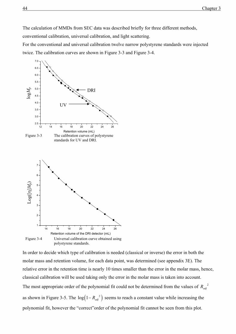
44 Chapter 3
The calculation of MMDs from SEC data was described briefly for three different methods,
conventional calibration, universal calibration, and light scattering.
For the conventional and universal calibration twelve narrow polystyrene standards were injected
twice. The calibration curves are shown in Figure 3-3 and Figure 3-4.
In order to decide which type of calibration is needed (classical or inverse) the error in both the
molar mass and retention volume, for each data point, was determined (see appendix 3E). The
relative error in the retention time is nearly 10 times smaller than the error in the molar mass, hence,
classical calibration will be used taking only the error in the molar mass is taken into account.
The most appropriate order of the polynomial fit could not be determined from the values of 2adjR
as shown in Figure 3-5. The ( )2log 1 adjR− seems to reach a constant value while increasing the
polynomial fit, however the “correct”order of the polynomial fit cannot be seen from this plot.
Figure 3-4 Universal calibration curve obtained using polystyrene standards.
14 16 18 20 22 24 261
2
3
4
5
6
7
Retention volume of the DRI detector (mL)
Log(
[η]M
p)
Figure 3-3 The calibration curves of polystyrene standards for UV and DRI.
logM
p
12 14 16 18 20 22 24 262.5
3.0
3.5
4.0
4.5
5.0
5.5
6.0
6.5
7.0
Retention volume (mL)
UV
DRI

Absolute molar-mass distributions 45
To perform a F-test the standard deviation of the molar mass need to be known. The molar mass
values provided by MALDI and SEC were used to calculate the molar mass error of each data
point. The F-test comparison method was used to validate whether an increase of the polynomial
order is significant as described elsewhere3. For all calibration curves a fifth- or sixth-order
polynomial was used (see appendix 3F).
For the sake of completeness the Mark-Houwink (MH) constants were determined.
A plot of the logarithm of the intrinsic viscosity versus the logarithm of the molar mass can be used
to obtain the MH constants, as shown in Figure 3-6. A clear deviation from the linear MH
relationship was observed for molar masses below 20,000 g/mol. A third-order polynomial was
used to cover the entire mass range (1050– 3.8 610 g/mol). If the principle of universal calibration
can be applied and the molar masses are below 20,000 g/mol, then the third-order polynomial is
recommended.
1 2 3 4 5 6 7
1E-5
1E-4
1E-3
Universal calibration Conventional calibration UV Conventional calibration DRI
Figure 3-5 ( )2log 1 adjR− versus the order of the polynomial equation used to fit the
calibration curves of Figure 3-3 and Figure 3-4.
Polynomial fit order
(1-Radj 2)
2.5 3.0 3.5 4.0 4.5 5.0 5.5 6.0 6.5 7.0
-1.5
-1.0
-0.5
0.0
0.5
1.0
logM
Figure 3-6 Relationship between intrinsic viscosity and molar mass. All polystyrene standards were injected twice. The dashed line represents the linear MH equation. The solid line represents a third-order polynomial.
Log[η]
[ ] 013.0707.0000004.0000138.0 ±⋅±= Mη

46 Chapter 3
After all calibration parameters were determined, four broad standards were measured. The fourth
standard is a blend of narrow polystyrene standards as will be discussed in Chapter 4. Some of the
characteristic values from literature are given in Table 2.
All calculated characteristic values of the four standards are given in Appendix 3A with the
calibration-parameter values listed in Table 1.
An alternative method to calculate nM , the Goldwasser26 method, is extremely sensitive for
baseline settings and is, unfortunately, of no practical use. No attempts were made to optimize the
nM values obtained by the Goldwasser method, since the necessary slight changes in baseline
settings had no significant effect on the characteristic values as obtained from the other methods.
Table 2 The characteristic values of broad standards of polystyrene as listed in literature.
nM g/mol wM g/mol [ ]η dl/g e
Dow 1683a 100,000 250,000 0.843
Dow 1683b 95,930 242,900 -
PS 280 c - 274,126 0.891
SRM 706 d - 285,000 +/- 2000 -
a) American Polymer Standards Corporation, b) International GPC symposium 1996, J.Lesec and M.Millequant, pg. 87, c) Viscotek Cooperation, d)
National Institute of Standards and Technology (NIST) .
e) Eluent THF at 30 °C
Table 3 shows the obtained moments for two different parameter settings. It is at least remarkable,
that the values of the PS280 ( wM , [ ]η ) seem to agree very well with the values given in Table 2
whereas the other values of the broad standards deviate from the corresponding literature values.
The wM of Dow 1683 and the SRM 706 are both too far off (see Table 3, method 1).
Table 3 Deviations of the broad standards for both parameters settings using light scattering as calibration method.
Method 1† Method 2*
nM g/mol wM g/mol nM g/mol wM g/mol
Dow 1683 97,550 266,600 101,400 255,400
PS 280 123,400 276,650 125,550 265,100
SRM 706 123,900 296,400 126,750 284,500
Deviation Dow 1683 (%) -0.4 8.2 0.4 3.0
Deviation PS 280 (%) - 0.9 - -4.2
Deviation SRM 706 (%) - 4.0 - -1.3
† The parameter settings for each method are listed in Appendix 3A-3B.

Absolute molar-mass distributions 47
A much better agreement between the standards of Dow 1683 and SRM 706 (see Table 3, method
2) is found in appendix 3B, where only a few calibration parameters were adjusted.
For further calculations the second calibration-parameter settings were chosen. A very thorough
study has recently been published on obtaining the accurate wM of the SRM 70616.
Error analysis
Erroneous MMDs are the result of propagating errors of calibration methods, calibration constants,
variation in system performance and erroneous reference data.
Reference materials
The pM values of standards materials are given by the supplier, but rarely the standard deviation is
reported. Since there is no absolute method to directly measure the pM value of a narrow standard,
one should rely on the nM and wM determined by classical methods or by mass spectrometry i.e.
MALDI.
The pM values obtained by MALDI were found to be in excellent agreement with the pM values
given by the supplier (appendix 3E). The transformation of the MALDI distribution to a w(logM)
distribution, as in SEC, is described in more detail in Chapter 4. However, the transformation hardly
affects the value of pM (except for molar masses below 2,000 amu). In order to obtain the pM
value from a MALDI spectrum, the entire distribution is converted to a w(logM) distribution. The
conversion is discussed in detail in Chapter 4.
Moreover, the universal calibration curve requires, besides the same pM values, the known
intrinsic viscosities of the polymer standards, making this calibration method more error-sensitive
than conventional calibration.
Calibration method
Different methods for calibration have been tested to obtain the MMD. Instead of looking at the
entire MMD, the average molar masses ( nM , wM and zM ) are compared for each calibration
method. Unfortunately the unbiased absolute moments for the broad distributions are unknown as
references. It is assumed that light scattering provides the most reliable moments and, therefore, all
moments are compared to the average molar masses obtained by light scattering. The values are
shown in Table 4.

48 Chapter 3
Table 4 The relative deviation obtained for conventional calibration (CC) and universal calibration (UC). All
calibration methods are compared to the moments obtained by light scattering of the standard SRM 706.
moments CC-LS deviation (%) UC-LS deviation (%)
nM g/mol 0.8 -3.8
wM g/mol -0.8 -1.7
zM g/mol -5.7 -6.1
Calibration-parameter uncertainties affecting the moments calculated by light scattering
To investigate the effect of all calibration-parameter uncertainties, again the average molar masses
are computed and their deviation reported. The values of the root-mean-squares (RMS) are listed in
Table 5 expressed in g/mol for the broad standard PS280. The relative contributions of the
uncertainties of all calibration parameters can be found in appendix 3C. The values for wM , zM
were strongly affected by the uncertainty of the LSK . The value of nM was strongly affected by
the uncertainty of LSDRIIDD − .
Table 5 The errors in the calculated characteristic values of the
polystyrene PS280 broad standard.
Target value RSM (g/mol) Std. dev. %
nM g/mol 123,100 4,788 4.1
wM g/mol 276,500 5,244 2.2
zM g/mol 423,300 5,993 1.8
System performance
Since there are always small variations in the SEC performance the maximum error among all
reinjected broad standards is reported in Table 6.
Table 6 The maximum relative error among all reinjected broad standards.
Max. error %
nM g/mol 2.7
wM g/mol 2.0
zM g/mol 4.2
An overview of the various sources of error is given in table 7.

Absolute molar-mass distributions 49
Table 7 Overview of the maximum error in the molar-mass moments.
Calibration curve Light scattering Repeatability
Max. error % Std. dev. % Max. error % Tot. Max error. %
nM g/mol 3.8 4.1 2.7 <5%
wM g/mol 1.7 2.2 2.0 <2.5 %
zM g/mol 6.1 1.8 4.2 <7.5%
The presented errors do not represent an in-depth thorough study or a full error analysis and should
be interpreted with some care. In this example, the average molar masses of the MMD were used to
indicate the quality of the calibration parameters. However, the best calibration for light scattering
and viscosity measurements requires a complete analysis of a sample including, the molar mass, the
intrinsic viscosity, the radius of gyration, the hydrodynamic radius, all moments of these molar-
mass distribution, and the MH constants. Each calibration parameter affects at least one of these
values in different ways. If each calibration parameter responds in different ways, then errors may
cancel or amplify each other. Such a thorough error analysis is beyond the scope of this thesis.
Axial dispersion corrections
Practical experience shows that axial-dispersion corrections have a limited effect on the computed
average molar-masses of the MMD, but strongly affect e.g. the values of the MH constants. Due to
their limited effect on the MMD no further attempts were made to optimize the axial-dispersion
correction parameters.
3.6 Conclusions
Calibration methods were compared for one purpose only, i.e. to obtain the most accurate MMD.
Besides conventional calibration, there are many parameters that affect the outcome of the MMD in
more-advanced calibration methods, such as universal calibration and triple detection (no need for a
calibration curve). A pragmatic approach to determine each parameter carefully (and
independently) did not yield the best results. The calibration parameters, such as light-scattering
constant LSK and LSDRIIDD − required adjustment to obtain significantly better results. These two
parameters turned out to be the most critical parameters in the determination of the MMD moments.
Throughout all the measurements, conventional calibration and light-scattering detection seemed to
correspond rather well, whereas somewhat larger differences were found for universal calibration.
In the end, if the molar masses are not too high (<500,000 g/mol) and the absolute MMD is required
within less than one percent error, fractionation of the sample and MS analysis seems to be a (very)

50 Chapter 3
attractive alternative, at least within the limits of applicability of MALDI-TOF-MS.

Absolute molar-mass distributions 51
Reference List 1. Mori, S.; Barth, H. G. Size Exclusion Chromatography, Springer-Verlag, Berlin Heidelberg
New York, 1999.
2. Shortt, D. W. Journal of Liquid Chromatography 1993, 16 (16), 3371-3391.
3. van Herk, A. M. Journal of Chemical Education 1995, 72, 138-140.
4. Grubisic, Z.; Rempp, P.; Benoit, H. J Polym Sci Polym Lett Ed 1967, 5, 753.
5. Sakurada, I. Kolloid Z. 1938, 82, 345.
6. Fox, T. G.; Kinsinger, J. B.; Mason, H. F.; Schuele, E. M. Polymer 1962, 3, 71.
7. Altares, T.; Wyman, D. P.; Allen, V. R. J Polym Sci Polym Lett Ed 1964, A2, 4533.
8. Huggins, M. L. J. Am. Chem. Soc. 1942, 64, 2716.
9. Kraemer, E. O. Ind. Eng. Chem. 1938, 30, 1200.
10. Solomon, O. F.; Gotesman, B. S. Makromol. Chem. 1967, 104, 177.
11. Solomon, O. F.; Ciuta, I. Z. J. Appl. Polym. Sci. 1962, 6, 683.
12. . Abstr. Pap. Am. Chem. Soc. 1993, 206 (130-PMSE).
13. Lesec, J.; Millequant, M.; Havard, T. ACS Symp. Ser. 1993, 521, 220-230.
14. Mori, S.; Barth, H. G. Size Exclusion Chromatography, Springer-Verlag, Berlin Heidelberg New York, 1999.
15. Mori, S.; Barth, H. G. Size Exclusion Chromatography, Springer Verlag Berlin Heidelberg New York, 1999.
16. Guttman, C. M.; Blair, W. R.; Fanconi, B. M.; Goldschmidt, R. J.; Wallace, W. E.; Wetzel, S. J.; VanderHart, D. L. NIST Special Publication 2003, 260-152.
17. Bahr, U.; Deppe, A.; Karas, M.; Hillenkamp, F.; Anal. Chem. 1992, 64, 2866-2869.
18. Popovici, S. Towards Smal and Fast Size-Exclusion Chromatography, PhD Thesis, University of Amsterdam 2004.
19. Tung, L. H. J. Appl. Polym. Sci. 1966, 10, 375.
20. Tung, L. H.; Runyon, J. R. J. Appl. Polym. Sci. 1969, 13, 2397-2409.
21. Meira, G. R. "Data reduction in size exclusion chromatography" in Modern Methods of Polymer Characterization, H. G. Barth, J. W. Mays, eds (Wiley, New York) 1991.
22. Styring, M. G.; Hamielec, A. E. "Determination of Molecular Weight Distribution by Gel Permeation Chromatography", Determination of Molecular Weight, A. R. Cooper, ed., Wiley, New York 1989.
23. Hamielec, A. E. "Correction for Axial Dispersion", Steric Exclusion in Liquid Chromatography of Polymers, J. Janka, ed., Dekker, New York 1984.

52 Chapter 3
24. Yau, W. W.; Kirkland, J. J.; Bly, D. D. Modern Size-Exclusion Liquid Chromatography, Wiley, New York 1979.
25. Yau, W. W.; Stoklosa, H. J.; Bly, D. D. J. Appl. Polym. Sci. 1977, 21 (1911).
26. Goldwasser, J. M. International GPC Symposium, Newton, MA, October 1989.
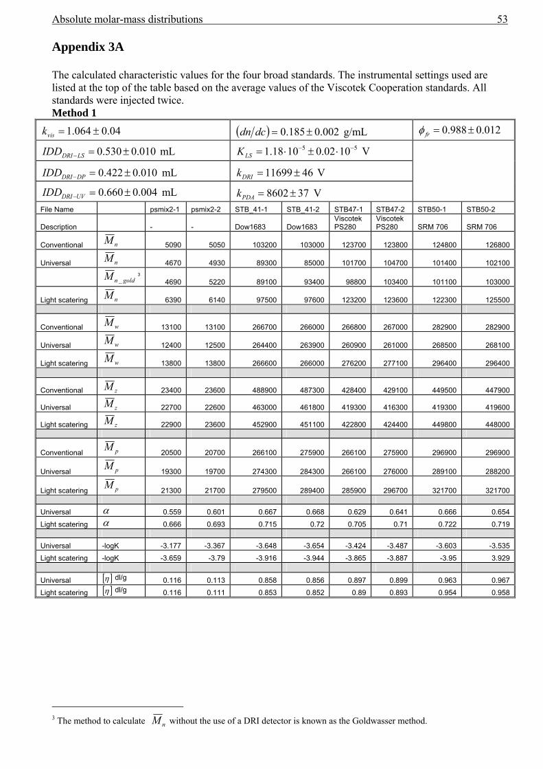
Absolute molar-mass distributions 53
Appendix 3A The calculated characteristic values for the four broad standards. The instrumental settings used are listed at the top of the table based on the average values of the Viscotek Cooperation standards. All standards were injected twice. Method 1
04.0064.1 ±=visk ( ) 002.0185.0 ±=dcdn g/mL 0.988 0.012frφ = ±
010.0530.0 ±=−LSDRIIDD mL 55 1002.01018.1 −− ⋅±⋅=LSK V
010.0422.0 ±=−DPDRIIDD mL 4611699±=DRIk V
0.0040.660±=−UVDRIIDD mL 378602±=PDAk V
File Name psmix2-1 psmix2-2 STB_41-1 STB_41-2 STB47-1 STB47-2 STB50-1 STB50-2
Description - - Dow1683 Dow1683 Viscotek PS280
Viscotek PS280 SRM 706 SRM 706
Conventional nM 5090 5050 103200 103000 123700 123800 124800 126800
Universal nM 4670 4930 89300 85000 101700 104700 101400 102100
goldnM _3 4690 5220 89100 93400 98800 103400 101100 103000
Light scatering nM 6390 6140 97500 97600 123200 123600 122300 125500
Conventional wM 13100 13100 266700 266000 266800 267000 282900 282900
Universal wM 12400 12500 264400 263900 260900 261000 268500 268100
Light scatering wM 13800 13800 266600 266000 276200 277100 296400 296400
Conventional zM 23400 23600 488900 487300 428400 429100 449500 447900
Universal zM 22700 22600 463000 461800 419300 416300 419300 419600
Light scatering zM 22900 23600 452900 451100 422800 424400 449800 448000
Conventional pM 20500 20700 266100 275900 266100 275900 296900 296900
Universal pM 19300 19700 274300 284300 266100 276000 289100 288200
Light scatering pM 21300 21700 279500 289400 285900 296700 321700 321700
Universal α 0.559 0.601 0.667 0.668 0.629 0.641 0.666 0.654
Light scatering α 0.666 0.693 0.715 0.72 0.705 0.71 0.722 0.719
Universal -logK -3.177 -3.367 -3.648 -3.654 -3.424 -3.487 -3.603 -3.535
Light scatering -logK -3.659 -3.79 -3.916 -3.944 -3.865 -3.887 -3.95 3.929
Universal [ ]η dl/g 0.116 0.113 0.858 0.856 0.897 0.899 0.963 0.967
Light scatering [ ]η dl/g 0.116 0.111 0.853 0.852 0.89 0.893 0.954 0.958
3 The method to calculate nM without the use of a DRI detector is known as the Goldwasser method.

54 Absolute molar-mass distributions
Appendix 3B The calculated characteristic values for the four broad standards. The instrumental settings used are listed at the top of the table and based on the average values of the DOW 1683 and the SRM 706. All standards were injected twice. Method 2
04.0050.1 ±=visk ( ) 002.0185.0 ±=dcdn mL/g 0.988 0.012frφ = ±
010.0510.0 ±=−LSDRIIDD mL 55 1002.01012.1 −− ⋅±⋅=LSK V
010.0410.0 ±=−DPDRIIDD mL 4611699±=DRIk V
0.0040.660±=−UVDRIIDD mL 378602±=PDAk V
File Name psmix2-1 psmix2-2 STB_41-1 STB_41-2 STB47-1 STB47-2 STB50-1 STB50-2
Description - - Dow1683 Dow1683 Viscotek PS280
Viscotek PS280 SRM 706 SRM 706
Conventional nM 5090 5060 103300 103200 124000 124000 125000 126600
Universal nM 4920 5200 107400 104500 115100 118300 120600 117800
goldnM _4 5900 5500 83200 95400 100600 105100 103000 103200
Light scatering nM 5440 4890 101400 101400 124600 126500 125600 127900
Conventional wM 13200 13100 266100 265500 266200 266400 282300 282200
Universal wM 12800 12900 278400 276400 271300 271400 280200 279000
Light scatering wM 13400 13600 255600 255200 264300 265900 284600 284400
Conventional zM 23600 23400 485100 483700 425300 425300 446200 444600
Universal zM 23200 22900 516300 506200 446400 443000 448900 445500
Light scatering zM 24000 25500 420300 419400 394900 397000 422200 420400
Conventional pM 20500 20700 266100 275900 266100 275900 296900 296900
Universal pM 20000 20400 276600 288000 270600 280800 294600 294200
Light scatering pM 20800 21500 270800 280000 276400 286700 310700 310500
Universal α 0.565 0.608 0.671 0.672 0.632 0.644 0.666 0.654
Light scatering α 0.608 0.636 0.728 0.734 0.707 0.717 0.725 0.721
Universal -logK -3.216 -3.409 -3.685 -3.689 -3.455 -3.519 -3.622 -3.553
Light scatering -logK -3.408 -3.534 -3.984 -4.014 -3.867 -3.918 -3.956 -3.936
Universal [ ]η dl/g 0.114 0.112 0.844 0.843 0.882 0.884 0.945 0.948
Light scatering [ ]η dl/g 0.114 0.112 0.844 0.843 0.882 0.885 0.945 0.948
4 The method to calculate nM without the use of a DRI detector is known as the Goldwasser method.
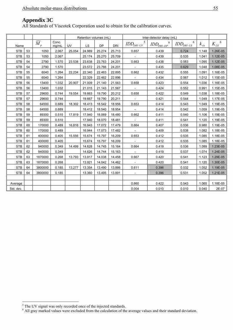
Absolute molar-mass distributions 55
Appendix 3C All Standards of Viscotek Corporation used to obtain for the calibration curves. Retention volumes (mL) Inter-detector delay (mL)
Name pM Conc. mg/mL UV LS DP DRI UVDRIIDD −
5 DPDRIIDD −
6 LSDRIIDD −
6 visk LSK 6
STB 53 1050 2.067 25.054 24.989 25.274 25.713 0.657 0.439 0.724 1.148 1.26E-05
STB 53 1050 2.067 25.174 25.270 25.709 - 0.439 0.535 1.041 1.12E-05
STB 54 2790 1.570 23.538 23.638 23.763 24.201 0.663 0.438 0.563 1.095 1.12E-05
STB 54 2790 1.570 23.572 23.766 24.201 - 0.435 0.629 1.048 1.08E-05
STB 55 6040 1.264 22.234 22.340 22.463 22.895 0.662 0.432 0.555 1.091 1.16E-05
STB 55 6040 1.264 22.329 22.462 22.896 - 0.434 0.567 1.012 1.15E-05
STB 56 13400 1.032 20.907 21.009 21.140 21.563 0.658 0.423 0.554 1.036 1.16E-05
STB 56 13400 1.032 21.015 21.143 21.567 - 0.424 0.552 0.991 1.15E-05
STB 57 29600 0.744 19.554 19.663 19.790 20.212 0.658 0.422 0.549 1.038 1.18E-05
STB 57 29600 0.744 19.667 19.790 20.211 - 0.421 0.544 1.049 1.17E-05
STB 58 64500 0.689 18.302 18.413 18.542 18.956 0.653 0.414 0.543 1.049 1.19E-05
STB 58 64500 0.689 18.412 18.540 18.954 - 0.414 0.542 1.059 1.19E-05
STB 59 89300 0.510 17.819 17.940 18.069 18.480 0.662 0.411 0.540 1.106 1.19E-05
STB 59 89300 0.510 17.940 18.070 18.481 - 0.411 0.541 1.120 1.19E-05
STB 60 170000 0.489 16.816 16.943 17.072 17.479 0.664 0.407 0.536 0.980 1.19E-05
STB 60 170000 0.489 16.944 17.073 17.482 - 0.409 0.538 1.082 1.18E-05
STB 61 400000 0.405 15.556 15.674 15.797 16.209 0.653 0.412 0.535 1.085 1.18E-05
STB 61 400000 0.405 15.674 15.797 16.209 - 0.412 0.535 1.085 1.18E-05
STB 62 940000 0.349 14.499 14.628 14.745 15.164 0.664 0.419 0.536 1.089 1.23E-05
STB 62 940000 0.349 14.626 14.744 15.163 - 0.419 0.537 1.074 1.24E-05
STB 63 1870000 0.268 13.793 13.917 14.038 14.458 0.667 0.420 0.541 1.123 1.29E-05
STB 63 1870000 0.268 13.921 14.042 14.462 - 0.420 0.541 1.120 1.30E-05
STB 64 3800000 0.185 13.277 13.354 13.490 13.886 0.611 0.396 0.532 1.052 1.19E-05
STB 64 3800000 0.185 13.360 13.495 13.891 - 0.396 0.531 1.052 1.21E-05
Average 0.660 0.422 0.543 1.065 1.18E-05
Std. dev. 0.004 0.010 0.010 0.040 2E-07
5 The UV signal was only recorded once of the injected standards. 6 All gray marked values were excluded from the calculation of the average values and their standard deviation.
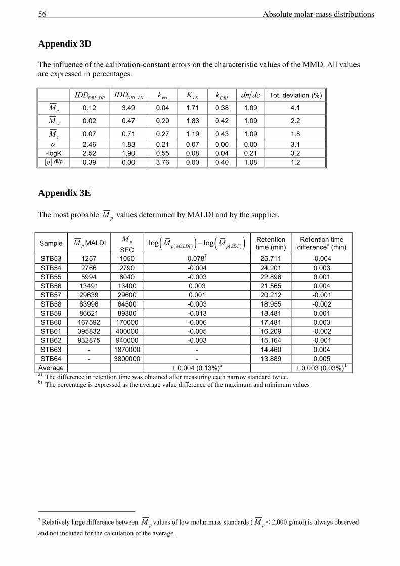
56 Absolute molar-mass distributions
Appendix 3D The influence of the calibration-constant errors on the characteristic values of the MMD. All values are expressed in percentages.
DPDRIIDD − LSDRIIDD − visk LSK DRIk dcdn Tot. deviation (%)
nM 0.12 3.49 0.04 1.71 0.38 1.09 4.1
wM 0.02 0.47 0.20 1.83 0.42 1.09 2.2
zM 0.07 0.71 0.27 1.19 0.43 1.09 1.8 α 2.46 1.83 0.21 0.07 0.00 0.00 3.1
-logK 2.52 1.90 0.55 0.08 0.04 0.21 3.2 [ ]η dl/g 0.39 0.00 3.76 0.00 0.40 1.08 1.2
Appendix 3E The most probable pM values determined by MALDI and by the supplier.
a) The difference in retention time was obtained after measuring each narrow standard twice. b) The percentage is expressed as the average value difference of the maximum and minimum values
7 Relatively large difference between pM values of low molar mass standards ( pM < 2,000 g/mol) is always observed and not included for the calculation of the average.
Sample pM MALDI pM SEC
( )( ) ( )( )log logp MALDI p SECM M− Retention time (min)
Retention time differencea (min)
STB53 1257 1050 0.0787 25.711 -0.004 STB54 2766 2790 -0.004 24.201 0.003 STB55 5994 6040 -0.003 22.896 0.001 STB56 13491 13400 0.003 21.565 0.004 STB57 29639 29600 0.001 20.212 -0.001 STB58 63996 64500 -0.003 18.955 -0.002 STB59 86621 89300 -0.013 18.481 0.001 STB60 167592 170000 -0.006 17.481 0.003 STB61 395832 400000 -0.005 16.209 -0.002 STB62 932875 940000 -0.003 15.164 -0.001 STB63 - 1870000 - 14.460 0.004 STB64 - 3800000 - 13.889 0.005
Average ± 0.004 (0.13%)b ± 0.003 (0.03%) b

MALDI-SEC 57
Appendix 3F To check whether an alternative model B gives a significant improvement of the fit over model A, the following statistical test was made:
( ) ( )
( ) ( ),
A
BA B
z A B A
A
A
ssss
p p F p p i pss
i p
ΘΘ −
−≥ − −
Θ
−
(A3-1)
Where ( ),z A B AF p p i p− − represents a value from the F-distribution at level z and at ,A Bp p and Ai p− degrees
of freedom and ( ) ( ),A Bss ssΘ Θ the estimated sum of squares. The model B represents a higher polynomial fit order
then model A.
Polynomial order ( ) ( )
( )
A
BA B
A
A
ssss
p pss
i p
ΘΘ −
−
Θ
−
( ),z A B AF p p i p− −
DRI UV Universal DRI UV Universal 2 20.4 45.3 188.8 4.5 4.3 4.4 3 52.4 70.1 26.9 4.6 4.4 4.4 4 16.1 25.6 8.5 4.7 4.4 4.5 5 5.9 63.1 7.6 4.7 4.4 4.5 6 0.2 27.6 2.2 4.8 4.5 4.5 7 0.2 3.7 0.4 5.0 4.5 4.6
Appropriate polynomial order 5 6 5
The appropriate polynomial order is based on the criterion given by equation A3-1.

58 Chapter 4

MALDI-SEC 59
Chapter 4
4 The relationship between the MMD from MALDI and from SEC
4.1 Introduction
In case of a homopolymer, the main limiting factor that stands between MALDI and the MMD is
formed by ionization-efficiency differences within samples that are heterogeneous in terms of size,
mass or chain length. This phenomenon, which is generally denoted as mass discrimination makes
the determination of molar-mass distributions (MMD) by MALDI an ongoing challenge.
Various publications1-8 have shown that accurate MMDs can be obtained for polymers with a
narrow MMD or low polydispersity index (PDI<1.2). However, for samples with a high
polydispersity, both underestimation and overestimation of the high-mass fractions have been
reported9,10. In the literature many factors have been reported to contribute to mass discrimination.
These include sample preparation, desorption/ionization mechanisms, ion focusing/transmission,
mass-dependent detection and detector saturation. All these factors contribute to an erroneous
MMD.
Concerning mass discrimination, it is our experience that the recently reported matrix, trans-2-[3-
(4-tert-butylphenyl)-2-methyl-2-propenylidene]malononitrile (DCTB)11, exhibits significantly less
mass than other commonly used matrices. Mass discrimination can be investigated by the
comparison of molar-mass distributions obtained by methods without mass discrimination such as
SEC. Besides the fact that SEC is a relative method, SEC and MALDI-TOF-MS data are presented
in a different way, as logarithmic molar-mass distributions and number distributions, respectively.
In order to compare the two distributions, the conversion of MALDI-TOF-MS spectra to a
logarithmic molar-mass distribution requires careful attention. Numerous authors compare average

60 Chapter 4
values of the MMD (number molar-mass and weight-average molar mass), whereas only very few
authors12,13 compare the total MMD. Moreover, the suggested methods for comparing these
distributions are not always consistent.
In this chapter mass discrimination will be quantitatively investigated by comparing MMDs
obtained by different methods of calibration in Size-Exclusion Chromatography (SEC) and
MALDI-TOF-MS for a broad mixture of polystyrenes (PDI>1.2).
4.2 Experimental
In order to create a well-defined broad polystyrene standard, six narrow standards were
mixed.These were PS1 1950 g/mol of Polymer Laboratories, PS2 3770 g/mol of Polymer Standards
Service, PS3 7000 g/mol of Polymer Laboratories, PS4 10000 g/mol of Pressure Chemicals, PS5
22000 g/mol of Polymer Laboratories and PS6 37000 g/mol of Pressure Chemicals, respectively.
All standards were dissolved in air-stabilized tetrahydrofuran (THF, Biosolve, Valkenswaard, the
Nederlands) and mixed in equal weights. The standards were used for calibration of SEC using the
given pM , the most probable peak molar mass values from the supplier (see section 3.3).
MALDI-TOF-MS analysis was carried out on a Voyager DE-STR from Applied Biosystems (laser
frequency 20 Hz, 337nm and a voltage of 25kV). The matrices used were trans-2-[3-(4-tert-
butylphenyl)-2-methyl-2-propenylidene]malononitrile (DCTB), which was synthesized according to
reference11, dithranol (Aldrich, 99% pure), 2,5-dihydroxybenzoic acid (DHB, Aldrich 99% pure)
and (4-(Hydroxybenzylidene)-malononitrile (DCTB-OH, Sigma, purity value not available). Silver
trifluoracetate (Aldrich, 98%) was added as cationic ionization agent. The matrix was dissolved in
THF at a concentration of 40 mg/mL. Silver trifluoracetate was dissolved in THF at a concentration
of 1 mg/mL. Polymer was dissolved in THF at approximately 1 mg/mL.
All the spectra were acquired on the Voyager DE-STR in the linear mode. For each spectrum 1000
laser shots were accumulated. In a typical MALDI experiment, the matrix, salt and polymer
solution were premixed in the ratio 5 µL sample: 5 µL matrix: 0.5 µL salt. Approximately 0.5 µL of
the obtained mixture was hand spotted on the target plate. More detailed information about the
instrumental settings can be found in section 2.2.
SEC analyses were performed on a system, which consisted of a two-column set (PLgel Mixed-D
5µm Polymer Laboratories) with a guard column (PLgel 5µm Polymer Laboratories), an isocratic
pump (Gyncotek P580, Separations, flow rate of 1.0 mL/min), a UV detector (Spectra Physics
LinearTM UV-VIS 200, 254 nm) as concentration detector and THF as the solvent.

MALDI-SEC 61
A fraction collector (Millipore) was used to collect 60 fractions of 9 droplets each. The mixture of
the polystyrene standards was injected 20 times and the corresponding fractions were collected. All
60 fractions were re-injected in the SEC system.
This SEC setup was used exclusively for the fractionation and the re-injections. The MMDs were
determined with the SEC setup described in Chapter 3.
4.3 Results and discussion
The broad polystyrene standard mix of six narrow standards was analyzed with SEC as described in
Chapter 3 to obtain the MMD. The calibration parameters obtained by the broad standards (Chapter
3, method 2 appendix A2) were used to compute the MMD moments.
Table 8 The MMDs obtained of a mixture of six narrow standards by different methods.
Conv.
Calibration
Univ.
Calibration
Lightscattering
detection
Maximum
deviation
nM 5075 5060 5165 <5%
wM 13150 12850 13500 <2.5%
zM 23500 23050 24750 <7.5%
The overlay of the total MMD can be found in appendix A1. To compare the MMD obtained by
MALDI with SEC, the MMD obtained by lightscattering will be used.
4.3.1 The relationship between the MMD from MALDI and from SEC
In a MALDI-TOF-MS spectrum the signal is proportional to the number of ions of a certain mass.
As long as all ions are singly charged, the intensity in MALDI hereafter baseline subtraction (see
section 2.3), normalizing the spectrum and summation of each peak in the mass domain, represents
the number mass distribution nMMD (more details about how to interpret spectra will be discussed
in Chapter 5 and 6). The jth number fraction ( )jj Mn of the nMMD is related to the jth mass fraction
( )jj Mw of the MMD by:
( ) ( ) jjjjj MMnMw = (4-1)
The logarithmic mass distribution as function of the number distribution is given after substitution
of equations 3.3 and 4.1:13-15
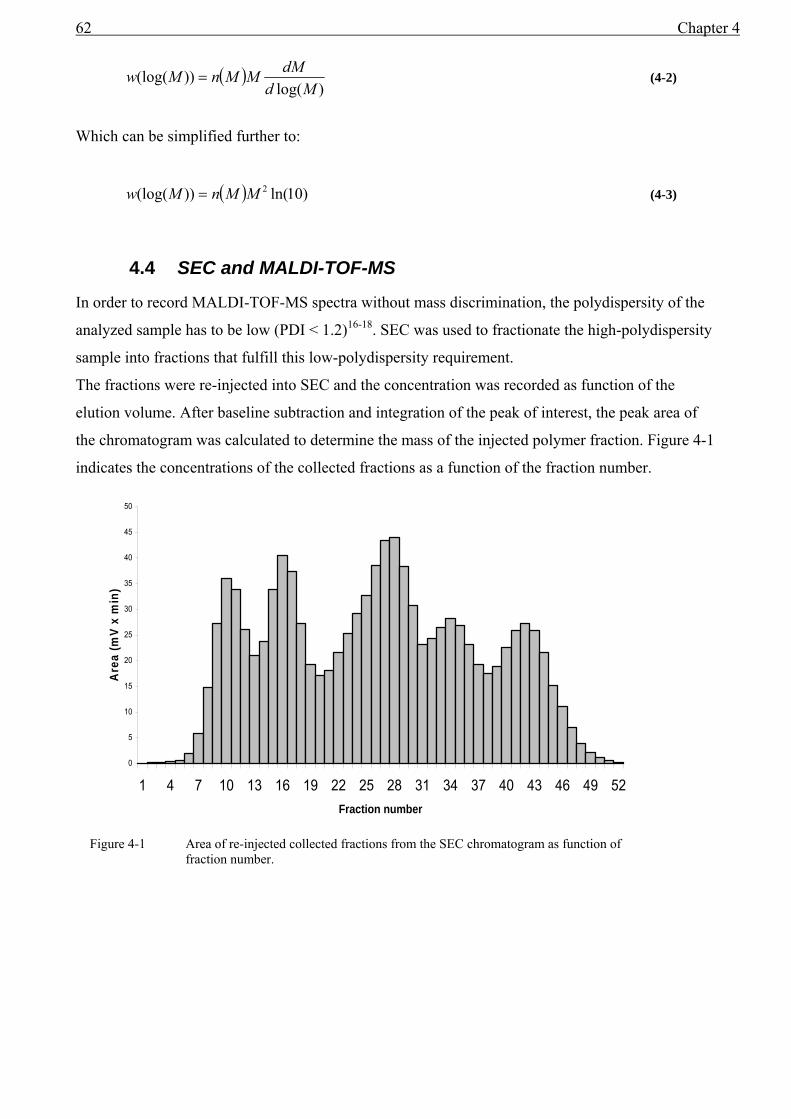
62 Chapter 4
( ))log(
))(log(Md
dMMMnMw = (4-2)
Which can be simplified further to:
( ) )10ln())(log( 2MMnMw = (4-3)
4.4 SEC and MALDI-TOF-MS
In order to record MALDI-TOF-MS spectra without mass discrimination, the polydispersity of the
analyzed sample has to be low (PDI < 1.2)16-18. SEC was used to fractionate the high-polydispersity
sample into fractions that fulfill this low-polydispersity requirement.
The fractions were re-injected into SEC and the concentration was recorded as function of the
elution volume. After baseline subtraction and integration of the peak of interest, the peak area of
the chromatogram was calculated to determine the mass of the injected polymer fraction. Figure 4-1
indicates the concentrations of the collected fractions as a function of the fraction number.
0
5
10
15
20
25
30
35
40
45
50
1 4 7 10 13 16 19 22 25 28 31 34 37 40 43 46 49 52Fraction number
Are
a (m
V x
min
)
Figure 4-1 Area of re-injected collected fractions from the SEC chromatogram as function of
fraction number.
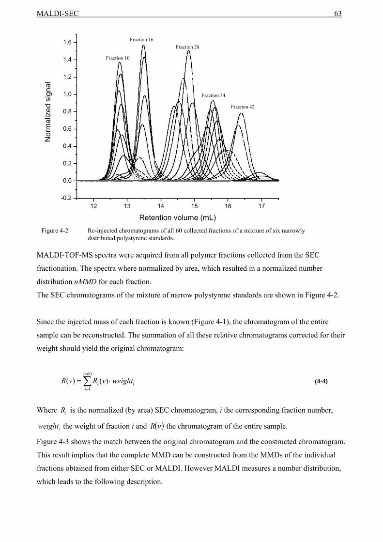
MALDI-SEC 63
MALDI-TOF-MS spectra were acquired from all polymer fractions collected from the SEC
fractionation. The spectra where normalized by area, which resulted in a normalized number
distribution nMMD for each fraction.
The SEC chromatograms of the mixture of narrow polystyrene standards are shown in Figure 4-2.
Since the injected mass of each fraction is known (Figure 4-1), the chromatogram of the entire
sample can be reconstructed. The summation of all these relative chromatograms corrected for their
weight should yield the original chromatogram:
i
i
ii weightvRvR ⋅= ∑
=
=
60
1)()( (4-4)
Where iR is the normalized (by area) SEC chromatogram, i the corresponding fraction number,
iweight the weight of fraction i and ( )vR the chromatogram of the entire sample.
Figure 4-3 shows the match between the original chromatogram and the constructed chromatogram.
This result implies that the complete MMD can be constructed from the MMDs of the individual
fractions obtained from either SEC or MALDI. However MALDI measures a number distribution,
which leads to the following description.
12 13 14 15 16 17-0.2
0.0
0.2
0.4
0.6
0.8
1.0
1.2
1.4
1.6N
orm
aliz
ed s
igna
l
Retention volume (mL) Figure 4-2 Re-injected chromatograms of all 60 collected fractions of a mixture of six narrowly
distributed polystyrene standards.
Fraction 10
Fraction 16 Fraction 28
Fraction 34
Fraction 42
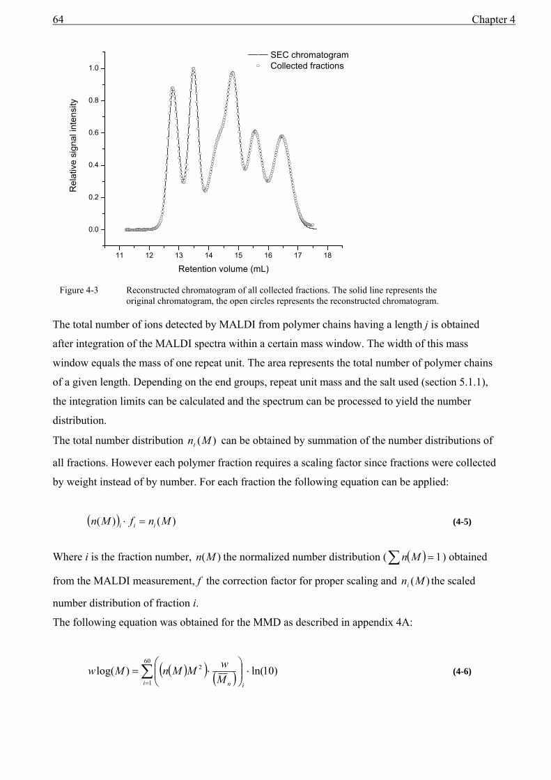
64 Chapter 4
The total number of ions detected by MALDI from polymer chains having a length j is obtained
after integration of the MALDI spectra within a certain mass window. The width of this mass
window equals the mass of one repeat unit. The area represents the total number of polymer chains
of a given length. Depending on the end groups, repeat unit mass and the salt used (section 5.1.1),
the integration limits can be calculated and the spectrum can be processed to yield the number
distribution.
The total number distribution )(Mnt can be obtained by summation of the number distributions of
all fractions. However each polymer fraction requires a scaling factor since fractions were collected
by weight instead of by number. For each fraction the following equation can be applied:
( ) )()( MnfMn iii =⋅ (4-5)
Where i is the fraction number, )(Mn the normalized number distribution ( ( ) 1=∑ Mn ) obtained
from the MALDI measurement, f the correction factor for proper scaling and )(Mni the scaled
number distribution of fraction i.
The following equation was obtained for the MMD as described in appendix 4A:
( )( ) ( ) )10ln()log(60
1
2 ⋅⎟⎟⎠
⎞⎜⎜⎝
⎛⋅= ∑
= ii nMwMMnMw (4-6)
11 12 13 14 15 16 17 18
0.0
0.2
0.4
0.6
0.8
1.0R
elat
ive
sign
al in
tens
ity
Retention volume (mL)
SEC chromatogram Collected fractions
Figure 4-3 Reconstructed chromatogram of all collected fractions. The solid line represents the
original chromatogram, the open circles represents the reconstructed chromatogram.

MALDI-SEC 65
Where w is the weight of a fraction, nM the number-average molar mass, i the fraction number and
M the molar mass. The result of computing all fractions into one MMD distribution is shown in
Figure 4-4.
Table 9 MMD moments obtained by MALDI and by other methods.
MALDI Conv.
Calibration
Univ.
Calibration
Triple
detection
Error relative#
to MALDI (%)
nM 5271 5075 5060 5165 3.2
wM 13111 13150 12850 13500 0.4
zM 23822 23500 23050 24750 0.2 # The average moment of the three calibration methods was taken to compare with MALDI.
The MMDs obtained by MALDI-TOF-MS and by SEC are plotted in Figure 4-4. The slightly shift
in the lower mass region (peak1) results in a relatively large error in the value of nM as seen in
Table 9. The values obtained by conventional calibration are closest to those obtained by MALDI.
In theory, if SEC would not suffer from column broadening, these numbers should be identical.
Since broadening mainly affects the resolution of the peaks, the area under each peak should be the
same for both distributions. A comparison of peak areas can be found in Table 10.
3.0 3.5 4.0 4.5 5.0
0.0
0.5
1.0
1.5
2.0
2.5
dw(lo
gM)/d
logM
LogM
MALDI SEC Tung
Figure 4-4 A comparison of the MMD obtained by MALDI and SEC. The MALDI signal was subjected to
broadening by Tung’s equation so that the two MMDs could be compared.
Peak 1 Peak 2 Peak 3 Peak 4 Peak 5

66 Chapter 4
Table 10 The areas of the peaks indicated in Figure 4-4.
Area MALDI Area SEC
Peak1 0.180 0.181
Peak2 0.162 0.159
Peak3 0.336 0.332
Peak4 0.170 0.171
Peak5 0.152 0.157
Total area 1.000 1.00
Table 10, confirms that a complete MMD without mass discrimination can be constructed from
MALDI-TOF-MS data of fractions obtained from SEC.
To visualize the effect of column broadening in SEC, the MMD reconstructed from the MALDI-
TOF-MS data of the fractionated sample was subjected to axial dispersion by Tung’s equation as
described in section 3.4.
( )( )
( )( ) MdMw
dvMd
MM
dvMd
Mw loglog2log
log'logexp2log
1)'(log0 2
2
2
⋅⋅
⎟⎟⎟⎟⎟
⎠
⎞
⎜⎜⎜⎜⎜
⎝
⎛
⋅⎟⎠⎞
⎜⎝⎛
−
−−
⋅⋅⎟⎠⎞
⎜⎝⎛
−⋅
= ∫∞
σπσ (4-7)
Where σ is the dispersion constant, ( )dv
Md−log the slope of the calibration curve, )'(log Mw the
apparent MMD, and )(log Mw the “true” MMD. In contrast to all methods describing the
chromatographic band broadening, the “true” MMD is not known, since it is the desired outcome of
the selected method. In this case Tung’s equation is used in the opposite way, since mass
discrimination was reduced to a minimum and the “true” MMD obtained by MALDI was used to
compute the apparent MMD.
A good fit was obtained with a constant Gaussian broadening of ( )dv
Md−
⋅logσ = 0.052. Figure 4-4
clearly shows the broadening of SEC at higher masses. The apparent MMD (Tung) is clearly
broadened too much at the lower mass tail of the lowest molar mass distribution (the lowest molar
mass standard). The observed band broadening can only be visualized if the polydispersity of the
sample is less than the observed band broadening. Especially towards the lower mass range of this
particular set of columns, the contribution of the polymer polydispersity starts to overshadow the
observed band broadening. If the polymer polydispersity dominates the observed band broadening,
than it also represents the true (continuous) molar-mass distribution. The column performance in
terms of band broadening is extensively discussed elsewhere19.
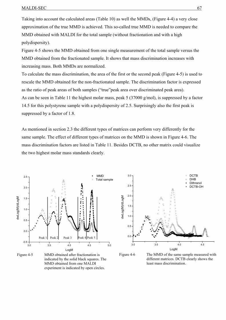
MALDI-SEC 67
Taking into account the calculated areas (Table 10) as well the MMDs, (Figure 4-4) a very close
approximation of the true MMD is achieved. This so-called true MMD is needed to compare the
MMD obtained with MALDI for the total sample (without fractionation and with a high
polydispersity).
Figure 4-5 shows the MMD obtained from one single measurement of the total sample versus the
MMD obtained from the fractionated sample. It shows that mass discrimination increases with
increasing mass. Both MMDs are normalized.
To calculate the mass discrimination, the area of the first or the second peak (Figure 4-5) is used to
rescale the MMD obtained for the non-fractionated sample. The discrimination factor is expressed
as the ratio of peak areas of both samples (“true”peak area over discriminated peak area).
As can be seen in Table 11 the highest molar mass, peak 5 (37000 g/mol), is suppressed by a factor
14.5 for this polystyrene sample with a polydispersity of 2.5. Surprisingly also the first peak is
suppressed by a factor of 1.8.
As mentioned in section 2.3 the different types of matrices can perform very differently for the
same sample. The effect of different types of matrices on the MMD is shown in Figure 4-6. The
mass discrimination factors are listed in Table 11. Besides DCTB, no other matrix could visualize
the two highest molar mass standards clearly.
Peak 1 Peak 2 Peak 3 Peak 4 Peak 5
3.0 3.5 4.0 4.5
0.0
0.5
1.0
1.5
2.0
2.5
3.0 DCTBDHBDithranolDCTB-OH
dwLo
g(M
)/dLo
gM
LogM 3.0 3.5 4.0 4.5 5.0
-0.5
0.0
0.5
1.0
1.5
2.0
2.5
dwLo
g(M
)/dLo
gM
LogM
MMDTotal sample
Figure 4-5 MMD obtained after fractionation is
indicated by the solid black squares. The MMD obtained from one MALDI experiment is indicated by open circles.
Figure 4-6 The MMD of the same sample measured with different matrices. DCTB clearly shows the least mass discrimination.

68 Chapter 4
Table 11 Discrimination factors calculated from the peak areas of Figure 4-6. for different types of matrices.
MMD area of: Mass discrimination factor
fractionated
sample
non-fractionated
sample
DCTB DHB Dithranol DCTB-OH
Peak1 0.180 0.102 1.8 1.0 1.0 1.0
Peak2 0.162 0.159 1.0 2.7 1.5 1.7
Peak3 0.336 0.181 1.8 10.4 4.7 10.5
Peak4 0.170 0.018 9.5 ∞ ∞ ∞
Peak5 0.152 0.010 14.5 ∞ ∞ ∞
Total area 1.000 0.471
4.5 Conclusions
By creating a well known, synthetic reference sample, we have been able to quantitatively access
the mass discrimination occurring in MALDI-TOF-MS analysis of polystyrene.
When MALDI-TOF-MS spectra are acquired of broad polystyrenes (PDI > 1.2) mass
discrimination does occur. The “true” MMD, without mass discrimination, could be constructed
from MALDI-TOF-MS data of fractions obtained from SEC. For polystyrene the matrix trans-2-[3-
(4-tert-Butylphenyl)-2-methyl-2-propenylidene]malononitrile reduces the mass discrimination to
less then a factor 14.5 over a broad mass range (1000 - 37000 g/mol) compared to the “true”
MMD. This makes this matrix superior to other tested matrices in terms of mass discrimination.
Mass discrimination on both the low and the high molar mass tail was observed for the broad
polystyrene standard. A possible reason for the mass discrimination on the low molar mass tail
could be detector saturation effects. A relatively high laser intensity was needed to obtain
reasonable intensities for the highest molar masses. These high laser intensities could lead to
saturation effects of the detector due to an increase of low-molar-mass species.
Polystyrene polymers larger than 10,000 g/mol can lead to agglomerates as shown in appendix 4E.
During the laser ablation, high-molar-mass species are not completely “disentangled” in the gas
phase. In general, this phenomenon alters the MMD of broad distributions and it is hard to prevent
(although dilution of the sample may help). However, this error can be safely neglected compared
to the observed mass discrimination.
SEC
Column band-broadening effects could be described very well by axial dispersion. Moreover,
within a molar mass range of 1000 - 37000 g/mol, the increase of the band broadening with
increasing molar mass could be described by a dispersion constant independent of molar mass.
The computed wM and zM of MALDI and SEC were found to be in excellent agreement. The
small deformation of the lower mass region (peak1) results in a relatively high error in the value of

MALDI-SEC 69
nM as seen in Table 9. Moreover, this effect has also already been observed in appendix 3E for the
lowest-molar-mass standard. In general, polystyrene standards of molar masses lower than 2500
g/mol show a small discrepancy between pM values given by their suppliers and observed with
MALDI.
The theoretical conversion of MALDI spectra to SEC chromatograms was confirmed by the
experiments. Note that proper baseline corrections are crucial to obtain reliable MMDs.

70 Chapter 4
Reference List 1. Tang, X.; Dreifuss, P. A.; Vertes, A. Rapid commun. Mass Spectrom. 1995, 9, 1141-1147.
2. Shimada, K.; Lusenkova, M. A.; Sato, K.; Saito, T.; Matsuyama, S.; Nakahara, H.; Kinugasa, S. Rapid commun. Mass Spectrom. 2001, 15, 277-282.
3. Schriemer, D. C.; Li, L. Anal. Chem. 1997, 69, 4169-4175.
4. Rashidzadeh, H.; Guo, B. Anal. Chem. 1998, 70, 131-135.
5. Karas, M.; Hillenkamp, F. Anal. Chem. 1988, 60 (20), 2299-2301.
6. Hanton, S. D. Chem. Rev. 2001, 101, 527-569.
7. Belu, A. M.; DeSimone, J. M.; Linton, R. W.; Lange, G. W.; Friedman, R. M. J. Am. Soc. Mass Spectrom. 1996, 7, 11-24.
8. Axelsson, J.; Scrivener, E.; Haddleton, D. M.; Derrick, P. J. Macromolecules 1996, 29, 8857-8882.
9. Hanton, S. D.; Clark, P. A.; Owens, K. G. J. Am. Soc. Mass Spectrom. 1999, 10, 104-111.
10. McEwen, C. N.; Jackson, C.; Larsen, B. S. Int. J. Mass Spectrom. Ion Phys 1997, 160, 387-394.
11. Ulmer, L.; Mattay, J.; Torres-Garcia, H. G.; Luftmann, H. European Journal of Mass Spectrometry 2000, 6 (1), 49-52.
12. Wallace, W. E.; Guttman, C. M. J. Natl. Inst. Stand. Technology 2002, 107, 1-17.
13. Guttman, C. M.; Blair, W. R.; Danis, P. O. Journal of Polymer Science PartB: Polymer Physics 1997, 35, 2409-2419.
14. Byrd, M. H. C.; McEwen, C. N. Anal. Chem. 2000, 72, 4568-4576.
15. Shortt, D. W. Journal of Liquid Chromatography 1993, 16 (16), 3371-3391.
16. Spickermann, J.; Martin, K.; Räder, H. J.; Müllen, K.; Schlaad, H.; Müller, A. H. E.; Krüger, R.-P. European Journal of Mass Spectrometry 1996, 2, 161-165.
17. Montaudo, G.; Montaudo, M.S.; Puglisi, C.; Samperi, F; Macromolecules 1995, 28, 7983-7989.
18. Montaudo, G.; Montaudo, M.S.; Puglisi, C.; Samperi, F.; Rapid commun. Mass Spectrom. 1995, 9, 453-460.
19. Popovici, S. Towards Smal and Fast Size-Exclusion Chromatography, PhD Thesis, University of Amsterdam 2004.
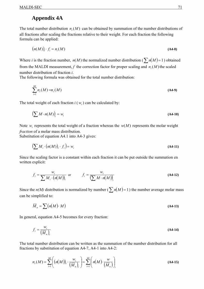
MALDI-SEC 71
Appendix 4A The total number distribution )(Mnt can be obtained by summation of the number distributions of all fractions after scaling the fractions relative to their weight. For each fraction the following formula can be applied:
( ) )()( MnfMn iii =⋅ (A4-8)
Where i is the fraction number, )(Mn the normalized number distribution ( ( ) 1=∑ Mn ) obtained from the MALDI measurement, f the correction factor for proper scaling and )(Mni the scaled number distribution of fraction i. The following formula was obtained for the total number distribution:
)()(60
1MnMn t
ii∑
=
= (A4-9)
The total weight of each fraction i ( iw ) can be calculated by:
( ) iiwMnM =⋅∑ )( (A4-10)
Note iw represents the total weight of a fraction whereas the )(Mw represents the molar weight fraction of a molar mass distribution. Substitution of equation A4.1 into A4-3 gives:
( )( ) iiii wfMnM =⋅⋅∑ )( (A4-11)
Since the scaling factor is a constant within each fraction it can be put outside the summation en written explicit:
( )( )∑ ⋅=
ii
ii MnM
wf or ( )( )
i
ii MnM
wf
∑ ⋅= (A4-12)
Since the n(M) distribution is normalized by number ( ( ) 1=∑ Mn ) the number average molar mass can be simplified to:
( )( )∑ ⋅= MMnM n (A4-13)
In general, equation A4-5 becomes for every fraction:
( )in
ii M
wf = (A4-14)
The total number distribution can be written as the summation of the number distribution for all fractions by substitution of equation A4-7, A4-1 into A4-2:
( )( ) ( ) ( ) ( )ii ni in
iit M
wMnMw
MnMn ∑∑==
⎟⎟⎠
⎞⎜⎜⎝
⎛⋅=⎟⎟
⎠
⎞⎜⎜⎝
⎛⋅=
60
1
60
1)( (A4-15)

72 Chapter 4
The logarithmic molar mass distribution can be obtained after substitution of equation A4-8 into equation 4.3 (see section 4.2.1):
( )( ) ( ) )10ln()log(60
1
2 ⋅⎟⎟⎠
⎞⎜⎜⎝
⎛⋅= ∑
= ii nMwMMnMw (A4-16)
This equation can also be written in terms of molar weight fractions:
( )( ) )10ln()log(60
1⋅⋅= ∑
=iiwMwMw (A4-17)
The advantage of equation A4-9 is that all terms are still expressed as number distributions as measured directly by the MALDI. Appendix 4B The MALDI-TOF-MS raw data spectra of a mix of six narrow polystyrene standards measured with different matrixes.
% Intensity
999 9799 18599 27399 36199 45000
Mass (m/z)
DCTB
9990
9799 18599 27399 36199 45000
Dithranol
9990
9799 18599 27399 36199 450000
DHB
9990
9799 18599 27399 36199 45000
% Intensity
% Intensity
% Intensity
DCTB-OH

MALDI-SEC 73
Appendix 4C The polydispersity of each fractionated polymer sample of a mixture of six narrow polystyrene standards. Fraction
nr. D
(Mw/Mn) File
name D
(Mw/Mn)Fraction
nr. D
(Mw/Mn)PS2_01 1.02 PS2_21 1.06 PS2_41 1.04 PS2_02 1.02 PS2_22 1.05 PS2_42 1.04 PS2_03 1.01 PS2_23 1.04 PS2_43 1.04 PS2_04 1.09 PS2_24 1.04 PS2_44 1.04 PS2_05 1.04 PS2_25 1.04 PS2_45 1.04 PS2_06 1.03 PS2_26 1.03 PS2_46 1.04 PS2_07 1.03 PS2_27 1.03 PS2_47 1.04 PS2_08 1.02 PS2_28 1.03 PS2_48 1.04 PS2_09 1.03 PS2_29 1.03 PS2_49 1.05 PS2_10 1.02 PS2_30 1.04 PS2_50 1.05 PS2_11 1.03 PS2_31 1.06 PS2_51 1.05 PS2_12 1.04 PS2_32 1.05 PS2_52 1.03 PS2_13 1.06 PS2_33 1.05 PS2_53 -# PS2_14 1.07 PS2_34 1.04 PS2_54 -# PS2_15 1.04 PS2_35 1.04 PS2_55 -# PS2_16 1.03 PS2_36 1.04 PS2_56 -# PS2_17 1.03 PS2_37 1.05 PS2_57 -# PS2_18 1.03 PS2_38 1.06 PS2_58 -# PS2_19 1.05 PS2_39 1.06 PS2_59 -# PS2_20 1.08 PS2_40 1.05 PS2_60 -#
# Fractions 53 through 60 did not yield a significant response due to the low amount of material present. Appendix 4D The MMD obtained by conventional calibration, universal calibration and light scattering.
2.5 3.0 3.5 4.0 4.5 5.0
0.0
0.2
0.4
0.6
0.8
1.0
1.2
1.4
dw(L
ogM
)/d(L
ogM
)
LogM(g/mol)
Universal calibration Light scattering Conventional calibration

74 Chapter 4
Appendix 4E The MALDI spectrum of the well defined broad polystyrene standard consisting of six narrow standards.
All six peaks of the individual standards are marked. Note that peak four merged together with peak three and is much broader in terms of chain numbers resulting in a broader peak, where the individual peak maximum of the fourth standard is no longer observed. The formation of agglomerates is also observed i.e. peak three and peak five (5+3). Even the combination of peak five and peak six was observed (not shown). Although multiple peak formation leads to biased molar mass distribution, the effects are rather weak in terms of intensity.
1316.0 11052.8 20789.6 30526.4 40263.2Mass (m/z)
50
100
% Intensity
1
2
3
4
5
6 5+3 6+3
MALDI of homopolymers 75
Chapter 5
5 MALDI of homopolymers
5.1 Introduction
MALDI-TOF-MS spectra of homopolymers contain information on end groups and molar-mass
distributions. Unfortunately this information is not the direct outcome of the analysis and, hence,
mathematical operations are needed. We developed software based on the definitions described in
the next paragraph to extract information from spectra. Since this chapter only deals with
homopolymers we will add some definitions for copolymers in chapter 6.
5.2 Definitions
5.2.1 Determination of numbers of repeat units and end-group masses
The observed mass of a singly charged copolymer chain in MALDI-TOF-MS is described by the
following equation:
21 endendionAAobs mmmnrmm +++⋅= (5.1)
where obsm is the observed mass of a peak in the MALDI-TOF-MS spectrum, Am is the mass of the
repeat unit, Anr is the number of repeat units, ionm the mass of the adduct ion and 1endm , 2endm are
the masses of the end groups. The total end-group mass ( )21 endend mm + can be calculated from the
above equation as long as the number of repeat units and the adduct mass are known (normally the
adduct-ion mass is known, since salt is added for the analysis). However, for a given peak mass we
do not know how many repeat units are present.

76 Chapter 5
Let there be two polymers, one with two identical end groups, the mass of which equals 2/3 of the
mass of a repeat unit, and the second polymer has one end group with a mass equal to 2/3 of the
mass of a repeat unit, whereas the mass of the other end group equals 5/3 of the mass of a repeat
unit (see Figure 5-1).
The total masses of both schematic polymer chains are identical;
( )( ) ( ) AA mm 6323573/22 ++=+⋅ , although the end-group mass and the number of repeat units
for both polymer chains are different. As a consequence, the solutions for the end group mass
become a function of the number of repeat units. Therefore we define the residual mass ( )resm as
being the minimum total end-group mass, and the corresponding maximum number of repeat
units ( )MaxAnr _ :
ionMaxAAobsres mnrmmm −⋅−= _ (5.2)
⎟⎟⎠
⎞⎜⎜⎝
⎛ −=
A
ionobsMaxA m
mmINTnr _ (5.3)
Note that the resm of both chains in Figure 5-1 would be Am⋅31 and the maximum number of
repeat units 8.
The solutions for the total end-group masses for a singly charged peak in a MALDI-TOF-MS
spectrum can now be written in a more general form:
( ) nmmm Aresnend ⋅+= (5.4)
Where ( )nendm represents all the solutions for the total end-group masses for a given residual mass,
n equals the maximum number of times one repeat unit mass would “fit” within the total end groups
(e.g. an end-group mass of 154 amu can be considered as one repeat unit of styrene (104 amu) and
an resm of 50), or in other words where n is the smallest integer part of the ratio Aend mm .
Figure 5-1 Schematic polymer chains having different end-group masses and different numbers of repeat units, but the same overall molar mass.
= Am⋅32
= Am
= end group
= repeat unit = Am⋅35

MALDI of homopolymers 77
5.2.2 End-group Correlation Function (ECF)
We just defined a method to calculate for each peak all possible total end group masses. However,
since most polymers only have few different end groups, only one peak of each series should be
sufficient to determine the end-group masses. Figure 5-2 shows a typical MALDI-TOF-MS
spectrum of a homopolymer of styrene with two series of peaks having different total end-group
masses.
To obtain the highest possible precision for end-group analysis with MALDI-TOF-MS, we
introduce the End-group Correlation Function (ECF). This function finds the maximum correlation
of a given end-group mass along the entire spectrum.
( )( )end A A ion endECF m I m nr m m= ⋅ + +∑ (5.5)
Where I is the corresponding intensity of the spectrum at a given mass, and ( )endECF m the end-
group correlation at any given end-group mass.
Note that while calculating the ECF as a function of the end-group mass, the upper value of endm
must be selected at least equal to the mass of a repeat unit in order to find all end-group masses. The
mass step-size of endm is set the same as the maximum mass difference between two consecutive
data points (normally at the end of the spectrum since the data is acquired in the time domain). The
result of a calculated ECF is shown in Figure 5-3.
788.0 1216.8 1645.6 2074.4 2503.2 2932.0
104.1
104.1
788.0 1216.8 1645.6 2074.4 2503.2 2932.0
104.1
104.1
Inte
nsity
(%)
Mass (amu) Figure 5-2 A MALDI-TOF-MS spectrum of polystyrene, reflective positive-ion mode, DCTB as
matrix and Ag+ as a cationization agent. The two different series of peaks differ by 104.1 amu, the mass of one repeat unit of styrene.

78 Chapter 5
The repeat unit mass of polystyrene equals 104.1 amu therefore all peaks below 104.1 amu must be
different end groups. Figure 5-3 shows the existence of two well resolved peak clusters at 13.2, 58.2
amu respectively. The clusters present the “average-isotopic” distributions, since the shape of the
isotopic distributions slightly changes along the molar-mass scale, which affects the accuracy of the
end group mass. Figure 5-4 shows a change in peak-maximum-average repeat mass of less then 0.1
amu. The peak maximum is defined as the corresponding mass of the most abundant peak within
the isotope cluster of a given number of repeat units. The average mass of a repeat unit is calculated
by the corresponding mass of the peak maximum divided by the number of repeat units resulting in
the peak-maximum-average repeat mass.
According to equation (5.2) the accuracy of resm depends on the product of _A A Maxm nr⋅ . The
deviation between the value of the peak-maximum-average repeat mass and the average mass of the
monomer decreases with an increase of the number of repeat units resulting in saw-toothed function
of _A A Maxm nr⋅ (the absolute error of resm ) versus number of repeat units (see Figure 5-4). The end-
group calculation must be applied to the entire mass range to obtain accurate end-group masses. As
long as a mass range of at least 11 repeat units are used to compute the end-group masses, the
obtained deviation is between -0.6 amu and -0.4 amu for polystyrene. It is more convenient to shift
the end-group masses by 0.5 amu resulting in a deviation of ±0.1 amu. The ECF functions shown is
this thesis are already corrected for the deviation depending on the mass range and the type of
polymer. Besides such a correction, the spectrum typically deviates by 0.5 amu using the instrument
default calibration.
The two peaks at 13.2 and 58.2 amu (Figure 5-3) are the residual masses for the end groups of the
spectrum in Figure 5-2. The general solutions for the end groups become:
( )1 13.2end Am m n= + ⋅ and ( )258.2end Am m n= + ⋅ (5.6)
Figure 5-3 The result of the calculation of the end-group correlation function (arbitrary units) of a polystyrene sample (Figure 5-2).
endm (amu)
ECF
24 49 74 99 124
13.2 58.2
117.2

MALDI of homopolymers 79
An experienced user of the MALDI would have noticed immediately the difference in the isotopic
patterns of Figure 5-2 (not visible). This is also noticed in Figure 5-3. Before starting to assign the
other end group, it is wise to check whether all species are charged with the same cation. Preparing
the sample with a different salt should yield all species shifted in the same manner. The expert user
would recognize a mass difference close to 44 as the difference between Ag and Cu. A small trace
of a copper salt turned out to be the cause of the “second end group” in the present case. This
example underlines the need to verify whether all species are ionized by the same cation.
In some cases a higher accuracy is needed and equation (5.5) needs to be modified and needs as
input the repeat mass and an approximation of the end-group mass. The repeat mass can be obtained
by the Auto Correlation Function (ACF) discussed in the next section, whereas the approximated
end-group mass is obtained by equation (5.5).
( )( )( )
( )( )
A A
A
IMax nr m
HR end endIMax nr
ECF m I m IMax m+⎛ ⎞
= +⎜ ⎟⎝ ⎠
∑ ∑ (5.7)
Where HRECF is the high resolution end group determination, ( )IMaxm the corresponding mass of
the maximum intensity within the isotopic cluster at a given number of repeat units. Note that the
endm must be lower then the mass of a repeat unit in contrast to equation (5.5).

80 Chapter 5
5.2.3 Auto-Correlation Function (ACF)
The last part of this section deals with the determination of the repeat-unit mass ( )Am or the
identification of the monomer used in the polymerization. Figure 5-5 shows a spectrum of a
polymer with four different end groups. Although the repeat mass is the same as in Figure 5-2 this
is not immediately clear from the spectrum.
0 50 100 150 200 250
104.06
104.08
104.10
104.12
104.14pe
ak-m
ax-a
vera
ge re
peat
mas
s (a
mu)
number of repeat units polystyrene
Figure 5-4 The peak-maximum-average repeat mass is the most abundant peak in an isotopic cluster divided by the number of repeat units. The dashed line is the average molar mass of the repeat units. The graph demonstrates the mass shift of repeat unit mass if only the most abundant peak of an isotopic distribution is taken into account.
The insert shows the saw-toothed function of the absolute error of the end-group mass versus the number of repeat units.
0 50 100 150 200 2500.2
0.0
-0.2
-0.4
-0.6
-0.8
-1.0
abso
lute
erro
r of t
he e
nd-g
roup
mas
s
number of repeat units of polystyrene
In
tens
ity (%
)
Figure 5-5 A MALDI-TOF-MS spectrum of polystyrene with four distinct series of peaks with a mass increment of 104.1 amu, the mass of one repeat unit styrene.
100
773 1316 1859 2402 2945 3488
104.1
104.1
Mass (amu)
104.1 104.1

MALDI of homopolymers 81
The auto-correlation function2 (ACF) returns the maximum correlation for any chosen repeat unit
mass, in this case the maximum correlation is found at a mass difference of 104.1, 208.2, 312.3…
etc. (see Figure 5-6).
( )2)(
)()()(
∑∑∑ +⋅
=mI
mmImImACF rep
rep (5.8)
Where repm , the mass step-size, is set equal to the maximum mass difference between two
consecutive data points. The observed mass difference of 104.1 amu corresponds to the mass of a
styrene repeat unit.
The ACF does not return the exact average mass of a repeat unit but the “local” average repeat mass
in the mass range of interest. The problem is similar to the peak-maximum-average-repeat mass
(see Figure 5-4). As a consequence, the ACF will always return a slightly lower repeat-unit mass
compared to the exact average repeat-unit mass. All deviations are typically below 0.1 amu and
decrease with increasing mass. Note that these minor deviations do not hamper the identification of
the monomer used in the polymerization.
5.2.4 Conclusion
The aim of the concepts described above is to obtain a user-independent method for the
interpretation of MALDI-TOF-MS spectra. In summary:
• ACF reveals the repeat mass ( )Am , which suggests the polymer identity. Isomers cannot be
distinguished based on mass.
• ECF reveals the number of different end-group combinations and the corresponding residual
masses ( )resm .
100
A
CF
Figure 5-6 The result of the auto-correlation function for a polymer with a repeat unit mass of 104.1 amu which corresponds with the mass of a styrene repeat unit.
repm (amu)
0 80 160 240 320 400
208.2104.1
312.3

82 Chapter 5
The generic solution, equation (5.4), is obtained for each total end-group mass from one MALDI-
TOF-MS spectrum. However, for each polymeric series only one of these values for the total end-
group mass is correct. At this point chemistry and mathematics must come together. Chemical
information is needed to reduce the number of possible solutions for the end-group masses. The
next section will demonstrate the need for both mathematics and chemistry. In order to demonstrate
the use of the previously derived equations, the data will be analyzed first in the conventional way
(only taking a limited region of the entire spectrum and trying to explain every peak).
5.3 End-group analysis with MALDI-TOF-MS to reveal the initiator
functionality
5.3.1 Introduction
Control Radical Polymerization (CRP) enables synthesis of complex architectures (gradient, block,
graft, ect.). The three most effective methods of CPR include Nitroxide Mediated Polymerization
(NMP), atom-transfer radical polymerization (ATRP) and Reversible Atom Fragmentation Transfer
(RAFT) polymerization3,4. Restricting our discussion to the ATRP of methyl methacrylate (MMA),
it has been observed that multifunctional halides, such as trichloroalkanes, successfully initiate the
polymerization of MMA via ATRP5. However, there is no direct measurement for the initiator
functionality (mono-, di-, or trifunctional in the case of trichloroalkanes). It is well known that the
initiation of the ATRP process largely determines the overall control achieved during the
polymerization.
Polymer-end-group analysis is an effective way to establish the initiation mechanism of functional
halide initiators. In recent years, MALDI-TOF-MS has been employed as an effective tool from
characterization of polymers, obtained via controlled radical polymerization, clearly giving insight
into comonomer incorporation, end-group assignment etc. Recently published article gives an
excellent review of the use of soft-ionization techniques such as ESI and MALD-TOF-MS for the
analysis of polymers. MALDI-TOF-MS is an effective technique for end-group analysis. However,
in MALDI the presence of weak carbon-halogen bonds leads to fragmentation despite the soft
nature of MALDI. This results in poorly resolved spectra6,7 and affects the accuracy of the end-
group analysis,.
In this study, polymer samples were thermally treated prior to MALDI-TOF-MS analysis to obtain
high-resolution spectra. This allows the determination of the true initiator functionality of 2,2,2-
trichloroethanol (TCE).
Experimental
A typical polymerization was carried out in a 50-mL three-neck round-bottom flask. p-Xylene
(11.05 g, 0.10 mol), MMA (2.42 g, 0.02 mol), CuCl (0.037 g, 0.4 mmol), and CuCl2 (0.003 g, 0.02
MALDI of homopolymers 83
mmol) were accurately weighed and transferred to the flask. The ligand, N,N,N′,N″,N″-
pentamethyldiethylenetriamine (PMDETA) (0.07 g, 0.4 mmol) was then added. After the reaction
mixture was purged with argon for 30 min, the flask was immersed in a thermostated oil bath,
maintained at 90 ºC, and stirred for 10 min. A light green, slightly heterogeneous reaction mixture
was obtained. The initiator, TCE (0.15 g, 0.10 mL, 1.00 mmol) was added slowly using a degassed
syringe. The reactions were carried out under an argon atmosphere. Samples were withdrawn at
suitable time periods throughout the polymerization. Pre-determined amounts of the sample were
transferred immediately after withdrawal into GC vials and diluted with 1,4-dioxane, to
subsequently determine the monomer conversion using GC. The remaining sample was diluted with
THF and passed through a column packed with aluminum oxide prior to SEC and MALDI-TOF-
MS measurements.
Materials
Methyl methacrylate (MMA, 99+%) was distilled and stored over molecular sieves at -15°C. p-
Xylene (99+% HPLC grade Aldrich, Zwijndrecht the netherlands) was stored over molecular sieves
and used without futher purification. N,N,N′,N″,N″-pentamethyldiethylenetriamine (PMDETA,
Aldrich 99%), 2,2,2-trichloroethanol (TCE, Aldrich, 99%), p-toluenesulphonyl chloride (pTsCl,
Aldrich, 99%), copper (I) bromide (CuBr, Aldrich, 98%), copper (II) bromide (CuBr2, Aldrich,
99%), copper (I) chloride (CuCl, Aldrich, 98%), copper (II) chloride (CuCl2, Aldrich, 98%),
aluminum oxide (activated, basic, for column chromatography, 50-200 µm), tetrahydrofuran (THF,
Biosolve, Valkenswaard, the Nederlands), ethyl 2-bromoisobutyrate initiator (EBriB, Aldrich,
99%), and 1,4-dioxane (Aldrich, AR-grade) were used as supplied. The ligand N-npentyl-2-
pyridylmethanimine (PPI) was synthesized as described by Haddleton et al8. and distilled prior to
use.
MALDI-TOF-MS instrument
MALDI-TOF-MS measurements were performed on a Voyager-DE-STR (Applied Biosystems,
Framingham, MA, USA) instrument equipped with a 337nm nitrogen laser. All spectra were
acquired in the positive-ion reflectron mode. Trans-2-[3-(4-tert-butylphenyl)-2-methyl-2-
propenylidene]malononitrile (DCTB) was used as matrix. Sodium trifluoracetate (Aldrich, 98%)
was added as the cationic ionization agent (approximately 1 mg/mL dissolved in THF). The matrix
was dissolved in THF at a concentration of 40 mg/mL. The dissolved-polymer concentration was
approximately 1 mg/mL. In a typical MALDI experiment, the matrix, salt and polymer solutions
were premixed in the ratio: 5 µL sample: 5 µL matrix: 0.5 µL salt. Approximately 0.5 µL of the
obtained mixture were hand spotted on the target plate. For each spectrum 1000 laser shots were
accumulated.

84 Chapter 5
Fourier-Transform Infrared Spectroscopy (FTIR)
The FTIR spectra were recorded with a BioRad Excalibur 3000 series spectrometer. One hundred
scans at a resolution of 4 cm-1 were signal-averaged, and the BioRad Merlin software was used to
analyze the spectra. Samples were prepared by casting films from a dilute polymer solution on KBr
discs for FTIR measurements. These films were thin enough to be within the range where the
Lambert-Beer law could be applied.
Results and discussion
MMA was polymerized by ATRP using EBriB, p-TsCl, or TCE as initiator. The characteristics of
the experiments are summarized in Table 12.
In Figure 5-7, the FTIR spectrum of PMMA with bromine end groups is shown after heating
overnight at different temperatures. The carbonyl band is clearly visible at 1730 cm-1 regardless of
the temperature at which the sample was treated. Upon increasing the temperature to 140 – 160 ºC a
slight shoulder is developing at 1782 cm-1. This shoulder is tentatively assigned to the formation of
a lactone at the chain end. It was particularly significant at temperatures in the range of 140 –
160ºC.
MALDI-TOF-MS is known as a soft ionization technique. However, it has been reported that
polymers with halogen end groups can fragment during the measurements7,9, due to the weakness of
the carbon-halogen bond. One of the possible side reactions in the specific case of PMMA is the
formation of lactones. This lactone formation during the measurements lowers the resolution, and
complicates the interpretation of the MALDI-TOF-MS spectra. The reduction in resolution is the
result of fragmentation during the laser ablation and/or during the time of flight. Molecules that
fragment in the flight tube will have the proper kinetic energy and arrive at the correct time in the
linear mode. In the reflector mode, these ions are reaccelerated with the mass of the charged
fragment and arrive at the wrong time, leading to spectral differences between the linear and the
reflector modes.
Table 12 Homopolymerization of MMA (ATRP) Entry Initiator Reaction time (min) Conversion (%) Molar mass (g/mol) PDI
1 pTsCla,b 230 74.0 7.1 ×10³ 1.08
2 TCEa,b 180 45.0 2.8 ×10³ 1.25
3 EBriBc,b 240 85.0 5.1×10³ 1.22
a) Target nM =5000 g/mol; [Initiator]:[CuCl]:[PMDETA] = 1:0.5:0.5, reaction temperature = 90°C. b) Volume (p-xylene)/(monomer) = 1/0.5 c) Target nM =6000 g/mol; [Initiator]:[CuBr]:[ PPI] = 1:1:2, reaction temperature = 90°C.

MALDI of homopolymers 85
In the present study the problem of reduced resolution in MALDI-TOF-MS was solved by heating
samples overnight at 150ºC, resulting in quantitative formation of the chain-end lactones. FTIR
spectroscopy was used to monitor the formation of lactones as a function of temperature.
p-toluene sulphonyl chloride (p-TsCl)
The use of p-TsCl as intiator leads to chlorine-end-functionalized PMMA (PMMA-p-TsCl). Figure
5-9a and Figure 5-9b show the MALDI-TOF-MS spectra of the PMMA-pTsCl before and after
heating, respectively. Figure 5-9c shows the theoretical spectra of the proposed structures A, B and
C (Figure 5-8).
The presence of three peaks (denoted A, B and C) indicates the existence of polymer chains with
three different end groups. The peaks at lower mass carry the same respective end groups, but
contain a smaller number of MMA repeat units. Compared to untreated PMMA, the heat-treated
PMMA shows an increased resolution within peaks B and C, whereas the resolution within peak A
remains the same. No conclusion can be drawn from the relative changes in intensities of peaks A
and C before and after heating, since MALDI-TOF-MS is not a quantitative technique.
1680 1760 1840
0.0
0.4
0.8
Rel
ativ
e in
tens
ity
Wavenumber (cm-1)
Figure 5-7 The FTIR spectra of bromine-end-functional PMMA (initiated with EBriB) as a function of temperature. The shoulder at 1782 cm-1 is enlarged to show the increase with temperature.
150-170°C 130-150°C
50-130°C
4x

86 Chapter 5
The peaks assigned to structure A corresponds to a PMMA chains with a chlorine end group. The
peak assigned to structure B corresponds to a polymer chain that has lost HCl. The peak assigned to
structure C corresponds to a polymer chain with a lactone end group, formed upon the loss of
CH3Cl. All peaks show excellent agreement between the observed and theoretical masses.
From the above spectra it is evident that thermal treatment increases the resolution. The more-
accurate masses and isotope patterns simplify the interpretation of MALDI-TOF-MS spectra of
fragmenting polymers, since the shape of the isotopic pattern is related to the number of chlorine
atoms present. The masses of polymer fragments are slightly biased towards higher masses, due to
fragmentation as discussed in section 2.1.3 and at the beginning of this section.
Despite the observed fragmentation, the spectra obtained for PMMA-pTsCl polymers are relatively
simple. Polymers with more than one chlorine atom are more challenging.
CH3
SO
O CH3
O
CH3
O
CH3
O
CH3
O61
K+CH3
SO
OCl
CH3
O
CH3
O62
K+ K+CH3
SO
O CH3
O
CH3
O OO
CH3
CH3
O
O
CH361
Figure 5-8 Different proposed structures for the observed peaks of PMMA-pTsCl. The theoretical isotope patterns
are depicted in Figure 5-9c.
A= B= C=
Figure 5-9 Figures (a) and (b) show the MALDI-TOF-MS spectra of the PMMA-pTsCl before and after heating, respectively. Figure (c) shows the theoretical spectra of the proposed structures A,B and C (Figure 5-8).
a)
6223 6269 6315 6361 6407 6454Mass (m/z)
50
100 6386.6 6286.6
6400.7 6301.6 6437.76336.66236.5
% Intensity
After heating 6223.0 6269.2 6315.4 6361. 6407. 6454.Mass (m/z)
50
100 % Intensity
Before heating 6336.3 6236.2 6436.3
6300.3 6400.4 6288.0 6388.1
Mass (m/z)
100
6223 6269 6315 6361 6407 6454
% Intensity
b)
c) 6436.2 6400.2 6386.2
C B A
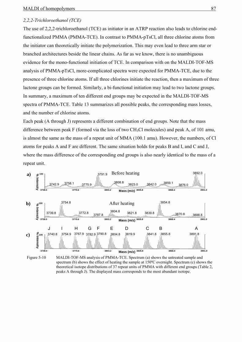
MALDI of homopolymers 87
2,2,2-Trichloroethanol (TCE)
The use of 2,2,2-trichloroethanol (TCE) as initiator in an ATRP reaction also leads to chlorine end-
functionalized PMMA (PMMA-TCE). In contrast to PMMA-pTsCl, all three chlorine atoms from
the initiator can theoretically initiate the polymerization. This may even lead to three arm star or
branched architectures beside the linear chains. As far as we know, there is no unambiguous
evidence for the mono-functional initiation of TCE. In comparison with on the MALDI-TOF-MS
analysis of PMMA-pTsCl, more-complicated spectra were expected for PMMA-TCE, due to the
presence of three chlorine atoms. If all three chlorines initiate the reaction, then a maximum of three
lactone groups can be formed. Similarly, a bi-functional initiation may lead to two lactone groups.
In summary, a maximum of ten different end groups may be expected in the MALDI-TOF-MS
spectra of PMMA-TCE. Table 13 summarizes all possible peaks, the corresponding mass losses,
and the number of chlorine atoms.
Each peak (A through J) represents a different combination of end groups. Note that the mass
difference between peak F (formed via the loss of two CH3Cl molecules) and peak A, of 101 amu,
is almost the same as the mass of a repeat unit of MMA (100.1 amu). However, the numbers, of Cl
atoms for peaks A and F are different. The same situation holds for peaks B and I, and C and J,
where the mass difference of the corresponding end groups is also nearly identical to the mass of a
repeat unit.
Figure 5-10 MALDI-TOF-MS analysis of PMMA-TCE. Spectrum (a) shows the untreated sample and spectrum (b) shows the effect of heating the sample at 150ºC overnight. Spectrum (c) shows the theoretical isotope distributions of 37 repeat units of PMMA with different end groups (Table 2, peaks A through J). The displayed mass corresponds to the most abundant isotope.
3738.0 3770.6 3803.2 3835.8 3868.4 3901.0Mass (m/z)
100 Before heating 3892.03791.9
3808.8 3859.1 3758.13742.9 3842.03775.9 3876.0 3823.0
% Intensity
3738.0 3770.6 3803.2 3835.8 3868.4 3901.0
100 3754.8 3854.8
3804.8 3772.8 3870.8 3821.8 3839.8 3739.8 3888.8 3787.8
After heating % Intensity
Mass (m/z)
a)
b)
3738.0 3770.6 3803.2 3835.8 3868.4 3901.0
100
3855.8 3891.8 3841.83754.9 3819.9 3740.8 3804.8 3782.9 3790.83767.9 A BCDEF G H I J %
Intensity
Mass (m/z)
c)

88 Chapter 5
Figure 5-10a and Figure 5-10b show the spectra of PMMA-TCE before and after heating. The most-
relevant proposed structures can be found in appendix 5A. For each peak (A through J) the
theoretical isotope pattern is shown in Figure 5-11c.
In the spectrum of the sample before heat treatment (Figure 5-10a), only one peak shows sufficient
resolution to allow unambiguous assignment. The observed isotope pattern of the peak at 3892.0
amu (Figure 5-10a) is compared with the theoretical isotope patterns of peaks A and F (Figure 5-10c).
Based on the width of the isotope pattern it is concluded that the peak at 3892.0 amu should be
assigned to structure A (appendix 5A). A general observation is that the width of the isotope pattern
increases with the number of chlorine atoms due to the chorine isotopes (Cl35 and Cl37 with
corresponding intensity 1:0.32). The peak at 3791.9 amu (Figure 5-10a) is assigned to a chain with
identical end groups as that at 3892.0 amu, but with one MMA repeat unit less incorporated. No
further attempts were made to identify the remaining peaks due to a lack of resolution.
Table 13 All possible structures sorted by increasing mass loss relative to peak A. The fourth column refers to
the number of Cl atoms present in the polymer.
Peak Fragment# mass loss (amu) Description Cl atoms present End group mass (amu)
A - 0.0 - 3 149.40
B -(HCl) 36.5 HCl 2 112.94
C -(CH3Cl) 50.5 1 Lactone 2 98.90
D -2(HCl) 72.9 2HCl 1 76.48
E -( CH3Cl)(HCl) 86.9 1 Lactone+HCl 1 62.46
F -2(CH3Cl) 101.0 2 Lactones 1 48.43
G -3(HCl) 109.4 3HCl 0 40.02
H -2(CH3Cl) 123.4 1 Lactones+2HCl 0 25.99
I -2(CH3Cl)HCl 137.4 2 Lactones+HCl 0 11.97
J -3(CH3Cl) 151.5 3 Lactones 0 98.06 # The loss of a CH3Cl group corresponds with a formation of a lactone.
3350 3360
3354.73350 3360
3355.63350 3360
3354.6
3350 3360
3354.73350 3360
3355.63350 3360
3354.6
3350 3360
3354.73350 3360
3355.63350 3360
3354.6
3350 3360
3354.73350 3360
3355.63350 3360
3354.6
3850 3860
3854.93850 3860
3855.93850 3860
3854.8
3850 3860
3854.93850 3860
3855.93850 3860
3854.8
3850 3860
3854.93850 3860
3855.93850 3860
3854.8
3850 3860
3854.93850 3860
3855.93850 3860
3854.8
4350 4360
4355.24350 4360
4356.14350 4360
4355.0
4350 4360
4355.24350 4360
4356.14350 4360
4355.0
4350 4360
4355.24350 4360
4356.14350 4360
4355.0
4350 4360
4355.24350 4360
4356.14350 4360
4355.0
Figure 5-11 The upper trace shows enlarged parts of the spectrum at different mass intervals. The middle and lower
trace show the corresponding theoretical isotope patterns of structures B and I, respectively.
The spectra of PMMA-TCE. The theoretical spectra of structure B. The theoretical spectra of structure I.

MALDI of homopolymers 89
At this point it is not possible to deduce the initiator functionality from the MALDI-TOF-MS
analysis (Figure 5-10a), since isomeric structures may result from initiation by TCE as shown in
Figure 5-13. For obvious reasons, these structures can not be distinguished by mass spectrometry.The
spectrum of the heat-treated sample (Figure 5-13b) shows the most abundant peaks at 3754.8,
3854.8 etc., which can be assigned to either peak B or peak I. The lack of a broad isotope pattern
indicates the absence of chlorine atoms. Therefore, structure I was assigned to masses 3854.8 and
3754.8. Probably the most convincing evidence for this assignment is shown in Figure 5-11. Three
expansions of the mass spectrum are shown that are related to identical end groups at different
chain length. The experimental spectrum consistently shows the third isotopic peak as the most
abundant one. This feature is recognized in structure I whereas structure B shows the fourth peak to
be the most abundant.
The last situation in which an observed mass can be assigned to two different end groups, which
differ by nearly the mass of a repeat unit concerns peaks C and J.
The low intensity of the observed peaks 3739.5, 3839.8 etc. (Figure 5-10b) does not allow us to
judge which isotope pattern (C or J) should be assigned to these peaks. However, we know that
upon thermal treatment the vast majority of (chain end) chlorine atoms are converted to lactones,
which leads to a significant increase in the intensity of the peaks, as seen in the heat-treated
PMMA-pTsCl. Since peak I, which corresponds to the formation of two lactones, is the most
abundant peak after heat treatment, we can rule out the existence of structure J. Structure J
represents trifunctional initiation, which would result in three Cl end groups, and, therefore, in three
lactones as the dominant peak after heat treatment.
In case of the presence of a small amount of trifunctional initiator, the peak assignment of the
structures C and J cannot be made based on mass. However, the relative end-group intensities of
structure J (the formation of three lactones) should show a different relationship across the molar
mass range (a higher functionality leads in this case to a higher molar mass) compared to the other
functional initiators, since structure J is the only structure that can be obtained upon heat treatment
after trifunctional initiation. Figure 5-12 shows an overlay of the relative intensities of all relevant
structures versus the molar mass. The similar behavior of all peaks indicates the presence of one
type of initiator functionality. Note that small amounts of trifunctional initiators do not lead to a
significant increase in the polydispersity measured by SEC.
The peaks at 3739.8, 3839.8 etc. are assigned to structure C. At this point all the peaks with two
possible structures are assigned (C and J, A and F, and B and I). Peak A (3892.0) completely
disappears during heat treatment, indicating lactone formation.
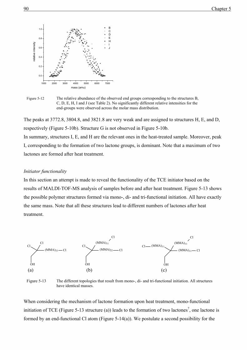
90 Chapter 5
The peaks at 3772.8, 3804.8, and 3821.8 are very weak and are assigned to structures H, E, and D,
respectively (Figure 5-10b). Structure G is not observed in Figure 5-10b.
In summary, structures I, E, and H are the relevant ones in the heat-treated sample. Moreover, peak
I, corresponding to the formation of two lactone groups, is dominant. Note that a maximum of two
lactones are formed after heat treatment.
Initiator functionality
In this section an attempt is made to reveal the functionality of the TCE initiator based on the
results of MALDI-TOF-MS analysis of samples before and after heat treatment. Figure 5-13 shows
the possible polymer structures formed via mono-, di- and tri-functional initiation. All have exactly
the same mass. Note that all these structures lead to different numbers of lactones after heat
treatment.
When considering the mechanism of lactone formation upon heat treatment, mono-functional
initiation of TCE (Figure 5-13 structure (a)) leads to the formation of two lactones7, one lactone is
formed by an end-functional Cl atom (Figure 5-14(a)). We postulate a second possibility for the
1000 2000 3000 4000 5000 6000 7000
0.0
0.2
0.4
0.6
0.8
1.0 B C D E H I J
rela
tive
inte
nsity
mass (amu)
Figure 5-12 The relative abundance of the observed end groups corresponding to the structures B,
C, D, E, H, I and J (see Table 2). No significantly different relative intensities for the end-groups were observed across the molar mass distribution.
OH
ClCl
(MMA)33 Cl
OH
Cl(MMA)11
(MMA)22 Cl
Cl
OH
(MMA)11(MMA)11
(MMA)11 ClCl
Cl
(a) (b) (c) Figure 5-13 The different topologies that result from mono-, di- and tri-functional initiation. All structures
have identical masses.

MALDI of homopolymers 91
lactone formation by one Cl atom of the initiator (Figure 5-14(b)), which is basically the same
reaction as the former lactone formation, i.e. reaction of the ε-OCH3 with the terminal Cl atom.
Table 14 Maximum number of lactones formed in relation to the initiator functionality.
Functionality of initiator Max. nr. of lactones formed Nr. of lactones observed
mono-functional 2 2
di-functional 3 2
tri-functional 3 2
Such dual lactone formation is not possible for initiators with one chlorine atom, such as pTsCl.
Similarly, structures (b) and (c) in Figure 5-13 would show a maximum of three lactones after heat
treatment. In case of a di-functional initiator (Figure 5-13) one of the Cl atoms in Figure 5-14b is
replaced by a bulky polymer chain and the lactone formation needs to take place in the middle of
the polymer chain. However in the “conventional” lactone formation (Figure 5-14b) the two groups
next to the Cl atom (methylester and methyl group) do not hinder the lactone formation, since the
second methylester in the backbone forms the lactone. Although the kinetics of the second
postulated lactone formation will be different, the steric hindrance of the bulky polymer chain is
unlikely to prevent the lactone formation.
The numbers of lactones observed (Table 14) provide strong evidence for a mono-functional
initiation of TCE in ATRP.
Conclusion
MALDI-TOF-MS is demonstrated to be a very powerful technique for end-group analysis to study
initiator functionalities, as long as well-resolved spectra can be obtained.
The MALDI-TOF-MS analysis of PMMA-pTsCl confirms the formation of lactones upon thermal
treatment. Furthermore, the heat treatment increases the resolution of MALDI-TOF-MS spectra and
C O
CCH2
C
CH3 CH3
O
CH2OCH3
O
CCH2CCH2
O
OCH3
CH3
O
OCH3
CH3
OH
ClCl
n-1
CH3Cl
n-1CH2CCH2
CH3
O
OCH3
C CH2 C CH2 C Cl
O O O
OCH3OCH3OCH3
CH3 CH3 CH3
OH
ClCl
(a)
C O
CCH2
C
CH3 CH3
O
CH2OCH3
O
CCH2CCH2
O
OCH3
CH3
O
OCH3
CH3
OH
ClCl
n-1CH3Cl
O C
CCH2
C
C O
CCH2
C
CH3 CH3
O
CH2OCH3
O
CCH2
O
OCH3
CH3CH3
O
Cl
OH
n-1
(b) Figure 5-14 (a) Schematic illustration of the reaction by which an end-functional chlorine atom leads to lactone
formation. (b) Schematic illustration of the reaction by which a chlorine atom at the initiator leads to lactone formation.

92 Chapter 5
simplifies the end-group characterization of polymer systems with weak carbon-halogen bonds. The
results of the MALDI-TOF-MS analysis of PMMA-TCE samples before and after thermal
treatment, in combination with the maximum number of lactones formed, prove the mono-
functional initiation of TCE.
5.3.2 The use of the ECF function
The crucial part in the work described above is the correct interpretation of spectra obtained by
MALDI. In this section the strength of the ECF function is shown.
The ECF of the earlier discussed spectra (Figure 5-10) is shown in Figure 5-15.
The ECF function not only calculates the masses of all end groups present in the spectrum, but also
improves the resolution of the computed end groups. The improved resolution helps to assign and to
exclude possible structures. The labels A through J corresponds to the structures in Table 13. The
subscript of each label refers to the most abundant theoretical-isotope end-group mass of the
corresponding structure and, if present, should be found at the “top” of an isotope pattern (as long
as no isotope overlap takes place). Structure B has an end-group mass of 112.94 amu and is clearly
not on the “top” of the isotope pattern compared to structure I. To exclude peak overlap, the isotope
pattern should be considered as discussed in the previous section. Since their most abundant isotope
0 49.6 99.2 148.8 198.4 248.0
ECF
162.0061.96
128.0227.98 229.06
198.0480.00 180.0398.01145.9945.96
25.99 126.03
After heating
112.0111.97 212.05
49.35 149.40150.4050.35
166.6466.59116.5416.49 216.59
200.44100.39233.4733.37 133.42
182.4982.44
Before heating
B112.94
C98.90
A149.40
D76.48
E62.46
F48.43
G40.02H25.99
I11.97
J98.06A149.40
Figure 5-15 End-group correlation function (ECF) of spectra shown in Figure 5-10. The labels A through J
correspond to the structures in Table 2. The label subscript refers to the most-abundant theoretical-isotope end-group mass of the corresponding structure.
27.9825.99
H25.99
61.96
E62.46
43

MALDI of homopolymers 93
is not located on the “top” of an isotope pattern, peaks A, D, G and F are either absent, or show
isotope overlap. The latter suggests the amount of these structures to be negligible. Structures C and
J may show isotope overlap, whereas the remaining structures E and H can be easily assigned.
However, the ECF function reveals some new insights in the two structures H and E and this will be
discussed in more detail.
The ECF “isotope distribution” represents an average isotope distribution of the peaks within a
chosen mass range and it does not correspond to the isotope distribution of the end-group structures.
The structures H and E are obviously too broad to contain zero or one Cl atom, respectively (see
Table 13). The insert of Figure 5-15 reveals that structure H seems to be “bimodal” and structure E
could be the result of two overlapping distributions, both with a mass difference of only two amu.
The PMMA-pTsCl system indicated the loss of a Cl atom by, besides lactone formation, a cleavage
of an HCl group (formation of a double bond, see Figure 5-9). No evidence was found for other end
groups such as a saturated bond9(the exchange of a Cl atom for a H atom).
For PMMA-TCE, structure H will be observed after one lactone formation and twice the loss of the
(remaining) Cl atoms. In case of Figure 5-13b, each Cl atom has at least one H atom available for
HCl cleavage resulting in double bonds. However, the loss of two HCl groups and the formation of
a lactone in case of Figure 5-13a or Figure 5-14a is impossible, due to the formation of two double
bonds on one and the same carbon atom. The only way to split off two HCl groups is via hydrogen
abstraction of other species, resulting in one double bond (see Figure 5-16) or via the loss of Cl2 and
the rearrangement of one hydrogen atom.
The suggested structure has an end-group mass that is of two amu higher than structure H. But, if
the lactone formation takes place at the initiator side (Figure 5-14b) than the remaining two Cl
atoms at the initiator and the “active” side can easily undergo HCl cleavage which corresponds with
the structure H. The broad isotope distribution of structure E may be the result of two overlapping
isotope distributions, also with a mass difference of two amu.
The structure of Figure 5-13b (bi-functional initiation) cannot lead to structures as shown in Figure
5-16 due to the fact that there are always hydrogen atoms present for the HCl cleavage and no
n-1
CH3
O
CH3
O OO
CH3
CH3
O
O
CH3HO
Cl
Cl
n-1
CH3
O
CH3
O OO
CH3
CH3
O
O
CH3HO
Figure 5-16 The loss of two Cl atoms after lactone formation cannot lead to more than one double bond, as long as the lactone is located at the end of the chain.

94 Chapter 5
evidence was found for the exchange of a Cl atom for a H atom (which could theoretically lead to
the same structure as shown in Figure 5-16) in the case of PMMA-pTsCl.
In the case where TCE is mono-functionally initiating and the lactone formation occurs at the
“active” end of the chain, the loss of two Cl atoms must lead to structures with two amu difference
compared to the loss of the HCl molecules. The absence of these structures in PMMA-pTsCl
systems excludes the di-functional or tri-functional initiation of TCE since a structure with two amu
difference, compared to structure H, cannot be formed. In addition to the previous conclusion, the
number of lactones formed and the use of the ECF function both support the mono-functional
initiation of TCE.
In summary, the ECF improves the resolution of a spectrum since it takes the entire mass range into
account. The improved resolution lead to a more-accurate interpretation of spectra and, it can reveal
small changes in isotope patterns, which are hard to observe from an enlarged part of a spectrum.
One may call the ECF the “end-group fingerprint”, since it includes all the end-group information
present in the spectrum for homopolymers. The end group analysis for copolymers will be
discussed in the next chapter.
In some cases the ECF function is not accurate enough to distinguish between end-group masses.
An accurate end-group-resolution function may help, as shown in the next sections.
5.4 Copolymerization of polyketones
Over the last decades numerous new well-defined transition-metal-based polymerization catalysts
have been reported. The so-called “single-site” catalysts may not always behave as such, since
polydispersities in excess of two have been observed. Polymers which are formed via “single-site”
catalysts are supposed to yield a Flory-Schulz molar-mass distribution with a polydispersity of two.
The Flory-Schulz distribution is based on the assumption that polyaddition of monomers at
equilibrium conditions is independent of the size of the molecule. The high polydispersities found
in practice have been attributed to the occurrence of “multiple-site” catalyst during the
polymerization.
The copolymerization of ethylene and carbon monoxide is known to lead to perfectly alternating
polyketone. The proposed mechanism of the copolymerization is described elsewhere1.
In this study the end groups of the perfectly alternating copolymerization were studied by MALDI-
TOF-MS. The MMDs obtained with MALDI and SEC was compared to the theoretical Flory-
Schulz distribution.

MALDI of homopolymers 95
Materials
Phosphorus trichloride (PCl3,Aldrich, 99.999%), diethylamine ((Et2)2NH ,Aldrich, 99.5%), diethyl
ether ((Et2)2O were distilled before use. N,N,N′,N′- tetramethylethylenediamine (TMEDA, Aldrich
99%) was refluxed over CaH2 and distilled before use. Acrylonitrile (Aldrich, 99%) was degassed
before use. Reacting gases, carbon monoxide (CO) and ethylene were supplied by Hoek Loos (CO:
99.97% pure, ethylene: 99.95% pure). Pd(acetylacetonate)2 (i.e. Pd(acac)2 was supplied by
Degussa. hydrochloric acid diethyl ether solution (HCl/Et2O, Aldrich, 2M), Aldrich, 98.0%),
butyllithium solution, 2.5 M in hexane(n-BuLi), lithium aluminum hydride (LiAlH4, Aldrich,
reagent grade 95%), potassium hydroxide, (KOH, VWR) and 1,1,1,3,3,3-Hexafluoro-2-propanol
(HFIP, Biosolve, Valkenswaard, the Nederlands), di- p-Tolylether (Aldrich, 99%) and
Trifluoromethanesulfonic acid (CF3SO3H, Aldrich, 99%) were used as supplied.
Synthesis of the palladium(II) complex
Starting from di-p-tolylether, the synthesis of the diphosphine ligand has been accomplished
according to the scheme shown below, following a procedure similar to the one reported in
literature.10
The palladium complex suitable for the catalysis was prepared stepwise starting from Pd(acac)2 (see
scheme below) following the literature procedure.11
Experimental
In a typical experiment of copolymerization of ethylene and carbon monoxide, a solution of the
desired palladium complex (0.02 mmol) in 10 ml of anhydrous MeOH was injected, under argon
atmosphere, into a 75 mL stainless-steel autoclave, previously evacuated by a vacuum pump. The
OO
PCl2PCl2
n BuLiTMEDA
iii. HCl/Et2Oii. ClP(NEt2)2
i.
Figure 5-17 The synthesis of the PP-ligand.
PPO
R R R R
LiAlH4
CN
THF
KOH
iv.
v.
R= CN
2
Pd(CH3CN)4( CF3SO3)2
CH3CNPd
O
P P RR
RR
CH3CN NCCH3
2 CF3SO3
PP
O
R R R R
Figure 5-18 The synthesis of the palladium(II) complex.
2Pd(acac)2
CF3SO3HCH3CN
Pd(NCCH3)4(PP)2+
i)
ii) PP ligand
[ ] [ CF3SO3 ]

96 Chapter 5
autoclave was flushed three times with 3 bar of ethylene, then pressurized with ethylene at 25 bar
and carbon monoxide at 25 bar at room temperature and then heated to 60ºC. Stirring (1000 rpm)
was applied during the reaction. After 2 hours, the reaction was stopped by cooling the autoclave
using an ice bath. After the unreacted gases were released, the reaction mixture was filtered. The
white solid was washed with methanol and dried under reduced pressure. MALDI was performed
on the solid fraction.
Size-Exclusion Chromatography (SEC)
SEC analyses were performed on a system, which consisted of a two-column set (PSS PFG
columns linear XL, Polymer Standards Service), an isocratic pump (Gyncotek P580, Separations,
flow rate of 0.4 mL/min), an ultraviolet (UV) detector (Waters 486, 230nm) and a differential
refractive-index (DRI) detector (Waters 410) as concentration detectors, and HFIP as eluent.
MALDI-TOF-MS instrument
The instrument conditions, matrix and salt concentration used are the same as described in section
5.3.1. The sample was dissolved in HFIP. The best spectra were obtained after first depositing the
sample on the target (0.2µL) and subsequently adding the mixture of the matrix and salt solution.
5.4.1 Results and discussion
A typical spectrum of the ethylene-carbon-monoxide copolymer is shown in Figure 5-19. It is the
perfect alternating behavior of the copolymer which makes the spectrum look like that of an
ordinary homopolymer with a “total” repeat mass of a CO unit and an ethylene unit11,12. The insert
(upper right corner of Figure 5-19) suggests the presence of at least two different end groups.
However, the mass difference between the peaks at 1583.736 amu and 1611.732 amu corresponds
to either the mass of a CO unit (28.0104 amu) or an ethylene unit (28.0432 amu). With the use of
the mathematical tools described in section 5.2 we tackle the first question: What are the exact end-
group masses?

MALDI of homopolymers 97
For completeness, the autocorrelation function (ACF) returns the combined mass of the repeat units
of CO and ethylene, 56.048 amu. The outcome of the ACF always returns a slightly lower value
than the theoretical mass of a CO-Ethylene unit (56.064 amu), as explained in section 5.2.3.
Figure 5-21 shows the end-group-correlation function of the copolymer. The two dominant peaks in
the spectrum suggest end-groups masses of 31.999 amu and 3.934 amu. Note that all end-group
masses higher by the repeat mass unit (56) are part of the general solution given by equation (5.4).
It is surprising that the mass difference of the two end-group masses coincides with the mass of
exactly one repeat unit of either a CO or an ethylene unit. A more-plausible explanation would be
termination of the growing polymer after only one CO or ethylene has been incorporated instead of
a CO-ethylene unit. Also relatively small defects in the copolymerization (and not being perfectly
alternating) lead to a different end group. In literature the mechanism of CO/Ethylene
copolymerization has been proposed by Drent and coworkers1. It is shown in Figure 5-22.
0 15 30 45 60 75
AC
F
56.048
1.00157.049
1.997 58.04654.051
2.997 59.04653.05128.016
3.998 60.047
0 15 30 45 60 75
AC
F
56.048
1.00157.049
1.997 58.04654.051
2.997 59.04653.05128.016
3.998 60.047
Figure 5-20 The autocorrelation function of the spectrum shown in Figure 5-19.
Mass (amu)
1017 1734 2451 3168 38850
50
100
Inte
nsity
(%) 1583.736 1639.764
1695.792
1611.732 1667.752
Mass (m/z)1017 1734 2451 3168 3885
0
50
100
Inte
nsity
(%) 1583.736 1639.764
1695.792
1611.732 1667.752
Mass (m/z) Figure 5-19 A spectrum of an ethylene-carbon-monoxide copolymer. The perfectly alternating copolymer
makes the spectrum look like a homopolymer. All species are charged with potassium. The insert suggest the presence of at least two different end groups.

98 Chapter 5
The following structures were suggested to arise from after termination by protonolysis or
methanolysis: di-ketones, keto-esters and di-esters. At low temperatures (< 85oC), the majority of
the products are keto-esters and keto-ethers, with only a small quantity of di-esters and diketones.
At higher temperatures the ratio di-ketones/keto-esters/di-esters gets close to 1:2:11. Since the
experiments were performed at low temperatures, the majority of the expected products are keto-
esters.
The general forms of the end-group masses are listed on the top right of Figure 5-22.
nCH2CH2C
O
OCH3H3COC
O
nCCH2CH2
O
HHCH2CH2
nCCH2CH2
O
HCH2CH2Pd
Di-ketone
Di-ester
Keto-ester n
CH2CH2C
O
OCH3H
n
CCH2CH2 HH3CO
O
C2H4
CH3OH
C2H4
CH3OH
CO
CO nCH2CH2C
O
OCH3CPd
O
CH3OH
Pd O C H 3
Pd COCH3
O
nCH2CH2C
O
OCH3Pd
COC2H4
n n-1
COC2H4
n-1 n
Pd H
Pd C H 2C H 2H
nCCH2CH2
O
HPdIn
In P
P
P
H
H M
M P
(A) (B)
In=Initiation P=Propagation H=Protonolysis M=Methanolysis
Di-ketone = ( ) nmm EtCO ⋅++046.30
Keto-ester = ( ) nmm EtCO ⋅++026.32
Di-ester = ( ) COEtCO mnmm +⋅++036.62
Figure 5-22 Proposed mechanism of carbon monoxide and ethylene copolymerization1.
CH3OH
Keto-ester
0 15 30 45 60Mass (amu)
ECF
31.999
32.995
33.989
34.986
60.0043.93435.984 61.0024.932
55.985 61.9995.929
0 15 30 45 60Mass (amu)
ECF
31.999
32.995
33.989
34.986
60.0043.93435.984 61.0024.932
55.985 61.9995.929
Figure 5-21 The end-group-correlation function of the spectrum shown in Figure 5-19.

MALDI of homopolymers 99
The calculated end-group-mass of 31.999 amu corresponds with the suggested structure of the keto-
ester. However the other end-group-mass, 3.934 amu, cannot be explained by one of the suggested
structures above. The mass difference of the end groups (28.065 amu) +0.05/-0.95 amu (see section
5.2.2) is either a CO unit or an ethylene unit (the error is too large to assign the mass difference to
either). The mechanism in Figure 5-22 suggests in each initiation-propagation-termination cycle (A
and B) always a prefectly alternating structure. A double ethylene insertion is known to be possible,
whereas a double CO insertion does not occur for thermodynamic reasons13,14.
With the HRECF (see section 5.2.2) the mass difference of the end groups could be assigned to the
mass of a CO unit.
There are only two possibilities to add a CO unit to the keto-ester. The first possibility is
straightforward. Add either a CO unit or subtract one ethylene unit (minus one ethylene unit plus
the mass of the repeat unit, or the addition of a CO unit results in the same mass). The end group
becomes an aldehyde. The second possibility is subtracting an ethylene unit. Here, we assume that
at least once the double-ethylene insertion took place. Two methods were employed to find defects
in the alternating system. The first test simply calculates the mass difference as a function of the
number of repeat units. In case a defect (one double-ethylene insertion) is present, the mass
difference will be 0.037 amu higher.
Figure 5-24 shows the persistent mass difference of consecutive repeat units as function of the
number of repeat units. Due to a loss of resolution with increasing number of repeat units, the mass
difference starts to scatter. The linear fit indicates an average constant mass difference and,
therefore, no evidence of one (or more) double ethylene insertions was found. The second method
implies the use of an internal calibration standard. An internal calibration standard eliminates the
error of spot-to-spot variation, which is at least 0.02 amu and thus not acceptable in the present
case. In this procedure a polymer with known end groups was added to the sample and spotted on
the target. The error in the internal calibration standard was found to be less than 0.003, amu which
was sufficient. An enlarged part of the spectrum can be seen in Figure 5-25. The excellent match
between the perfectly alternating keto-ester structures again proves the error-free alternating
system.
27.97805 28.01027 28.04248
28.03127.994
27.97805 28.01027 28.04248
28.03127.994
EC
F HR
EC
F HR
Figure 5-23 The solid Gaussian peak at 27.994 corresponds to the mass of CO whereas 28.031 corresponds to the mass of ethylene. The experimental values with an average of 27.978 ±0.02 amu indicate the CO mass difference of the end groups.

100 Chapter 5
The perfectly alternating copolymerization leads to the conclusion that the mystery peak can only
be explained by an aldehyde end group. No further attempts were made to assign the remaining end
groups due to the weak intensity as shown in Figure 5-19.
1415.0746 1416.2922 1417.5098 1418.7274 1419.9450
1415.5821 1416.58551417.5873
1415.6549 1416.65831417.6601
1415.6185 1416.62191417.6237
1415.61531416.6203 1417.6117
24
CH2CH2C
O
OCH3H
K+
23
CH2CH2C
O
OCH3CH2CH2H
K+
2
23CH2CH2C
O
OCH3CH
O K+
2
Figure 5-25 The upper trace is the measured sample after internal calibration was applied. The lower traces are the simulated spectra of the given structures on the right side of the picture. Although the bottom-trace structure is not thought to occur, it is depicted here for completeness.
Mass (amu)
20 30 40 50 60 70 8055.4
55.6
55.8
56.0
56.2
56.4
number of repeat units Figure 5-24 Mass difference of consecutive repeat units as a function of the number of repeat units. The
upper solid line indicates the expected mass deviation (0.037 amu) if double-ethylene insertion would take place once. The bottom solid line indicates the opposite mass deviation (-0.037 amu). The dashed line presents the linear fit.

MALDI of homopolymers 101
The molar mass distribution (MMD)
In order to compare the molar-mass distribution to the theoretical Flory-Schulz distribution, some
modifications need to be made. The equation describing a Flory-Schulz distribution is given below.
( )2 11 iiw i p p −= − (5.9)
Where iw is the weight fraction, i the chain length, and p the degree of polymerization. For a
copolymer, the chain length is not exactly proportional to the molar mass, since monomers can have
different masses. However, in this case the mass difference of the monomers can be safely
neglected with respect to the resolution of SEC.
As described in section 4.3.1 equation 4-3, the number distribution is proportional to the
logarithmic MMD by M2. Since i iw n M= , the weight distribution is thus proportional to the MMD
by M. The chain length can be related to the molar mass, resulting in the modified Flory-Schulz
distribution.
( )12(log ) 1 ln(10)A B
Mm m
A B
Mw M p p Mm m
−+
⎛ ⎞= −⎜ ⎟⎜ ⎟+⎝ ⎠
(5.10)
Where Am and Bm are the masses of the monomers ( A Bm m≈ ). Note that the entire MMD is
described by only one parameter, p.
Figure 5-26 shows the MMD obtained by SEC and by MALDI. The MMD is somewhat narrower
than the theoretical Flory-Schulz distribution. No explanation could be given for the shape of the
obtained MMD. Due to the low UV absorption of polyketones at 230 nm, no useful UV signal was
obtained. Despite the shape of the MMD, the polydispersity did not exceed the value of two. The
synthesized palladium(II) complex (see Figure 5-18) acts like a single-site catalyst.
5.5 Conclusions
The most abundant end groups in the MALDI-TOF-MS spectrum were assigned to a keto-ester and
to an aldehyde. No other structures, such as, di-keto-ester or di-ketone were observed. The
copolymerization of CO and ethylene results in a perfectly alternating copolymer. No evidence of
double ethylene insertion was observed. The MMD obtained by SEC and MALDI was found to be
in good agreement with, but somewhat narrower than the Flory-Schulz distribution. No explanation
could yet be given for the obtained shape of the MMD.

102 Chapter 5
In summary, the end-group correlation function (can be used to determine end-group-masses within
0.02 amu. A typical example is the difference between a CH4 group and a O atom. In contrast to the
ECF function, some brute processing power is needed to obtain an with a resolution of 0.001 amu,
which makes this function less attractive for daily-routine data-analysis.
The ECFfunction can also be used to study the presence of small defects in the polymer sequence of
monomers of nearly the same mass.
However, the majority of the copolymer systems contain monomers of different masses and
different topologies, i.e. random, gradient, etc. The data analysis of such complex copolymers is
discussed in the next chapter.
1.5 2.0 2.5 3.0 3.5 4.0
0.0
0.2
0.4
0.6
0.8
1.0 Flory-Schulz SEC MALDI
Rel
ativ
e in
tens
ity
LogM Figure 5-26 A SEC chromatogram of a polyketone. The MALDI trace seems to fit very well to the
high-molar-mass tail of the distribution. The MMD is somewhat narrower than the theoretical Flory-Schulz distribution.

MALDI of homopolymers 103
Reference List 1. a) Drent, E.; Budzelaar, P. H. M. Chem. Rev. 1996, 96 (2), 663-681; b) A. Sen, Catalytic
Synthesis of Alkene-Carbon Monoxide Copolymers and Cooligomers, Catalysis by Metal Complexes, Volume 27. Kluwer AP, Dordrecht, 2003, 16, 1; c) P.W.N.M. van Leeuwen, Homogeneous Catalysis, Kluwer AP, Dordrecht, 2004, 12, 239; d) Drent, E.; Budzelaar, P. H. M. Chem. Rev. 1996, 96 (2), 663-681; e) C. Bianchini, A. Meli, W. Oberhauser, Dalton Trans., 2003, 2627.
2. Wallace, W. E.; Guttman, C. M.; Antonucci, J. M. American Society for Mass Spectrometry 1999, (10), 224-230.
3. Hawker, C. J.; Bosman, A. W.; Harth, E. Chem. Rev. 2001, 101, 3661-3688.
4. George, M. K.; Veregin, R. P. N.; Kazmaier, P. M.; Hamer, G. K. Trends in Polymer Science 1994, 2, 66-72.
5. Destarac, M.; Matyjaszewski, K.; Boutevin, B. Macromol. Chem. Phys. 2000, 201, 265-272.
6. Haddleton, D. M.; Jasieczeck, C. B.; Hannon, J. M.; Shooter, A. J. Macromolecules 1997, 30, 2190-2193.
7. Borman, C. D.; Jackson, A. T.; Bunn, A.; Cutter, A. L.; Irvine, D. J. Polymer 2000, 41 (15), 6015-6020.
8. Haddleton, D. M.; Shooter, A. J.; Heming, A. M.; Crossman, M. C.; Duncalf, D. J.; Morsley, S. R. In "Controlled Radical Polymerization"; Matyjaszewski, K. , Ed. ; ACS Symposium Series No. 685; AmericanChemical Society: Washington DC, 1997, 284.
9. Singha, N. K.; Rimmer, S.; Klumperman, L. European Polymer Journal 2004, 40 (1), 159-163.
10. a) Dibowsky, H.; Schmidtchen, F. P. Tetrahedron 1995, 51, 2325-2330; b) M.T. Reetz, D. Moulin, A.Gosberg, Organic Letters, 2001, 3(25), 4083; c) R.T. Boere', J.D. Masuda, Can.J.Chem., 2002, 80, 1607; d) H.Dibowsky, F.P. Schmidtchen, Tetrahedron,1995,51(8), 2325-2330,; e) M Caporali,.; Müller, C.; Staal, B.B.P.; Tooke, D. M.; Spek, A. L.; van Leeuwen, P. W. N. M., manuscript in preparation.
11. a) Drent, E.; Van Broekhoven, J. A. M.; Doyle, M. J. J. Organomet. Chem. 1991, 417, 235-251; b)Wendt, N-F.K. Kaiser, L.I. Elding, J.Chem.Soc.,Dalton Trans., 1997, 4733-4737; c) K.Li, P.N. Horton, M.B. Hursthouse, K.K. Hii, J.Organomet.Chem., 2003, 665, 250.
12. Drent, E. Chem. Abstr. 1985, 102, 46423.
13. Chen, J.-T.; Sen, A. J. Am. Chem. Soc. 1984, 106, 1506.
14. Sen, A.; Chen, J.-T.; Vetter, W. M.; Whittle, R. R. J. Am. Chem. Soc. 1987, 109, 148.

104 Chapter 5
Appendix 5A Some of the possible structures regarding Table 13 are depicted below.
Structure A:
K+
m
n
p
O
OCH3
ClCH3
O
HO
ClO
OCH3
O
CH3
CH3
ClCH3
CH3
K+
nCH3
Cl
ClCH3
O
HOCl
O
CH3
K+
n
p
O
OCH3
ClCH3
O
HOCl
O
CH3ClCH3
CH3
Structure B:
K+n
ClCH3
O
HO
Cl O
CH3K+
n-1
CH3
O
HO
Cl O
CH3
CH3
O
O
CH3
Cl
Structure C:
K+n-1
CH3
O
OO
CH3
CH3
O
O
CH3HO
Cl O
CH3
Cl
K+n-1
ClCH3
O
O
CH3
OO
CH3
OH
Cl
Structure D:
K+
m- 1
n-1
CH3
O
HO
Cl
CH3 OCH3
O
O
OCH3
O
CH3
CH3
O
O
CH3
K+n-1
CH3
O
HO
Cl O
CH3
CH3
O
O
CH3
Structure E:
K+n-1
CH3
O
OO
CH3
CH3
O
O
CH3HO
Cl O
CH3K+
n-1
CH3
O
O
CH3
OO
CH3
OH
Cl CH3
O
O
CH3
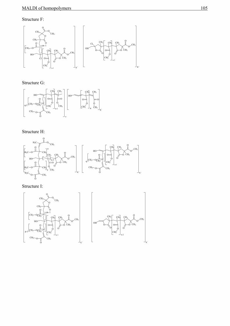
MALDI of homopolymers 105
Structure F:
K+
m- 1
n-1
CH3
O
OO
CH3
CH3
O
O
CH3HO
Cl
O
OCH3
O
OCH3
CH3
O
OCH3
O
CH3 K+
n-2
CH3
O
OO
CH3
CH3
O
O
CH3
O
CH3
OO
CH3
OH
Cl
Structure G:
nK+
CH3
O
CH3
O
CH3
OHO
O
CH3
K+
n-1
q-1
O
OCH3
CH3
O
HOO
CH3
CH3O
O
CH3
CH3
CH3
O
O
CH3
Structure H:
K+
n-1
p
m
CH3
O
O OO
CH3
CH3
O
O
CH3HO
O
OH3C
O
OH3C
CH3
CH3CH3
CH3OH3C
O
H3C OCH3
O
K+
n-1
q
O
OCH3
CH3
O
OO
CH3
CH3
O
O
CH3HO
O
CH3
CH3O
O
CH3
CH3
Structure I:
K+
m- 1
n-1
p-1
O
OCH3
CH3
O
OO
CH3
CH3
O
O
CH3HO
O
OCH3
O
OCH3
CH3
O
OCH3
O
CH3
CH3
CH3O
O
CH3
CH3
K+
n-2
CH3
O
OO
CH3
CH3
O
O
CH3
O
CH3
OO
CH3
OH

106 Chapter 5
Structure J:
O
OCH3
O
OCH3
CH3
O
OCH3
O
OH3C
H3C
K+
n-1
p-1
m-1
CH3
O
O OO
CH3
CH3
O
O
CH3HO
O
OCH3
O
OCH3
CH3
CH3CH3
Outlook and development 107
Chapter 6
6 MALDI of copolymers
6.1 Introduction In the previous chapter it has been shown that, with a precise interpretation of the spectra, MALDI
can reveal information about the molar-mass distribution (MMD) and the end-group masses of
homopolymers. In this chapter the characterization of copolymers will be discussed. Although their
spectra are more complex, with the correct interpretation not only the MMD and the end-group
masses, but even the chemical composition, the topology (random, block or gradient), the block-
length distributions, and the chain-length distributions of copolymers can be measured with
MALDI-TOF-MS. Unfortunately, this information cannot be obtained as the direct outcome of the
analysis. Hence, mathematical operations are needed. Based on the ideas described in this chapter
we developed a program, to visualize the results of the calculations. With this program, within the
limitations of mass spectrometry and the conditions of the developed methods, it is even possible to
analyze copolymer samples for which no information about topology, end-group masses and type of
monomers is available.
6.2 Copolymer analysis
The observed mass of a singly charged copolymer chain in MALDI-TOF-MS can be described by
the following equation:
21 endendionBBAAobs mmmnrmnrmm +++⋅+⋅= (6.1)

108 Chapter 6
Where obsm is the observed mass from a peak in the MALDI-TOF-MS spectrum, Am , Bm , ionm ,
1endm , and 2endm are the masses of the repeat units A and B, the adduct, and the end groups,
respectively. Anr and Bnr are the respective numbers of repeat units A and B.
The autocorrelation function (ACF) as discussed in section 5.2.3, can be applied to spectra of
copolymers as well. The ACF helps to determine the possible types of monomers, which constitute
the copolymer. The complexity of the copolymer obviously influences the accuracy of this method.
In cases where the identification of the monomers is of great interest, other methods, such as,
pyrolysis-gas chromatography mass-spectrometry are probably more reliable.
6.2.1 Copolymer topologies
Copolymers can be classified as random, block, gradient, grafted, or branched copolymers. These
topologies cannot be identified based on only the mass of one polymeric chain, as obtained from a
MALDI-TOF-MS spectrum. For example, the copolymers (random, block, alternating and gradient)
shown in Figure 6-1, have the same molar mass, i.e. the same numbers of repeat units A and B, but
the sequence differs completely. Fortunately, the relative abundance of the peaks in a spectrum is
different for each topology. Therefore, by taking the pattern of all peaks within the entire molar-
mass distribution into account, it is possible to distinguish between e.g. a gradient and a block
copolymer.
= end groups = repeat units
Random Block Alternating Gradient
Figure 6-1 Different types of polymer topologies. The systems above the dashed line are discussed in this thesis.
} End-group distributions Graft
Branched
}
Homopolymers Copolymers
End-group distributions Graft
Branched

Outlook and development 109
The possible combinations to construct a copolymer out of different monomers are numerous. Only
a few are depicted in Figure 6-1 and, hence, classification is needed. First of all, a distinction is
made between homopolymers and copolymers. Secondly, a distinction is made between end-groups
and chain structure, i.e. in what way the number of the different monomer units are incorporated in
the polymer chain.
For a homopolymer, apart from the molar mass distribution, only end-group distributions can be
observed. The only mass differences for different homopolymer topologies are the total end-group
masses. Therefore, no distinction can be made between different topologies, except for grafted
systems, where each molecule contains a different number of (the same) end groups.
For copolymers, the shape of a MALDI spectrum depends on the relative abundance of all
individual chains, on the chain end-groups, and on the structure of the chains. Information on
topology can be obtained from end-group analysis and from the chain structure. Since the latter
gives the best indication of the possible topology, a method to obtain information on the chain
structure from the copolymer spectrum will be discussed first. In section 6.5 the end-group
determination will be discussed.
6.2.2 Copolymer structure
In a first attempt to reveal the chain structure of a copolymer, the relationship between Anr and Bnr
was investigated. For simplicity we assume the end-group mass to be known. The MALDI
spectrum relates peak intensity )(mI and mass. The mass of each peak can be assigned to a
combination of Anr and Bnr . The peak intensity can therefore be written as a function of Anr and
Bnr , ),()( BA nrnrImI → , taking into account the following criterion:
2mmm calcobs ∆≤− (6.2)
21 endendionBBAAcalc mmmnrmnrmm +++⋅+⋅= (6.3)
Where m∆ is the mass accuracy, typically ≤ 0.5 amu and calcm the calculated mass of the most-
abundant isotope in the isotope distribution corresponding to a specific combination of Anr and
Bnr . The entire mass range of the spectrum can be subjected to the criterion of equation (6.2). In
this way each combination of repeat units Anr and Bnr can be related to the measured intensity of
the spectrum, which is defined as the intensity matrix ),( BA nrnrI .
The intensities of the peaks in the spectrum are subject to peak-shape differences, overlapping
isotopes, and isotope broadening. Before we can compute the intensity matrix, the observed
intensities need to be corrected for these effects.
110 Chapter 6
6.2.3 Peak-shape differences
The maximum peak intensity is sensitive to variations in resolution and in peak shape (i.e. tailing,
ringing, and fronting; see section 2.3.1). In MALDI-TOF-MS it is impossible to have exactly the
same resolution in the high- and low-mass regions within one measurement, due to variations in the
initial velocity (see section 2.1.3). Errors due to peak-shape differences and resolution changes are
minimized by summation across half an amu towards both sides of the peak maximum:
∑+
−
=5.0
5.0)(
m
mm mII (6.4)
Where )(mI is the original peak intensity and mI the intensity corrected for resolution differences.
The value of 0.5 amu has not been chosen arbitrarily but represents half of the mass difference
between two consecutive peaks in a well-resolved isotope pattern. Two well-resolved isotopes
always differ by essentially one amu (the mass of a neutron is 1.00866497 amu).
Throughout the text two commonly used terms are summation and integration. As discussed in
section 2.4, summation is performed in the mass domain, whereas integration is always performed
in the time domain. Both results in the same values.
The reason not to sum the entire isotope patterns is that the isotope patterns of different polymer
species overlap.
6.2.4 Overlapping isotopes
Overlap of isotopes is a typical problem of copolymer systems. Neighboring isotope peaks start to
overlap, because of the great number of possible combinations of repeat-unit masses and their
corresponding isotope distributions. Overlap of isotopes affects the areas of the most-abundant
isotopes and, hence, a correction is needed to obtain the correct intensity matrix. This can be
illustrated by an example of a copolymer of styrene and isoprene (Figure 6-2).

Outlook and development 111
In order to correctly integrate the area of each isotope, the relative contributions of the overlapping
isotopes should be known. Therefore, a secondary criterion is required to find all observed
intensities which belong to the same isotope distribution in the spectrum.
To avoid the need for this secondary criterion, only the most-abundant-isotope peak is corrected for
the contribution of the overlapping peaks. In the end, only the area under this peak is needed for
further calculations.
The black/gray colored areas of peak St19Ip29 in Figure 6-2 show the contribution of overlapping
isotopes. The table in Figure 6-2 shows the unbiased (i.e. without overlap) peak intensity of the
most-abundant isotope for the distributions of St17Ip32 and St19Ip29 and the contribution of the
neighboring isotope distributions to its observed intensity. These contributions of the neighboring
isotope distributions are expressed relative to their most-abundant unbiased isotope. For example,
the observed intensity of the most-abundant isotope of St19Ip29 can be expressed in terms of the
unbiased intensity of the most-abundant isotopes of St19Ip29, St17Ip32 and St21Ip26:
Observed intensity of St19Ip29 = 100% of St19Ip29 + 20.8% of St17Ip32 + 9.3% of St21Ip26
Whether intensity or area is used is arbitrary. Since the correction for peak-shape differences
(section 6.2.3) already provides the area of the most-abundant isotope, we will use the area instead
of the intensity in further calculations. If in the following text, the peak of a given number of repeat
units (e.g. ,A Bnr nrI ) is mentioned, it always refers to the most-abundant peak of the isotope
distribution.
4107 4112 4117 4122 4127 4132 Mass (m/z)
10
20
30
40
50
60
70
80
90
100
% Intensity
4112.1 4116.1
Figure 6-2 The simulated isotopic distribution of four polymer chains containing different numbers of repeat units styrene (St) and isoprene (Ip): end groups: t-butyl and H: charge Ag+. The table shows the contribution of the overlapping peaks, in percentages at peak 4116.1 amu and at 4120.0 amu.
St15Ip35 St17Ip32 St19Ip29 Peak intensity
Overlapping peaks
St17Ip32 St19Ip29
St15Ip35 20.6% 0%
St17Ip32 100% 20.8%
St19Ip29 9.4% 100%
St21Ip26 0% 9.3%
4120.0 4123.9
( )bnranrmnrnr BABAP +− ,,, ( )bnranrmnrnr BABA
P −+ ,,,
( )BABA nrnrmbnranrP ,,, +− ( )BABA nrnrmbnranrP ,,, −+
St21Ip26
( )BABA nrnrmnrnrP ,,,

112 Chapter 6
To correct a peak area, one needs to know the unbiased peak areas of the overlapping distributions.
Those peak areas, on their turn, depend on the unbiased peak areas of their overlapping
distributions, and so on. For practical reasons, we only take two consecutive neighboring isotope
distributions into account. Furthermore, we assume the unbiased peak area of the second
neighboring distribution to be equal to the unbiased peak area of the first neighboring distribution.
We also assume both neighboring isotope distributions to be the same. For example, let Io be the
area without overlap, to correct ( )29,19,29,19 mIo we assume (on the left side of the peak) ( )32,17,32,17 mIo and
( )35,15,35,15 mIo to have the same unbiased area and equal percentages
( ( ) ( )BABABABA nrnrmbnranrbnranrmbnranr PP ,,,,,2,2 +−+−+− = ). The same assumption can be made for the right side of the
peak so that ( )26,21,26,21 mIo equals ( )23,23,23,23 mIo and ( ) ( )BABABABA nrnrmbnranrbnranrmbnranr PP ,,,,,2,2 −+−+−+ = .
The total observed area can be written as the sum of the individual overlapping isotopes.
( ) ( ) ( ) ( ) ( )BABABABABABABABABABABA nrnrmbnranrnrnrmbnranrnrnrmbnranrnrnrmbnranrnrnrmnrnrnrnr PIoPIoIoI ,,,,,,,,,,,,,,,, −+−++−+− ⋅+⋅+=
(6.5)
( ) ( ) ( ) ( ) ( )bnranrmnrnrnrnrmnrnrbnranrmbnranrbnranrmbnranrbnranrmbnranrbnranr BABABABABABABABABABABAPIoPIoIoI +−+−+−+−+−+−+−+− ⋅+⋅+= ,,,,,,,,2,22,2,2,2,,,,
(6.6)
( ) ( ) ( ) ( ) ( )bnranrmnrnrnrnrmnrnrbnranrmbnranrbnranrmanrbnrbnranrmbnranrbnranr BABABABABABABABABABABAPIoPIoIoI −+−+−+−+−+−+−+−+ ⋅+⋅+= ,,,,,,,,2,22,2,2,2,,,,
(6.7)
Where Io is the area without overlap or unbiased area, I the observed area in the spectrum at a
given number of repeat units, and P the percentage relative to the most-abundant peak of the
corresponding isotope distribution. The number of repeat units ( )BA nrnr , indicates the isotopic
distribution, whereas the mass ( )BA nrnrm , indicates the position of the most-abundant isotope peak
used to calculate the percentage P . The percentage P is expressed as the percentage relative to the
most-abundant isotope of the corresponding isotope distribution. The numbers a and b are integers,
corresponding to the nearest neighboring isotopes relative to Anr and Bnr . In order to compute the
percentage P, the theoretical isotope distribution is used1. The outcome of the theoretical isotope
distribution is a discrete set of probabilities corresponding to exact masses with a mass interval
depending on the nature of the isotopes. Each peak mass of the isotope distribution corresponds to
such an exact mass. In the simulation of the isotope pattern, shown in Figure 6-2, instrumental
broadening is taken into account. The broadening can be assumed to be identical for the entire

Outlook and development 113
isotope distribution. Therefore, the areas in Figure 6-2 are directly related to the outcome of the
theoretical isotope distribution. As long as we express the intensities of isotopes relative to the
most-abundant isotope, the outcome of the theoretical isotope calculations is already a percentage
(P).
After writing the Io ’s explicitly the following equation is obtained:
( ) ( ) ( )142421231223111
21211212211 ,,,, PPPPPPPPPPPPPP
IPPPIPPPIPPPPIo bnranrbnranrnrnr
nrnrBABABA
BA ⋅⋅+⋅+⋅⋅+⋅−−⋅+−−⋅+⋅+⋅+⋅+⋅⋅−−−−
= −++−
(6.8)
Where:
( )BABA nrnrmbnranrPP ,,,1 +−= , ( )BABA nrnrmbnranrPP ,,,2 −+= , ( )bnrnranrmnrnr BBABAPP +−= ,,,,3 and
( )bnrnranrmnrnr BBABAPP +−= ,,,,4
Note, that the integration limits of the overlapping peaks (Figure 6-2) are not exactly the same, as
can be seen from the position of the peak maximum (all peaks have exactly the same width, thus a
change of the position of the peak maximum is related to a corresponding change of the integration
limits). The peak ( )BABA nrnrmbnranrP ,,, +− is slightly shifted to the left, whereas ( )BABA nrnrmbnranrP ,,, −+ is
slightly shifted to the right. This shift is due to the exchange of hydrogen atoms with a carbon atom.
The mass difference between one C12 and twelve H1 atoms is smaller then 0.1 amu and, hence, the
error of not taking the same integration limits around the individual isotopes can be neglected. The
result for the corrections can be found in table 15.
Table 15 The isotope distributions of a given number of styrene units and isoprene units were summed according to a theoretical intensity distribution. After the summation, the observed intensities were corrected for the overlap of isotopes. The relative difference of the observed and theoretical intensities is shown.
Peak Theoretical
Intensity Error# (%) Error after
correction (%) PS13IP38 0.0073 1.8 0.3 PS15IP35 0.0184 1.2 1.2 PS17IP32 0.0312 2.0 1.5 PS19IP29 0.0358 0.0 1.6 PS21IP26 0.0276 5.2 0.9 PS23IP23 0.0144 14.3 1.8 PS25IP20 0.0051 27.1 7.8 Summed intensity 0.140 0.144 0.141
# The observed intensity increases due to the overlap of isotopes. The intensity is normalized by peak height, whereas the intensity of the correction method is not normalized.

114 Chapter 6
6.2.5 Isotope broadening
Isotope distributions become broader with increasing mass. The relative contribution of the most-
abundant isotope, with respect to the total area of the isotope distribution, decreases with increasing
mass. Therefore we introduce the isotope-broadening correction factor (IBC). The computation of
the isotope distributions has been based on the work of Yergey1.
∑ ∑ ∑
∑
= =
+=
−==max max max
min0 0,
5.0
5.0,
,
)(
)(
A
A
B
B
BA
abd
abd
BA
BA nr
nr
nr
nr
m
mnrnr
m
mnrnr
nrnr
mp
mpIBC (6.9)
Where
BA nrnrIBC , is the normalized isotope-broadening correction factor, )(, mpBA nrnr is the theoretical
isotope intensity at mass m, abdm is the mass of the most-abundant isotope, and minm and maxm are
the lower and upper limit masses of the isotope distribution )(, mpBA nrnr respectively.
After correcting the intensity for peak-shape differences, overlapping isotopes, and isotope
broadening we plot Anr , Bnr and BA nrnrIc , as a quasi 3D plot2-5 or as a two-dimensional contour
plot6. The latter representation is easier to interpret and is called a “copolymer fingerprint”7.
6.3 Copolymer fingerprints
Copolymer fingerprints are two-dimensional graphical representations of three dimensions (number
of repeat units A, number of repeat units B, and the intensity). These graphical representations, so-
called contour plots, directly reveal information on the polymer architecture, as will be discussed
later.
The methods described in section 6.2.4 correct the observed intensity for isotope overlap and
subsequently compute the intensity matrix. However, the method of isotope overlap requires prior
knowledge on the position of the interfering isotope distributions. Equation (6.8) requires the
integers a and b, i.e. the corresponding position of the nearest neighboring isotopes, to be known.
The next section describes a method to predict these integers. With these predictions, the observed
intensity can be corrected directly. Hence, the intensity matrix can be computed without the need of
any prior knowledge on the position of the nearest neighboring isotopes.
6.3.1 Isotope overlap and isotope interference
Outlook and development 115
In copolymer systems different combinations of repeat units A and B can result in nearly the same
mass. Let us assume a copolymer system where the observed mass ( )obsm can be constructed
( )calcm from only two combinations of repeat units A and B. Both combinations, 11, BA nrnr and
22 , BA nrnr , meet the criterion of mmm calcobs ∆≤− . The given mass interval, m∆ , is determined by
the instrument performance (normally, m∆ <1.0 amu). The observed mass ( )obsm always refers to
the most-abundant isotope. When two (or more) combinations of repeat units meet the criterion
mmm calcobs ∆≤− , isotope interference occurs. Isotope interference can be defined as:
Two (or more) combinations of repeat units with a corresponding most-abundant-isotope-
mass difference smaller than m∆ .
If the difference between the most abundant isotopes does not meet the criterion for isotope
interference, but is within the range of the isotope width, other peaks may overlap with the most
abundant isotope. If in this case the entire width of the isotope distribution is taken into account,
combinations of 11, BA nrnr and 22 , BA nrnr can be found that meet the criterion of Immm calcobs ∆≤− ,
where Im∆ is the width of the isotope pattern. Isotope overlap can be defined as:
Two (or more) combinations of repeat units resulting in isotope distributions where the
most-abundant isotope of one distribution overlaps with a peak from the other distribution.
The mass difference between the most-abundant peaks of the overlapping distributions is
smaller than the width of the isotope pattern ( Im∆ ).
In principle, the problems of isotope interference and isotope overlap are related. Mathematically,
isotope overlap is a simple form of isotope interference. Therefore, isotope overlap will be
discussed first.
To illustrate the problem of isotope overlap we assume a situation as shown in Figure 6-3. We
assume a narrow chemical-composition distribution the sample only consists of two polymer
chains. The width of both isotope distributions equals 11 amu ( Im∆ ) and the mass difference of the
polymer chains ( ( ) ( ), ,A B A A B Bm nr nr m nr nr nr nr− −∆ +∆ ) is 2 amu.

116 Chapter 6
In total six different combinations of repeat units Anr and Bnr can be assigned that meet the
criterion of isotope overlap. This multiple peak assignment leads to overlap of the
contour plots (Figure 6-4). The method developed in section 6.2.4, to correct for overlapping
isotopes, requires the values of Anr∆ and Bnr∆ to be known. The following sections explain the
complicated relation between Anr∆ and Bnr∆ .
6.3.2 Calculation of Anr∆ and Bnr∆ for isotope overlap
The problem of isotope overlap, also known as multiple peak assignment, has been addressed by
Wilczek-Vera et al.3 who proposed the following relationship:
A
B
BB
AA
mm
nrnrnrnr
=−−
21
21
or
A
B
B
A
mm
nrnr
=∆∆
(6.10)
Where Am and Bm are the masses of the repeat units A and B respectively.
A graphical representation of isotope overlap is shown in Figure 6-4. The intensity matrix is
depicted as small black spots on the left side of the figure. If a square around each black spot was
filled with a color indicating its observed intensity, a contour plot is obtained. The solid line in this
figure represents all solutions of Anr and Bnr for a given obsm , whereas the dashed lines represent
the error intervals. The black spots represent the integer combinations of Anr and Bnr . Figure 6-4
shows two data points within the error intervals, i.e. two combinations of Anr , Bnr satisfy the
criterion of Immm calcobs ∆≤− .
Strictly speaking, equation (6.10) is only valid when three out of the four variables
1Anr , 2Anr , 1Bnr , 2Bnr are integers. If integer values are chosen for 1Anr , 1Bnr and 2Anr then the value
Mass (m/z)
10
20
30
40
50
60
70
80
90
100
% Intensity
Figure 6-3 The simulated isotopic distribution of two polymer chains showing isotope interference. In total six different combinations of repeat units Anr and Bnr could be assigned to the peaks of the two polymer chains. This multiple assignment leads to overlap of the contour plots.
Mass difference 11=∆Im amu
),( BBAA nrnrnrnrm ∆+∆−
)2,2( BBAA nrnrnrnrm ∆+∆− )2,2( BBAA nrnrnrnrm ∆−∆+
)3,3( BBAA nrnrnrnrm ∆−∆+
),( BA nrnrm
( 3 , 3 )A A B Bm nr nr nr nr− ∆ + ∆

Outlook and development 117
of 2Bnr cannot be an integer, as long as AB mm is not an exact multiple (which is highly unlikely).
In the following text non integers are marked with a capital N.
Equation (6.10) requires a given Anr∆ and Bnr∆ . However, to minimize the number of input
parameters, it would is attractive if Anr∆ and Bnr∆ can be calculated out of any combination of
repeat units A and B ( ),A Bnr nr . Starting from an arbitrary position in the contour plot of Figure 6-4,
let 1Anr =0 and 1Bnr =0. At a given 2Anr the corresponding 2BNr follows from the equation of the
solid line in Figure 6-4. The masses of both positions are exactly the same:
1 1 2 2A A B B A A B Bnr m nr m nr m Nr m⋅ + ⋅ = ⋅ + ⋅ (6.11)
Taking the starting position into account ( 1Anr =0 and 1Bnr =0) the second index can be left out
( 2A Anr nr= ∆ , 2B BNr Nr= ∆ ) and equation (6.11) can be rewritten as:
A AB
B
nr mNrm
∆ ⋅∆ =
− (6.12)
Equation (6.12) can be used to calculate the value of BNr∆ , but it cannot be used to compute calcm
since calcm , represents the mass of a polymer chain constructed from an integer number of repeat
units. Figure 6-4 illustrates when the nearest integer value of BNr∆ is within the criterion of
Immm calcobs ∆≤− .

118 Chapter 6
The right side of Figure 6-4 shows an enlarged part of the intensity matrix. The big black spot
represents the position of a combination of integer values ( 22 , BA nrnr ). Two other (smaller) black
spots are indicated as ,A Bnr Nr∆ ∆ and 2,A Bnr Nr∆ ∆ representing two non integer values, BNr∆ and
2BNr∆ , for the same Anr∆ . The difference between BNr∆ and 2BNr∆ depends on Im∆ . Im∆
represents the width of the isotopic pattern and is perpendicular to the line representing all solutions
of Anr and Bnr of a given observed mass ( )obsAB mnrnr , . Note that Im∆ is expressed in mass (amu)
whereas the arrow in Figure 6-4 is expressed in terms of Anr and Bnr . Therefore ∆Im is written in
terms of ANr∆ and BNr∆ :
( ) ( )( )
2
2 2,m A B
A B
∆ImI Nr Nr
m m∆ ∆ ∆ =
+ (6.13)
where mI∆ is expressed in terms of ANr∆ and BNr∆ and no longer in mass units. The )cos(ϕ in the
triangle shown in Figure 6-4 leads to the following relation for 2BNr :
ϕ
Anr
Bnr 11, BA nrnr
22 , BA nrnr
⎟⎟⎠
⎞⎜⎜⎝
⎛−
−+++⎟⎟
⎠
⎞⎜⎜⎝
⎛−
⋅=B
obsendendion
B
AAB m
mmmmm
mnrnr 21
BA nrnr ,
Figure 6-4 The solid line presents all possible solutions for Bnr as function of Anr with a constant mass. The dashed lines present the upper and lower limits of a given mass interval. This 2D contour plot visualizes the isotope interference of the combinations of repeat units 1 1,A Bnr nr and 2 2,A Bnr nr . Although the two combinations have a completely different composition, their mass difference is less then m∆ , thus one observed intensity is assigned to two positions of the intensity matrix. Since the ellipse connects all data points with equal intensities, the isotope interference leads to contour overlap as seen at the position of Anr , Bnr . A smaller radius indicates a higher intensity. The dotted lines represent the upper and lower limits of the isotope width interval ( Im∆ ) indicating isotope overlap, i.e. the position of 1 1,A Bnr nr and ,A Bnr nr will show isotope overlap.
22 , BA nrnr
( )B
A
mm
−=ϕtan
,A Bnr Nr∆ ∆
ϕ
( )obsAB mnrnr ,
( )BAm nrnrI ,∆
2,A Bnr Nr∆ ∆

Outlook and development 119
( )( )
( )( )
2
2 2
2 cos tanA B
B BA B
∆Imm m
Nr Nra m m
+∆ = ∆ ±
− (6.14)
Note that the difference between 2BNr∆ and BNr∆ is constant. Substituting equation (6.12) into
(6.14)gives:
( )( )
( )( )
2
2 2
2 cos tanA BA
B AB A B
∆Imm mmNr nr
m a m m
+⎛ ⎞∆ = ∆ ⋅ ±⎜ ⎟ −⎝ ⎠
(6.15)
In Figure 6-4 the position of 22 , BA nrnr is located above ,A Bnr Nr∆ ∆ but it can also be located below
,A Bnr Nr∆ ∆ , indicated by the ± sign in equation (6.15).
The positions of BNr∆ and 2BNr∆ can be calculated as a function of Anr∆ . If an integer exists
within the range ( )2B B BNr Nr Nr∆ ± ∆ −∆ for a given Anr∆ , then the number of repeat units that can
be exchanged equals Anr∆ or, as can be seen in Figure 6-4, AAA nrnrnr ∆=− 21 . To test whether an
integer value is present in the range ( )2B B BNr Nr Nr∆ ± ∆ −∆ the following inequality applies:
( )( )
( )( )
( )( )
( )( )
( )( )
( )( )
1
tancos2
1,tancos
1,tancos
22
2
22
2
22
2
≠
−+
⋅
⎟⎟⎟⎟⎟⎟
⎠
⎞
⎜⎜⎜⎜⎜⎜
⎝
⎛
⎟⎟⎟⎟⎟
⎠
⎞
⎜⎜⎜⎜⎜
⎝
⎛
−+
−⎟⎟⎠
⎞⎜⎜⎝
⎛⋅∆−
⎟⎟⎟⎟⎟⎟
⎠
⎞
⎜⎜⎜⎜⎜⎜
⎝
⎛
⎟⎟⎟⎟⎟
⎠
⎞
⎜⎜⎜⎜⎜
⎝
⎛
−+
+⎟⎟⎠
⎞⎜⎜⎝
⎛⋅∆
BA
BA
BA
BA
B
AA
BA
BA
B
AA
mmamm
∆Im
mmamm
∆Im
mmnrMOD
mmamm
∆Im
mmnrMOD
(6.16)
With AB mm > ,
( )( )
( )( ) B
A
BA
BA
mm
mmamm
∆Im
<−+
<tancos
022
2
, where Anr∆ is a number of integer values of
repeat units A and MOD the modulo. The integer value of Bnr∆ for the given Anr∆ can be
calculated from:

120 Chapter 6
( )( )
( )( )⎟⎟⎟⎟⎟
⎠
⎞
⎜⎜⎜⎜⎜
⎝
⎛
−+
+⎟⎟⎠
⎞⎜⎜⎝
⎛⋅∆=∆
BA
BA
B
AAB mma
mm∆Im
mmnrINTnr
tancos
22
2
(6.17)
Finally, the width of Anr∆ depends on the ratio BA mm and on the width of the isotope pattern
( )∆Im . Under normal MALDI-TOF-MS conditions the accuracy of the acquired spectra is greater
than the mass difference of two consecutive isotopes. Therefore, the isotope overlaps are the result
of the existence of isotope distributions, as long as BA mm is not an exact multiple. In systems
where BA mm is an exact multiple, Anr∆ is solely determined by the ratio BA mm . This is due to
the fact that the exchange of Anr∆ for Bnr∆ with exactly the same mass is not affected by the
accuracy of the measurement and, therefore, equation (6.14) is not valid.
To conclude, Anr∆ can be exchanged for a certain Bnr∆ resulting in nearly the same calcm . Hence,
isotope overlap occurs. At such a value of calcm the measured intensity equals the summed intensity
of the two isotope distributions. With the use of equations (6.17) and (6.16) all solutions for Anr∆
and Bnr∆ can be calculated in order to locate their overlapping masses. After obtaining the
solutions for Anr∆ , the occurrence of isotope overlap can be verified, starting from the most
abundant peak in the entire spectrum. In case no overlap of isotopes is observed, the chemical
composition is either narrow enough to prevent overlap or one of the two combinations Anr , Bnr is
very weak in intensity.
6.3.3 Calculation of Anr∆ and Bnr∆ for isotope interference
To calculate Anr∆ and Bnr∆ for isotope interference the same method is used as for isotope
overlap, except that ∆Im is replaced by ∆m . The accuracy of ∆m is set at a typical value of ±0.5
amu. Normally, after calculating Anr∆ and Bnr∆ , the areas of the most-abundant peak of the
isotopic patterns can be used in equation (6.8) to correct for the isotope interference. Unfortunately
there is a subtle difference between isotope overlap and isotope interference. As mentioned at the
end of section 6.2.4, the difference between integration limits for the isotope overlap caused by the
exchange of twelve hydrogen atoms for one carbon atom can be neglected. In case of isotope
interference, the integration limits are different. For example, 17 units of styrene or 26 units of
isoprene result in nearly the same mass (Figure 6-5) but the isotope distributions are shifted by
approximately 0.5 amu, which complicates further calculations.

Outlook and development 121
Therefore, we developed a method to correct for this variation in integration limits. The shape of a
single isotope peak can be described by a normal (Gaussian) distribution. If two isotope
distributions interfere, the outcome of the MALDI-TOF-MS measurement will be the sum of the
individual isotopic distributions. Therefore the observed intensity can be written, for any mass, as
the sum of two Gaussian distributions.
( ) ( ) ( )2 21 2
2 2
1exp exp2 22 2
m mAI mµ µ
σ σπ σ π σ
⎛ ⎞ ⎛ ⎞− −⎜ ⎟ ⎜ ⎟= ⋅ − + ⋅ −⎜ ⎟ ⎜ ⎟⋅ ⋅⋅ ⋅ ⋅ ⋅⎝ ⎠ ⎝ ⎠
(6.18)
Where A is the ratio of the two peaks, 1µ and 2µ are the corresponding masses of the most
abundant isotopes, σ the standard deviation of the isotope peak, m the mass and I the observed
intensity. The mass difference of 1 2µ µ− can be calculated from the mass difference ( )m∆ of the
most abundant theoretical isotopic distributions:
1 2 mµ µ= + ∆ (6.19)
Although the exact masses of the mean values 1µ and 2µ can be predicted, there is always an error
in the measurement. Moreover, the mass of the observed most-abundant isotope does not
correspond exactly to 1µ or 2µ , since it depends on the ratio of the two peaks of the isotope
distributions. To overcome this problem we use the “least-squares” method to find the value of A.
The observed (integrated) intensity is given by:
( ) ( )AnrnrInrnrIc BA
BA +=
1,, (6.20)
Where Ic is the corrected intensity of a system subject to isotope interference.
4812.8 4820.4 4824.2
4817.3764 4816.374 4818.379
4815.372
4819.382
4814.369 4820.385
4813.367 4821.388
4822.3914812.363 4823.394 4824.398
(C8H8)27(C5H8)27C(CH3)3HAg
Mass
4813.806 4819.821 4821.8284811.800 4823.8344817.816 4815.810
(C8H8)44(C5H8)1C(CH3)3HAg
Figure 6-5 The figure above shows two simulated spectra of styrene and isoprene with only 0.5 amu mass difference.

122 Chapter 6
So far, ultimately, all described methods serve the same purpose: i.e. to obtain the corrected
intensity matrix, ( ),A BIc nr nr . Normally the observed intensity corresponds to only one
combination of repeat units and thus to only one position of the intensity matrix. However, an
observed intensity is, after correction, still stored at all positions (combination of repeat units A and
B) in the matrix that meet the criterion of equation (6.2). This results always in multiple contours of
the contour plot, as depicted in Figure 6-4.
A criterion to determine which of these contours represent the “true” contours and which the so-
called “ghost” contours, can be derived from the estimated chemical composition.
6.3.4 Estimating the chemical composition.
Although the “true” contours in the copolymer fingerprint have not been located yet, the shape
already reveals whether the observed copolymer is block-like or more random. The procedure for
estimating the chemical composition requires an initial assumption on whether the copolymer is
block-like or random. Mathematics will verify retrospectively whether the correct initial assumption
was made.
Random copolymers
The average composition of a random copolymer can be estimated using the top-to-top approach.
This approach uses the most abundant peak in the intensity matrix as the starting position at 0=Anr
and 0=Bnr (Since the actual values are not relevant here, the starting positions of Anr and Bnr , are
set to zero). Figure 6-6 shows the graphical representation of the top-to-top approach. The black
square in this figure is the starting position. A growing polymer chain at the starting position can
either react with repeat unit A or with repeat unit B. Only the highest observed intensity at position
1+=Anr or 1+=Bnr is added to the total intensity of A ( )∑ AI or to the total intensity of B ( )∑ BI .
The 1+=Anr (and 0Bnr = + ) or 1+=Bnr (and 0Bnr = + ) forms the new starting position, from
which the process is repeated. At the end of the matrix (the dimensions of the matrix corresponds
with the outer limits of the spectra to avoid unnecessary adding noise to the matrix) the entire
process is repeated towards the lower mass starting again from the zero position. Thus, in the top-
to-top approach, the tops of the contour plot are used to calculate the estimated average
composition ( )estcomp based on numbers of repeat units.

Outlook and development 123
∑∑∑+
=BA
Aest II
Icomp (6.21)
Although the obtained average chemical composition is not very precise, it is a good criterion to
rule out the so-called “ghost” contour plots. The solid line in Figure 6-6 represents the ratio
AB nrnr , which is related to the chemical composition. In truly random copolymers the average
chemical composition is constant throughout the polymerization if no composition drift occurs. In
case composition drift does occur, broadening of the chemical-composition distribution will be
observed. This, however, hardly affects the approximately linear relationship between nrA and nrB.
Normally the estimated average chemical composition is accurate enough to reject the ghost
contour plots.
If the average chemical composition is obtained, then the following line can be drawn in the contour
plot.
11B A
est
nr nrComp
⎛ ⎞= ⎜ ⎟+⎝ ⎠
(6.22)
The contour which is best described by equation (6.22) is used for further calculations.
Anr
Figure 6-6 Schematic representation of only the most-abundant intensities (gray squares) of a contour plot. All combinations of Anr and Bnr are contained within the ellipse. The slope of the solid line is related to the composition. “Walking” along the path of gray squares appears in the spectrum like “jumping” from top-to-top.
0 1 2 3 4 -5 -4 -3 -2 -1 5 6 7 8 9 -8 -7 -6
0 1 2
3 4
-5 -4 -3
-2 -1
5 6
7
-8
-7 -6
Bnr
Anr−
Bnr−
Anr+
Bnr+
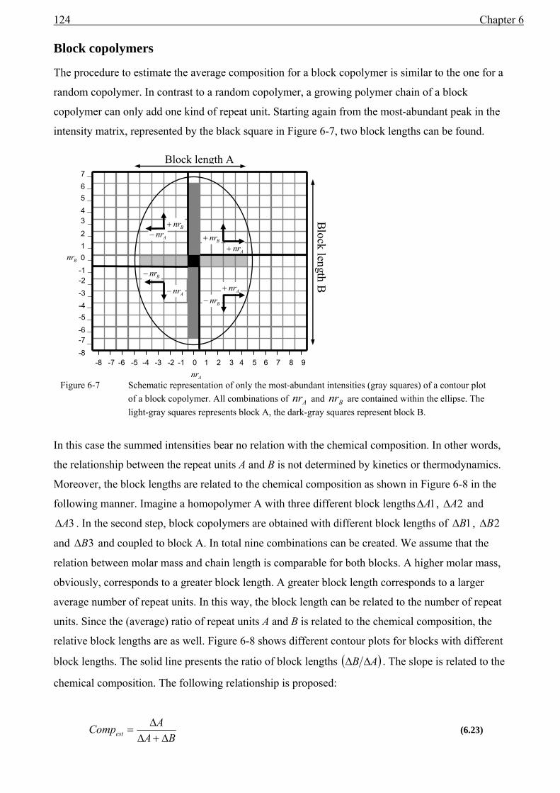
124 Chapter 6
Block copolymers
The procedure to estimate the average composition for a block copolymer is similar to the one for a
random copolymer. In contrast to a random copolymer, a growing polymer chain of a block
copolymer can only add one kind of repeat unit. Starting again from the most-abundant peak in the
intensity matrix, represented by the black square in Figure 6-7, two block lengths can be found.
In this case the summed intensities bear no relation with the chemical composition. In other words,
the relationship between the repeat units A and B is not determined by kinetics or thermodynamics.
Moreover, the block lengths are related to the chemical composition as shown in Figure 6-8 in the
following manner. Imagine a homopolymer A with three different block lengths 1A∆ , 2A∆ and
3A∆ . In the second step, block copolymers are obtained with different block lengths of 1B∆ , 2B∆
and 3B∆ and coupled to block A. In total nine combinations can be created. We assume that the
relation between molar mass and chain length is comparable for both blocks. A higher molar mass,
obviously, corresponds to a greater block length. A greater block length corresponds to a larger
average number of repeat units. In this way, the block length can be related to the number of repeat
units. Since the (average) ratio of repeat units A and B is related to the chemical composition, the
relative block lengths are as well. Figure 6-8 shows different contour plots for blocks with different
block lengths. The solid line presents the ratio of block lengths ( )AB ∆∆ . The slope is related to the
chemical composition. The following relationship is proposed:
BAACompest ∆+∆
∆= (6.23)
Figure 6-7 Schematic representation of only the most-abundant intensities (gray squares) of a contour plot of a block copolymer. All combinations of Anr and Bnr are contained within the ellipse. The light-gray squares represents block A, the dark-gray squares represent block B.
0 1 2 3 4
-5 -4 -3 -2 -1
5 6 7
-8 -7 -6
Bnr
Anr
Anr−
Bnr−
Anr+Bnr+
Anr+
Bnr−
Bnr+Anr−
0 1 2 3 4-5 -4 -3 -2 -1 5 6 7 8 9-8 -7 -6
Block length B
Block length A

Outlook and development 125
Where A∆ , and B∆ are the (maximum) length of the blocks in term of repeat units and estComp is
the average chemical composition.
The methods developed so far, were used to estimate the average chemical composition for random
and block copolymers. The two developed methods suffice to obtain a sufficiently reliable average
chemical composition to rule out the ghost peaks in the contour plots. The other topologies, such as
gradients, grafts, etc. can be classified in terms of “random-like” or more “blocky-like”.
After the “true” contour plot is obtained, the characteristics of the copolymer fingerprints will help
us to obtain information on the polymer topology.
6.4 characteristics of copolymer fingerprints
Before discussing the characteristics of copolymer fingerprints, the characteristics of copolymers
themselves should be understood, starting with a simple case, i.e. a block copolymer.
6.4.1 Block copolymers
A block copolymer can be characterized by the block lengths, which can be easily obtained from
the contour plot. The individual block-length distributions are the projection on the Anr -axis and
Bnr -axis for blocks A and B, respectively.
Anr
1A∆ 2A∆ 3A∆
1B∆
2B∆
3B∆ 11−=
∆∆
estCompAB
Bnr
Figure 6-8 Schematic representation of the relationship between block length and chemical composition. The slope of the solid lines or the block-length ratio ( )AB ∆∆ is directly related to the
i i

126 Chapter 6
( ) ∑=B
BAnr
nrnrAA IcnrBLD , and ( ) ∑=A
BAnr
nrnrBB IcnrBLD , (6.24)
Where BLD is the block length distribution and
BA nrnrIc , the corrected observed intensity.
If the random-coupling hypothesis holds, then the copolymer fingerprint can be interpreted as the
product of the two block-length distributions. This criterion is used to distinguish between random
and block copolymers and verifies whether the correct initial assumption was made to estimate the
average composition. The correlation coefficient of a block, BR , is defined as:
( ) ( ) ( ) ( )( )( )( )( ) ( ) ( ) ( )( ) ( )
2
,,
2 2,,
A BA B
A BA B
nr nrA A B B A A B B nr nr
B
nr nrA A B B A A B B nr nr
BLD nr BLD nr BLD nr BLD nr Ic IcR
BLD nr BLD nr BLD nr BLD nr Ic Ic
⋅ − ⋅ −=
⋅ − ⋅ −
∑
∑ ∑ (6.25)
Where 2 1BR = corresponds to a perfect block copolymer.
Even if the random-coupling hypothesis does not hold, the product of the two block-length
distributions will still give a higher correlation coefficient (for a block copolymer) than the random
copolymer test described below.
6.4.2 Random copolymers
As long as no composition drift occurs, a random copolymer can be characterized by a constant
composition along the chain-length distribution. To plot the composition versus the chain length, a
transformation of the intensity matrix is needed.
It is not correct to calculate the composition and chain length directly from the intensity matrix,
because of the non-linear spacing of the composition curves versus the number of repeat units. The
number of repeat-unit combinations having a composition between, for example, 50% ±0.5%, up to
100 repeat units equals 200, whereas for a composition of 35% ±0.5% this equals 92. The
relationship between composition and the number of repeat-unit combinations is shown in Figure
6-9. A bin size of one (a finite element of given dimensions, in this example one percent by one
repeat unit) does not contain equivalent number of combinations of the repeat units A and B at
different compositions.

Outlook and development 127
The correct transformation of the intensity matrix is obtained using the principle of latent variables.
Given a set of p variables, s smaller number of new variables are constructed that describe as much
of the information as possible (in statistical terms: as much variance as possible). New variables are
constructed in such a way that each of them contains unique information. The result will be a set of
uncorrelated or orthogonal variables. Note that for block copolymers the axes are already
orthogonal and, hence, this transformation is not needed.
If the composition is chosen to be the new latent variable (C) , the second variable (D) must be
oriented perpendicular to the composition axis to obtain an orthogonal system. The composition can
be described as function of the number of repeat units ( Anr and Bnr ) in the contour plot as:
Cnrnr AB +⋅= γ (6.26)
and the orthogonal axis becomes:
Dnr
nr AB +
−=
γ (6.27)
where γ is the slope, which can be calculated from the average composition. In order to understand
of the transformed intensity matrix, we recall the relationship between composition and chain
length as given by the Stockmayer equation8.
The Stockmayer equation describes the instantaneous relation between composition and chain
length, with the assumption that the reactivity of radicals depends only on the nature of the reactive
end, and with the kinetic effects of initiation and termination being neglected.
0
40
80
120
160
200
0 20 40 60 80 100
composition %
Cou
nts
Figure 6-9 The counts present the number of repeat-units combinations that were found within the bin size of one percent with a maximum of 100 repeat units. The irregular relation between the composition and the number of counts makes the direct transformation not suitable. Note that this curve is perfectly symmetrical around the 50 % composition.

128 Chapter 6
( ) ( ) ( ) ⎟⎟⎠
⎞⎜⎜⎝
⎛⋅⎟⎟⎠
⎞⎜⎜⎝
⎛⋅−⋅⋅
⋅−⋅
⋅−⋅⋅⋅⋅⎟⎟⎠
⎞⎜⎜⎝
⎛⋅⋅⎟
⎠⎞
⎜⎝⎛ −= dy
CCyL
CCLdLLLdLdyyLn
aveaveaveave κκπλλ 12exp
12exp,
2
(6.28)
( ) ( )1 21 4 1 1ave aveC C r rκ = − ⋅ ⋅ − ⋅ − ⋅ (6.29)
avey C C= − (6.30)
where aveC is the average overall composition, λ the degree of polymerization, 1r and 2r are the
reactivity ratios, y is the composition deviation, C the composition of an individual chain, and
( )yLw , the weight fraction of polymers of equal weight with lengths between L and dLL + and
composition deviations between y and dyy + . The chain length can be written as a function of C
and D (see appendix 6A)
2
2
1 γγγγ
+⋅+⋅+⋅−
=+=DDCCnrnrL BA (6.31)
Where C is the composition deviation expressed in terms of Anr and Bnr and D is a chain length
deviation expressed as the sum of Bnr and Anr⋅γ . Rewriting the composition in terms of C and D
(see appendix 6A) we obtain:
( )( ) ( )( )2
2
11
γγγγγ
⋅−⋅−⋅+−⋅++⋅
=DDCC
Cy (6.32)
Substitution of the expressions for y and L into equation (6.28) gives the instantaneous distribution
of chain compositions and chain lengths as function of C and D. When C is plotted versus D the
“flame” contour plot is obtained as seen in Figure 6-10.

Outlook and development 129
We conclude from the graphs in Figure 6-10 that a fully random copolymer results in a perfectly
symmetrical “flame” contour plot. The projection on the C-axis can be used to detect composition
γ⋅−= AB nrnrC
γA
BnrnrD +=
Anr
Bnr
Figure 6-10 Figure (a) shows the conventional presentation of the contour plot. Picture (b) shows the “flame” contour plot with orthogonal axes. (
1r =0.8, 2r =1.1,
aveC =0.6, λ =50)
(a)
(b)
130 Chapter 6
drift. The projection of Figure 6-10b will result in a Gaussian distribution. Any asymmetry of this
distribution can be directly related to composition drift. The asymmetry can be calculated from the
second order moment of the distribution (appendix 6D). The projection on the C-axis represents the
chemical-composition distribution and can be written in terms of Anr and Bnr :
max21A
D Cnr γγ
⎛ ⎞−= ⋅⎜ ⎟+⎝ ⎠
and 2
max21B
D Cnr γγ
⎛ ⎞⋅ += ⎜ ⎟+⎝ ⎠
(6.33)
Where the highest intensity of both the projection on the C-axis and D-axis are denoted as maxC and
maxD respectively.
The projection on the D-axis represents the chain length, which can be expressed in terms of Anr
and Bnr as well:
max21A
D Cnr γγ
⎛ ⎞−= ⋅⎜ ⎟+⎝ ⎠
and 2
max21B
D Cnr γγ
⎛ ⎞⋅ += ⎜ ⎟+⎝ ⎠
(6.34)
With the use of equations (6.33) and (6.34) the chemical-composition distribution (CCD) and the
chain-length distribution (CLD) can be obtained by the following equations.
( ) ( )( ) ( )
max2
max max
A
A B
D CnrCCD Cnr nr D C D C
γγ γ
−= =
+ − + ⋅ + (6.35)
( )( ) ( )2
max max21A B
D C D CCLD D nr nr
γ γ γ
γ
− + ⋅ += + =
+ (6.36)
The correlation coefficient of a random copolymer, RR , is defined as:
( ) ( ) ( ) ( )( )( )( )( ) ( ) ( ) ( )( ) ( )
2
,,
2 2,,
C DC D
R
C DC D
CCD C CLD D CCD C CLD D Ic IcR
CCD C CLD D CCD C CLD D Ic Ic
⋅ − ⋅ −=
⋅ − ⋅ −
∑
∑ ∑ (6.37)
Where the 2 1RR = corresponds to completely random.
In summary, various methods were discussed to correct the spectra to obtain the “true” contour
plots, as well as ways in which the contour plots should be plotted (finger print, flame). In this way

Outlook and development 131
a full CCD, CLD, or block-length distribution is the outcome of the developed program. The last
item which will be discussed is end group determination.
6.5 End-group analysis
The entire data set cannot distinguish between end groups, as it results in complete overlap. To
estimate the average composition, only the tops of the contour plot are used as described in section
6.3.4. This data set is very well suited for end-group determination. As discussed in section 5.1.2
the end-group-correlation function (ECF) is modified for copolymers and can be described by:
( )∑ ++⋅+⋅=MaxA
MinA
nr
nrendionBBAAend mmnrmnrmImECF
_
_
)( (6.38)
The obtained spectrum for the ECF contains an acceptably low number of possible end-group
masses, since the numbers of repeat units must meet the following criteria:
CompnrnrCompComp BAest ∆<− ),( (6.39)
( ) mmnrnrmm endBAcalcobserved ∆<− ,, (6.40)
Where Comp∆ is the composition error of the estimate average composition (section 6.3.4), and
m∆ the accuracy, typically ± 0.5 amu.
For random copolymers, the entire set of the so-called “tops of the contour plot” can be used for the
ECF. The ECF intensity is related to the probability of a particular end-group mass.
For block copolymers the “tops of the contour plot” exist of only one data point with a known
estimated composition. This data point is located at the maximum intensity of block length A and
block length B. Therefore all combinations of Anr and Bnr that pass both criteria will result in the
same ECF intensity or probability.
At this point the chemist has to reduce the remaining possible end-group masses. Note that once an
end-group mass is assigned, end-group masses that differ by the mass of the repeated units cannot
be distinguished from the previously assigned end-group mass.
After the end groups have been determined and the contour plots are made, the corresponding type
of topology can be determined.

132 Chapter 6
6.6 Determining types of topology
In this chapter the characteristics of the contour plots of block copolymers and random copolymers
were discussed. The obtained contour plots have to meet the following criteria:
Random copolymer: The transformation of the contour plot into latent variables (C, D)
results in results in a “flame” contour plot. The projection of the “flame” contour plot on the C and
D axis is used to confirm the random-copolymer topology.
Block copolymers: For block copolymers, the relation between the number of repeat units
and the composition is not known without any pre-knowledge. However depending on the relative
lengths of the two blocks, a more circular or elliptical contour can be recognized in the contour
plots. Projections of the contour plot on the number of repeat units A and B, is used to confirm the
block topology.
Alternating copolymers: The chemical-composition distribution, obtained from the “flame”
contour plot, is indicative for alternating copolymers, since an alternating copolymer has a very
narrow chemical-composition distribution.
Gradient copolymer: A gradient copolymer can be characterized as the intermediate form of
a random copolymer with a strong composition drift and a block copolymer. The asymmetry of the
projections on the axis of the “flame” contour plot is used to confirm the gradient topology.
In conclusion, the methods described above help us to extract “hidden” information from complex
spectra. Figure 6-11 shows the schematic overview of the followed procedure. Applications of these
methods will be illustrated by the examples of copolymerization of styrene-isoprene and butadiene-
styrene.
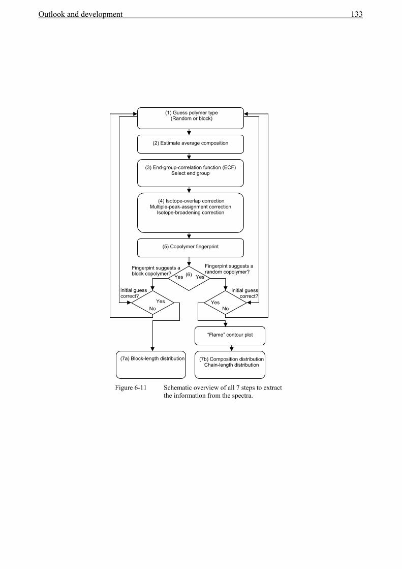
Outlook and development 133
(1) Guess polymer type (Random or block)
(2) Estimate average composition
(3) End-group-correlation function (ECF) Select end group
(4) Isotope-overlap correction Multiple-peak-assignment correction
Isotope-broadening correction
Fingerpint suggests a block copolymer?
Fingerpint suggests a random copolymer?
(5) Copolymer fingerprint
“Flame” contour plot
(7b) Composition distribution Chain-length distribution
(7a) Block-length distribution
Yes Yes No
Yes Yes
No
Figure 6-11 Schematic overview of all 7 steps to extract the information from the spectra.
(6)
initial guess correct?
Initial guess correct?
134 Chapter 6
6.7 Polystyrene-co-isoprene
Poly(styrene-block-polyisoprene) copolymer was prepared by anionic polymerization using sec-
butyllithium as the initiator as described elsewhere7. Four samples were withdrawn from the
reaction mixture after approximately 25, 50, 75, and 100% conversion of the isoprene monomer.
The spectra can be found in appendix 6B.
The analysis will be discussed step by step as explained in Figure 6-11.
Step 1 As an initial guess a block copolymer was taken. In this case the type of polymer was
already known.
Step 2 The initial compositions were calculated as described in section 6.3.4. The results are
reported in appendix 6C.
Step 3 The next step is to decide which end-group mass is correct. All four samples were subjected
to the ECF as can be seen in Table 18B (The results are listed in a table instead of a graph, since all
peaks have the same intensity originating for the black square in Figure 6-7). Sample 2 shows the
highest number of different end-group masses, due to the relative large composition error, as is
shown in Table 18B. A larger error in composition allows more combinations of repeat units A and
B to meet the criteria discussed in section 6.5.

Outlook and development 135
In this case sec-butyllithium was used as initiator which corresponds to a mass of 58.08 amu. Table
18A shows all possible end-group masses for the different samples. Note that 58 amu is the only
end-group mass which is found in each list of all samples. Some other frequently obtained end-
group masses (printed in bold) can be explained by the end-group mass 58 amu with small changes
in the chain composition (see Table 18C). Assuming that all end-group masses listed in Table 18C
belong to the end-group mass of 58.08 amu (sec-butyllithium), the majority of the end-group
masses can be explained.
Step 4 In order to see the effect of the corrections, different contour plots of sample 3 are shown in
Figure 6-12.
Sample 2 Mass (amu)
Sample 3 Mass (amu)
Sample 4 Mass (amu)
Sample 5 Mass (amu)
1.5 26 22 18
2 30 25.5 21.5
25.5 58 26 22
26 62 58 54
29.5 66 61.5 57.5
30 94 62 58
33.5 98 94 90
34 102 122
37.5
38
58
61.5
62
65.5
66
69.5
70
94
97.5
98
101.5
102
105.5
106
Sample number 2 3 4 5 Estimate average-composition (%)
41 45 51 55
Corrected composition
23 34 48 58
Error % 19 11 4 3
End-group masses (amu)
Exchange of number of Styrene units
Exchange of number of Isoprene units
58.08 0 094.08 1 -122.08 -1 126.02 1 -290.14 -1 262.03 2 -354.13 -2 3
Table 18B The error in the initial estimated average composition.
Table 18C Possible end-group masses due to the exchange of repeat mass units starting from 58 amu.
Table 18A A list of all possible end-group-masses. Bold numbers correspond to the end-group-mass of 58 amu with zero, one or two units of styrene or isoprene (see table 4C).
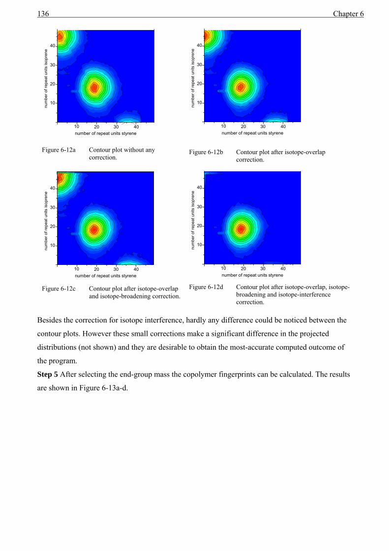
136 Chapter 6
Besides the correction for isotope interference, hardly any difference could be noticed between the
contour plots. However these small corrections make a significant difference in the projected
distributions (not shown) and they are desirable to obtain the most-accurate computed outcome of
the program.
Step 5 After selecting the end-group mass the copolymer fingerprints can be calculated. The results
are shown in Figure 6-13a-d.
40302010
40
30
20
number of repeat units styrene
num
ber o
f rep
eat u
nits
isop
rene
10
40302010
40
30
20
number of repeat units styrene
num
ber o
f rep
eat u
nits
isop
rene
10
40302010
40
30
20
number of repeat units styrene
num
ber o
f rep
eat u
nits
isop
rene
10
40302010
40
30
20
number of repeat units styrene
num
ber o
f rep
eat u
nits
isop
rene
10
Figure 6-12b Contour plot after isotope-overlap correction.
Figure 6-12d Contour plot after isotope-overlap, isotope-broadening and isotope-interference correction.
Figure 6-12a Contour plot without any correction.
Figure 6-12c Contour plot after isotope-overlap and isotope-broadening correction.

Outlook and development 137
Step 6 and 7 The initial assumption of a block copolymer can be verified by reconstructing the
contour plot of the block length distributions. The correlation between the original contour plot and
the reconstructed contour plot is used to judge if the initial assumption was correct. The calculated
block lengths are depicted in Figure 6-14. Correlation coefficients exceeding 0.998 where obtained
for samples 1 through 4. In case of a correlation coefficient less then 0.975 (5% of unexplained
variation) the entire cycle would be repeated to test the alternative topology (random copolymer).
40302010
40
30
20
number of repeat units styrene
num
ber o
f rep
eat u
nits
isop
rene
10
40302010
40
30
20
number of repeat units styrene
num
ber o
f rep
eat u
nits
isop
rene
10
40302010
40
30
20
number of repeat units styrene
num
ber o
f rep
eat u
nits
isop
rene
10
40302010
40
30
20
number of repeat units styrene
num
ber o
f rep
eat u
nits
isop
rene
10
Figure 6-13b Sample 3, approximately 50% conversion of isoprene.
Figure 6-13d Sample 5, approximately 100% conversion of isoprene.
Figure 6-13a Sample 2, approximately 25% conversion of isoprene.
Figure 6-13c Sample 4, approximately 75% conversion of isoprene.

138 Chapter 6
Starting from a complex copolymer spectrum, the entire distribution has been reduced to only two
simple graphs as depicted in Figure 6-14.
A completely different problem associated with MALDI-TOF-MS data is the need to apply a
correct baseline subtraction (section 2.3.1). Extraction of the block-length distribution of the
precursor block with increasing conversion of the second block, was used as a direct method to
elucidate which baseline method resulted in the most consistent precursor block-length
distributions. The results of both methods are shown in section 2.3.1. All spectra throughout this
thesis were processed by the valley-to-valley method.
Figure 6-14 The block-length distribution of the polystyrene and polyisoprene.
0 5 10 15 20 25 30 35 40 45 500.00
0.02
0.04
0.06
0.08
0.10
0.12
0.14
Inte
nsity
(a.u
.)
number of repeat units isoprene
sample 1 sample 2 sample 3 sample 4
5 10 15 20 25 30 35 40
0.00
0.02
0.04
0.06
0.08
0.10
Inte
nsity
(a.u
.)
Number of repeat units
sample 1 sample 2 sample 3 sample 4 Homopolymer
number of repeat units styrene
(A) (B)

Outlook and development 139
6.8 Polystyrene-gradient-butadiene
The program calculates the correlation coefficient for a block and a random copolymer. We can use
these “extremes” to elucidate other topologies, for example a gradient copolymer.
A gradient copolymer was prepared by anionic polymerization of butadiene and styrene. Such a
gradient copolymer can be obtained as long as the composition drift be can regulated to some extent
during a living polymerization. Moreover, the system has to meet two criteria. First, the cross
propagation in both directions should neither be too slow nor too fast. A too slow cross propagation
leads to the formation of block structures. On the other hand, a too fast cross propagation leads to
an alternating copolymer. Secondly, the two homopropagation rate constants should not differ
orders of magnitude. The reactivity of the anions can be influenced by lewis bases, such as
N,N,N',N'-tetramethylethylenediamine (TMEDA)9,10, to meet the previously mentioned criteria.
6.8.1 Experimental section
The poly(styrene-gradient- butadiene) copolymer was prepared by anionic polymerization using
sec-butyllithium (Acros, 1.3 M solution in cyclohexane/hexane (97.8/30.1 mL)) as the initiator.
Reactions were carried out in a 2-L stainless-steel autoclave reactor under a nitrogen atmosphere
using cyclohexane (VWR, high purity) as a solvent. Monomers and solvent were passed over an
activated alumina column prior to polymerization. The autoclave reactor was loaded with 989 g of
cyclohexane and heated to 40°C. A mixture of 50.2 g styrene (VWR, 99%), 26.2 g butadiene (Shell
Chemicals, 99.5%), and 67.7 mL 0.028 M sec-butyllithium and 2.239 g of N,N,N',N'-
tetramethylethylenediamine (TMEDA, VWR, 99%) solution in cyclohexane were added to the
autoclave reactor. Within 15 minutes full conversion was achieved, since all samples drawn from
the reaction mixture after 15 minutes showed 100% conversion. All samples were terminated by
quenching in an excess of methanol.
6.8.2 MALDI-TOF-MS Analysis
Each step of the program is discussed in section 6.7, therefore only the outcome of the program is
discussed here. A gradient copolymer can be seen as an “intermediate” between a block copolymer
and a random copolymer and it will fail both tests to detect the random or block topology.
Therefore the contour plots in both the block and random formats, are depicted.

140 Chapter 6
Although it is obvious that neither of these images obey the random or block copolymer topology,
the projections on the axes were performed to confirm this mathematically.
Figure 6-16 and Figure 6-17 represent the projected distributions on the axes. The relatively low
correlation coefficients and the relatively large skewness value of the composition distribution
confirmed the gradient topology. Note that this gradient copolymer shows more resemblance with a
random copolymer than with a block copolymer. Using the correlation coefficients, this copolymer
can be characterized as a 33% block copolymer and a 67% random copolymer.
Figure 6-16 (a) The chemical-composition distribution and (b) the chain length distribution of the butadiene-gradient-styrene copolymer assuming a random copolymer structure. A correlation coefficient of 0.953 (10% unexplained variance) was obtained. CCDτ = 20%.
0 10 20 30 40 50 60 700.0
0.2
0.4
0.6
0.8
1.0
rela
tive
inte
nsity
Chain length 0.0 0.2 0.4 0.6 0.8 1.0
0.0
0.2
0.4
0.6
0.8
1.0
rela
tive
inte
nsity
Butadiene fraction(%)
(a) (b)
Figure 6-15 Contour plots of a poly(styrene-gradient-butadiene)polymer. The dashed line indicates “the path” of a gradient copolymer.
60
50
-27-17-731323
40
20
10
Anr
AB
nrnrγ
+
40302010
40
30
20
10
Bnr
B Anr nr γ− ⋅
Block contour plot Random contour plot

Outlook and development 141
Figure 6-17 (a) The butadiene block-length distribution and (b) the styrene block-length distribution of the butadiene-gradient-styrene copolymer assuming a block-copolymer structure. A correlation coefficient of 0.903 (19% unexplained variance) was obtained.
0 5 10 15 20 25 300.0
0.2
0.4
0.6
0.8
1.0
Rel
ativ
e in
tens
ity
number of repeat units butadiene
-5 0 5 10 15 20 25 30 35 400.0
0.2
0.4
0.6
0.8
1.0
Rel
ativ
e in
tens
ity
number of repeat unit styrene
(a) (b)

142 Chapter 6
6.9 Conclusions
The interpretation of copolymer spectra obtained by MALDI-TOF-MS is no longer laborious and
time consuming with the help of our program. In essence, for a copolymer consisting of two
monomers, the entire spectrum is “digitized” in a contour plot representation. This representation
can elucidate, directly or indirectly, the relationship between the molar mass and the composition of
the polymer chains expressed as the number of repeat units A and B. The criteria discussed in
section 6.6 reveal the topology of the copolymer for a random, gradient, block, and alternating
copolymer.
A long-lasting conflict concerning baseline subtractions in MALDI-TOF-MS is clarified. The so-
called valley-to-valley method resulted in the most appropriate obtained values of the precursor
block length distribution of a block copolymer, providing direct evidence of the correct baseline
subtraction method.
To obtain the best contour plot, a number of corrections have to be made. These corrections are
mainly mathematical in nature. These corrections allow elucidation of the most appropriate
baseline-subtraction method. The corrections improve the quality of the program outcome
significantly. Nevertheless, the differences are small and not always visually noticeable.
We hope that this work will contribute to a more systematic method for processing the MALDI-
TOF-MS spectra of (co)polymer. The need for such standardized methods has been underlined by a
round robin test11 where a homopolymer end-group analysis is carried out. A round-robin test
involving copolymers by MALDI-TOF-MS has not yet been carried out.

Outlook and development 143
Reference List 1. Yergey, J. A. Int. J. Mass Spectrom. Ion Phys 1983, 52, 337-349.
2. Suddaby, K. G.; Hunt, K. H.; Haddleton, D. M. Macromolecules 1996, 29, 8642-8649.
3. Wilczek-Vera, G.; Yu, Y.; Waddell, K.; Danis, P. O.; Eisenberg, A. Rapid commun. Mass Spectrom. 1999, 13 (9), 764-777.
4. Wilczek-Vera, G.; Danis, P. O.; Eisenberg, A. Macromolecules 1996, 29 (11), 4036-4044.
5. Wilczek-Vera, G.; Yu, Y.; Waddell, K.; Danis, P. O.; Eisenberg, A. Macromolecules 1999, 32 (7), 2180-2187.
6. van Rooij, G. J.; Duursma, M. C.; de Koster, C. G.; Heeren, R. M. A.; Boon, J. J.; Schuyl, P. J. W.; van der Hage, E. R. E. Anal. Chem. 1998, 70 (5), 843-850.
7. Willemse, X. E.; Staal, B. B. P.; Donkers, E. H. D.; van Herk, A. M. Macromolecules 2004.
8. Stockmayer, W. H. The Journal of Chemical Physics 2004, 13 (6), 199-207.
9. Collum, D. B. Acc. Chem. Res. 1992, 25, 448-454.
10. Melenevskaya, Y. Y.; Zgonnik, V. N.; Denisov, V. M.; Dolinskaya, E. R.; Kalnin'sh, K. K. Polymer Science U. S. S. R. 1980, 21, 2215-2224.
11. Guttman, C. M.; Wetzel, J.W.; Wallace, W.E.; Blair, W.R.; Goldschmidt, R.M.; Vanderhart, D.L.; Fanconi, B.M.; . Polym. Prepr. 2000, 41, 678-679.

144 Chapter 6
Appendix 6A The instantaneous distribution of chain compositions and chain lengths can be described by the Stockmayer equation with the assumption that the reactivity of radicals depends only on the nature of its reactive end and the kinetic effects of initiation and termination are neglected.
( ) ( ) ( ) ⎟⎟⎠
⎞⎜⎜⎝
⎛⋅⎟⎟⎠
⎞⎜⎜⎝
⎛⋅−⋅⋅
⋅−⋅
⋅−⋅⋅⋅⋅⎟⎟⎠
⎞⎜⎜⎝
⎛⋅⋅⎟
⎠⎞
⎜⎝⎛ −= dy
CCyL
CCLdLLLdLdyyLn
aveaveaveave κκπλλ 12exp
12exp,
2
(A6-1)
( ) ( )1 21 4 1 1ave aveC C r rκ = − ⋅ ⋅ − ⋅ − ⋅ (A6-2)
aveCCompy −= (A6-3)
where aveC is the average overall composition, λ the degree of polymerization, 1r and 2r the reactivity ratios, y the composition deviation and C the composition of an individual chain and ( )yLn , the number fraction of polymers with lengths between L and dLL + and composition-
deviations between y and dyy + . The direction of the new axis is chosen parallel to the slope of the contour plot (related to the average composition) and perpendicular to the latter axis to obtain a orthogonal axis. The average composition can be described as function of Anr and Bnr in the contour plot as:
Cnrnr AB +⋅= γ (A6-4)
and the orthogonal axis becomes:
Dnr
nr AB +
−=
γ (A6-5)
where γ is the slope which can be calculated from the average composition ( )γ+= 11aveC . The value C is the composition-deviation expressed in terms of repeat units A and B and D is a certain chain length expressed as the sum of Bnr plus Anr⋅γ . Writing the repeat units A and B as function of C and D results in:
2
2
1 γγ+
+⋅=
CDnrB (A6-6)
( )21 γ
γ+−⋅
=CDnrA (A6-7)
Rewriting the chain length in terms of C and D:
2
2
1 γγγγ
+⋅+⋅+⋅−
=+=DDCCnrnrL BA (A6-8)
Rewriting the composition in terms of C and D:
11+
−+
=−=γBA
Aave nrnr
nrCCompy (A6-9)

Outlook and development 145
( )( ) ( )( )2
2
11
γγγγγ
⋅−⋅−⋅+−⋅++⋅
=DDCC
Cy (A6-10)
Substitute A6-8 and A6-10 into A6-1 and the number fraction is obtained as function of C and D. Note that the molar mass can be written as a function of C and D:
( ) ( )⎟⎟⎠
⎞⎜⎜⎝
⎛+−⋅
⋅+⎟⎟⎠
⎞⎜⎜⎝
⎛+
+⋅⋅= 22
2
11,
γγ
γγ CDmCDmDCM BA (A6-11)
After rearrangement:
( ) ( )⎟⎟⎠
⎞⎜⎜⎝
⎛+⋅⋅
+⋅+⎟⎟
⎠
⎞⎜⎜⎝
⎛+⋅⋅−⋅
⋅=BABA
AB
mmM
mmmm
CDγγγ
γγγ 21 (A6-12)
It can be seen that the intercept is indicative for the molar mass in the contour plot of C versus D. Appendix 6B The spectra of the poly(styrene-co-isoprene) samples.
1577 2339 3102 3864 4627Mass (m/z)
% In
tens
ity
Sample 3
Mass (m/z)
Sample 2
1625 2181 2737 3294 3850
% In
tens
ity
Sample 2
1577 2339 3102 3864 4627Mass (m/z)
% In
tens
ity
Sample 3
Mass (m/z)
Sample 2
1625 2181 2737 3294 3850
Sample 2
1625 2181 2737 3294 3850
% In
tens
ity
Sample 2
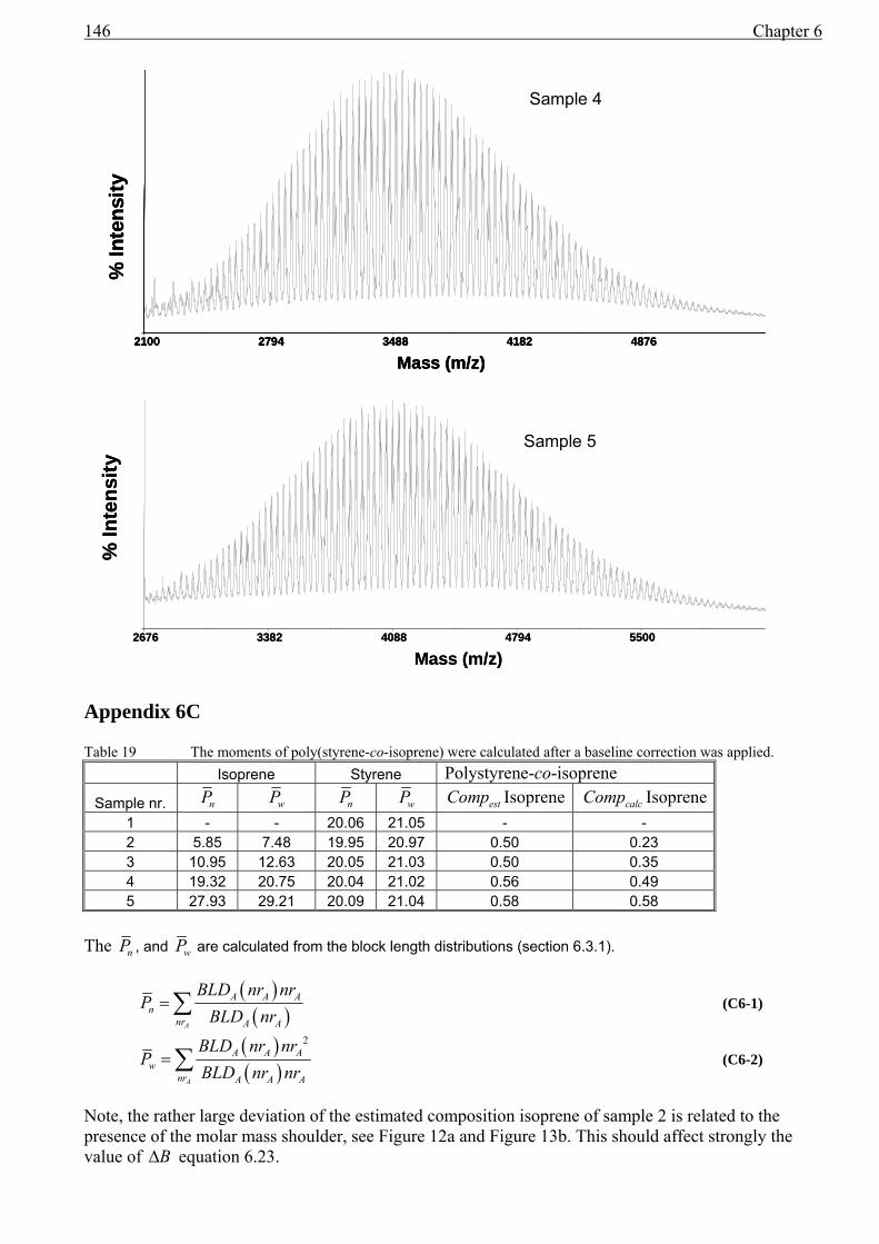
146 Chapter 6
Appendix 6C Table 19 The moments of poly(styrene-co-isoprene) were calculated after a baseline correction was applied. Isoprene Styrene Polystyrene-co-isoprene
Sample nr. nP wP nP wP estComp Isoprene calcComp Isoprene
1 - - 20.06 21.05 - - 2 5.85 7.48 19.95 20.97 0.50 0.23 3 10.95 12.63 20.05 21.03 0.50 0.35 4 19.32 20.75 20.04 21.02 0.56 0.49 5 27.93 29.21 20.09 21.04 0.58 0.58
The nP , and wP are calculated from the block length distributions (section 6.3.1).
( )( )A
A A An
nr A A
BLD nr nrP
BLD nr=∑ (C6-1)
( )( )
2
A
A A Aw
nr A A A
BLD nr nrP
BLD nr nr=∑ (C6-2)
Note, the rather large deviation of the estimated composition isoprene of sample 2 is related to the presence of the molar mass shoulder, see Figure 12a and Figure 13b. This should affect strongly the value of B∆ equation 6.23.
2676 3382 4088 4794 5500
Mass (m/z)
% In
tens
ity
2100 2794 3488 4182 4876
Mass (m/z)
% In
tens
ity
2676 3382 4088 4794 5500
Mass (m/z)
% In
tens
ity
2100 2794 3488 4182 4876
Mass (m/z)
% In
tens
ity
2100 2794 3488 4182 4876
Mass (m/z)
% In
tens
ity
Sample 5
Sample 4
Outlook and development 147
Appendix 6D The asymmetry of any distribution can be calculated via the statistical moments. The first moment of the distribution represents the mean value( n ):
I
nn
= ∑∑
(D6-1)
Where I is the normalize distribution as function of n. The second moment represents the standard deviation (σ ): ( )22 n n Iσ = −∑ (D6-2)
The third moment is related to the skewness (τ ):
( )333/ 2
1 n n Iτσ
= −∑ (D6-3)
The skewness of a distribution is a measure of the composition drift. No composition drift leads a value of zero.

148 Chapter 6

Outlook and development 149
Chapter 7
7 Outlook and development
Matrix-Assisted Laser Desorption/Ionization Time-of-Flight Mass Spectrometry (MALDI-TOF-
MS) of polymers is only a niche in the mass spectrometry market in comparison with clinical and
biochemical applications. The main driving force of technological development in MALDI-TOF-
MS is automation of high-throughput screenings. The benefits of these developments for polymer
analysis are limited.
The more interesting areas for polymer analysis are related to sample preparation, new types of
MALDI interfaces which allow hyphenation, and software development.
The development of new matrices is a continuous process as shown by some recent publications1,2.
However, as long as there is no fundamental understanding of the role of the matrix in the MALDI
process, the discovery of new matrices will proceed slowly. A new trend in sample preparation is
solvent-free sample deposition. The sample and the matrix are mixed as powders and pasted on to
the target. No fundamental difference was found in comparison with solvent based deposition.
Considerable progress has been made in the design of analyzers with the introduction of orthogonal
acceleration (oa). The main advantage of the oa-analyzer is the possible hyphenation with liquid
chromatography techniques. An additional advantage of oa-analyzers is the possibility to perform
MS/MS experiments. Particularly successful are the hybrid Quadrupole Time-of-Flight (Q-TOF)
mass spectrometers and the recently introduced MALDI-Q-TOF combination. A drastic mass-

150 Chapter 7
resolution improvement can be expected from the coupling of MALDI with a Fourier Transform
Ion Cyclotron Resonance Mass Spectrometer (FT-ICR-MS).
Fast online analysis and high-resolution measurements leave data interpretation as the limiting step
in mass spectrometry. Not only fast computers are needed to process the data, also large capacities
for data storage are needed. The use of “smart” software can help to extract only the essential
information from acquired spectra. In case of end-group analysis of polymers, the end-group
correlation function (ECF) can be seen as an end-group finger print of the entire spectrum. The
same holds for copolymer systems, where the intensity matrix for a given total end-group mass
contains all the information encrypted in the complex spectrum.
Despite all the promising techniques and developments, the main shortcomings of MALDI (the
non-quantitative intensities and the mass discrimination in case of broad polymer distributions) will
always necessitate the use of additional separation methods.
Reference List
1. Rajin, N. P.; Mirza, S. P.; Vairamni, M.; Ramulu, A. R.; Pard-Hasaradhi, M. Rapid commun.
Mass Spectrom. 2001, 15, 1884.
2. Brown, T.; Cliptson, N. C.; Simjee, N.; Luftmann, H.; Hungerbühler, H.; Drewllo, T. Int. J.
Mass Spectrom. 2001, 210/211, 249.

Glossary 151
Glossary of Symbols and Abbreviations ηsp Specific viscosity
y Composition deviation TCE functionality of 2,2,2-trichloroethanol SEC Size-Exclusion Chromatography SEC Size Exclusion Chromatography RALS Right-Angle Light Scattering RAFT Reversible Atom Fragmentation Transfer p-TsCl p-toluenesulphonyl chloride PPI N-npentyl-2-pyridylmethanimine PMDETA N,N,N′,N″,N″-pentamethyldiethylenetriamine PDI Polydispersity index PDA Photodiode Array NMP Nitroxide Mediated Polymerization MMD Molar Mass Distribution MMCCD Molar-Mass-Chemical-Composition Distribution MMA Methylmethacrylate MALDI-TOF-MS Matrix-Assisted-Laser-Desorption Ionization Time-of-Flight Mass
Spectrometry L Chain length K Mark-Houwink constant IP Pressure difference across the bridge IBC Isotope-broadening correction factor FTIR Fourier-Transform Infrared Spectroscopy f Correction factor for ( )Mn to ( )Mw log distribution.
ESI Electrospray ionization ECF End-group-correlation function ECF End-group Correlation Function EBriB Ethyl 2-bromoisobutyrate DRI Differential Refractive Index DP Viscosity signal DP Differential pressure within the bridge DCTB Trans-2-[3-(4-tert-butylphenyl)-2-methyl-2-propenylidene]malononitrile CPR Control Radical Polymerization CLD Chain-length distribution CCD Chemical-composition distribution C, D Latent variables to describe the chain length and chemical composition b Path length of the cell ATRP Atom-Transfer Radical Polymerization amu Atomeric mass units ACF Autocorrelation function ACF Auto Correlation Function
Am , Bm Molar mass of the monomers
Anr , Bnr Number of repeat units
1endm , 2endm Mass of one of the end groups of a polymer chain
minm , maxm Lower and upper limit masses of the isotope distribution
1µ , 1µ Corresponding masses of the most abundant isotopes
( )∑ AI , ( )∑ BI Total added intensity of repeat units A or B relative to the highest observed intensity
A∆ , B∆ Block length in number of repeat units A or B

152 Glossary
1r , 2r Reactivity ratios
2A , 3A Second-, and third-order virial coefficients
Anr∆ , Bnr∆ Number of repeat unit differences (integers)
ANr∆ , BNr∆ Number of repeat unit differences (non integers)
z Charge state e Charge of an electron
V∆ Electric potential difference m Mass (amu) ν Velocity of an ion
L Length of the flight tube t Flight time
0t Time when the ablating laser pulse hits the target
t∆ Time difference across a peak at full-width-half-height m∆ Mass difference expressed in amu
A Integrated or summed area of a MALDI spectrum
( )I t Observed intensity of the spectrum
exV Exclusion volume
SECK Distribution coefficient
pV Total pore volume
pM Most probable molar mass
nM Number averaged molar mass
wM Weight averaged molar mass
zM z-averaged molar mass
2adjR Adjusted correlation coefficient
( )hV hydrodynamic volume
[ ]η Intrinsic viscosity
v Retention volume α Mark-Houwink constant
visk Calibration factors of the pressure transducers
0η Viscosity of the solvent
frφ Flow-fraction correction factor
( )θR∆ Excess Rayleigh ratio
θ Scattering angle c Concentration of the analyte in SEC
( )θP Dissymmetry factor
LSK Light scattering constant
0n Refractive index of the eluent
0λ Wavelength in vacuum of the vertically polarized incident light
AN Avogadro number
( )dcdn Specific refractive-index increment
ε Molar absorption coefficient
( )vy Response of the DRI detector at an elution volume v
( )λ,vy Response of the PDA detector at an elution volume v and a given wavelength (λ )

Glossary 153
injV Injection volume
DRIk DRI calibration factor
PDAk PDA calibration factor
σ Dispersion constant
( )vG Gaussian band-broadening function
( )1vw Unbiased true MMD
DRI LSIDD − Inter-detector delay of the DRI and the LS
DRI DPIDD − Inter-detector delay of the DRI and the DP
DRI UVIDD − Inter-detector delay of the DRI and the UV
( )Mn Number distribution
( )Mw Weight distribution
( )Mw log Logarithmic weight distribution (SEC)
)(vR Normalized concentration signal
σ Dispersion constant, standard deviation
obsm Observed mass of a peak in the MALDI-TOF-MS spectrum
ionm Mass of the adduct
endm Mass of the total end group mass
MaxAnr _ Maximum number of repeat units
HRECF High resolution End-group Correlation Function
repm Mass step size
calcm Calculated mass of the most abundant isotope
),( BA nrnrI Intensity matrix
)(mI Original peak intensity
mI Corrected peak intensity
( )BABA nrnrmnrnrP ,,, Percentage relative to the most abundant peak of the corresponding isotope distribution of a given number of repeat units at a given mass ( )BA nrnrm , .
abdm Mass of the most abundant isotope
m∆ Mass interval expressed in amu
Im∆ Mass interval of the isotope distribution expressed in amu
mI∆ Mass interval expressed in terms of ANr∆ and BNr∆
( )BA nrnrIc , Corrected intensity matrix of a system subject to isotope interference
estcomp Estimated average composition
BLD Block length distribution
BR Correlation coefficient of a block
γ Slope of a curve in a copolymer fingerprint
aveC Average overall composition
λ Degree of polymerization C Composition of an individual chain
( )yLw , Weight fraction of polymers of a given chain length and chemical composition deviation
RR Correlation coefficient of a random copolymer
n Mean value of a distribution τ Skewness of a distribution
Summary 154
Summary
Over the past decade, mass spectrometry (MS) has revolutionized the characterization of synthetic
polymers. Moreover, with the introduction of matrix-assisted-laser-desorption ionization time-of-
flight mass spectrometry (MALDI-TOF-MS), it has become possible to obtain the polymer
characteristics (end groups, molar-mass distribution, topology etc.) However, the outcome of a
single measurement, a MALDI spectrum, needs to be transformed to visualize the polymer
characteristics since they are enclosed in the spectrum. The work described in this thesis, contains
the development of methods to extract and visualize all polymer characteristics embedded in a
spectrum.
One of the most well known characteristics of polymers is the molar-mass distribution.
Traditionally, the MMD is determined by size exclusion chromatography (SEC). SEC is a relative
method and is subject to column band-broadening. The effect of band broadening on the MMD can
be diminished by the use of molar-mass dependent detectors, such as light scattering and
viscometry. However, a setup with detectors connected parallel/serial requires accurate handling of
the large number of parameters to obtain a reliable absolute MMD (Chapter 3).
The limiting factor to obtain the MMD with MALDI is the occurrence of mass discrimination.
Polymers with a polydispersity index (PDI) larger than 1.2 show, in many cases, an underestimation
of the MMD towards the high molar mass range. For (polystyrene) polymers with a PDI larger than
1.2 the use of a relatively new matrix, matrix trans-2-[3-(4-tert-Butylphenyl)-2-methyl-2-
propenylidene]malononitrile (DCTB), significantly reduces mass discrimination in comparison with
conventional matrices. An attractive method to avoid mass discrimination is the use of a SEC
separation prior to MALDI measurement. This SEC separation supplies narrow molar-mass
fractions (PDI<1.2), these fractions can be measured by MALDI without mass discrimination.
Since MALDI-TOF-MS allows the determination of the mass of polymer chains with a high
accuracy, this technique is very well suited for total end-group-mass analysis. Our method for end-
group-mass analysis provides an end-group-mass spectrum where all end-group-masses within the
sample are present. The end-group-mass spectrum can be used to e.g. reveal the initiator
functionality or to distinguish between end-group-masses of nearly the same mass (Chapter 5).
The analysis and interpretation of MALDI spectra, in particular of copolymers, is a time consuming
task. The in-house developed software based on the methods described in this thesis, digitizes a
spectrum in terms of monomer repeat units. The representation of such a digitized spectrum is

155 Summary
called a copolymer fingerprint. The shape of a copolymer fingerprint reveals the copolymer
topology (random, block, alternating or gradient) (Chapter 6).
The aim of this work is the development of a method to extract all (co)polymer characteristics
enclosed from a MALDI spectrum, with absolute minimum prior knowledge. The use of the method
we developed offers a powerful and fast tool to obtain detailed information about the (co)polymer
characteristics.
Samenvatting 156
Samenvatting Sinds begin jaren negentig heeft massaspectrometrie (MS) zich een onmisbare positie verworven op
het gebied van de synthetische polymeerkarakterisering. De kracht van de MS techniek zit vooral in
de grote precisie waarmee de massa’s van individuele polymeerketens kunnen worden bepaald. Een
belangrijke plaats om verdelingen van polymeerketens te bepalen, wordt hedendaags ingenomen
door Matrix Assisted Laser Desoption/Ionization (MALDI). Echter het resultaat van een meting is
nog niet “vertaald” in de karakteristieken van het polymeer. Via het werk beschreven in dit
proefschrift, is getracht een generieke methode te ontwikkelen om alle karakteristieken, opgeslagen
in een MALDI spectrum, hanteerbaar en zichtbaar te maken.
Een van deze karakteristieken van polymeren is de molmassaverdeling. Traditioneel wordt deze
veelal bepaald met Size Exclusion Chromatography (SEC). SEC is een relatieve methode en is o.a.
onderhevig aan kolom verbreding wat kan worden ondervangen door het gebruik van molmassa
afhankelijke detectoren, zoals licht verstrooiing en viscosimetrie. Echter, de moeilijkheid van het
koppelen van detectoren in serie/parallel behelst een nauwkeurig inzicht in het grote aantal
parameters om tot een zo absoluut mogelijke molmassaverdeling te komen (hoofdstuk 3).
Een beperkende factor in het gebruik van MALDI voor het bepalen van de molmassaverdeling, is
de zogenoemde massadiscriminatie. Polymeren met een polydispersiteit index (PDI) groter dan 1.2
vertonen veelal een onderschatting van de hoogmoleculaire kant van de molmassa verdeling. De
kwantificering van massadiscriminatie toont aan, dat het gebruik van de relatief nieuwe matrix
DCTB een aanzienlijke verbetering vertoont voor het verkrijgen van de molmassaverdeling met een
PDI groter dan 1.2.
Een zeer aantrekkelijk alternatief is de combinatie van MALDI en SEC. SEC levert een smalle
molmassaverdeling die, zonder enige massadiscriminatie, gemeten kan worden met MALDI
(hoofdstuk 4).
De grote precisie waarmee MALDI-TOF-MS de massa van polymeerketens bepaalt, leent zich voor
de totale eindgroep massa analyse. De ontwikkelde procedures resulteren in een eindgroep spectrum
waarin alle informatie van aanwezige eindgroepen wordt weergegeven. De verkregen informatie
over de eindgroepen kan worden gebruikt om bijvoorbeeld de initiator functionaliteit te herleiden.
Tussen eindgroepen met nagenoeg dezelfde massa kan, tot op zekere hoogte, het onderscheid
worden gemaakt met behulp van een aangepaste procedure (hoofdstuk 5).
Het analyseren en interpreteren van MALDI spectra, in het bijzonder van copolymeren, is een
lastige en tijd rovende puzzel. Met behulp van de in dit proefschrift ontwikkelde software wordt het
spectrum gedigitaliseerd in termen van monomeer eenheden. De presentatie van een MALDI

157 Samenvatting
spectra op deze manier wordt een copolymere vingerafdruk genoemd. De vorm van deze
“vingerafdruk” is karakteristiek voor het type copolymeer (random, blok, altenerend of gradiënt) en
daarmee kan het type copolymeer direct worden toegekend (hoofdstuk 6).
De doelstelling van dit werk is de ontwikkeling van een methode om alle (co)polymeer
karakteristieken opgesloten in een MALDI spectrum er uit te extraheren met een minimale
hoeveelheid voorkennis. Het gebruik van de door ons ontwikkelde methode, bied een krachtige en
snelle manier om de (co)polymeer karakteristieken te verkrijgen.

Scientific papers 158
Scientific papers Bastiaan B. P. Staal1; Rajan Venkatesh1; Sreepadaraj Karanam; Bert Klumperman; A study to reveal the initiator functionality of trichloroethanol in ATRP of PMMA by end-group analysis with MALDI-TOF-MS, in preparation. Willemse, Robin X. E.; Staal, Bastiaan B. P.; Donkers, Ellen H. D.; Van Herk, Alex M. Copolymer Fingerprints of Polystyrene-block-polyisoprene by MALDI-ToF-MS; Macromolecules, (2004), 37(15), 5717-5723 Willemse, Robin X. E.; Staal, Bastiaan B. P.; van Herk, Alex M.; Pierik, Sebastiaan C. J.; Klumperman, Bert. Application of Matrix-Assisted Laser Desorption Ionization Time-of-Flight Mass Spectrometry in Pulsed Laser Polymerization; Macromolecules, (2003), 36(26), 9797-9803 Venkatesh, Rajan; Staal, Bastiaan B. P.; Klumperman, Bert; Monteiro, Michael J. Characterization of 3 and 4-Arm Stars from Reactions of Poly(butyl acrylate) RAFT and ATRP Precursors. Macromolecules (2004), 37(21), 7906-7917 Willemse, Robin X. E.; Staal, Bastiaan B. P.; van Herk, Alex M.; Pierik, Sebastiaan C. J.; Klumperman, Bert. Application of Matrix-Assisted Laser Desorption Ionization Time-of-Flight Mass Spectrometry in Pulsed Laser Polymerization. Chain-Length-Dependent Propagation Rate Coefficients at High Molecular Weight: An Artifact Caused by Band Broadening in Size Exclusion Chromatography? Macromolecules (2003), 36(26), 9797-9803 Vander Heyden, Y.; Popovici, S.-T.; Staal, B. B. P.; Schoenmakers, P. J. Contribution of the polymer standards' polydispersity to the observed band broadening in size-exclusion chromatography; Journal of Chromatography, A (2003), 986(1), 1-15 Venkatesh Rajan; Staal Bastiaan B P; Klumperman Bert, Olefin copolymerization via reversible addition-fragmentation chain transfer; Chemical communications (Cambridge, England) (2004),13,1554-1555 F.Fitzpatrick, B.B.P. Staal , P.J. Schoenmakers, J. Chromatogr. A submitted. L. Xue, U.S. Agarwal, M. Zhang, B.B.P. Staal, A.H.E. Müller, C.M.E. Bailly_ and P.J.Lemstra, Synthesis and direct topology visualization of high molecular weight star; Macromolecules submitted.

159 Acknowledgements
Acknowledgements
Het resultaat, zoals dat hier nu ligt, is nooit het werk van één enkel individu maar het resultaat van een geweldige samenwerking van tal van personen. Het is helaas onmogelijk om iedereen passend te bedanken, maar toch wil ik een poging wagen. In de eerste plaats wil ik alle collega’s en oud collega’s van de vakgroep SPC bedanken voor jullie bijdrage aan discussies en gezelligheid van de afgelopen 3 jaar. In het bijzonder, het MALDI team, te weten Robin en Wouter. Zonder jullie was ik nooit zover gekomen met het kraken van complexe (co)polymeer vraag stukken en het betere programeer werk. Mijn bijzondere dank gaat ook uit aan diegene die geholpen hebben met het corrigeren van mijn proefschrift. Peter Schoenmakers. De snelheid, het enthousiasme en het korte tijdsbestek waarin jij mijn proefschrift hebt gecorrigeerd zal door weinig mensen worden geëvenaard. Bert Klumperman voor de vele nuttige suggesties en correcties, Alex van Herk en Chris de Koster voor het corrigeren en doorlezen van het manuscript. Maarten en Ellen, enorm bedankt voor de vele uurtjes die jullie hebben besteed aan het doorlezen van het manucript! Dear friends Rajan and Sreepad, I both own you more than a curry. Thanks for the brilliant time we have spend together and the useful corrections and suggestions. De volgende mensen wil ik bedanken voor hun inzet om een positie beschikbaar te stellen aan de universiteit van Eindhoven om mijn promotie werk af te kunnen ronden, Alex van Herk, Bert Klumperman en Cor Koning. Graag wil ik de overige leden van de commissie bedanken voor hun bereidheid om deel te nemen in de promotie commissie, Michel Nielen, Harry Philipsen, Thomas Hankemeier en Paul Cools. Daarnaast zijn er nog een aantal mensen die indirect hebben mee geholpen aan dit proefschift. Paul Cools, de vele levendige discussies en je steun en toeverlaat zijn van onschatbare waarde. My special thanks to Maria Caporali, for your patience when I came with questions about your polymers. Raf Bussels voor de uiterst prettige samenwerking en het onvergetelijke vrijgezellen weekend. Vincent and Rajan for the introduction into the world of RAFT and ATRP. The colleagues and ex-colleagues of the Polymer-Analysis Group of the Universiteit of Amsterdam for their lively group meetings. Special thanks to Fiona Fitzpatrick, Simona Popovici, Gabriel Vivó, Maya Ziari, Kathalijne Oudhof and Wim Kok, for all discussions and good collaborations. De EGS voor de geweldige uitstapjes naar Claustal, Göttingen en Amsterdam. De gehele afdeling Verpakkingen & Sensortechnologie bij TNO, met in het bijzonder Richard Bas, Erwin Kaal en oud collega’s Sander Kok, Paul Cools en Thomas Hankemeier. The people from SKA, more specific Lijing Xue, Merina Rajan and Irina Cotiugă (mulţumesc!!). Poul, bedankt voor de vele kopjes koffie en je interesse. Mi mas profundo agradecimiento a todas mis amigos hispanos que he conocido a través estos años, Cristina, Rebeca, Hector, David y Juan, Jesús, Amaia (disfruté muchísimo las vacaciones con tus padres) y también Susana (por tu apoyo incondicional!). Although I know that I could not mention everyone, be absolutely sure that your help was highly appreciated. Als laatste zou ik graag Maarten, mijn ouders, Joost-Jan en de rest van mijn familie en vrienden willen bedanken voor de onvoorwaardelijke steun gedurende de laatste jaren van mijn onderzoek.

Curriculum vitae 160
Curriculum vitae
Bastiaan Staal werd geboren op 19 augustus 1975 te Hoogerheide. Aan de scholengemeenschap
“RSG ‘t Rijks” te Bergen op Zoom behaalde hij in 1993 zijn HAVO diploma, waarna vervolgens
zijn opleiding aan de HTS te Breda in 1997 succesvol werd afgerond. In dat zelfde jaar begon hij
aan de verkorte opleiding aan de Universiteit in Eindhoven waarbij het doctorale examen werd
afgelegd op 31 augustus 1999.
In september 1999 werd de eerste basis voor dit promotie werk gelegd bij de Verpakkingen en
Sensortechnologie afdeling van de Nederlandse Organisatie voor Toegepast
Natuurwetenschappelijk Onderzoek (TNO) te Zeist. Dit geschiedde in nauwe samenwerking met de
vakgroep Polymeer Analyse van de Universiteit onder begeleiding van prof. dr. ir. P.J.
Schoenmakers (UVA), dr. T. Hankemeier (TNO) en dr. P.J.C.H. Cools (TNO). Na twee jaar is het
onderzoek voortgezet aan de Technische Universiteit van Eindhoven de capaciteitgroep SPC onder
begeleiding van Prof. dr. A.M. van Herk (TU/e) en prof. dr. ir. P.J. Schoenmakers (UVA).