characterization of optimal strategy for multi-asset ...matdm/sifin3.pdf · characterization of...

c⃝ xxxx Society for Industrial and Applied MathematicsVol. xx, pp. x x–x

Characterization of Optimal Strategy for Multi-Asset Investment andConsumption with Transaction Costs∗

Xinfu Chen† and Min Dai‡

Abstract. We consider the optimal consumption and investment with transaction costs on multipleassets, where the prices of risky assets jointly follow a multi-dimensional geometric Brownianmotion. We characterize the optimal investment strategy and in particular prove by rigorousmathematical analysis that the trading region has the shape that is very much needed for welldefining the trading strategy, e.g., the no-trading region has distinct corners. In contrast,the existing literature is restricted to either single risky asset or multiple uncorrelated riskyassets.

Key words. Portfolio selection, Optimal investment and consumption, Transaction costs, Multiple riskyassets, Shape and location of no-trading regions.

AMS subject classifications. 91G10, 93E20

1. Introduction. We consider the optimal investment and consumption decision of a risk-averse investor who has access to multiple risky assets as well as a riskfree asset. Proportionaltransaction costs are incurred when the investor buys or sells the risky assets whose pricesare assumed to follow a multi-dimensional geometric Brownian motion. We aim to provide atheoretical characterization of the optimal strategy.

In the absence of transaction costs, the problem described above has been studied byMerton (1969, 1971). It turns out that the optimal strategy of a constant relative risk aversion(CRRA) investor is to keep a constant fraction of total wealth in each assets and consume ata constant fraction of total wealth. In contrast, the optimal strategy of a constant absoluterisk aversion (CARA) investor is to keep a certain fixed amount in each risky asset and aconsumption that is affine in the total wealth. Merton’s strategy requires continuous tradingin all risky assets and thus must be suboptimal when transaction costs are incurred.

Magill and Constantinides (1976) introduce proportional transaction costs to Merton’smodel with single risky asset and a CRRA investor. They provide a fundamental insight thatthere exists an interval, known as the no-trading region, such that the optimal investmentstrategy is to keep the fraction of wealth invested in the risky asset within the interval (i.e.,no-trading region). Hence, as long as the initial fraction falls within the no-trading region,the future transactions only occurs at the boundary of the region. For a CARA investor, itcan be shown that the optimal investment strategy is to keep the dollar amount in the riskyasset between two levels [cf. Liu (2004) and Chen et al. (2012)].

Since the seminal work of Magill and Constantinides (1976), portfolio selection with trans-

∗We thank two anonymous referees for helpful comments and suggestions. Xinfu Chen acknowledges supportfrom NSF grant DMS-1008905. Min Dai acknowledges support from Singapore AcRF grant R-146-000-138-112 andNUS Global Asia Institute - LCF Fund R-146-000-160-646.

†Department of Mathematics, University of Pittsburgh, PA 15260, USA.‡Department of Mathematics and Centre for Quantitative Finance, National University of Singapore, Sin-

gapore. Email: [email protected]

1

2 Xinfu Chen and Min Dai

action costs has been extensively studied along different lines, e.g., the effect of transactioncosts on liquidity premium [Constantinides (1986), Jang et al. (1997)], perturbation analysisfor small transaction costs [Shreve and Soner (1994), Atkinson and Wilmott (1995), Janecekand Shreve (2004), Law et al. (2009), Bichuch and Shreve (2011), Bichuch (2012), Soner andTouzi (2012) and Possamaı et al. (2013)], utility indifference pricing [Davis et al. (1993),Constantinides and Zariphopoulou (2001), Bichuch (2011)], martingale approach [Cvitanicand Karatzas (1996)], numerical solutions [Gennotte and Jung (1994), Akian et al. (1996),Muthuraman (2006), Muthuraman and Kumar (2006), Dai and Zhong (2010)], risk sensitiveasset management [Bielecki (2000, 2004)], etc. In particular, there is a large body of litera-ture devoted to the characterization of optimal investment strategy. For example, Davis andNorman (1990) and Shreve and Soner (1994) provide a thorough theoretical characterizationof the optimal strategy for the lifetime optimal investment and consumption. Taksar et al.(1988) and Dumas and Luciano (1991) present exact solutions for the CRRA utility maxi-mization of terminal wealth as time to maturity goes to infinity. Liu and Loewenstein (2002),Dai and Yi (2009), Dai et al. (2009), Dai et al. (2010), and Chen et al. (2012) characterizethe finite time horizon investment decisions. Kallsen and Muhle-Karbe (2010) and Gerholdet al. (2011) study the optimal strategy by determining a shadow price which is the solutionto the dual problem.

Most of existing theoretical characterizations of optimal strategy are for the single risky-asset case.1 In contrast, there is relatively limited literature on the multiple risky-asset case.Assuming that there are multiple uncorrelated risky assets available for investment, Akian etal. (1996) obtain some qualitative results on the optimal strategy of a CRRA investor. Liu(2004) considers a CARA investor who is also restricted to invest in uncorrelated risky assets.He shows that the problem can be reduced, by virtue of the separability of the CARA utilityfunction, to the single risky-asset case. This leads to the separability of the optimal investmentstrategy which is to keep the dollar amount invested in each asset between two constant levels.Unfortunately, such a reduction does not work when the risky assets are correlated.

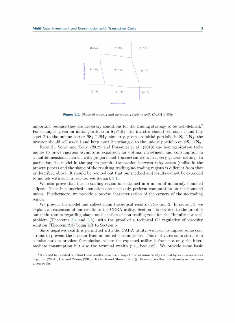
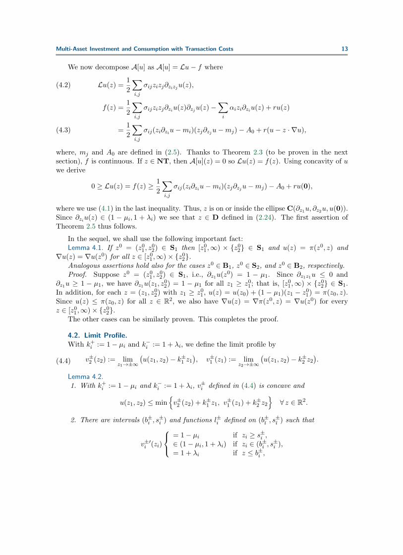
The main contribution of this paper is to provide a thorough characterization of theoptimal investment strategy for a risk-averse investor who can access multiple correlated riskyassets as well as a riskfree asset. We focus on the CARA utility case, and an extension tothe CRRA utility case is explained later. To illustrate our results, we take as an example thescenario of two risky assets. We will show that the shape of trading and no-trading regionsmust be as in Figure 1, where “Si”, “Bi”, and “Ni” represent selling, buying, and no tradingin asset i, respectively. The no-trading region N1 ∩ N2 locates in the center, surroundedby eight trading regions. Moreover, each intersection ∂S1 ∩ ∂S2, ∂S1 ∩ ∂B2, ∂B1 ∩ ∂S2, and∂B1 ∩ ∂B2 is a singleton. In addition, we show that the boundary of each of corner regionsS1 ∩ S2, S1 ∩B2, B1 ∩B2, and B1 ∩ S2 consists of one vertical and one horizontal half line,whereas the boundary of each of S1 ∩ N2, N1 ∩ S2, B1 ∩ N2, and N1 ∩ B2 consists of twoparallel either vertical or horizontal half lines and a curve in between connecting the end pointsof the two half lines. These characterizations on the shapes of trading regions are extremely

1There do exist many papers working on perturbation analysis or numerical solutions for the multiple risky-asset case, e.g. Law et al. (2009), Bichuch and Shreve (2011), Muthuraman and Kumar (2006), Dai and Zhong(2010).

Multi-Asset Investment and Consumption with Transaction Costs 3

Amount in Asset 1

Am

ount

inA

sset

2

S1 ∩ S2

S1 ∩N2

S1 ∩B2B1 ∩B2

B1 ∩N2

B1 ∩ S2 N1 ∩ S2

N1 ∩N2

N1 ∩B2

Figure 1.1. Shape of trading and no-trading regions with CARA utility

important because they are necessary conditions for the trading strategy to be well-defined.2

For example, given an initial portfolio in S1 ∩ B2, the investor should sell asset 1 and buyasset 2 to the unique corner ∂S1 ∩ ∂B2; similarly, given an initial portfolio in S1 ∩ N2, theinvestor should sell asset 1 and keep asset 2 unchanged to the unique portfolio on ∂S1 ∩N2.

Recently, Soner and Touzi (2012) and Possamaı et al. (2013) use homogenization tech-niques to prove rigorous asymptotic expansion for optimal investment and consumption ina multidimensional market with proportional transaction costs in a very general setting. Inparticular, the model in the papers permits transaction between risky assets (unlike in thepresent paper) and the shape of the resulting trading/no-trading regions is different from thatas described above. It should be pointed out that our method and results cannot be extendedto models with such a feature; see Remark 3.1.

We also prove that the no-trading region is contained in a union of uniformly boundedellipses. Thus in numerical simulation one need only perform computation on the boundedunion. Furthermore, we provide a precise characterization of the corners of the no-tradingregion.

We present the model and collect main theoretical results in Section 2. In section 3, weexplain an extension of our results to the CRRA utility. Section 4 is devoted to the proof ofour main results regarding shape and location of non-trading zone for the “infinite horizon”problem (Theorems 2.4 and 2.5), with the proof of a technical C1 regularity of viscositysolution (Theorem 2.3) being left to Section 5.

Since negative wealth is permitted with the CARA utility, we need to impose some con-straint to prevent the investor from unlimited consumptions. This motivates us to start froma finite horizon problem formulation, where the expected utility is from not only the inter-mediate consumption but also the terminal wealth (i.e., bequest). We provide some basic

2It should be pointed out that these results have been conjectured or numerically verified by some researchers[e.g. Liu (2004), Dai and Zhong (2010), Bichuch and Shreve (2011)]. However no theoretical analysis has beengiven so far.


properties of the value function associated with the finite horizon problem; in particular, welet the finite horizon T → ∞ to obtain the “infinite horizon” problem addressed in this paper.These results are presented as preliminaries in Section 2 and their proofs are placed in theAppendix.

2. Problem Formulation and Main Results. Consider a portfolio consisting of one risk-free asset (bank account) and n risky assets whose unit share prices are stochastic process(S0

t , S1t , · · · , Snt ) described by the stochastic differential equations

dS0t

S0t

= rdt,dSitSit

= αidt+n∑j=1

aijdWjt for i = 1, · · · , n,

where W 1t , · · · ,Wn

t t≥0 is a standard n-dimensional Wiener process, r > 0 is the constantbank rate, αi is the constant expected return rates of the i-th risky asset, and (aij)n×nis a constant positive definite matrix. We consider optimal strategies of investment andconsumption subject to transaction cost which are proportional to the amount of transactions.

2.1. Investment and Consumption. We introduce a non-negative parameter κ whereκ = 0 corresponds to the no-consumption case. Suppose the terminal time is T and currenttime is t < T . For s ∈ [t, T ), we denote by κcsds the consumption, deducted from the bankaccount, during time interval [s, s+ ds). Here we assume that κ has the same unit as r, being1/year, and that cs has the unit of dollars.

3 We denote by dLis the transfer of money from thebank account to the i-th risky assets during [s, s+ ds), which incurs purchasing costs λidL

is.

Similarly, we denote by dM is the money transferred from the i-th risky asset to the bank

account during [s, s + ds), which incurs selling costs µidMis. Here λi ≥ 0 and µi ∈ [0, 1) are

the constant proportions of transaction costs for purchasing and selling the i-th risky asset,respectively.

Let xs and ys = (y1s , · · · , yns ) be dollar values at time s ∈ [t, T ] invested in the bankaccount and risky assets, respectively. Their evolutions are described by

dxs = (rxs − κcs)ds−∑i

(1 + λi)dLis +

∑i

(1− µi)dMis,

dyis = yis(αids+∑j

aijdWjs ) + dLis − dM i

s, i = 1, · · · , n.(2.1)

For simplicity, we define an admissible (investment-consumption) strategy as S = (C,L,M)where C = css∈[t,T ], L = L1

s, · · · , Lns s∈[t,T ], and M = M1s , · · · ,Mn

s s∈[t,T ] are adaptedprocesses satisfying

dLis ≥ 0, dM is ≥ 0,(2.2)

and xs, yst≤s≤T is the solution of (2.1) subject to constant initial conditions. We denote byAt all the admissible strategies.

3The parameters κ and K in (2.3) below are both used as the weight between consumption and terminalwealth. However K is dimensionless while κ has the same unit as r. It should be pointed out that the conditionr < 1 in Chen et al. (2012) indeed means r < κ.


2.2. The Merton’s Problem. Given concave utilities U(x, y) and V (c) for the terminalportfolio and consumption respectively, a constant discount factor β > 0, and positive dimen-sionless constant weight K, we consider the measure of quality of an investment-consumptionstrategy S defined by

J(S, t) := KU(xT , yT )e−β(T−t) +

∫ T

tV (cs)e

−β(s−t)κds,(2.3)

where xs, yss∈[t,T ] is the solution of (2.1) with given strategy S ∈ At. The Merton’s problemis to maximize the expected utility:

Φ(x, y, t) = supS∈At

Ex,yt [J(S, t)] ∀x ∈ R, y ∈ Rn, t ≤ T,

where Ex,yt is the expectation under the condition (xt, yt) = (x, y). In this paper, we mainlyconsider the exponential utility

V (c) := −e−γc, U(x, y) := V (x+ ℓ(y)),

where ℓ(y) is the liquidation value of the holdings in the risky assets:

ℓ(y) =∑i

ℓi(yi), ℓi(yi) =

(1− µi)yi if yi ≥ 0,(1 + λi)yi if yi < 0.

(2.4)

Notice that ℓi(·) is a concave function and

ℓi(yi) = min1−µi≤k≤1+λi

kyi = min(1− µi)yi, (1 + λ)yi ∀ yi ∈ R.

For later use, we define

σij :=∑k

aikajk

and

mj :=∑i

σji(αi − r) ∀ j, A0 :=1

2

∑i,j

miσijmj ,(2.5)

where (σij)n×n is the inverse matrix of (σij)n×n. Here m := (m1, · · · ,mn) is the optimalinvestment strategy for the Merton’s problem without transaction costs, being the solution ofthe linear system ∑

j

σijmj = αi − r ∀ i = 1, · · · , n.


2.3. Preliminary Results. With the exponential utility, we have the following:Theorem 2.1. There exists a function ψ defined on Rn × [0,∞) such that

Φ(x, y, t) = −e−γξ(τ)x+(r−β)b(τ)+Z(τ) lnK−ln ξ(τ)−ψ(z,τ),(2.6)

where τ = T − t, z = γξ(τ)y, and ξ, Z, b are defined by

ξ(τ) =rerτ

r + κerτ − κ, Z(τ) = ξ(τ)e−rτ , b(τ) =

κ(erτ − 1− rτ) + r2τ

r(r + κerτ − κ),(2.7)

i.e., unique solutions of the following

ξ′ = (r − κξ)ξon [0,∞), ξ(0) = 1;(2.8)

Z ′ = −κξZon [0,∞), Z(0) = 1;(2.9)

b′ = −κξb+ 1on [0,∞), b(0) = 0.(2.10)

In addition,(1) for each τ ≥ 0, ψ(·, τ) is Lipschitz continuous:

ℓ(z − z) ≤ ψ(z, τ)− ψ(z, τ) ≤ −ℓ(z − z) ∀ z, z ∈ Rn;(2.11)

(2) for A0 defined in (2.5),

ℓ(z) ≤ ψ(z, τ) ≤ ℓ(z) +A0b(τ) ∀ z ∈ Rn, τ ≥ 0;(2.12)

(3) for each τ ≥ 0, ψ(·, τ) is concave;(4) ψ is a viscosity solution of min

∂τψ −Aτ [ψ], B(∇ψ)

= 0 in Rn × (0,∞),

ψ(·, 0) = ℓ(z) on Rn × 0,(2.13)

where Aτ and B are defined by

Aτ [ψ] :=1

2

∑i,j

σijzizj(∂zizjψ−∂ziψ∂zjψ) +∑i

(αi−r)zi∂ziψ + κξ(τ) [z · ∇ψ − ψ],(2.14)

B(p) := mini

min1 + λi − pi,−1 + µi + pi ∀ p = (p1, · · · , pn) ∈ Rn.(2.15)

We regard the infinite horizon problem as the limit of finite horizon problem under ap-propriate scales, as the finite horizon T → ∞. For this, we have the following:

Theorem 2.2.Suppose κ > 0. Then there exist a function u and a constant M such that

|∂τψ(z, τ)|+ |ψ(z, τ)− u(z)| ≤M(1 + rτ)e−rτ ∀ τ > 0, z ∈ Rn.(2.16)

In addition, u is a Lipschitz continuous concave viscosity solution of the following equation

min−A[u], B(∇u) = 0, 0 ≤ u− ℓ ≤ A0

rin Rn(2.17)


where ℓ(z), A0, and B are defined in (2.4), (2.5), and (2.15) respectively, and

A[u] :=1

2

∑i,j

σijzizj(∂zizju− ∂ziu∂zju) +∑i

αizi∂ziu− ru.(2.18)

The estimate (2.16) implies that ψ and ∂τψ converge at an exponential rate governed bythe interest rate r > 0, instead of the discount factor β. If r goes to 0, the analytic infinitehorizon optimal strategy in the absence of transaction costs indicates that the dollar valuesinvested in risky assets and consumption tend to infinity [see, e.g., Merton (1969) and Chenet al. (2012)]. 4

The proof of the above two theorems is given in the Appendix.

2.4. Main Results. We are mainly interested in the infinite horizon problem. Recall thatτ = T − t and z = γξ(τ)y. Hence, setting ΦT (x, y) = Φ(x, y, 0) where Φ is the solution of thefinite T -horizon problem, we have, when κ > 0,

Φ∞(x, y) := limT→∞

ΦT (x, y) = − limT→∞

e(r−β)b(T )−γξ(T )x+z(T ) lnK−ln ξ(T )−ψ(γξ(T )y,T )

= −e(r−β)b(∞)−γξ(∞)x+Z(∞) lnK−ln ξ(∞)−u(γξ(∞)y)

= −κre(r−β)/r−γrx/κ−u(γry/κ).

Hence, the solution u to the equation (2.17) can be formally regarded as the value functionassociated with the infinite horizon utility maximization problem:

Φ∞(x, y) = supS∈A∞

Ex,y0

[∫ ∞

0V (cs)e

−βsds

]where A∞ is certain admissible strategy. Note that without any restriction on A∞, theoptimal strategy is cs ≡ ∞. Hence, if one considers directly the infinite horizon problem,some technical conditions should be given [see, e.g., Liu (2004)]. We instead regard theinfinite horizon problem as the limit, as T → ∞, of the finite T -horizon problem with theaddition of a bequest utility which prevents unlimited consumption.

For solution u of the “infinite horizon” problem (2.17), we have the following regularityresult that plays a critical role in the analysis of the shape and location of the trading andno-trading regions:

Theorem 2.3. Let u be the solution of (2.17). Then zi∂ziu ∈ C(Rn) for each i = 1, · · · , n;consequently, u ∈ C1(Ω) where Ω = (z1, · · · , zn) ∈ Rn |

∏i zi = 0.

The shape of the trading and no-trading regions is characterized by the following:Theorem 2.4. Assume that 5 n = 2 and for i = 1, 2 define

Bi := z | ∂ziu(z) = 1 + λi,Si := z | ∂ziu(z) = 1− µi,Ni := z | 1− µi < ∂ziu(z) < 1 + λi,

4It should be admitted that the model with the CARA utility discussed here is less plausible than the onewith the CRRA utility.

5Here we consider only the two dimensional case. We expect that analogous results remain true for thehigher dimensional case.


and denote SS = S1 ∩ S2, SN = S1 ∩ N2, SB = S1 ∩ B2, NS = N1 ∩ S2, NT = N1 ∩N2, NB = N1 ∩B2, BS = B1 ∩ S2, BN = B1 ∩N2, and BB = B1 ∩B2. Then

(1) For i = 1, 2, there are bounded functions l±i (·) (defined on Rn−1 = R)such that

Bi = (z1, z2) | zı ∈ R, zi ≤ l−i (zı),Si = (z1, z2) | zı ∈ R, zi ≥ l+i (zı),Ni = (z1, z2) | zı ∈ R, l−i (zı) < zi < l+i (zı)

(2.19)

where ı = 1, 2 \ i, i.e., ı = 2 if i = 1 and ı = 1 if i = 2.(2) Each intersection ∂S1 ∩ ∂S2, ∂S1 ∩ ∂B2, ∂B1 ∩ ∂S2, and ∂B1 ∩ ∂B2 is a singleton, so

the four boundaries ∂S1, ∂B1, ∂S2, ∂B2 divide the plane into nine regions, with open regionNT in the center surrounded in clockwise order by closed regions SS, SN, SB, NB, BB,BN, BS, and NS.

(3) The boundary of each of corner regions SS, SB, BB, and BS consists of one verticaland one horizontal half line, whereas the boundary of each of SN, NS, BN, and NB consistsof two parallel either vertical or horizontal half lines and a curve in between connecting theend points of the two half lines; c.f. Figure 1.

We remark when n ≥ 3, ı = 1, · · · , n\i, so li(zı) is indeed a function of n−1 variables.The theorem implies the following: There are intervals [b±i , s

±i ] such that

SS = [s+1 ,∞)× [s+2 ,∞),

SN = (z1, z2) | z2 ∈ (b+2 , s+2 ), z1 ≥ l+1 (z2),

SB = [s−1 ,∞)× (−∞, b+2 ],

NB = (z1, z2) | z1 ∈ (b−1 , s−1 ), z2 ≤ l−2 (z1),

BB = (−∞, b−1 ]× (−∞, b−2 ],

BN = (z1, z2) | z2 ∈ (b−2 , s−2 ), z1 ≤ l−1 (z2),

BS = (−∞, b+1 ]× [s−2 ,∞),

NS = (z1, z2) | z1 ∈ (b+1 , s+1 ), z2 ≥ l+2 (z1).

The no-trading region NT is bounded by four curves: Γ2+ from the right, Γ2− from the left,Γ1+ from the top, and Γ1− from the bottom where

Γ2± := (l±1 (z2), z2) | z2 ∈ (b±2 , s±2 ), Γ1± := (z1, l±2 (z1)) | z1 ∈ (b±1 , s

±1 ).

These four curves connect each other only at their tips:l±i (b

±ı ) = limzıb±ı

l±i (zı), l±i (s±ı ) = limzıs±ı

l±i (zı),

(b+1 , l+2 (b

+1 )) = (l−1 (s

−2 ), s

−2 ), (l+1 (s

+2 ), s

+2 ) = (s+1 , l

+2 (s1)),

(l−1 (b−2 ), b

−2 ) = (b−1 , l

−2 (b

−1 )), (s−1 , l

−2 (s

−1 )) = (l+1 (b

+2 ), b

+2 ).

(2.20)

Each function l±i is constant outside (b±ı , s±ı ):

l±i (zı) = l±i (b±ı ) ∀ zı ≤ b±ı , l±i (zı) = l±i (s

±ı ) ∀ zı ≥ s±ı .(2.21)


As emphasized in the introduction, Theorem 2.4 is very much needed for the tradingstrategy to be well-defined. It is well-known that except at the initial time, transactionsoccur at the boundary of the no-trading region. When the initial portfolio falls outside theno-trading region, the shape of the trading regions stated in the theorem implies a uniquetrading strategy to move the portfolio to the boundary of the no-trading region. However,at this stage we cannot prove the smoothness of the curves l±i ,

6 so we are unable to proverigorously the optimal controlled portfolio process as a reflected diffusion as in Davis andNorman (1990) and Shreve and Soner (1994).

We can now state our main result regarding the location of no trading region:

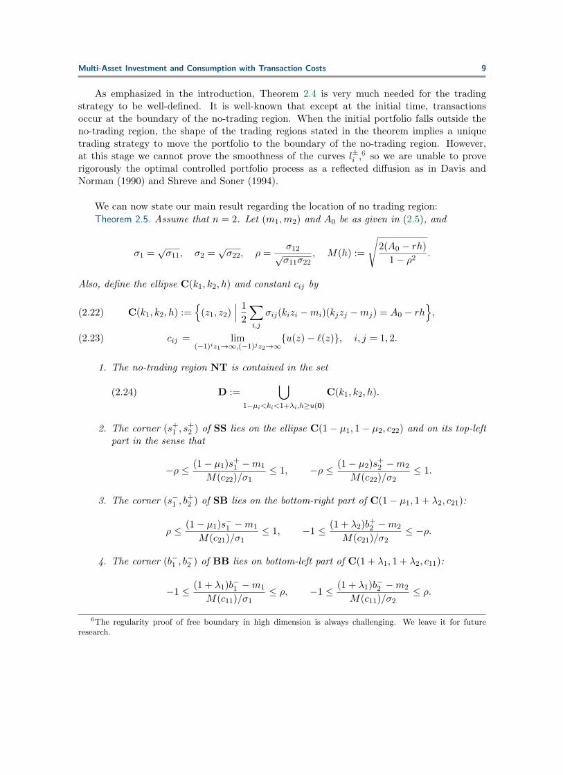
Theorem 2.5. Assume that n = 2. Let (m1,m2) and A0 be as given in (2.5), and

σ1 =√σ11, σ2 =

√σ22, ρ =

σ12√σ11σ22

, M(h) :=

√2(A0 − rh)

1− ρ2.

Also, define the ellipse C(k1, k2, h) and constant cij by

C(k1, k2, h) :=(z1, z2)

∣∣∣ 12

∑i,j

σij(kizi −mi)(kjzj −mj) = A0 − rh,(2.22)

cij = lim(−1)iz1→∞,(−1)jz2→∞

u(z)− ℓ(z), i, j = 1, 2.(2.23)

1. The no-trading region NT is contained in the set

D :=∪

1−µi<ki<1+λi,h≥u(0)

C(k1, k2, h).(2.24)

2. The corner (s+1 , s+2 ) of SS lies on the ellipse C(1− µ1, 1− µ2, c22) and on its top-left

part in the sense that

−ρ ≤ (1− µ1)s+1 −m1

M(c22)/σ1≤ 1, −ρ ≤ (1− µ2)s

+2 −m2

M(c22)/σ2≤ 1.

3. The corner (s−1 , b+2 ) of SB lies on the bottom-right part of C(1− µ1, 1 + λ2, c21):

ρ ≤ (1− µ1)s−1 −m1

M(c21)/σ1≤ 1, −1 ≤ (1 + λ2)b

+2 −m2

M(c21)/σ2≤ −ρ.

4. The corner (b−1 , b−2 ) of BB lies on bottom-left part of C(1 + λ1, 1 + λ2, c11):

−1 ≤ (1 + λ1)b−1 −m1

M(c11)/σ1≤ ρ, −1 ≤ (1 + λ1)b

−2 −m2

M(c11)/σ2≤ ρ.

6The regularity proof of free boundary in high dimension is always challenging. We leave it for futureresearch.


5. The corner (b+1 , s−2 ) of BS lies on top-left of C(1 + λ1, 1− µ2, c12):

−1 ≤ (1 + λ1)b+1 −m1

M(c12)/σ1≤ −ρ, ρ ≤ (1− µ2)s

−2 −m2

M(c12)/σ2≤ 1.

We remark that

0 ≤ u(0) ≤ cij ≤A0

r

since 0 ≤ u(z)− ℓ(z) ≤ A0/r and u(z)− ℓ(z) is an increasing concave function in each radialdirection.

The theorem shows that the no-trading region is contained in a union of uniformly boundedellipses. Moreover, the location of the corners of the no-trading region is estimated. Hence wecan restrict attention to a bounded domain to study the problem. In particular, this allowsus to do computations in a bounded domain.

The proof of Theorems 2.4 and 2.5 will be given in Section 4 and the proof of Theorem2.3 in Section 5.

3. Extension to the CRRA Utility. Now let us examine the case with the CRRA utility,namely,

V (c) =1

γcγ , γ < 1, γ = 0,

for which we require that the liquidated wealth be non-negative:

x+∑i

ℓi(yi) ≥ 0.

Note that we can directly consider the infinite horizon problem for the CRRA utility and theabove solvency constraint. Let Φ (x, y1, y2) be the associated value function which satisfies(cf. Dai and Zhong (2010))

(3.1) min

−LΦ,min

i[(1 + λi) ∂xΦ− ∂yiΦ] ,min

i[− (1− µi) ∂xΦ+ ∂yiΦ]

= 0,

in x+∑

i ℓi(yi) > 0, where L is as given in (A.6).For illustration, we still consider the case of two risky assets. The homogeneity of the

utility function allows us to make the following transformation:

zi =yi

x+ y1 + y2, i = 1, 2,

φ (z1, z2) ≡ Φ(1− z1 − z2, z1, z2) =1

(x+ y1 + y2)γΦ(x, y1, y2) .

Then (3.1) reduces to

min

−Aφ,min

i

[λiγφ−

∑k

(δik + λizk) ∂zkφ

],min

i

[µiγφ−

∑k

(−δik + µizk) ∂zkφ

]= 0


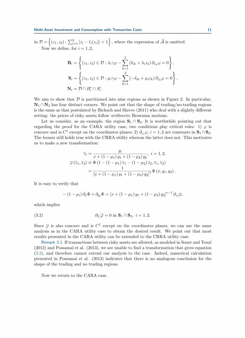
in D =(z1, z2) :

∑2i=1 [zi − ℓi(zi)] < 1

, where the expression of A is omitted.

Now we define, for i = 1, 2,

Bi =

(z1, z2) ∈ D : λiγφ−

2∑k=1

(δik + λizk) ∂zkφ = 0

,

Si =

(z1, z2) ∈ D : µiγφ−

2∑k=1

(−δik + µizk) ∂zkφ = 0

,

Ni = D ∩Bci ∩ Sci .

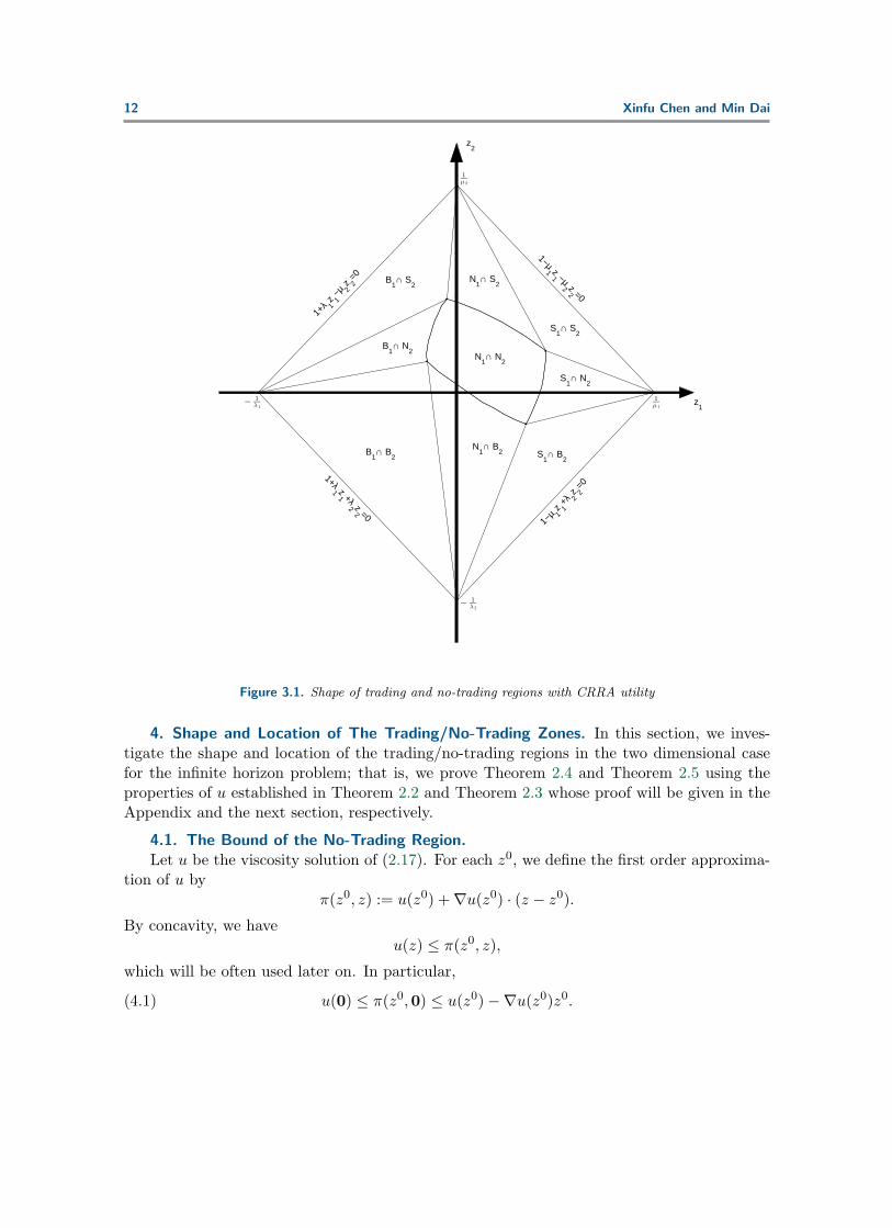
We aim to show that D is partitioned into nine regions as shown in Figure 2. In particular,N1 ∩N2 has four distinct corners. We point out that the shape of trading/no-trading regionsis the same as that postulated by Bichuch and Shreve (2011) who deal with a slightly differentsetting: the prices of risky assets follow arithmetic Brownian motions.

Let us consider, as an example, the region S1 ∩ S2. It is worthwhile pointing out thatregarding the proof for the CARA utility case, two conditions play critical roles: 1) φ isconcave and is C1 except on the coordinates planes; 2) ∂ziφ, i = 1, 2 are constants in S1 ∩S2.The former still holds true with the CRRA utility whereas the latter does not. This motivatesus to make a new transformation:

zi =yi

x+ (1− µ1) y1 + (1− µ2) y2, i = 1, 2,

φ (z1, z2) ≡ Φ(1− (1− µ1) z1 − (1− µ2) z2, z1, z2)

=1

[x+ (1− µ1) y1 + (1− µ2) y2]γΦ(x, y1, y2) .

It is easy to verify that

− (1− µi) ∂xΦ+ ∂yiΦ = [x+ (1− µ1) y1 + (1− µ2) y2]γ−1 ∂ziφ,

which implies

(3.2) ∂ziφ = 0 in S1 ∩ S2, i = 1, 2.

Since φ is also concave and is C1 except on the coordinates planes, we can use the sameanalysis as in the CARA utility case to obtain the desired result. We point out that mostresults presented in the CARA utility can be extended to the CRRA utility case.

Remark 3.1. If transactions between risky assets are allowed, as modeled in Soner and Touzi(2012) and Possamaı et al. (2013), we are unable to find a transformation that gives equation(3.2), and therefore cannot extend our analysis to the case. Indeed, numerical calculationpresented in Possamaı et al. (2013) indicates that there is no analogous conclusion for theshape of the trading and no trading regions.

Now we return to the CARA case.


1+λ 1

z 1−µ 2

z 2=0

1−µ1 z

1 −µ2 z

2 =0

1+λ1 z

1 +λ2 z

2 =01−

µ 1z 1

+λ 2z 2

=0

z2

z1

B1∩ S

2

B1∩ N

2

B1∩ B

2 S1∩ B

2

N1∩ B

2

S1∩ N

2

S1∩ S

2

N1∩ S

2

N1∩ N

2

−

1

λ 2

−

1

λ 1

1

µ2

1

µ1

Figure 3.1. Shape of trading and no-trading regions with CRRA utility

4. Shape and Location of The Trading/No-Trading Zones. In this section, we inves-tigate the shape and location of the trading/no-trading regions in the two dimensional casefor the infinite horizon problem; that is, we prove Theorem 2.4 and Theorem 2.5 using theproperties of u established in Theorem 2.2 and Theorem 2.3 whose proof will be given in theAppendix and the next section, respectively.

4.1. The Bound of the No-Trading Region.Let u be the viscosity solution of (2.17). For each z0, we define the first order approxima-

tion of u byπ(z0, z) := u(z0) +∇u(z0) · (z − z0).

By concavity, we haveu(z) ≤ π(z0, z),

which will be often used later on. In particular,

u(0) ≤ π(z0,0) ≤ u(z0)−∇u(z0)z0.(4.1)


We now decompose A[u] as A[u] = Lu− f where

Lu(z) = 1

2

∑i,j

σijzizj∂zizju(z),(4.2)

f(z) =1

2

∑i,j

σijzizj∂ziu(z)∂zju(z)−∑i

αizi∂ziu(z) + ru(z)

=1

2

∑i,j

σij(zi∂ziu−mi)(zj∂zju−mj)−A0 + r(u− z · ∇u),(4.3)

where, mj and A0 are defined in (2.5). Thanks to Theorem 2.3 (to be proven in the nextsection), f is continuous. If z ∈ NT, then A[u](z) = 0 so Lu(z) = f(z). Using concavity of uwe derive

0 ≥ Lu(z) = f(z) ≥ 1

2

∑i,j

σij(zi∂ziu−mi)(zj∂zju−mj)−A0 + ru(0),

where we use (4.1) in the last inequality. Thus, z is on or inside the ellipse C(∂z1u, ∂z2u, u(0)).Since ∂ziu(z) ∈ (1 − µi, 1 + λi) we see that z ∈ D defined in (2.24). The first assertion ofTheorem 2.5 thus follows.

In the sequel, we shall use the following important fact:Lemma 4.1. If z0 = (z01 , z

02) ∈ S1 then [z01 ,∞) × z02 ∈ S1 and u(z) = π(z0, z) and

∇u(z) = ∇u(z0) for all z ∈ [z01 ,∞)× z02.Analogous assertions hold also for the cases z0 ∈ B1, z

0 ∈ S2, and z0 ∈ B2, respectively.

Proof. Suppose z0 = (z01 , z02) ∈ S1, i.e., ∂z1u(z

0) = 1 − µ1. Since ∂z1z1u ≤ 0 and∂z1u ≥ 1 − µ1, we have ∂z1u(z1, z

02) = 1 − µ1 for all z1 ≥ z01 ; that is, [z01 ,∞) × z02 ∈ S1.

In addition, for each z = (z1, z02) with z1 ≥ z01 , u(z) = u(z0) + (1 − µ1)(z1 − z01) = π(z0, z).

Since u(z) ≤ π(z0, z) for all z ∈ R2, we also have ∇u(z) = ∇π(z0, z) = ∇u(z0) for everyz ∈ [z01 ,∞)× z02.

The other cases can be similarly proven. This completes the proof.

4.2. Limit Profile.With k+i := 1− µi and k

−i := 1 + λi, we define the limit profile by

v±2 (z2) := limz1→±∞

(u(z1, z2)− k±1 z1

), v±1 (z1) := lim

z2→±∞

(u(z1, z2)− k±2 z2

).(4.4)

Lemma 4.2.1. With k+i := 1− µi and k

−i := 1 + λi, v

±i defined in (4.4) is concave and

u(z1, z2) ≤ minv±2 (z2) + k±1 z1, v

±1 (z1) + k±2 z2

∀ z ∈ R2.

2. There are intervals (b±i , s±i ) and functions l±i defined on (b±ı , s

±ı ) such that

v±i′(zi)

= 1− µi if zi ≥ s±i ,∈ (1− µi, 1 + λi) if zi ∈ (b±i , s

±i ),

= 1 + λi if z ≤ b±i ,


u(z1, z2) =

v+2 (z2) + (1− µ1)z1 if z1 ≥ l+1 (z2), z2 ∈ (b+2 , s+2 ),

v−2 (z2) + (1 + λ1)z1 if z1 ≤ l−1 (z2), z2 ∈ (b−2 , s−2 ),

v+1 (z1) + (1− µ2)z2 if z2 ≥ l+2 (z1), z1 ∈ (b+1 , s+1 ),

v−1 (z1) + (1 + λ2)z2 if z2 ≤ l−2 (z1), z1 ∈ (b−1 , s−1 ),

∂z1u(z1, z2) > 1− µ1 if z1 < l+1 (z2), z2 ∈ (b+2 , s+2 ),

∂z1u(z1, z2) < 1 + λ1 if z1 > l−1 (z2), z2 ∈ (b−2 , s−2 ),

∂z2u(z1, z2) > 1− µ2 if z2 < l+2 (z1), z1 ∈ (b+1 , s+1 ),

∂z2u(z1, z2) < 1 + λ2 if z2 > l−2 (z1), z1 ∈ (b−1 , s−1 ).

3. Define

l±i (s±ı ) = lim

zıs±ı

l±i (zı), l±i∗(s±ı ) = lim

zıs±ı

l±i (zı),

l±i (b±ı ) = lim

zıbı

l±i (zı), l±i∗(b±ı ) = lim

zıbıl±i (zı).

Then

[l+1 (s+2 ), l

+1∗(s

+2 )]× s+2 ∪ s+1 × [l+2 (s

+1 ), l

+2∗(s

+1 )] ⊂ ∂NT ∩ SS,

[l+1 (b+2 ), l

+1∗(b

+2 )]× b+2 ∪ s−1 × [l−2 (s

−1 ), l

−2∗(s

−1 )] ⊂ ∂NT ∩ SB,

[l+1 (s−2 ), l

+1∗(s

−2 )]× s−2 ∪ b+1 × [l+2 (b

+1 ), l

+2∗(b

+1 )] ⊂ ∂NT ∩BS,

[l+1 (b−2 ), l

+1∗(b

−2 )]× b−2 ∪ b−1 × [l+2 (b

−1 ), l

−2∗(s

−1 )] ⊂ ∂NT ∩BB.

Proof. By symmetry, we need only consider the function v := v+2 .(1) Note that u(z1, z2) − (1 − µ1)z1 is a concave function, ∂z1 [u(z1, z2) − (1 − µ1)z1] =

∂z1u−(1−µ1) ≥ 0, and 0 ≤ u(z)−ℓ(z) ≤ A0/r. Hence, v(z2) := limz1→∞[u(z1, z2)−(1−µ1)z1]exists, v is concave, and v(z2) ≥ u(z1, z2)− (1− µ1)z1.

(2) Let z2 ∈ R be a generic point such that 1−µ2 < v′(z2) < 1+ λ2. Since ∂z2u(z1, z2) →v′(z2) as z1 → ∞, ∂z2u(z1, z2) ∈ (1− µ2, 1 + λ2) for all z1 ≫ 1. As NT is bounded, we musthave ∂z1u(z1, z2) = 1 − µ1 for all z1 ≫ 1. In addition, since ∂z1u → 1 + λ1 as z1 → −∞, wecan define

l(z2) := minz1 ∈ R | ∂z1u(z1, z2) = 1− µ1.

Since u(·, z2) is concave, we must have

∂z1u(z1, z2) < 1− µ1 ∀ z1 < l(z2), ∂z1u(z1, z2) = 1− µ1 ∀ z1 ≥ l(z2).

Denote z0 := (l(z2), z2). Then by Lemma 4.1, u(z) = π(z0, z) = v(z02) + (1 − µ1)z1and ∇u(z) = ∇u(z0) for each z ∈ [l(z2),∞) × z2. Consequently, ∂z2u(z1, z2) = v′(z2) ∈(1 − µ2, 1 + λ2) for all z1 ∈ [l(z2),∞). Thus, for small positive ε, B(∇u(z)) > 0 on [l(z2) −


ε, l(z2)) × z2. Hence, [l(z2) − ε, l(z2)) × z2 ∈ NT and (l(z2), z2) ∈ ∂NT. Since NT isbounded and v is concave, there exist bounded b and s such that

v′ = 1 + λ2 on (−∞, b], 1 + λ2 > v′ > 1− µ2 on (b, s), v′ = 1− µ2 on [s,∞).

(3) Now we define l(s) = limz2s l(z2), l∗(s) = limz2s l(z2), and z∗ = (l(s), s). Bycontinuity, we have ∂z1u(l(s), s) = 1 − µ1. This implies that ∇u(z) = (1 − µ1, v

′(s)) =(1− µ1, 1− µ2) for all z ∈ [l(s),∞)× s. Hence, [l(s),∞)× s ∈ SS.

Note that for each z2 < s and z1 ∈ [l(s),∞), we have

u(z1, s)− u(z1, z2) = v(s)− v(z2)−∫ ∞

z1

[∂z1u(ξ, s)− ∂z1u(ξ, z2)]dξ

=

∫ s

z2

v′(y)dy +

∫ ∞

z1

[∂z1u(ξ, z2)− (1− µ1)]dξ > (1− µ2)(s− z2).

It follows by concavity that ∂z2u(z1, z2) > 1− µ2. Hence,

∂z2u > 1− µ2 on [l(s),∞)× (−∞, s).(4.5)

It then follows by the definition of l(s) and l∗(s) that [l(s), l∗(s)]× s ⊂ ∂NT.Similarly we can work on the other functions v±i to complete the proof of Lemma 4.2.

4.3. The Intersection of ∂NT with B1 ∩B2, S1 ∩ S2 and Bi ∩ Sj.In this subsection we prove the following:Lemma 4.3. Let cij and C(k1, k2, h) be defined as in (2.23) and (2.22).1. The set ∂NT ∩ SS is a single point on top-right of the ellipse C(1 − µ1, 1 − µ2, c22).

In addition, if (z01 , z02) ∈ SS, then [z01 ,∞)× [z02 ,∞) ⊂ SS.

2. The set ∂NT ∩ SB is a single point on bottom-right of C(1 − µ1, 1 + λ2, c21). If(z01 , z

02) ∈ SB, then [z01 ,∞)× (−∞, z02 ] ⊂ SB.

3. The set ∂NT∩BB is a single point on bottom-left of C(1+λ1, 1+λ2, c11). If (z01 , z

02) ∈

BB, then (−∞, z01 ]× (−∞, z02 ] ⊂ BB.4. The set ∂NT∩BS is a single point on top-left of C(1+λ1, 1−µ2, c12). If (z01 , z02) ∈ BS,

then (−∞, z01 ]× [z02 ,∞) ⊂ BS.Proof. (i) Suppose z0 = (z01 , z

02) ∈ S1 ∩ S2.

First we show that [z01 ,∞) × [z02 ,∞) ⊂ SS. Indeed by Lemma 4.1, u(z) = π(z0, z) on([z01 ,∞)×z02)∪ (z10× [z02 ,∞)). This implies that u(·) ≥ π(z0, ·) on [z01 ,∞)× [z02 ,∞) sinceπ(z0, ·) is linear and u(·) is concave. On the other hand, we have u(z) ≤ π(z0, z) on R2. Thuswe must have u(z) = π(z0, z) and ∇u(z) = ∇u(z0) = (1−µ1, 1−µ2) so [z01 ,∞)×[z02 ,∞) ⊂ SS.In addition, on [z01 ,∞)× [z02 ,∞),

u(z) = u(z0) + (1− µ1)(z1 − z01) + (1− µ2)(z2 − z02) = c22 + z · ∇u(z0).

Next since −A[u] = f(z)−Lu ≥ 0 on R2, using the linearity of u on [z01 ,∞)× [z02 ,∞) weobtain

0 = lims0

Lu(z0 + se1 + se2) ≤ lims0

f(z0 + se1 + se2) = f(z0).


Using u = c22 + z · ∇u(z0) on [z01 ,∞)× [z02 ,∞) we find that f(z0) = f22(z0) ≥ 0 where

f22(z) :=1

2

∑i,j

σij(zi[1− µi]−mi)(zj [1− µj ]−mj)−A0 + rc22 ∀ z ∈ R2.

This analysis in particular implies that f22(z) ≥ 0 for every z ∈ SS.(ii) Next, suppose z0 ∈ ∂NT ∩ SS. Note that when z ∈ NT, we have 0 = −A[u](z) =

f(z)− Lu[z], i.e. f(z) = L[u](z) ≤ 0 (as u is concave). Hence,

f(z0) = limz∈NT,z→z0

f(z) = limz∈NT,z→z0

Lu(z) ≤ 0.

Thus, we must have f(z0) = 0, i.e., z0 ∈ C := C(1−µ1, 1−µ2, c22). Moreover, since f22(z) ≥ 0for every z ∈ [z01 ,∞) × [z02 ,∞) and f(z) < 0 for each z inside the ellipse C, we see that z0

lies on the top-right part of the ellipse C. Locating the highest and rightmost points of theellipse C, we then derive that

f22(z0) = 0, −ρ ≤ (1− µ1)z

01 −m1

M(c22)/σ1≤ 1, −ρ ≤ (1− µ2)z

02 −m2

M(c22)/σ2≤ 1.

(iii) Now we show that ∂NT ∩ SS is a singleton, by a contradiction argument. Supposez0 = (z01 , z

02) ∈ ∂NT∩SS, z0 = (z01 , z

02) ∈ ∂NT∩SS, and z0 = z0. Then both z0 and z0 lies on

the upper-right part of the ellipse C(1−µ1, 1−µ2, c22). Exchanging the roles of z0 and z0, wecan assume that z02 < z02 and z01 > z01 . Note that u(z) = π(z0, z) for all z ∈ [z01 ,∞)× (z02 ,∞)and u(z) = π(z0, z) for all z ∈ [z01 ,∞) ∩ [z02 ,∞). Hence, π(z0, z) = π(z0, z) for all z ∈ R2. Onthe other-hand, if u(z) = π(z0, z), then ∇u(z) = ∇π(z0, z) = ∇u(z0) so z ∈ SS. Therefore,

SS := z ∈ R2 | ∇u(z) = (1− µ1, 1− µ1) = z ∈ R2 | u(z) = π(z0, z).

Note that u is concave, π(z0, ·) is linear, and u(·) ≤ π(z0, ·) on Rn. We derive that SS is aconvex set. Consequently, it contains L, the line segment connecting z0 and z0.

Next for each s ∈ R, denote zs = (z01 , z02) + (s, s). For s < 0, zs ∈ SS since otherwise

it would imply [z01 + s,∞) × [z02 + s,∞) ∈ SS, contradicting z0 ∈ ∂NT. Hence, there existss∗ ≥ 0 such that z∗ = (z01 + s∗, z02 + s∗) ∈ ∂(SS). The point z∗ lies on or below L so is aninterior point of the ellipse C. There are two cases: (a) s∗ > 0, and (b) s∗ = 0.

Consider case (a) s∗ > 0. Then for each s ∈ [0, s∗), zs ∈ SS since SS is convex. Also∂z1u(z

s) > 1−µ1 since by Lemma 4.1, ∂z1u(zs) = 1−µ1 would imply that ∇u(zs) = ∇u(z) =

∇u(z0) where z is the intersection of L with the line z2 = z02 + s. Similarly, ∂z2u(zs) > 1−µ2.

for each s ∈ [0, s∗). Thus, zs ∈ NT for all s ∈ [0, s∗). This means that zs∗ ∈ ∂NT ∩ SS,

which is impossible since zs∗ ∈ C.

Consider case (b) s∗ = 0. First of all ∂z1u(z1, z02) > 1− µ1 for all z1 < z01 since otherwise

it would imply ∇u(z1, z02) = ∇u(z0) and thus [z1,∞)× [z02 ,∞) ∈ SS contradicting z0 ∈ ∂NT.Similarly, ∂z2u(z

01 , z2) > 1−µ2 for every z2 < z02 . Now for every small positive ε, consider the

closed setDε := [z01 − ε, z01 ]× [z02 − ε, z02 ] \ (z01 − ε/2, z01 ]× (z02 − ε/2, z02 ].

If z∗ = (z∗1 , z∗2) ∈ SS ∩ Dε we would have z∗1 < z01 and z∗2 < z02 so z0 is an interior point of

[z∗1 ,∞) × [z∗2 ,∞) ⊂ SS, a contradiction. Thus, SS ∩ Dε = ∅. Consequently, the closed sets


Dε ∩ S1 and Dε ∩ S2 are disjoint. Since Dε cannot be written as the union of two disjointclosed proper subsets, the set Dε \ (S1 ∪ S2) is non-empty. This means that Dε ∩ NT = ∅.Consequently, (z01 , z

02) ∈ ∂NT ∩ SS, but this is impossible since (z01 , z

02) does not lie on C.

Therefore ∂NT ∩ SS is a singleton.The proof for the singleness of ∂NT ∩ BS, ∂NT ∩ SB, and ∂NT ∩ BB is similar. This

completes the proof of the Lemma.

4.4. Completion of the Proof of Theorems 2.4, 2.5.By Lemmas 4.2 and 4.3, we see that the limits in (2.20) exist, and the limits satisfy the

matching condition stated in (2.20). We extend l±i from (b±ı , s±ı ) to R by (2.21).

By the definition of l+2 on (b+1 , s+1 ) we know that when z1 ∈ (b+1 , s

+1 ), ∂z2u(z1, z2) > 1−µ2

if and only if z2 < l+2 (z1). Also, in view of (4.5) and the matching (2.20), we derive that whenz1 ∈ [s+1 ,∞), ∂z2u(z1, z2) > 1−µ2 if and only if z2 < l+2 (s

+1 ) = l+2 (z1). Similarly, we can show

that when z1 ∈ (−∞, b+1 ], ∂z2u(z1, z2) < 1− µ2 if and only if z2 < l+2 (b+1 ) = l+2 (z1). Thus,

S2 := z | ∂z2u = 1− µ2 = (z1, z2) | z1 ∈ R, z2 ≥ l+2 (z1).

Similarly, we can show the other equations in (2.19). The rest assertions of Theorems 2.4 and2.5 thus follow from Lemmas 4.2 and 4.3. This completes the proof of Theorems 2.4 and 2.5.

5. C1 Regularity. In this section we prove Theorem 2.3; that is, we show that the viscositysolution u of the “infinite horizon” problem (2.17) is C1 except on the coordinates planes wherethe elliptic operator A is degenerate. The C1 continuity plays a critical role in the previoussection where a key step is to derive the continuity of f(·) defined in (4.3).

We begin with recalling the definition of a viscosity solution:Definition 5.1.A function u defined on Rn is called a viscosity solution of (2.17) if u is

continuous, u− ℓ ∈ L∞(Rn), and the following holds:1. If ζ is a C2 function in Bε(z

0) := z ∈ Rn | |z− z0| < ε for some z0 ∈ Rn and ε > 0,and that ζ(z)− u(z) ≥ 0 = ζ(z0)− u(z0) for every z ∈ Bε(z

0), then

min−A[ζ](z0), B(∇ζ(z0))

≤ 0.

2. If ζ is a C2 function in Bε(z0) := z ∈ Rn | |z− z0| < ε for some z0 ∈ Rn and ε > 0,and that ζ(z)− u(z) ≤ 0 = ζ(z0)− u(z0) for each z ∈ Bε(z

0), then

min−A[ζ](z0), B(∇ζ(z0))

≥ 0.

One can show that the viscosity solution of (2.17) is unique. Since the solution is the limitof ψ(·, τ) that is concave, we see that the viscosity solution of (2.17) is concave. We shall usethis fact to prove the C1 regularity of u.

For any function f defined on Rn, we define its super-differential by

∂f(z) = p ∈ Rn : f(z) ≤ f(z) + p · (z − z) ∀ z ∈ Rn.(5.1)

We shall use the following fact.Lemma 5.2.Suppose f is a concave function on Rn. Define its super-differential by (5.1).

Then the following holds:


1. The set (z, p) | z ∈ Rn, p ∈ ∂f(z) is closed; i.e. if pk ∈ ∂f(zk) for all k ≥ 1 andlimk→∞(pk, zk) = (p, z), then p ∈ ∂f(z).

2. For each z ∈ Rn, ∂f(z) is a non-empty, convex and compact set.3. If ∂f(z) = p is a singleton, then f is differentiable at z and p = ∇f(z).4. If ∂f(z) is singleton for every z in an open neighborhood of z0 ∈ Rn, then f is C1 in

an open neighborhood of z0.5. For each i = 1, · · · , n and fixed z ∈ Rn define

∂if(z) = ei · p | p ∈ ∂f(z), g(t) = f(z + tei).

Then

∂if(z) = ∂g(0) =[limh0

g(h)− g(0)

h, limh0

g(0)− g(−h)h

].

The conclusion of the lemma is well-known; see Crandall et al. (1992) and referencestherein.

If f is concave, then f is locally Lipschitz continuous and ∂f is non-empty and almosteverywhere singleton, and coincides with the Sobolev gradient. For convenience, we identifythe set ∂f(z) as a generic vector p in ∂f(z).

Proof of Theorem 2.3. For illustration, we consider only the two space dimensionalcase.

First we show that ∂1u(z1, z2) is a singleton if z1 = 0. We use a contradiction argument.Suppose the assertion is not true. Then there exist z0 = (z01 , z

02) with z

01 = 0 and p = (p1, p2)

and q = (q1, q2) with 1− µ1 ≤ p1 < q1 ≤ 1 + λ1 such that p, q ∈ ∂u(z0).By the definition of super-differential, we have

u(z) ≤ minu(z0) + p · (z − z0), u(z0) + p · (z − z0) ∀ z ∈ R2.(5.2)

Now for any 0 < ε≪ 1, consider the quadratic concave function

ζ(z) = u(z0) +p+ q

2· (z − z0)− [(q − p) · (z − z0)]2

4ε

in Qε := z : |(q−p)·(z−z0)| ≤ ε. By considering separately the cases 0 ≤ (q−p)·(z−z0) ≤ εand −ε ≤ (q − p) · (z − z0) < 0, we find that

ζ(z)− [(q − p) · (z − z0)]2

4ε= u(z0) +

p+ q

2· (z − z0)− [(q − p) · (z − z0)]2

2ε≥ u(z0) + minp · (z − z0), q · (z − z0) ≥ u(z)(5.3)

for every z ∈ Qε. Thus, ζ(z) − u(z) ≥ 0 = ζ(z0) − u(z0) for every z ∈ Qε. Consequently, bythe definition of viscosity solution,

min−A[ζ](z0), B(∇ζ(z0)) ≤ 0.

It is easy to calculate,

∇ζ(z0) =1

2(p+ q), D2ζ(z0) = − 1

2ε(q − p)⊗ (q − p).


Since z01 = 0 and q1 − p1 > 0, when ε is sufficiently small, we have −A[ζ](z0) > 0. Thus, wemush have B(12(p+q)) ≤ 0. Since 1−µ1 ≤ p1 < q1 ≤ 1+λ1 we have 1−µ1 < 1

2(p1+q1) < 1+λ1.Hence, we must have one of the following:

(i) p2 = q2 = 1− µ2, (ii) p2 = q2 = 1 + λ2.

Let’s first consider the case (i) p2 = q2 = 1− µ2. Note that u(z01 , ·) is a concave functionwith super-differential bounded between 1 − µ2 and 1 + λ2. Since p2 = q2 = 1 − µ2, we seethat ∂z2u(z

01 , z2) = 1− µ2 for all z2 > z02 . We define

z02 = infz2 ≤ z02 | u(z01 , z2) = u(z0) + (1− µ2)(z2 − z02).

Since u(z01 , z2) ≤ O(1) + (1 + λ2)z2 for z2 ≤ 0, we see that z02 > −∞. In addition, setz0 = (z01 , z

02) we have

u(z01 , z2) = u(z0) + (1− µ2)(z2 − z02) ∀ z2 ≥ z02

u(z01 , z2) < u(z0) + (1− µ2)(z2 − z02) ∀ z2 < z02 .(5.4)

From the definition of ζ and the fact that p2 = q2 = 1 − µ2, we obtain from (5.3) that,setting β = q1 − p1,

ζ(z) ≥ u(z) +[β(z1 − z01)]

2

4ε∀ z ∈ [z01 − εβ−1, z01 + εβ−1]× R,

ζ(z) = u(z) ∀ z ∈ z01 × [z02 ,∞),

ζ(z) > u(z) ∀ z ∈ z01 × (−∞, z02).

Using ζ(z01 , z02−ε) > u(z01 , z

02−ε) and continuity, we can find η ∈ (0, εβ−1) such that ζ(z1, z

02−

ε) > u(z1, z02 − ε) + η for all z1 ∈ [z01 − η, z01 + η]. Hence,

ζ(z1, z2)− u(z1, z2) ≥

(βη)2/(4ε) if |z1 − z01 | = η, z2 ∈ R

η if z2 = z02 − ε, |z1 − z01 | ≤ η.

Finally, set η = min(λ2 + µ2)/2, η/(2ε), (βη)2/(8ε2) and consider the function

ζ(z) = ζ(z) + (z2 − z02)η in D := (z01 − η, z01 + η)× (z02 − ε, z02 + ε).

Note that ζ(z) > u(z) on the boundary ∂D of D. In addition, ζ(z0) = u(z0). Now setm := maxDu(z) − ζ(z). Then m ≥ 0. Let z ∈ D be the point such that u(z) − ζ(z) = m,

then z ∈ D since u < ζ on ∂D. Thus, [ζ(z) +m] − u(z) ≥ [ζ(z) +m] − u(z) = 0 for everyz ∈ D. Hence, by definition of viscosity solution, we have

min−A[ζ +m](z), B(∇ζ(z) ≤ 0.

However, for every z ∈ D,

p1 < ∂z1 ζ(z) < q1, ∂z2 ζ(z) = 1− µ2 + η ∈ (1− µ2, 1− λ2), D2ζ(z) = −β2

2εe1 ⊗ e1.


This implies that B(∇ζ(z)) > 0. Hence, we must have −A[ζ(z) +m](z) ≤ 0. However, sincez01 = 0, we have −A[ζ(z) +m](z) → ∞ as ε 0; this contradicts −A[ζ(z) +m](z) ≤ 0.

Similarly, we can derive a contradiction in the second case (ii) p2 = q2 = 1 + λ2.The contradiction shows that ∂1u(z1, z2) is singleton if z1 = 0. Now for each fixed z2 ∈ R,

consider the one dimensional function g(t) = u(t, z2). By Lemma 5.2 (4), ∂g(t) = ∂1u(t, z2) is

singleton if t = 0. Hence, g ∈ C1(R \ 0), so the classical partial derivative ∂u(z1,z2)∂z1

:= g′(z1)

exists. Since any limit point of ∂1u(z) as z → z is in ∂1u(z), we conclude that limz→z∂u(z)∂z1

=∂u(z1,z2)∂z1

if z1 = 0. Hence, ∂u(z)∂z1

∈ C(R2 \ (0 × R)). As u is Lipschitz continuous, we alsoknow that z1∂z1u ∈ C(R). This completes the proof of Theorem 2.3.

Appendix A. Basic Theory of The Finite Horizon Problem. In this section, we follow thestandard technique connecting the value function Φ to the HJB equation; that is, we proveTheorem 2.1.

A.1. The Case of No Risky Assets.First we establish a useful lower bound of Φ(x,0, t) by considering the category of strategies

that do not use risky assets; that is, we consider the strategies where ys ≡ 0, Ls ≡ 0,Ms ≡ 0for all s ∈ [t, T ]. Writing (cs, xs) as (c(s), x(s)), we have dx(s) = [rx(s) − κc(s)]ds. Subjectto x(t) = x we obtain

x(T ) = xer(T−t) −∫ T

ter(T−s)c(s)κds.(A.1)

Thus, for any consumption strategy c, the total utility can be written as

Jx,t0 [c] := −∫ T

te−β(s−t)−γc(s)κds−Ke−γxe

r(T−t)+γκ∫ Tt er(T−s)c(s)ds−β(T−t).(A.2)

We want to find an optimal consumption strategy that maximizes Jx,t0 .

When κ = 0, we have Jx,t0 [c] = −Ke−γxer(T−t)−β(T−t).Next consider the case κ > 0. The first variation of Jx,t0 can be calculated by⟨δJx,t0 [c]

δc, ζ⟩:= lim

h→0

Jx,t0 [c+ hζ]− Jx,t0 [c]

h

= κγ

∫ T

te−β(s−t)ζ(s)

e−γc(s) −Ke−γx(T )+(r−β)(T−s)

ds,

where x(T ) is as given in (A.1). Hence, if c∗ is a critical point of Jx,t0 , i.e., δJx,t0 [c∗]/δc = 0,then e−γc

∗(s) − Ke−γx∗(T )+(r−β)(T−s) = 0, where x∗(T ) is as in (A.1) with c replaced by c∗.

Thus c∗(s) = x∗(T )− [(r− β)(T − s) + lnK]/γ. Using the definition of x∗(T ) we then obtain

c∗(s) = xξ(τ) +(r − β)[s− t− b(τ)]− Z(τ) lnK

γ∀ s ∈ [t, T ],(A.3)

where τ = T − t and ξ, Z, b are defined in (2.7) which satisfy (2.8)-(2.10). Note that Jx,t0 is aconcave functional, so c∗ is the global maximizer.


We have proved the following result:Lemma A.1.For each x ∈ R, the linear function c∗ defined in (A.3), where τ = T − t and

ξ, Z, and b are as in (2.7), is the global maximizer of Jx,t0 defined in (A.2):

Jx,t0 [c] ≤ Jx,t0 [c∗].

The strategy that liquidates all risky assets at time t gives the estimate

Φ(x, y, t) ≥ Φ(x+ ℓ(y),0, t) ≥ Jx+ℓ(y),t0 [c∗]

= −e−γξ(τ)[x+ℓ(y)]+(r−β)b(τ)−ln ξ(τ)+Z(τ) lnK .

Then we have the following corollary:Corollary A.2.There is the following lower bound for Φ:

Φ(x, y, t) ≥ −e−γξ(τ)[x+ℓ(y)]+(r−β)b(τ)−ln ξ(τ)+Z(τ) lnK .(A.4)

A.2. Separation of Investment and Consumption. The following result of separation ofvariables is similar to the one obtained by Davis et al. (1993):

Lemma A.3. Let τ = T − t and ξ be as defined in (2.7). Then

Φ(x, y, t) = e−γξ(τ)xΦ(0, y, t) ∀ (x, y, t) ∈ R× Rn × (−∞, T ].(A.5)

Proof. Let S = (C,L,M) be an investment-consumption strategy for initial position(xt, yt) = (0, y), resulting in the subsequent portfolio (xs, ys)s∈[t,T ]. For another initial

position (x, y) at time t, we consider the investment-consumption strategy S = (C, L, M)defined by

(L, M) ≡ (L,M), cs = cs + ξ(τ)x, τ := T − t.

Denote the corresponding portfolio (starting from (x, y) at time t) by (xs, ys)s∈[t,T ]. Thenys = ys and xs = xs + x(s) where x(s) is the solution of dx(s) = [rx(s) − κξ(τ)x]ds subjectto x(t) = x. Solving this initial value problem for x gives

x(T ) =κξ(τ)x

r+(x− κξ(τ)x

r

)erτ = ξ(τ)x

by the definition of ξ(τ) in (2.7). It then follows that

J(S, t) = −Ke−γx(T )U(xT , yT )e−β(T−t) −

∫ T

te−γξ(τ)xe−γcs−β(T−s)κ ds = e−γξ(τ)xJ(S, t).

The relation between S and S is 1-1 and onto, so taking the supremum yields (A.5).


A.3. Super-Solution.

Let φ(x, y, t) be a smooth function in R× Rn × (−∞, T ] satisfying ∂xφ > 0. Let S be aninvestment-consumption strategy in At. By Ito’s formula and (2.1),

φ(xt, yt, t)

= φ(xT , yT , T )e−β(T−t) −

∫ T

td(φ(xs, ys, s)e

−β(s−t))

= φ(xT , yT , T )e−β(T−t) +

∫ T

tV (cs)e

−β(s−t)(κds)−∫ T

te−β(s−t)

∑i,j

aijyi∂yiφdBjs

+

∫ T

te−β(s−t)

[(1 + λi)∂xφ− ∂yiφ

]dLics +

∫ T

te−β(s−t)

[(−1 + µi)∂xφ+ ∂yiφ

]dM ic

s

−∫ T

te−β(s−t)

(∂tφ+ Lφ

)ds+

∫ T

te−β(s−t)

[V ∗

(∂xφ

)−

(V (cs)− cs∂xφ

)]κds

+∑t≤s≤T

e−β(s−t)[φ(xs−, ys−, s−)− φ(xs, ys, s)],

where Lic and M ic are the continuous part of Li and M i respectively,

V ∗(q) := maxc∈R

V (c)− cq

∀ q > 0,

Lφ :=1

2

∑ij

σijyiyj∂yiyjφ+∑i

αiyi∂yiφ+ rx∂xφ− βφ+ κV ∗(∂xφ

)(A.6)

Now suppose φ satisfies φ(·, T ) ≥ KU(·) and

−∂tφ− Lφ ≥ 0, (1 + λi)∂xφ− ∂yiφ ≥ 0, (−1 + µi)∂xφ+ ∂yiφ ≥ 0.(A.7)

Combination of (A.7) and ∂xφ > 0 leads to

φ(xs−, ys−, s−)− φ(xs, ys, s) ≥ 0.

Now assume S = (C,L,M) is an admissible strategy. Taking the expectation we obtain

φ(x, y, t) ≥ Ex,yt[KU(xT , yT )e

−β(T−t) +

∫ T

tV (cs)e

−β(s−t)(κds)].

Taking the supreme we obtain the following:

Lemma A.4. Suppose φ is a smooth function on R × Rn × (−∞, T ] satisfying φx > 0,φ(·, T ) ≥ KU(·), and (A.7). Then Φ(x, y, t) ≤ φ(x, y, t) for all (x, y, t) ∈ R× Rn × [0, T ].

We call such φ a super-solution. Due to the separation property (A.5), we seek a super-solution of the form

φ(x, y, t) = −e−γξ(τ)x+(r−β)b(τ)−ln ξ(τ)+Z(τ) lnK−ϕ(z,τ), τ = T − t, z = γξ(τ)y,


where ξ, Z and b are defined in (2.7). We can compute

−∂tφ− Lφ = |φ|γx(ξ′ − rξ + κξ2) +

[ξ′ξ+ κξ − β − (r − β)(b′ + κξb)

]−(Z ′ + κξZ) lnK +

ξ′

ξ

∑i

zi∂ziϕ

+∂τϕ− 1

2

∑i,j

σijzizj(∂zizjϕ− ∂ziϕ∂zjϕ)−∑i

αizi∂ziϕ+ κξϕ

= |φ|(∂τϕ−Aτ [ϕ]

),

where we have used (2.8)-(2.10) in the last equality and the definition of Aτ in (2.14). Thus,(A.7) can be written as

min∂τϕ−Aτ [ϕ], B(∇ϕ)

≥ 0 in Rn × (0,∞).

Since ξ(0) = 1 = Z(0) and b(0) = 0, the condition φ(·, T ) ≥ KU(·) can be written as

ϕ(z, 0) ≥ ℓ(z) =∑i

ℓi(zi),

where ℓ and ℓi are as defined in (2.4).

A.4. Upper Bound.Let k = (k0, k1, · · · , kn) be a constant vector satisfying

k0 ≥ 0, 1− µi ≤ ki ≤ 1 + λi ∀ i.

Consider the function

ϕ(k; z, τ) := k0b(τ) +∑i

kizi.

It is easy to see that ϕ(k; z, 0) =∑

i kizi ≥ ℓ(z), 1 + λi − ∂ziϕ = 1 + λi − ki ≥ 0 and−1 + µi + ∂ziϕ = −1 + µi + ki ≥ 0 for each i. Also,

ϕτ −Aτ [ϕ] = (b′ + kξb)k0 +1

2

∑i,j

(ziki)σij(zjkj)−∑i

(αi − r)(ziki)

= k0 +1

2

∑i,j

(ziki −mi)σij(zjkj −mj)−A0,

where mj, A0 are as in (2.5). Since (σij)n×n is positive-definite, taking k0 = A0 we haveϕ−Aτ ϕ ≥ 0. Hence, by Lemma A.4,

Φ(x, y, t) ≤ −e−γξ(τ)x+(r−β)b(τ)+Z(τ) lnK−ln ξ(τ)−ϕ(k,z,τ).(A.8)

We are now ready to complete the proof of Theorem 2.1.


A.5. Proof of Theorem 2.1. By (A.4), Φ(x, y, t) > −∞. Also, from (A.8) we see thatΦ(x, y, t) < 0 for every (x, y, t) ∈ R× Rn × (−∞, T ]. Hence, we can define

ψ(z, τ) = (r − β)b(τ) + Z(τ) lnK − ln ξ(τ)− ln∣∣Φ(0, [γξ(τ)]−1z, T − τ)

∣∣.(A.9)

Then by Lemma A.3, we obtain (2.6). Now we establish properties of ψ.

(1) Let x ∈ R, y ∈ Rn and y ∈ Rn. Stating at position (x, y) at time t, one can immediatelyliquidate y − y amount of risky asset holding to reach the position (x + ℓ(y − y), y) at timet+. Hence, we have

Φ(x, y, t) ≥ Φ(x+ ℓ(y − y), y, t) = e−ℓ(γξ(τ)(y−y))Φ(x, y, t).

In terms of (2.6), this implies that ψ(z, τ) ≥ ψ(z, τ) + ℓ(z − z). Thus, we obtain (2.11).(2) Combination of the estimate (A.4) (with y = z/[γξ(τ)]) and (2.6) yields the left hand

side inequality of (2.12). To show the right hand side inequality, we use (A.8) with k0 := A0

and (2.6) to derive that ψ(z, τ) ≤ ϕ(k, z, τ) = A0b(τ) +∑

i kizi whenever ki ∈ [1− µi, 1 + λi]for all i. Hence,

ψ(z, τ) ≤ min1−µj≤kj≤1+λj ∀ j

(A0b(τ) +

∑i

kizi

)= A0b(τ) + ℓ(z).

(3) Thanks to the linearity of transaction costs and the concavity of the exponential utilityfunction, we immediately obtain the concaveness of Φ(·, ·, t). The concaveness of ψ(·, τ) followsby noting (A.9) and the fact that the function ln(·) is concave and increasing.

(4) Once we know the basic regularity (e.g. Φ is Lipschitz continuous), we can use thedynamic programming principle [Pham (2009)] and follow the routine technique detailed byDavis et al. (1993) and Shreve and Soner (1994), to show that ψ is a viscosity solution of(2.13). Here we do not need the Standing Assumption 2.3 in Shreve and Soner (1994) sincewe are working on finite horizon problem and we have already shown the (local) boundednessof Φ. This completes the proof of Theorem 2.1.

Appendix B. The Asymptotic Behavior as T → ∞.This section is devoted to the proof of Theorem 2.2. We always assume κ > 0.We begin with the following estimate:Lemma B.1. For any z ∈ Rn and τ ≥ 0,

0 ≤ ψ(z, τ)− z · ∂ψ(z, τ) ≤ A0b(τ).(B.1)

Proof. The assertion holds for z = 0 by (2.12).Fix z ∈ Rn \ 0. Consider the function

f(s) := ψ(sz, τ), s ∈ [0,∞).

This is a concave and Lipschitz continuous function in one space dimension. Hence, f ′(s) is adecreasing function. Set

p∞ = lims→∞

f(s)− f(0)

s.


In view of (2.11) and the homogeneity ℓ(sz) = sℓ(z) for s > 0, we find that p∞ ≥ ℓ(z). Asf ′(s) is a decreasing function, by L’Hopital’s rule, f ′(s) p∞ as s → ∞. Consequently, forany s > 0,

0 ≤ f(0) ≤ f(s) + f ′(s)(0− s) ≤ f(s)− p∞s

≤ A0b(τ) + ℓ(sz)− p∞s = A0b(τ),

by (2.12) and the definition f(s) = ψ(sz, τ). Note that as super-differential, z·∂ψ(z, τ) ⊂ f ′(1).Hence, setting s = 1 we obtain the assertion of the lemma.

Proof of Theorem 2.2. In what follows, we construct viscosity sub and supersolutionsto bound the viscosity solution.

For any constant h > 0 and smooth function W (·), consider the function ψ(z, τ) :=ψ(z, τ + h) +W (τ). One can calculate

ψτ (z, τ + h)−Aτ+hψ(z, τ + h)

= ψτ −Aτ+hψ −W ′(τ)− κξ(τ + h)W (τ)

= ψτ −Aτ ψ + [κξ(τ)− κξ(τ + h)](z · ∂ψ − ψ)−W ′(τ)− κξ(τ + h)W (τ)

= ψτ −Aτ ψ + fW ,

where

fW (z, τ) := −[W ′(τ) + κξ(τ)W (τ)]

+κ[ξ(τ)− ξ(τ + h)](z · ∂ψ(z, τ + h)− ψ(z, τ + h)).

Hence, equation (2.13) with (τ, ψ) replaced by (τ + h, ψ(·, τ + h)) can be written as

minψτ −Aτ ψ + fW , B(∇ψ(z, τ))

= 0.(B.2)

One can show by the definition of viscosity solution that if ψ is a viscosity solution of (2.13),then ψ is a viscosity solution of (B.2).

(i) Suppose 0 < r ≤ κ. Then ξ′(τ) = (r − κ)ξ2e−rτ ≤ 0.

1. Setting W = 0 and using the first inequality of (B.1) we find that

fW (z, τ) = κ[ξ(τ)− ξ(τ + h)](z · ∂ψ(z, τ + h)− ψ(z, τ + h)) ≤ 0.

This implies from (B.2) that ψ(z, τ) := ψ(z, τ + h) satisfies

minψτ −Aτ ψ, B(∇ψ(z, τ))

≥ 0.

Also ψ(z, 0) = ψ(z, h) ≥ ℓ(z) = ψ(z, 0). Hence, ψ(z, τ) := ψ(z, τ + h) is a (viscosity)super-solution, so by comparison principle we have ψ(z, τ) ≤ ψ(z, τ + h).


2. Setting W = −A0[b(τ + h)− b(τ)] and using b′ + κξb = 1 and the second inequality in(B.1), we obtain,

fW (z, τ) = κ[ξ(τ)− ξ(τ + h)][z · ∂ψ(z, τ + h)− ψ(z, τ + h) +A0b(τ + h)

]≥ 0.

Thus, ψ(z, τ) := ψ(z, τ + h)−A0[b(τ + h)− b(τ)] satisfies

minψτ −Aτ ψ, B(∇ψ(z, τ))

≤ 0.

Also, by (2.12), ψ(z, 0) = ψ(z, h)−A0b(h) ≤ ℓ(z). Hence, ψ is a viscosity subsolution,so ψ(z, τ) ≥ ψ(z, τ + h)−A0[b(τ + h)− b(τ)].

In conclusion, for every h > 0,

0 ≤ ψ(z, τ + h)− ψ(z, τ) ≤ A0[b(τ + h)− b(τ)].(B.3)

Sending h 0 we obtain

0 ≤ ψτ (z, τ) ≤ A0b′(τ) = O(1)(1 + τ)e−rτ .(B.4)

Thus, u(z) := limτ→∞ ψ(z, τ) exists, and by (2.12), 0 ≤ u − ℓ ≤ A0b(∞) = A0/r. Finally,sending h→ ∞ we obtain from (B.3) that

0 ≤ u(z)− ψ(z, τ) ≤ A0[b(∞)− b(τ)] = O(1)(1 + τ)e−rτ .

This proves (2.16). Sending τ → ∞ in (2.13) and using (B.4), we find that u is a Lipschitzcontinuous and concave viscosity solution of (2.17).

(ii) Suppose r ≥ κ. Then ξ′ = (r − κ)ξ2e−rτ ≥ 0.1. Setting W = −A0b(h)Z(τ) and using Z ′(τ) + κξ(τ)Z(τ) = 0 we derive that

fW (z, τ) = [κξ(τ)− κξ(τ + h)][z · ∂ψ(z, τ + h)− ψ(z, τ + h)

]≥ 0.

Also, ψ(z, 0) = ψ(z, h)−A0b(h) ≤ ℓ(z). Hence, ψ = ψ(z, τ)−A0b(h)Z(τ) is a viscositysubsolution, so ψ(z, τ + h)−A0b(h)Z(τ) ≤ ψ(z, τ).

2. Set W = A0[b(h)Z(τ)− b(τ + h) + b(τ)]. We derive that

fW (z, τ) = [κξ(τ)− κξ(τ + h)][z · ∂ψ(z, τ + h)− ψ(z, τ + h) +A0b(τ + h)

]≤ 0.

Also, ψ(z, 0) = ψ(z, h) ≥ ψ(z, 0) (by (2.12)). Hence, ψ is a viscosity super-solution,and ψ(z, τ) ≤ ψ(z, τ + h) +A0[b(h)Z(τ)− b(τ + h) + b(τ)].

In summary, we have

A0[b(τ + h)− b(τ)− b(h)Z(τ)] ≤ ψ(z, τ + h)− ψ(z, τ) ≤ A0b(h)Z(τ).(B.5)

Sending h 0 we obtain

A0[b′(τ)− Z(τ)] ≤ ψτ (z, τ) ≤ A0Z(τ).


In particular, this implies that |ψτ | = O(1)(1 + τ)e−rτ . Consequently, u = limτ→∞ ψ(z, τ)exists. Also, sending h→ ∞ we obtain from (B.5) that

A0

[1r− b(τ)− 1

rZ(τ)

]≤ u(z)− ψ(z, τ) ≤ A0

rZ(τ).

This implies that |ψ(z, τ) − u(z)| = O(1)(1 + τ)e−rτ . Finally, sending τ → ∞ in (2.13), wefind that u is a viscosity solution of (2.17). This completes the proof of Theorem 2.2.

REFERENCES

[1] Akian, M., J. L. Menaldi, and A. Sulem, 1996, On an investment-consumption model with transactioncosts, SIAM Journal of Control and Optimization, 34, 329-364.

[2] Atkinson, C., and P. Wilmott, 1995, Portfolio management with transaction costs: an asymptotic analysisof the Morton and Pliska model, Mathematical Finance, 5, 357-367.

[3] Bichuch, M., 2011, Pricing a contingent claim liability with transaction costs using asymptotic analysisfor optimal investment, arXiv:1112.3012

[4] Bichuch, M., 2012, Asymptotic analysis for optimal investment in finite time with transaction costs, SIAMJournal on Financial Mathematics, 3(1), 433C458 (2012)

[5] Bichuch, M., and S.E. Shreve, 2011, Utility maximization trading two futures with transaction costs,working paper, http://www.math.cmu.edu/users/shreve/UtilityMaxOct30 2011.pdf.

[6] Bielecki, T., J.P. Chancelier, S.R. Pliska, and A. Sulem, 2004, Risk sensitive portfolio optimization withtransaction costs, Journal of Computational Finance, 8(1), 39-63.

[7] Bielecki1, T.R., and S.R. Pliska, 2000, Risk sensitive asset management with transaction costs, Finance& Stochastics, 3, 1-33.

[8] Chen, Y., M. Dai, and K. Zhao, 2012, Finite horizon optimal investment and consumption with CARAUtility and proportional transaction costs, Stochastic Analysis and its Applications to MathematicalFinance, Essays in Honour of Jia-an Yan, Eds. T. Zhang and X. Y. Zhou, World Scientific, 39-54.

[9] Constantinides, G.M., 1986, Capital market equilibrium with transaction costs, The Journal of PoliticalEconomy, 94, 842-862.

[10] Constantinides, G., and T. Zariphopoulou, 2001, Bounds on prices of contingent claims in an intertem-poral setting with proportional transaction costs and multiple securities, Mathematical Finance, 11,331-346.

[11] Crandall, M., Ishii H., & Lions, P.L., User’s guide to viscosity solutions of second order partial differentialequations. Bull. Amer. Math. Soc. 27 (1992), 1–67.

[12] Cvitanic, J., and I. Karatzas, 1996, Hedging and portfolio optimization under transaction costs: A mar-tingale approach, Mathematical Finance, 6, 133–165.

[13] Dai, M., L.S. Jiang, P.F. Li, and F.H. Yi, 2009, Finite-horizon optimal investment and consumption withtransaction costs, SIAM Journal on Control and Optimization, 48(2), 1134-1154.

[14] Dai, M., Z.Q. Xu, and X.Y. Zhou, 2010, Continuous-time mean-variance portfolio selection with propor-tional transaction costs, SIAM Journal on Financial Mathematics, 1(1), 96-125.

[15] Dai, M., and F.H. Yi, 2009, Finite horizon optimal investment with transaction cost: A parabolic doubleobstacle problem, Journal of Differential Equation, 246, 1445-1469.

[16] Dai, M., and Y.F. Zhong, 2010, Penalty methods for continuous-time portfolio selection with proportionaltransaction costs, Journal of Computational Finance, 13(3), 1-31.

[17] Davis, M.H.A., and A.R. Norman, 1990, Portfolio selection with transaction costs, Math. Operations Res.,15, 676-713.

[18] Davis, M.H.A. Panas, V.G. & Zariphopoulou, European option pricing with transaction costs, 1993, SiamJ. Cont, and Opt. 31, 470–493.

[19] Davis, M.H.A., V.G. Panas, and T. Zariphopoulou, 1993, European option pricing with transaction costs,SIAM Journal on Control and Optimiztion, 31, 470-493.

[20] Dumas, B., and E. Luciano, 1991, An exact solution to a dynamic portfolio choice problem under trans-action costs, Journal of Finance, 46, 577-595.


[21] Gennotte, G., and A. Jung, 1994, Investment strategies under transaction costs: The finite horizon case,Management Science, 40, 385-404.

[22] Gerhold, S., J. Muhle-Karbe, and W. Schachermayer, 2011, The dual optimizer for the growth-optimalportfolio under transaction costs, Finance & Stochastics, to appear.

[23] Janecek, K., and S.E. Shreve, 2004, Asymptotic analysis for optimal investment and consumption withtransaction costs, Finance & Stochastics, 8, 181-206.

[24] Jang, B.G., H.K. Koo, H. Liu, and M. Loewenstein, 2007, Liquidity premia and transaction costs, Journalof Finance, 62, No. 5, 2329-2366.

[25] Kallsen J. and J. Muhle-Karbe, 2010, On using shadow prices in portfolio optimization with transactioncosts, Ann. Appl. Probab., 20(4), 1341-1358.

[26] Law, S., C. Lee, S. Howison, and J. Dewynne, 2009, Correlated multi-asset portfolio optimisation withtransaction cost, arXiv:0705.1949.

[27] Liu, H., 2004, Optimal consumption and investment with transaction costs and multiple risky assets,Journal of Finance, 59, 289-338.

[28] Liu, H., and M. Loewenstein, 2002, Optimal portfolio selection with transaction costs and finite horizons,Review of Financial Studies, 15, 805-835.

[29] Magill, M.J.P., and G.M. Constantinides, 1976, Portfolio selection with transaction costs, Journal ofEconomic Theory, 13, 264-271.

[30] Merton, R.C., 1969, Lifetime portfolio selection under uncertainty: The continuous-time model, Rev.Econ. Statist. 51, 247-257.

[31] Merton, R.C., 1971, Optimum consumption and portfolio rules in a continuous time model, Journal ofEconoic Theory 3, 373-413.

[32] Muthuraman, K., 2006, A computational scheme for optimal investment-consumption with proportiontransaction costs, Journal of Economic Dynamics and Control, 31, 1132-1159.

[33] Muthuraman, K., and S. Kumar, 2006, Multi-dimensional portfolio optimization with proportion transac-tion costs, Mathematical Finance, 16(2), 301-335.

[34] Pham, H., 2009, Continuous-time Stochastic Control and Optimization with Financial Applications,Springer.

[35] Possamaı D., H.M. Soner, and N. Touzi, 2013, Homogenization and asymptotics for small transactioncosts: the multidimensionalk case, arXiv:1212.6275.

[36] Shreve, S.E., and H.M. Soner, 1994, Optimal investment and consumption with transaction costs, Annalsof Applied Probability, 4, 609-692.

[37] Soner, H.M. & N. Touzi, 2012, Homogenization and asymptotics for small transaction cost, preprint[38] Taksar, M., M.J. Klass, and D. Assaf, 1988, A diffusion model for optimal portfolio selection in the

presence of brokerage fees, Math. Oper. Res., 13(2), 277-294.

characterization of optimal strategy for multi-asset ...matdm/sifin3.pdf · characterization of...

Documents