characterization of radio signal strength fluctuations in

This work is licensed under a Creative Commons Attribution 4.0 License. For more information, see https://creativecommons.org/licenses/by/4.0/

This article has been accepted for publication in a future issue of this journal, but has not been fully edited. Content may change prior to final publication. Citation information: DOI10.1109/ACCESS.2021.3060995, IEEE Access

Date of publication xxxx 00, 0000, date of current version xxxx 00, 0000.

Digital Object Identifier 10.1109/ACCESS.2019.DOI

Characterization of radio signal strengthfluctuations in road scenarios forcellular vehicular network planningin LTEMATÍAS TORIL1,VOLKER WILLE2, SALVADOR LUNA-RAMÍREZ1, MARIANOFERNÁNDEZ-NAVARRO1, FERNANDO RUIZ-VEGA11Departamento de Ingeniería de Comunicaciones, Universidad de Málaga, 29010, Málaga, Spain.2Nokia, Cambourne Business Park 1010, CB23 6DP, Cambourne, UK.

Corresponding author: M. Toril (e-mail: [email protected]).

ABSTRACT Road coverage will be a key issue for the success of connected car applications. In this work,a comprehensive analysis of radio signal strength fluctuations on roads in a Long Term Evolution (LTE)system is presented. For this purpose, a measurement campaign based on drive tests was carried out toassess the coverage levels that can be expected on ordinary roads by normal in-car terminals in a countryof the European Union. Measurements were collected on 1,000 km of road by 2 vehicles covering thesame route. By comparing signal level samples at the same geographical location, taken at slightly differenttimes, a statistical model of fluctuations is derived. Then, the impact of different factors (e.g., shadowing,environment, handover, etc.) on the signal level received from the serving cell is assessed. Results show thatlarge deviations of signal level (up to 23 dB) are observed at the same geographical location.

INDEX TERMS Coverage, propagation, fading, measurement, drive test, road, network planning, cellularvehicle to everything (C-V2X), statistical model.

I. INTRODUCTION

In recent years, "connected car" has emerged as a key usecase for 5G communication systems [1]. Its ability to increaseroad safety, reduce environmental impact and improve trafficmanagement have long attracted the attention of both thetelecommunication and the automotive sectors [2] [3]. By2025, it is expected that the number of connected cars in ope-ration will be hundreds of millions [4]. These expectationshave stimulated research and standardization activity on thetopic. As a result, the latest cellular standards (e.g., Third-Generation Partnership Project Release 14 [5] and Release 16[6]) have been designed with connected car in mind.

Based on existing standards, future cellular systems willallow information exchange from vehicles to other vehi-cles (V2V), to communication networks (V2N), to roadinfrastructure (V2I) and to pedestrians (V2P). Thus, carswill share positions and sensor measurements, while re-ceiving information from surrounding infrastructure. Therange of services supported will include regulated Coopera-

tive Intelligent Transport Systems (C-ITS), Advanced DriverAssistance Systems (ADAS), connected road infrastructureservices, vehicle-centric Original Equipment Manufacturers(OEM) telematics, fleet management and infotainment [7].

For the above to become a reality, several challengesmust still be addressed. Road safety and autonomous drivingimpose strict requirements in terms of latency and link avail-ability, hard to achieve in mobility scenarios [8]. To satisfythem, a combination of radio access and networking tech-niques have been proposed as key technology enablers (e.g.,millimeter waves [9], non-orthogonal multiple access [10],link adaptation [11], joint resource allocation [12], networkslicing [13], mobile edge computing [14] [15], data analyt-ics [16], etc.). Security and privacy are also an importantconcern when adding connectivity to cars [17]. However, thebiggest challenge for any mobile communication technologyis achieving the critical mass for the system to be economi-cally viable. Regulatory issues (e.g., spectrum management,system interoperability, roaming... ) may help to create the re-

VOLUME 4, 2016 1



M. Toril et al.: Characterization of radio signal strength fluctuations in road scenarios for cellular vehicular network planning

quired ecosystem. Likewise, understanding deployment costsmay help to quantify the initial investment [18] [19]. But,ultimately, it is system coverage that will determine systemviability. Note that, unlike traditional telecommunication sys-tems, which are first deployed in populated areas to maximizereturn of investment, connected car services require coverageto be provided first on roads and highways, even in remoteareas of a country.

In that context, cellular vehicular communications (C-V2X) provide a faster time-to-market, compared with dedi-cated short-range V2V and V2I communications, which willtake many years to reach the required penetration ratio ofroadside and on-board units [20]. Current deployments basedon legacy LTE networks (V2N2V and V2N2I) can offer basicC-ITS, which will be extended in the coming years with thenew PC5 sidelink standardized in Release 14 (LTE-V2X) andimproved latency and reliability of the New Radio Interface(5G-V2X).

In this work, a large drive test campaign in a commer-cial LTE network is presented. The aim is to characterizeradio signal strength fluctuations on a medium scale (i.e.,meters). For this purpose, radio signal level measurementsare collected on a 1,000 km route covered by 2 vehicles.By comparing signal level samples at the same geographicallocation, taken at slightly different times, a statistical modelof fluctuations is derived. Likewise, the impact of differentfactors on the signal level received from the serving cellis assessed. The rest of the paper is structured as follows.Section II revises related work. Section III outlines the ex-perimental methodology. Section IV presents measurementstaken with one of the cars (single-system analysis). Then,Section V shows the comparison of measurements from thetwo cars (dual-system analysis). Finally, Section VI presentsthe main conclusions of the work.

II. RELATED WORKPropagation mechanisms in wireless networks have beenthoroughly studied in the literature. The received signal is of-ten modeled as the sum of three components, correspondingto macro-level signal attenuation (pathloss), primarily a func-tion of distance to the base station, log-normal (a.k.a. slow)fading due to shadowing, with a correlation distance on theorder of tens to hundreds of meters, and small-scale (a.k.a.fast) fading due to multipath, with a correlation distanceon the order of less than a wavelength [21]. Several ra-dio channel models have been proposed to explain rapidfluctuations, which are key in the design and performanceevaluation of physical layer schemes [22] [23]. Likewise,slow fading effects are discussed in many papers (e.g., im-pact of environment [24], impact of terrain [25], spatialcorrelation between base stations [26] [27], angular corre-lation [28], etc.). These effects are important for networkdimensioning, because the standard deviation of shadowingis used by operators to adjust link budget calculations instatistical coverage analysis [29]. If that parameter is setincorrectly, the number of required base stations to ensure

the target coverage levels may be unnecessarily high (orexcessively low). At the same time, correlated shadowing hasa negative effect on the connectivity of wireless multi-hopnetworks (e.g., V2V networks) [30]. Neglecting shadowingcorrelation in vehicular networks could lead to unreliablesystem design and inaccurate simulation results.

In parallel, several field trials have shown the first ben-efits of C-V2X. For instance, in [31], the feasibility ofteleoperated driving based on LTE networks is shown in atestbed. However, a more comprehensive analysis of drivetest measurements shows that varying radio conditions andhandovers could prevent achieving the required latency incertain spots and hours [32]. Even by switching between net-work operators, the feasibility ratio in LTE is only 80% [33].In the latest LTE releases (e.g., LTE Advanced Pro), thisproblem can be partly solved by multiconnectivity [34]. Morefocused on 5G, a route-based coverage analysis methodologyis proposed in [35] for ultra-dense cellular deployments withV2N communications at different carrier frequencies. It isshown that existing cellular networks, where small basestations are deployed at macro cell edge, traffic hotspots orcoverage holes, may not be sufficient for V2N coverage atmillimeter wave frequencies.

Closer to the work presented here, in [36], a nationwidedrive test measurement campaign is presented to check if theoriginal LTE requirements in terms of latency and handoverperformance are met, and to which extent 5G developmentswill reduce the existing gap. Moreover, a radio wave propa-gation tool tuned with road measurements is used to estimatecoverage ratios for different terminals and environments witha low resolution grid (i.e., 50 x 50 meters). It shows that, formost safety and efficiency applications, road users can relyon basic LTE terminals, but indoor users (e.g., undergroundparking lots) might need specialized terminals (e.g., Narrow-band Internet-of-Things, NB-IoT).

In this work, another nationwide drive test campaign in acommercial LTE network is presented. Unlike [36] and [37],the aim is not to assess general coverage and performancelevels on roads, but to characterize radio signal strengthfluctuations on a smaller scale (i.e., meters). By comparingsignal level samples at the same geographical location, butat slightly different times, it is possible to characterize howdifferent factors (e.g., shadowing, environment, handover ...)can impact the fluctuations of signal level received fromthe serving cell. Unlike many legacy studies on shadowing,which were developed in small urban scenarios, the analysispresented here is focused on road scenarios. Note that thedifferent user speeds, line-of-sight conditions, obstacle sizesand radiating systems in roads might have a strong impact onpropagation mechanisms. Likewise, prior studies are focusedon propagation issues, neglecting the impact of radio re-source management (e.g., handover). Results presented herecan be used by cellular operators to derive the requiredsafety margins in link budget calculations specifically forroad traffic. Likewise, results can be used to derive moreaccurate shadowing models for C-V2X vehicular networks.

2 VOLUME 4, 2016




Moreover, the selected methodology can easily be replicated,since it adopts the measurement setup used for benchmarkingcellular operators around the world. Thus, network operatorscan reuse signal level measurements collected for other pur-poses to repeat and extend the analysis presented here.

III. EXPERIMENTAL METHODOLOGYThis section outlines the measurement process, the pre-processing of data to reduce location errors and the dataanalysis methodology.

A. MEASUREMENT SET-UPThe measurement campaign was conducted in a northerncountry of the European Union. It adopts the de-facto stan-dard used in more than 80 countries for benchmarkingcellular operators [38]. The geographical area under analysiscovers the major roads of the country, including highwaysand urban roads. To this end, two cars covering the sameroute collected radio signal level measurements from theserving cell while making voice calls and downloading data.Both cars (hereafter referred to as car 1 and 2) move inde-pendently, and the distance between them (measured in time)may fluctuate from 10 seconds to 60 minutes. Car speedsvaried from 0 to 170 km/h. Measurements were made from 8a.m. to 18 p.m. Monday to Saturday during 3 weeks in March2020, for a total of 1,000 km.

Each car was equipped with 2 Samsung Galaxy S10terminals, one for making voice calls and another forsending/receiving packet data. Both of them were locatedinside a box in the rear window of the car. Terminals workedindependently (i.e., not synchronized). In this work, the ana-lysis is only focused on the reference signal received power(RSRP) from the LTE cell serving the terminals dealing withpacket data. The coverage analysis is restricted to LTE 1800+band (earfcn 1617, 1846.7 MHz downlink, 20 MHz systembandwidth). At the same time, location was recorded permeasurement sample via GPS and later used to generateaverages of the received signal power every half a second.Both RSRP and GPS measurements were directly taken fromthe S10 terminals. The resulting dataset contains 614,444and 679,232 samples for car 1 and car 2, respectively. Later,latitude and longitude were rounded to the fourth decimalplace, leading to a spatial resolution of 6-7 meters (i.e., 7x7meter tile).

Measurements are tagged to allow separate analysis ofopen roads, towns and cities. Following the same namesin [38], the term ’road’ is used here to denote open roads,and ’towns’ and ’cities’ to denote streets and roads in thoseurban environments. Note that, as there are more locationson open roads than on urban environments, overall figurestend to reflect the situation of the former unless the analysisis segregated per environment.

B. TRACE CONSTRUCTIONTo visualize data on a map, the mobility trace of each caris constructed, showing car position with time in a bidimen-

(a) GPS loss.

(b) GPS uncertainty.

FIGURE 1: An example of mobility trace.

sional grid. Time resolution is 0.5 seconds. Thus, dependingon car speed, the distance between consecutive locationsranges from 0 (e.g., when car is stopped) to several tilesaway (e.g., in the highway). For ease of comparison, bothcars share the same time reference.

A preliminary analysis of traces shows the existence oflocation errors due to temporary loss of GPS signal, evenin open roads. Fig. 1(a) shows an example of mobility tracewith a GPS loss event. In the measurement system, whenGPS is lost, the previous location is maintained until theGPS signal is recovered. Such a behavior causes that severalconsecutive reports are located in a wrong position. Theseerrors can easily be detected (and eliminated) by processingmobility traces. In the figure, the GPS loss results in a jerkymovement, observed as several samples located at the sameposition followed by a sudden jump to a distant location(43.5 m in this example). These events can be detected byestimating the instantaneous speed of the car (in meters/s)from consecutive location measurements as

v[n] =

√(x[n]− x[n− 1])2 + (y[n]− y[n− 1])2

t[n]− t[n− 1], (1)

where n denotes sample index, v is car speed, x and y

VOLUME 4, 2016 3




are Cartesian coordinates (Easting and Northing) computedby WGS84 map projection (in meters), and t is the timewhen measurement was taken (in seconds). In most cases,t[n] − t[n − 1] = 0.5 s. In this work, all samples withestimated car speed above 50 m/s (180 km/h) are tagged asGPS losses. Once detected, the effect of GPS losses couldbe circumvented by taking only the first measurement perlocation. In this work, for reliability, all samples with zero carspeed immediately before and after a GPS loss event are alsodiscarded, since any GPS loss points out a weak GPS signal.These discarded samples are only 3% of measurements.

A visual inspection of traces also shows the presence ofsmall positioning errors due to GPS noise (GPS uncertainty).Fig. 1(b) shows the same trace as Fig. 1(a), but enlarged.It is observed that the car’s trajectory is not a straight line,but a curve. Deeper analysis reveals a regular movementpattern (i.e., first left, then down/diagonal) that depends onroad orientation and whose repetition period varies slightlyin time. Such a fixed pattern (and the fact that the estimatedcar position always falls on the road) suggests that GPSuncertainty is small and most of the error comes from therounding operation introduced by tile resolution.

Mobility traces have also been used to interpret the results.Many of the findings presented next have been revealed bymapping the traces.

C. DATA ANALYSIS METHODOLOGYThe aim of the analysis is to characterize fluctuation of radiosignal strength observed at the same location. To this end,signal measurements taken at the same tile of the map atdifferent times are compared. The ultimate goal is to providea statistical model for these fluctuations and understand theunderlying mechanisms. In theory, signal level differencesmight be due to:

a) measurement system differences (e.g., terminal, car, in-car position),

b) positioning errors (e.g., GPS loss, GPS uncertainty),c) changes in far environment (e.g., weather, wind, tem-

perature gradients),d) changes in near environment (e.g., shadowing or reflec-

tion by nearby objects),e) multipath fading (e.g., relative phase/strength of reflec-

tions), orf) radio resource management (e.g., handover to a differ-

ent serving cell).

To isolate the above sources of deviation, the analysis isbroken down in two stages. First, the analysis is focused onmeasurements of a single car (single-system analysis). Then,the analysis is extended to measurements from both cars atthe same location (dual-system analysis).

IV. SINGLE-SYSTEM ANALYSISThe analysis is first focused on the trace of car 1. The aim isto check the behavior of fluctuations when the car is movingand when the car is stopped.

0 100 200 300 400 500 600 700 800 900 1000

Distance [m]

0.1

0.2

0.3

0.4

0.5

0.6

0.7

0.8

0.9

1

Cor

rela

tion

coef

ficie

nt [-

]

data regression 1/e

(a) All environments.

0 100 200 300 400 500 600 700 800 900 1000

Distance [m]

0

0.1

0.2

0.3

0.4

0.5

0.6

0.7

0.8

0.9

1

Cor

rela

tion

coef

ficie

nt [-

]

roadstownscities

(b) Per environment.

FIGURE 2: Distance autocorrelation function.

A. CORRELATION DISTANCE

The analysis starts by checking the correlation distance of ra-dio signal levels. In simple terms, correlation distance reflectsthe distance a car must travel from an original location to re-ceive a power level from the serving cell significantly differ-ent. For this purpose, the distance autocorrelation function,R(x), is derived by computing the correlation coefficientbetween a pair of signals, sd[n] and sd+x[n], representing thesignal level of points separated x meters apart. The samplesof each of these signals are defined by repeatedly selectinga reference point in the trace for sd[n] and finding the nextpoint in the trace at x meters (if exists) for sd+x[n]. Then,the correlation distance is defined as the distance whereautocorrelation falls below 1/e = 0.37 [24].

Fig. 2(a) shows the distance autocorrelation function whenthe whole trace of car 1 is considered. It is observed that thecorrelation distance is around 555 meters. Likewise, Fig. 2(b)shows the distance autocorrelation function of car 1 segre-gated by environment. As expected, the correlation distancein roads (710 m) is larger than in towns and cities (430 m).

4 VOLUME 4, 2016




B. SIGNAL LEVEL FLUCTUATIONS IN A LOCATIONEven if signal level is nearly the same in locations withinthe correlation distance (when compared to the full range ofpossible RSRP values, from -140 dBm to -44 dBm), smalldifferences still exist. A closer look at Fig. 2(a) reveals thatthe correlation coefficient is not 1 as distance approachesto zero. On the contrary, autocorrelation is only 0.95 whendistance is zero. This observation points to the existence offluctuations in the signal level received at the same tile (i.e.,the signal level received at a tile varies with time).

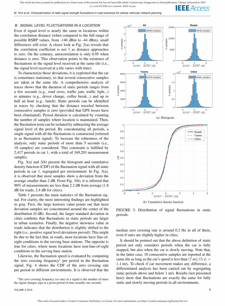
To characterize those deviations, it is exploited that the caris sometimes stationary, so that several consecutive samplesare taken at the same tile. A comprehensive analysis oftraces shows that the duration of static periods ranges froma few seconds (e.g., road cross, traffic jam, traffic light...)to minutes (e.g., driver change, coffee break...) and up tohalf an hour (e.g., lunch). Static periods can be identifiedin traces by checking that the distance traveled betweenconsecutive samples is zero (provided that GPS losses havebeen eliminated). Period duration is calculated by countingthe number of samples where location is maintained. Then,the fluctuation term can be isolated by subtracting the averagesignal level of the period. By concatenating all periods, asingle signal with all the fluctuations is constructed (referredto as fluctuation signal). To increase the robustness of theanalysis, only static periods of more than 5 seconds (i.e.,10 samples) are considered. This constraint is fulfilled by2,417 periods in car 1, with a total of 169,203 measurementsamples.

Fig. 3(a) and 3(b) present the histogram and cumulativedensity function (CDF) of the fluctuation signal with all staticperiods in car 1, segregated per environment. In Fig. 3(a),it is observed that most samples show a deviation from theaverage smaller than 2 dB. From Fig. 3(b), it is inferred that90% of measurements are less than 2.2 dB from average (1.8dB for roads, 2.4 dB for cities).

Table 1 presents the main statistics of the fluctuation sig-nal. For clarity, the most interesting findings are highlightedin gray. First, the large kurtosis value points out that mostdeviation samples are concentrated around the center of thedistribution (0 dB). Second, the larger standard deviation incities confirms that fluctuations in static periods are largerin urban scenarios. Finally, the negative skewness value inroads indicates that the distribution is slightly shifted to theright (i.e., positive signal level deviations prevail). This mightbe due to the fact that, in roads, most locations have line-of-sight conditions to the serving base stations. The opposite istrue for cities, where more locations have non-line-of-sightconditions to the serving base station.

Likewise, the fluctuation speed is evaluated by computingthe zero crossing frequency1 per period in the fluctuationsignal. Fig. 4 shows the CDF of the zero crossing rateper period in different environments. It is observed that the

1The zero crossing frequency (or rate) of a signal is the number of timesthe signal changes sign in a given period of time (usually one second).

All

-5 0 50

1

2

3

4

5

# sa

mpl

es

104

169203 samples

Roads

-5 0 50

5000

10000

15000

# sa

mpl

es

48766 samples

Towns

-5 0 50

2000

4000

6000

8000

# sa

mpl

es

32233 samples

Cities

-5 0 50

0.5

1

1.5

2

# sa

mpl

es

104

84481 samples

(a) Histogram.

-6 -4 -2 0 2 4 60

0.1

0.2

0.3

0.4

0.5

0.6

0.7

0.8

0.9

1

cdf

Roads Towns Cities

(b) Cumulative density function.

FIGURE 3: Distribution of signal fluctuations in staticperiods.

median zero crossing rate is around 0.2 Hz in all of them,even if rates are slightly higher in cities.

It should be pointed out that the above definition of staticperiod not only considers periods when the car is fullystopped, but also when the car is slowly moving. Note that,in the latter case, 10 consecutive samples are reported at thesame tile as long as the car’s speed is less than (7 m)/(5 s) =1.4 m/s. To check if car movement makes any difference, adifferentiated analysis has been carried out by segregatingstatic periods above and below 1 m/s. Results (not presentedhere) show that fluctuations are exactly the same for fullystatic and slowly moving periods in all environments.

VOLUME 4, 2016 5




TABLE 1: Statistics of signal fluctuation in static periods [dB].

Statistic/Environment All Roads Towns CitiesAverage 2.0 e-5 1.0 e-2 1.5 e-2 -6.0 e-5Standard deviation 2.042 1.317 1.362 2.501Median 0.024 0.058 0.023 0.015Skewness 1.41 -1.10 -0.35 1.54Kurtosis 42.6 16.33 11.25 35.32

0 0.1 0.2 0.3 0.4 0.5 0.6 0.7 0.8Zero crossing frequency [Hz]

0

0.1

0.2

0.3

0.4

0.5

0.6

0.7

0.8

0.9

1

cdf

Roads Towns Cities

FIGURE 4: Distribution of zero crossing frequency per pe-riod.

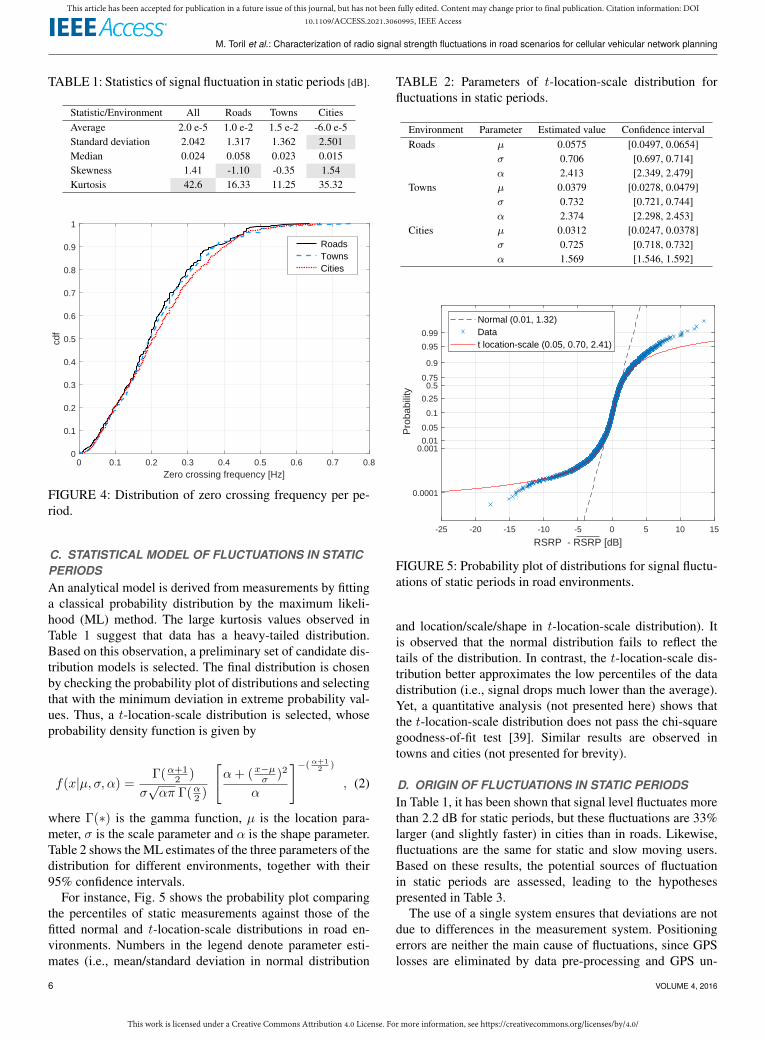
C. STATISTICAL MODEL OF FLUCTUATIONS IN STATICPERIODSAn analytical model is derived from measurements by fittinga classical probability distribution by the maximum likeli-hood (ML) method. The large kurtosis values observed inTable 1 suggest that data has a heavy-tailed distribution.Based on this observation, a preliminary set of candidate dis-tribution models is selected. The final distribution is chosenby checking the probability plot of distributions and selectingthat with the minimum deviation in extreme probability val-ues. Thus, a t-location-scale distribution is selected, whoseprobability density function is given by

f(x|µ, σ, α) =Γ(α+1

2 )

σ√απ Γ(α2 )

[α+ (x−µσ )2

α

]−(α+12 )

, (2)

where Γ(∗) is the gamma function, µ is the location para-meter, σ is the scale parameter and α is the shape parameter.Table 2 shows the ML estimates of the three parameters of thedistribution for different environments, together with their95% confidence intervals.

For instance, Fig. 5 shows the probability plot comparingthe percentiles of static measurements against those of thefitted normal and t-location-scale distributions in road en-vironments. Numbers in the legend denote parameter esti-mates (i.e., mean/standard deviation in normal distribution

TABLE 2: Parameters of t-location-scale distribution forfluctuations in static periods.

Environment Parameter Estimated value Confidence intervalRoads µ 0.0575 [0.0497, 0.0654]

σ 0.706 [0.697, 0.714]α 2.413 [2.349, 2.479]

Towns µ 0.0379 [0.0278, 0.0479]σ 0.732 [0.721, 0.744]α 2.374 [2.298, 2.453]

Cities µ 0.0312 [0.0247, 0.0378]σ 0.725 [0.718, 0.732]α 1.569 [1.546, 1.592]

-25 -20 -15 -10 -5 0 5 10 15

RSRP - RSRP [dB]

0.0001

0.0010.01

0.05

0.1

0.25

0.50.75

0.9

0.95

0.99

Pro

babi

lity

Normal (0.01, 1.32)Datat location-scale (0.05, 0.70, 2.41)

FIGURE 5: Probability plot of distributions for signal fluctu-ations of static periods in road environments.

and location/scale/shape in t-location-scale distribution). Itis observed that the normal distribution fails to reflect thetails of the distribution. In contrast, the t-location-scale dis-tribution better approximates the low percentiles of the datadistribution (i.e., signal drops much lower than the average).Yet, a quantitative analysis (not presented here) shows thatthe t-location-scale distribution does not pass the chi-squaregoodness-of-fit test [39]. Similar results are observed intowns and cities (not presented for brevity).

D. ORIGIN OF FLUCTUATIONS IN STATIC PERIODSIn Table 1, it has been shown that signal level fluctuates morethan 2.2 dB for static periods, but these fluctuations are 33%larger (and slightly faster) in cities than in roads. Likewise,fluctuations are the same for static and slow moving users.Based on these results, the potential sources of fluctuationin static periods are assessed, leading to the hypothesespresented in Table 3.

The use of a single system ensures that deviations are notdue to differences in the measurement system. Positioningerrors are neither the main cause of fluctuations, since GPSlosses are eliminated by data pre-processing and GPS un-

6 VOLUME 4, 2016




TABLE 3: Reasons for signal level fluctuations in static periods.

Reason ImpactMeasurement system differences (e.g., terminal, car, in-car position) NoPositioning errors (GPS losses, GPS uncertainty) NoChanges in far environment (e.g., weather, wind, temperature gradients) UnlikelyChanges in near environment (e.g., shadowing or reflection by nearby objects) YesMultipath fading (e.g., relative phase/strength of reflections) NoRadio resource management (e.g., handover to different serving cell) Unlikely

certainty (plus rounding) is reduced by the time constraintintroduced to define static periods, where samples must beconsecutive (i.e., measurements reported at the same locationdue to a location error, but taking place after the end of theperiod, are discarded). Likewise, should the far environmentbe the source of fluctuations, these would be larger in openroads, where distance to the base station is larger. Similarly,if multipath fading exists (because tile size was not largeenough to remove its effect), fluctuations at the same tilewould have to be larger for slowly moving users than forstatic users. Recall that tile resolution is 7 meters (i.e.,43 times the wavelength at 1847 MHz). Finally, it is veryunlikely that a static user changes serving cell. For all thesereasons, it is expected that signal fluctuations for static usersare mainly due to changes in the near environment (e.g.,temporal shadowing by a pedestrian or another vehicle).

V. DUAL-SYSTEM ANALYSISThe following paragraphs describe the comparison of mea-surements from the two cars. Hereafter, system 1 denotes theSamsung Galaxy S10 handset in car 1 and system 2 denotesthe Samsung Galaxy S10 handset in car 2.

The aim is to check signal differences when cars are atthe same tile. For this purpose, tiles crossed by the two carsare identified from traces. Note that, even if both cars followsimilar routes, small path differences may still exist (e.g.,different lane in the highway). Likewise, sampling at 2 Hz(i.e., period of 0.5 s) causes that car trajectory on the mapis discontinuous when the car is traveling at high speeds. Asshown in Fig. 1, points consecutive in the trace may be 3-4 tiles apart on the map in highways. Likewise, positioningerrors due to GPS uncertainty and rounding may occasionallymove the point to the adjacent tile. All these factors makethat only a small set of points in both traces share exactlythe same location. Specifically, 96,443 common samples (outof 593,858 in car 1 and 661,521 in car 2) are found afterpre-processing (i.e., approximately 15%). Nonetheless, thedataset is large enough to provide significant results.

In each tile, signal level, instantaneous car speed andtime lapse between measurements are computed. To discardany difference between the measurement systems installedon the two cars, Fig. 6 shows a scatter plot of the signallevel received by the cars at the same tile. It is observedthat RSRP measurements are strongly correlated betweensystems, evident from the high value of the sample determi-

y = - 5.81+ 0.93 x

R2 = 0.89

A

B

FIGURE 6: Correlation between measurements from cars atthe same location.

nation coefficient (R2 = 0.89). Likewise, the slope of theregression curve is nearly 1, without any significant bias onthe range of interest. Nonetheless, significant deviations areobserved in some tiles (highlighted by arrows).

To break down these deviations, Fig. 7 (a)-(b) show thehistogram and CDF of their distribution. For comparisonpurposes, in Fig. 7(b), the CDF of fluctuations for static usersis also superimposed. At first sight, it is clear that deviationsbetween the 2 cars are much larger than fluctuations forstatic users. Specifically, the 5th and 95th percentiles of thedistribution of signal differences between systems are −6.5and 6.2 dB, respectively, compared to −2.3 and 2.1 dBfor fluctuations in static users (i.e., 4 dB larger). Closeranalysis (not presented here) confirms that the magnitude offluctuations does not depend on the time lapse between themeasurements of both systems (neither when time differenceis in the order of seconds nor hours).

Fig. 8 shows the CDF of signal level differences betweensystems per environment. It is observed that larger positivedeviations exist on roads, whereas larger negative deviationsoccur in cities. This result is just a consequence of thedifferent skewness factors, already observed when analyzingthe measurements of car 1 in Table 1.

VOLUME 4, 2016 7




-20 -15 -10 -5 0 5 10 15 20

RSRP syst2 - RSRP syst1 [dB]

0

1000

2000

3000

4000

5000

6000

7000

#sam

ples

Avg RSRP diff [dB]:-0.24282

(a) Histogram.

-20 -15 -10 -5 0 5 10 15 20


0

0.1

0.2

0.3

0.4

0.5

0.6

0.7

0.8

0.9

1

cdf

syst2 vs syst1syst1 (same location)

(b) Cumulative density function.

FIGURE 7: Distribution of signal level differences betweenco-located systems.

A. STATISTICAL MODEL OF DIFFERENCES BETWEENCARSAs for static users, an analytical model is derived for signallevel differences between cars by fitting a probability distri-bution selected a priori. In this case, a logistic distribution ischosen, whose probability density function is given by

f(x|µ, σ) =e−

x−µσ

σ (1 + e−x−µσ )2

, (3)

where µ is the location parameter and σ is the scale para-meter. Table 4 shows the ML estimates of the logistic param-eters in the different environments.

Fig. 9 shows the probability plot with percentiles ofmeasurements and fitted distributions for signal differencesbetween cars in road environments. As for fluctuations in

-10 -8 -6 -4 -2 0 2 4 6 8 10RSRP syst2 - RSRP syst1 [dB]

0

0.1

0.2

0.3

0.4

0.5

0.6

0.7

0.8

0.9

1

cdf

RoadsTownsCities

FIGURE 8: Signal level differences between co-located sys-tems per environment.

TABLE 4: Parameters of logistic distribution for differencesbetween co-located systems per environment.

Environment Parameter Estimated value Confidence intervalRoads µ 0.0575 [0.0497, 0.0654]

σ 0.706 [0.697, 0.714]Towns µ 0.0379 [0.0278, 0.0479]

σ 0.732 [0.721, 0.744]Cities µ 0.0312 [0.0247, 0.0378]

σ 0.725 [0.718, 0.732]

static users, the normal distribution fails to reflect the tailsof the distribution of signal differences between cars at thesame location. In contrast, the logistic distribution closelyapproximates the data distribution for extreme percentiles,even if it neither passes the chi-square goodness-of-fit test.Again, the same trends are observed in towns and cities (notpresented for brevity).

B. ORIGIN OF DIFFERENCES BETWEEN CARSTo unveil the origin of extreme deviations, a more detailedanalysis of outliers is carried out. In particular, the analysisis focused on the 2 points highlighted in Fig. 6, showing verylarge positive and negative differences between cars.

The outlier A on the upper-left of the figure has−111 dBmfor system 1 and −92 dBm for system 2 (19 dB deviation).Fig. 10 (a)-(c) present a detailed analysis of the trace, signallevel and speed of both cars around the event. For ease ofanalysis, in the photo in Fig. 10(a), the trace followed by eachof the car is depicted in a different color, highlighting com-mon points. Likewise, signal level and speed in Fig. 10(b) and10(c) are not presented against time, but location (latitude),since both cars can move at different speeds, as deducedfrom Fig. 10(c). Note that the time axis goes from right toleft, as cars are heading south (i.e., decreasing latitude). In

8 VOLUME 4, 2016




-25 -20 -15 -10 -5 0 5 10 15 20 25


0.0001

0.001

0.01

0.050.1

0.25

0.5

0.75

0.90.95

0.99

0.999

0.9999

Pro

babi

lity

Normal (-0.26, 4.07)DataLogistic (-0.31, 2.23)

FIGURE 9: Probability plot of distributions for signaldeviations between co-located systems in road environments.

Fig. 10(a), it is observed that both trajectories coincide inmany points. A closer inspection of the orthophoto showsthat the analyzed road segment is surrounded by naturalwalls, which causes an obstruction of the line of sight tothe serving base station. Such an event is also evident inFig. 10(b), where it is observed that signal level decreasesfrom−105 to−110 dBm at the beginning of the trace (right)in both systems. From that point, both systems differ. System1 experienced a large increase of signal level, while system2 experiences a similar increase but 3 samples (1.5 s) later.Thereafter, both systems follow a similar trend. A carefulinspection of traces shows that the abrupt change in signallevel is due to a change of serving cell (i.e., handover). Incase of system 1, the handover to the new (stronger) cell isdelayed a few seconds for some reason (e.g., new base stationtemporarily shadowed by another vehicle).

A similar phenomenon is observed in the outlier B atlower-right of the curve in Fig. 6. In this case, system 1displays −76.5 dBm and system 2 −102 dBm (23.5 dBdeviation). Fig. 11 (a)-(c) again show the trace, signal leveland car speed associated to the event. The orthophoto inFig. 11(a) shows a road cross surrounded by houses in a sub-urban area of a city. Note that, in this case, the 2 cars followcompletely different routes, intersecting in a single commonlocation. From Fig. 11(c), it is inferred that car 1 stops at thecross (as speed becomes zero), while car 2 does not stop.More importantly, it is observed that none of the systemschanges signal level as they go through the cross, even if thesignal received by system 1 at the common location is manydecibels above that of system 2. Such a difference comesfrom a different serving cell. It is hypothesized that system2 does not trigger a handover to the cell serving system 1because it traverses the cross at more than 50 km/h.

Based on the above observations, Table 5 summarizes thehypotheses on the origin of deviations for moving users. The

reasons for the larger differences compared to static users arehighlighted in gray. Deviations are not due to measurementsystems, because both use the same handset model andare located at the same position in the car (rear window).However, location errors are larger than for static users, asno time constraint is considered when selecting the pair ofmeasurements to be compared. It was shown in Fig. 1(b) thatGPS uncertainty and latitude/longitude rounding may takea measurement to the adjacent tile, 7 meters away. In thevicinity of small obstacles (e.g., vehicle, tree, signboard...),such a small distance is the difference between being in lineof sight or not to the base station. Therefore, it is expectedthat positioning errors are the main reason behind the 4 dBlarger 95th tile compared to fluctuations of static users. More-over, the outlier analysis has shown that extreme deviationsare normally due to handover procedures, causing that thetwo systems, traveling at different speeds (and sometimes indifferent directions), are not served by the same cell. Sucha handover behavior is influenced by network settings (e.g.,hysteresis and timers), operator policy (e.g., default carrierfor certain services) or network hierarchy (e.g., target basestation assigned to a different core network element).

VI. CONCLUSIONSUnderstanding the fluctuations of the radio signal receivedby mobile users at a certain location is key for setting theright safety margins in cellular network planning. Such apiece of information will be important in road scenarios forapplications that require ultra-reliable low-latency commu-nications. In this work, a comprehensive analysis of radiosignal strength fluctuations on roads in a LTE system hasbeen presented. The analysis is based on a nationwide drivetest with 2 cars sharing the same measurement system.

The analysis of measurements from one of the cars hasshown that correlation distance is 710 m in open roads and430 m in towns and cities. These values can be used todefine the spatial grid resolution in radio network planningtools for road coverage scenarios. Defining tile size abovecorrelation distance is a waste of computational resources,whereas defining it below might cause that coverage issuesare not detected due to lack of spatial detail. Moreover, theanalysis of static periods has shown fluctuations around 1.8and 2.2 dB in roads and cities, respectively. These deviationsare mostly due to changes in shadowing conditions caused byother vehicles.

The comparison of measurements between cars has showntypical deviations of more than 6 dB in all road scenarios.Even if part of these deviations are due to positioning errorsin the measurement system, these highlight an importantissue, which is the fact that adjacent tiles separated only a fewmeters may have different coverage levels. Thus, differentlanes on the road would receive different signal levels fromthe serving cell (typical lane width is around 3.5 m). Alsoimportant, extreme deviations of more than 23 dB havebeen observed at the same location caused by differences inthe serving cell due to handover procedures. It is expected

VOLUME 4, 2016 9




TABLE 5: Reasons for signal level differences between co-located systems.

Reason ImpactMeasurement system differences (e.g., terminal, car, in-car position) NoPositioning errors (GPS losses, GPS uncertainty) Yes (normal)Changes in far environment (e.g., weather, wind, temperature gradients) UnlikelyChanges in near environment (e.g., shadowing or reflection by nearby objects) YesMultipath fading (e.g., relative phase/strength of reflections) NoRadio resource management (e.g., handover to different serving cell) Yes (extreme)

that deviations will be even larger for real users, since theyhave different handset models, vehicle class and pathlossenvironment inside vehicle (e.g., pocket, glovebox...).

The risk of neglecting those extreme signal fluctuations isunderestimating propagation losses. This action would leadto an optimistic maximum cell radius in network dimen-sioning and overconfident performance predictions in radionetwork planning for services requiring high reliability inroads. Ultimately, both effects might degrade the perfor-mance of ultra-reliable low-latency services needed for con-nected car applications in live 5G systems. This problem canbe avoided by increasing safety margins in the link budgetof these services. It should be pointed out that, even if allthese deviations negatively affect network costs as more basestations are needed, they add diversity to C-V2N communica-tions, which can be exploited by the multiconnectivity featurein 5G to achieve more reliable links.

Future work will repeat the tests with different handsets(4G-only vs 5G-capable), services (voice vs data), bands(800/1800/2100/2600 MHz, 3.5/26 GHz) and radio accesstechnologies (4G vs 5G). These tests will check to whichextent the results presented here can be generalized. It isenvisaged that the influence of the specific measurementsetup (e.g., terminal, in-car position, etc.) should be small,provided that the same setup is maintained in the two cars.Even if this was not the case, the values derived for modelparameters correspond to a typical situation. Nonetheless,it would be interesting to characterize deviations due to in-car losses (different cars or different positions inside car)and synchronization issues when handsets are at the samecar. In 5G systems, it would be expected that similar resultsare obtained, provided that the same frequency is used.However, preliminary tests have shown that terminal andservice diversity causes extreme signal deviations at the samelocation (> 50 dB) due to the traffic management policy ofthe operator. For example, a user at the same location mightbe served by different carriers depending on the requestedservice. Likewise, certain handsets might be pushed to orkept in different frequency bands / technology layers. Suchoccurrences are associated with the rollout of a new radiotechnology and are likely to disappear once it is deployedwidely across the network. Also, in the millimeter band,severe weather conditions (e.g., rain or fog) and higherpenetration losses (due to, e.g., metalized car windows) willincrease the magnitude of fluctuations.

REFERENCES[1] “5G White Paper,” NGMN, white paper, 2015.[2] “Connecting cars on the road to 5G,” Huawei, white paper, 2017.[3] https://www.alliedmarketresearch.com/connected-car-market (last

accessed on 23/07/20).[4] C. Boberg, M. Svensson, and B.Kovacs, “Distributed cloud, automotive

and industry 4.0,” Ericsson Technology Review, no. 11, pp. 1–12, Nov.2018.

[5] Study on LTE-based V2X Services (Release 14), 3GPP TR 36.885, v14.0.0Std., Jun. 2015.

[6] Study on architecture enhancements for the Evolved Packet System (EPS)and the 5G System (5GS) to support advanced V2X services, 3GPP TR23.786, v16.1.0 Std., Jun. 2019.

[7] “Tranforming transportation with 5G,” Ericsson, white paper, 2019.[8] “5G Automotive vision,” 5G-PPP, white paper, 2015.[9] F. J. Martin-Vega, M. C. Aguayo-Torres, G. Gomez, J. T. Entrambasaguas,

and T. Q. Duong, “Key technologies, modeling approaches, and challengesfor millimeter-wave vehicular communications,” IEEE CommunicationsMagazine, vol. 56, no. 10, pp. 28–35, Oct. 2018.

[10] C. Chen, B. Wang, and R. Zhang, “Interference hypergraph-based resourceallocation (IHG-RA) for NOMA-integrated V2X networks,” IEEE Internetof Things Journal, vol. 6, no. 1, pp. 161–170, Feb. 2019.

[11] W. Xu, H. Zhou, H. Wu, F. Lyu, N. Cheng, and X. Shen, “Intelligent linkadaptation in 802.11 vehicular networks: Challenges and solutions,” IEEECommunications Standards Magazine, vol. 3, no. 1, pp. 12–18, Mar. 2019.

[12] X. Li, L. Ma, Y. Xu, and R. Shankaran, “Resource allocation for D2D-based V2X communication with imperfect CSI,” IEEE Internet of ThingsJournal, vol. 7, no. 4, pp. 3545–3558, Apr. 2020.

[13] J. Mei, X. Wang, and K. Zheng, “Intelligent network slicing for V2Xservices toward 5G,” IEEE Network, vol. 33, no. 6, pp. 196–204, Nov.2019.

[14] F. Giust, V. Sciancalepore, D. Sabella, M. C. Filippou, S. Mangiante,W. Featherstone, and D. Munaretto, “Multi-access edge computing: Thedriver behind the wheel of 5G-connected cars,” IEEE CommunicationsStandards Magazine, vol. 2, no. 3, pp. 66–73, Sep. 2018.

[15] J. Zhang and K. B. Letaief, “Mobile edge intelligence and computing forthe internet of vehicles,” Proceedings of the IEEE, vol. 108, no. 2, pp.246–261, Feb. 2020.

[16] H. Zhou, W. Xu, J. Chen, and W. Wang, “Evolutionary V2X technologiestoward the internet of vehicles: Challenges and opportunities,” Proceed-ings of the IEEE, vol. 108, no. 2, pp. 308–323, Feb. 2020.

[17] K. Strandberg, T. Olovsson, and E. Jonsson, “Securing the connectedcar: A security-enhancement methodology,” IEEE Vehicular TechnologyMagazine, vol. 13, no. 1, pp. 56–65, Mar. 2018.

[18] “A study on 5G V2X deployment,” 5G-PPP, white paper, Feb. 2018.[19] “C-ITS vehicle to infrastructure services: how C-V2X technology com-

pletely changes the cost equation for road operators,” 5GAA, white paper,Jan. 2019.

[20] Y. Yang and K. Hua, “Emerging technologies for 5G-enabled vehicularnetworks,” IEEE Access, vol. 7, pp. 181 117–181 141, Dec. 2019.

[21] T. Rappaport, Wireless Communications: Principles and Practice, 2nd ed.USA: Prentice Hall PTR, 2001.

[22] P. Kyosti et al., “WINNER II channel models, WINNER II D1.1.2 v1.1,Tech. Rep., 2007.

[23] Study on channel model for frequencies from 0.5 to 100 GHz (Release 16),3GPP TR 38.901, v6.1.0 Std., Dec. 2019.

[24] M. Gudmundson, “Correlation model for shadow fading in mobile radiosystems,” Electronics Letters, vol. 27, no. 23, pp. 2145–2146, 1991.

[25] K. Siwiak, Radiowave Propagation and Antennas for Personal Communi-cations. Artech House, 1995.

10 VOLUME 4, 2016




[26] S. Saunders and A. Aragon-Zavala, Antennas and Propagation for Wire-less Communication System, 2nd ed. Wiley, 2007.

[27] J. Monserrat, R. Fraile, D. Calabuig, and N. Cardona, “Complete shadow-ing modeling and its effect on system level performance evaluation,” inIEEE Vehicular Technology Conference, May 2008, pp. 294 –298.

[28] J. Weitzen and T. J. Lowe, “Measurement of angular and distance correla-tion properties of log-normal shadowing at 1900 MHz and its applicationto design of PCS systems,” IEEE Transactions on Vehicular Technology,vol. 51, no. 2, pp. 265–273, Mar. 2002.

[29] A. Mishra, Fundamentals of cellular network planning and optimisation,2nd ed. Wiley, 2018.

[30] P. Agrawal and N. Patwari, “Correlated link shadow fading in multi-hop wireless networks,” IEEE Transactions on Wireless Communications,vol. 8, no. 8, pp. 4024–4036, Aug. 2009.

[31] R. Inam, N. Schrammar, K. Wang, A. Karapantelakis, L. Mokrushin,A. V. Feljan, and E. Fersman, “Feasibility assessment to realise vehicleteleoperation using cellular networks,” in 2016 IEEE 19th InternationalConference on Intelligent Transportation Systems (ITSC), Nov. 2016, pp.2254–2260.

[32] S. Neumeier, E. A. Walelgne, V. Bajpai, J. Ott, and C. Facchi, “Measuringthe feasibility of teleoperated driving in mobile networks,” in 2019 Net-work Traffic Measurement and Analysis Conference (TMA), Jun. 2019, pp.113–120.

[33] A. Gaber, W. Nassar, A. M. Mohamed, and M. K. Mansour, “Feasibilitystudy of teleoperated vehicles using multi-operator LTE connection,” in2020 International Conference on Innovative Trends in Communicationand Computer Engineering (ITCE), Mar. 2020, pp. 191–195.

[34] M. Lauridsen, T. Kolding, G. Pocovi, and P. Mogensen, “Reducing han-dover outage for autonomous vehicles with LTE hybrid access,” in 2018IEEE International Conference on Communications (ICC), May 2018, pp.1–6.

[35] U. Saeed, J. Hamalainen, E. Mutafungwa, R. Wichman, D. Gonzalez,and M. Garcia-Lozano, “Route-based radio coverage analysis of cellularnetwork deployments for V2N communication,” in 2019 InternationalConference on Wireless and Mobile Computing, Networking and Commu-nications (WiMob), Oct. 2019, pp. 1–6.

[36] M. Lauridsen, L. C. Gimenez, I. Rodriguez, T. B. Sorensen, and P. Mo-gensen, “From LTE to 5G for connected mobility,” IEEE CommunicationsMagazine, vol. 55, no. 3, pp. 156–162, Mar. 2017.

[37] S. Shetty, S. Lackovic, and S. Z. Pilinsky, “4G coverage analysis ofCroatian main roads,” in 2017 International Symposium ELMAR, Sep.2017, pp. 129–132.

[38] “The 2019 mobile network in Spain,” Umlaut, Tech. Rep., 2020.[39] W. Navidi, Statistics for Engineers and Scientists. McGraw-Hill Higher

Education, 2004.

MATÍAS TORIL received his M.S. in Telecommu-nication Engineering and Ph.D. degrees from theUniversity of Málaga, Spain, in 1995 and 2007, re-spectively. Since 1997, he is Lecturer in the Com-munications Engineering Department, Universityof Málaga, where he is currently Full Professor.He has co-authored more than 150 publicationsin leading conferences and journals and 8 patentsowned by Nokia and Ericsson. His current re-search interests include self-organizing networks,

radio resource management and data analytics.

VOLKER WILLE received the B.S. degree fromthe University of Applied Sciences and Arts ofHannover, Hannover, Germany, in 1991, and thePh.D. degree from the University of Glamorgan,Cardiff, U.K., in 1995. He was an Intern withBell Communications Research, Morristown, NJ,USA. He is currently with Nokia, Huntingdon,U.K., where he is involved in the optimization ofcellular networks.

SALVADOR LUNA-RAMÍREZ received his M.S.in Telecommunication Engineering and Ph.D. de-grees from the University of Málaga, Spain, in2000 and 2010, respectively. Since 2000, he hasbeen with the Communications Engineering De-partment, University of Málaga, where he is cur-rently Associate Professor. His research interestsinclude self-optimization of mobile radio accessnetworks and radio resource management.

MARIANO FERNÁNDEZ-NAVARRO receivedhis M.S. in Telecommunication Engineering fromthe Polytechnic University of Madrid in 1988 andthe Ph.D. degree from the University of Málagain 1999. He is on the staff of the Communica-tions Engineering Department at the University ofMálaga since 1992, after 3 years as design engi-neer at Fujitsu Spain S.A. His research interests in-clude optimization of radio resource managementfor mobile networks and location-based services

and management.

FERNANDO RUIZ-VEGA received his M.S. inTelecommunication Engineering from the Univer-sity of Málaga, Spain, in 1994. After working inCETECOM testing laboratory with type-approvaltest systems for communication equipment, hejoined the Communications Engineering Depart-ment of the University of Málaga, where, in 2001,he became Associate Professor. In 1995, he was aVisiting Researcher with the Department of Elec-trical Engineering and Electronics, University of

Liverpool, Liverpool, UK. From 2000 to 2002, he took part in the NokiaMobile Communications Competence Centre, Málaga, Spain. His researchinterests include mobile radio propagation channel characterization andemulation.

VOLUME 4, 2016 11




Car 1 Car 2 Car 1&2

Natural walls

(a) Trace.

51.184 51.1845 51.185 51.1855 51.186 51.1865

Lat[º]

-115

-110

-105

-100

-95

-90

Syst1Syst2

Time

19 dB

(b) Signal level.

51.184 51.1845 51.185 51.1855 51.186 51.1865

Lat[º]

96

98

100

102

104

106

108

110

112

114

Spe

ed[k

m/h

]

Syst1Syst2

(c) Car speed.

FIGURE 10: Analysis of outlier 1 (natural wall corridor).

Car 1 Car 2 Car 1&2

Road cross

(a) Trace.

52.5351 52.5352 52.5353 52.5354 52.5355 52.5356 52.5357 52.5358

Lat[º]

-110

-105

-100

-95

-90

-85

-80

-75

-70

-65

RSRP[dBm]

Syst1Syst2

23.5 dB

(b) Signal level.

52.5351 52.5352 52.5353 52.5354 52.5355 52.5356 52.5357 52.5358

Lat[º]

0

10

20

30

40

50

60

70

80

Spe

ed[k

m/h

]

Syst1Syst2

(c) Car speed.

FIGURE 11: Analysis of outlier 2 (road cross).

12 VOLUME 4, 2016

characterization of radio signal strength fluctuations in

Documents