characterizing agent behavior under meta reinforcement

CHARACTERIZING AGENT BEHAVIOR UNDER META

REINFORCEMENT LEARNING WITH GRIDWORLD

A Senior Honors Thesis Presented to

the Faculty of the Department of Computer Science

University of Houston

In Partial Fulfillment

of the Requirements for the Degree

Bachelors of Science

By

Nolan Shah

December 2018



Nolan Shah

APPROVED:

Dr. Ricardo Vilalta, ChairmanDept. of Computer Science

Dr. Weidong (Larry) ShiDept. of Computer Science

Dr. Peggy LindnerHonors College

Dr. Dan Wells, DeanCollege of Natural Sciences and Mathematics

ii

Acknowledgments

I am very grateful to Dr. Ricardo Vilalta for his encouragement, guidance, and mentorship.

I would not have been able to learn so much if not for his support. I am also grateful to

Dr. Weidong (Larry) Shi for providing computational resources and his constant support. I

would also like to give thanks to Dr. Peggy Lindner for her feedback throughout this work.

I have had the opportunity to fail a thousand times over, and the good fortune of having

so many professors, mentors, friends, and family who have given me the opportunity to

keep moving forward. Special thanks to Dr. Vilalta, Dr. Shi, Dr. Omprakash Gnawali,

Mr. Abraham Baez-Suarez, the whole I2C Lab, and so many others in the Department of

Computer Science and the Honors College for making the past few years so memorable.

iii



An Abstract of a Senior Honors Thesis

Presented to

the Faculty of the Department of Computer Science

University of Houston

In Partial Fulfillment

of the Requirements for the Degree

Bachelors of Science

By

Nolan Shah

December 2018

iv

Abstract

The capabilities of meta reinforcement learning agents tend to be heavily depend on the

complexity and scope of the meta task over which they perform requiring different models,

learning algorithms, and strategies to perform well. In this thesis, we show the fragility

of agent design and limitations of agents across Gridworld-based meta tasks of increasing

complexity. We begin by building a characterization of the complexity of meta tasks within

a domain generalization context. We run experiments that demonstrate the ability of agents

to perform effectively on meta tasks parameterized with different environmental states, but

similar underlying rules. Next, we perform experiments that expose the limitations of those

same agents over tasks with different underlying rules, but similar observational spaces.

These experiments show that generalization-based strategies succeed with meta tasks that

sample from a small scope of base tasks with similar underlying rules, but break beyond

that complexity. We also infer from observed agent behaviors that the limitations of agents

are attributable to the nature of the model architecture and the meta task design. Further-

more, we run experiments that identify the sensitivity of agent behavior to physical features

by augmenting the agent observation size. These experiments show a resilience to limited

environmental information, but a lack of spatial awareness to abundant environmental in-

formation. Overall, this work provides a baseline for meta reinforcement learning with

the Gridworld task and exposes the necessary considerations of agent and environmental

design.

v

Contents

1 Introduction 1

2 Preliminaries 4

2.1 Deep Reinforcement Learning . . . . . . . . . . . . . . . . . . . . . . . . 4

2.1.1 Deep Q-Learning . . . . . . . . . . . . . . . . . . . . . . . . . . . 6

2.1.2 REINFORCE . . . . . . . . . . . . . . . . . . . . . . . . . . . . . 8

2.2 Meta Learning . . . . . . . . . . . . . . . . . . . . . . . . . . . . . . . . . 9

2.3 Meta Reinforcement Learning . . . . . . . . . . . . . . . . . . . . . . . . 12

3 Methods 13

3.1 Gridworld Base Tasks . . . . . . . . . . . . . . . . . . . . . . . . . . . . . 13

3.2 Meta Tasks . . . . . . . . . . . . . . . . . . . . . . . . . . . . . . . . . . 16

3.2.1 Parameterized Meta Task . . . . . . . . . . . . . . . . . . . . . . . 16

3.2.2 Extended Parameterized Meta Task . . . . . . . . . . . . . . . . . 17

3.3 Experimental Design . . . . . . . . . . . . . . . . . . . . . . . . . . . . . 19

3.3.1 Learning Algorithm & Model Architecture . . . . . . . . . . . . . 20

3.3.2 Observation Window . . . . . . . . . . . . . . . . . . . . . . . . . 21

4 Results 23

4.1 Learning Algorithm & Model Architecture . . . . . . . . . . . . . . . . . . 23

vi

4.2 Observation Window . . . . . . . . . . . . . . . . . . . . . . . . . . . . . 34

5 Conclusion 37

vii

Chapter 1

Introduction

A cornerstone of human behavior is the ability to adapt to a wide variety of tasks using sim-

ilar physical movements and behaviors. For example, we can switch between variations of

the sport of soccer, between a full-scale professional game with 22 players to a very sim-

ple game of kick-the-ball with only one player. We automatically take into consideration

physical constraints, conceptual rules, and contextual clues of the games, so that adapting

between games becomes very natural. This is the essence of meta learning.

Meta learning, like many other fields of machine learning, has developed out of attempt-

ing to build machines with human-behavioral abilities. Within the context of reinforcement

learning, a meta learner is a complex decision making agent with relevant domain knowl-

edge and the ability to evaluate task strategies to adapt to similar, but novel tasks. More

formally, meta learners are characterized by three distinct abilities: (1) compare and evalu-

ate learning methods, (2) measure the benefits of early learning on subsequent learning, and

(3) use such evaluations to reason about learning strategies to select ”useful” ones, while

discarding others [18].

Meta learners come in many forms, with nearly all following this characterization in

one way or another. Some meta learners are built to improve the efficiency of learning

1

novel variants of a previous task, some to generalize over a variety of tasks, and some even

to learn the process of learning itself. These variants are referred to in the literature by

many names including algorithm selection, transfer learning, multi-task learning, learning-

to-learn, and domain adaptation.

With advancements in deep learning, which utilizes function approximators in deep

neural network architectures, meta learners have become increasingly sophisticated, en-

abling good performance on complex reinforcement learning tasks such as Atari video

games and motor control. Only recently has meta learning begun to catch up with advance-

ments in deep learning, through research in transfer learning in the contexts of supervised

and reinforcement learning [5], and in learning-to-learn, which exploits the temporal con-

nections of recurrent neural networks to adapt to new tasks [22, 4].

Even though there have been significant advancements in learning performance partic-

ularly with deep meta reinforcement learning, the increasing sophistication makes analy-

sis of agent behavior (to identify root cause or shape agent behavior in a particular way)

more difficult to achieve, especially as agents are trained over tasks using gradient descent

methods. The study of agent behavior and the internal dynamics of agents is necessary

to identify the progress made towards our original goal of building machines with human

behavioral abilities.

With this in mind, this work seeks to study agent behavior to identify their abilities and

limitations within a meta learning context. We begin by defining a formalism to describe

the complexity and degree of similarity between meta-learning tasks. Using this founda-

tion, we define five Gridworld environments which provide a series of versatile base tasks

that are used to define the Parameterized Meta Task (PMT) and the Extended Parameterized

Meta Task (EPMT) which are two meta tasks with different levels of difficulty. We then

define agents based on state-of-the-art research and benchmark their performances over

the PMT and EPMT tasks providing both quantitative results and a qualitative behavioral

2

analysis of agents. Finally, we analyze agent performance on changes to the agent obser-

vational window to show the fragility of agent performance under nuanced changes to the

experimental design.

This work is organized in the following chapters. Chapter 2 lays out the relevant back-

ground, related work, and meta-learning foundations. Chapter 3 describes the five Grid-

world base tasks, two meta tasks, agent designs, and experiments performed. In Chapter

4, we give experimental results, observations, and analysis. Finally, we conclude in Chap-

ter 5.

3

Chapter 2

Preliminaries

2.1 Deep Reinforcement Learning

Reinforcement Learning (RL) is an area of machine learning concerned with sequential

decision problems where a learning agent must learn to interact with its environment

to achieve a goal [20]. Reinforcement learning is usually applied over tasks that can

be modeled as Markov Decision Processes (MDP) [20]. Formally, an MDP is a tuple

(S,A, Pa, Ra, �) where S is a finite set of states, A is a finite set of actions, Pa(s, s0) is the

probability that action a in state s at time t will lead to state s0, Ra(s, s0) is the expected im-

mediate reward received after transitioning from state s to state s0 due to action a, and � is

the discount factor, which represents the difference in importance between future rewards

and present rewards. For simplicity, we will constrain our study to finite-horizon MDPs.

Reinforcement Learning algorithms aim to find a policy ⇡ that specifies the probability

⇡(a|s) of an agent selecting action a when in state s to maximize a reward. The objective of

maximizing reward is formulated as maximizing the expected sum of discounted rewards

over time

Gt = E[TX

t

�trt],

4

where T is the finite horizon. To assist in this objective, many reinforcement learning

algorithms involve estimating a state-value function

v⇡(s) = E[Gt|St = s],

that estimates how ”good” it is to be in state s. A similar function exists called the action-

value function

q⇡(s, a) = E[Gt|St = s, At = a],

that estimates how ”good” it is to take action a while in state s.

There are three main classes of reinforcement learning algorithms: value function meth-

ods, policy search methods, and actor-critic methods [3]. Value function methods are based

on the principle that the optimal policy has a corresponding optimal value function, so by

greedily choosing the action with the greatest value, we can generate an optimal policy.

Some examples of value function methods are Q-learning [13] and SARSA [1]. Policy

search methods do not maintain a value function, instead searching directly for an optimal

policy. This is usually performed by parameterizing the policy and using dynamic pro-

gramming, or some other optimization technique, to find the optimal policy. An example

of a policy search method is REINFORCE [24]. The final actor-critic method is a hybrid

of value function and policy search composed of an ”actor” (policy) that learns using feed-

back from the ”critic” (value function). The result is a trade-off that reduces variance of the

policy gradients, but introduces bias from the value function [9].

In recent years, these reinforcement learning methods have scaled up to high dimen-

sional sensory inputs and complex internal control logic by using deep learning-based func-

tion approximators such as neural networks. These function approximators learn feature

representations as well as various kinds of abstractions and approximations that effectively

handle sophisticated tasks by creating sufficient internal complexity to handle high dimen-

5

sional observational spaces. New types of deep neural networks such as convolutional

neural networks (CNNs) and recurrent neural networks (RNNs) have led to flexibility in

exploiting spatial and temporal relations in data. The use of deep learning has enabled

state-of-the-art performance over supervised learning tasks such as speech recognition and

image classification [10], and reinforcement learning tasks such as motor control [12, 19]

and playing Atari games [3].

We introduce two deep reinforcement learning algorithms relevant to this work: Deep

Q-Learning and REINFORCE.

2.1.1 Deep Q-Learning

Q-Learning is a model-free off-policy algorithm for estimating the expected long-term re-

turn of executing an action from a given state [23]. These estimated returns are known as

Q-values. The optimal action-value function is

Q⇤(s, a) = max⇡E[rt + �rt+1 + �2rt+2 + ...|st = s, at = a, ⇡].

As Q-Learning is an off-policy algorithm, we can generate separate target and behavior

policies. The target policy is the learned policy which is used when evaluating the agent’s

performance. At a given state, it selects the action with the maximal Q-value. The behavior

policy derived from the target policy improves exploration during training; it uses decayed

✏-greedy action selection over Q-values.

In practice, Q-values are learned iteratively by updating the current Q-value estimate

with the observed reward and the maximum Q-value over all actions a0 in the resulting state

s0. The update function is

Qt(s, a) = Qt�1(s, a) + ↵(r + �maxa0Q(s0, a0)�Q(s, a)).

6

Historically, Q-Learning has had difficulties with many challenging domains, including

video games, because of the vast number of states that make it too difficult to maintain a

separate estimate for each state-action pair. Deep Q-Learning [13] seeks to solve many of

these difficulties by approximating Q-values with a deep neural network. At each iteration,

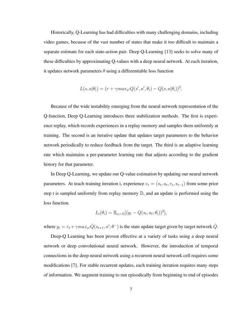
it updates network parameters ✓ using a differentiable loss function

L(s, a|✓i) = (r + �maxa0Q(s0, a0, ✓i)�Q(s, a|✓i))2.

Because of the wide instability emerging from the neural network representation of the

Q-function, Deep Q-Learning introduces three stabilization methods. The first is experi-

ence replay, which records experiences in a replay memory and samples them uniformly at

training. The second is an iterative update that updates target parameters to the behavior

network periodically to reduce feedback from the target. The third is an adaptive learning

rate which maintains a per-parameter learning rate that adjusts according to the gradient

history for that parameter.

In Deep Q-Learning, we update our Q-value estimation by updating our neural network

parameters. At teach training iteration i, experience et = (st, at, rt, st�1) from some prior

step t is sampled uniformly from replay memory D, and an update is performed using the

loss function

Li(✓i) = Eet⇠D[(yi �Q(st, at; ✓i))2],

where yi = rt+�maxa0Q(st+1, a0; ✓�) is the state update target given by target network Q.

Deep-Q Learning has been proven effective at a variety of tasks using a deep neural

network or deep convolutional neural network. However, the introduction of temporal

connections in the deep neural network using a recurrent neural network cell requires some

modifications [7]. For stable recurrent updates, each training iteration requires many steps

of information. We augment training to run episodically from beginning to end of episodes

7

selected from replay memory. This allows the agent’s hidden state to be carried through

the episode. Additionally, the agent’s hidden state is reset at the start of every episode.

For Episodic Deep Q-Learning, we augment our approach. Experience Ek =

(s0, a0, r0, s0, ..., st, at, rt, st�1) from some episode k composed of the episode’s steps from

start 0 to end t is sampled uniformly from episodic replay memory D. Updates are per-

formed over each episode using the augmented loss function

Lk(✓k) = EEk⇠D

tX

i=0

[(yi �Q(st, at; ✓i))2],

where yi = rt+�maxa0Q(st+1, a0; ✓�) is the state update target given by target network Q.

2.1.2 REINFORCE

REINFORCE is a model-free on-policy algorithm for directly learning a policy [24, 20].

The underlying intuition of REINFORCE is that the optimal policy favors behaviors that

yield the highest reward, so the agent’s parameters should be updated in the direction that

favors actions that yield those rewards. REINFORCE applies training updates episodically,

so we use a replay memory similar to that defined for Deep Q-Learning.

At each training iteration i, episodic experience Ek = (s0, a0, r0, s0, ..., st, at, rt, st�1)

from some episode k composed of each step 0 to t is sampled uniformly from replay mem-

ory D. Updates are performed to the parameters of the network ✓ using the loss function

L =t�1X

i=0

⇣ t�1X

k=i+1

�k�i�1rk⌘�iln

⇣⇡(ai|si, ✓)

⌘!.

8

2.2 Meta Learning

The success of deep learning has risen from the availability of vast amount of labeled data.

Progress in image classification has resulted from the massive ImageNet database with over

14 million images in over 20 thousand categories [17]; and in language translation [8], from

datasets like WMT’14 with several million translated sentences. While there is great suc-

cess in these spaces, there is also growing interest in reducing the amount of data required

to achieve comparable results. For example, in the language translation space there is a

considerable amount of data to successfully translate between English and Hindi, yet much

less between English and Punjabi. Hindi and Punjabi are different languages but do have

significant structural and phonetic similarities. In cases like this, an algorithm that boot-

straps our translator from English-Hindi to English-Punjabi using pre-existing knowledge

would significantly improve training efficiency.

Meta learning addresses this and other problems concerned with using learned knowl-

edge on novel domains. Lemke et al. [11] consolidated many definitions as follows: A meta

learning system must include a learning subsystem which adapts with experience. Experi-

ence is gained by exploiting meta knowledge extracted (a) in a previous learning episode

in a single data set and/or (b) from different domains or problems. There are many differ-

ent techniques that fall into this definition. We differentiate between two areas: algorithm

recommendation and domain generalization. This work focuses on the latter.

The first area, algorithm recommendation, is focused on identifying optimal algorithms

or hyperparameters for a specific domain or task. Recent research has been devoted to

building machine learning systems that mutate a learner’s neural network architecture to

improve performance [16], and to inferring good hyperparameters from data attributes [14].

A variation of algorithm recommendation is dynamic bias selection which focuses on ma-

nipulating the bias of a learner directly. Recent work in this arena involves learning the

9

optimization task (e.g. gradient descent) to build deep-learning optimizers [2].

The second area, domain generalization, seeks to develop algorithms and architectures

that can perform over a wide range of tasks. Techniques in this space include reducing do-

mains by grouping, hiding, or aggregating domain content or generalizing across domains

to effectively produce a common representation of different tasks [15]. A related variation

of domain generalization is transfer learning, in which the goal is to develop algorithms and

architectures that use knowledge from one domain to perform effectively at another, some-

times effectively changing the specialization of an algorithm (few-shot learning, adaptive

learning). Recent work in this area has sought to create generalized models over a large

space of tasks, then specializing to particular tasks with a few-shot learning approach [5].

Formalization of Task Spaces

Since this work is constrained to the domain generalization area, we give a formalization

of the relationships between tasks and task spaces followed in this work. We loosely base

this formalization on that given by Vilalta and Drissi [21]. For any agent, given fixed ob-

servation size and action size, there is a set of tasks which it could potentially perform

(regardless of effectiveness). We consider this to be the universe of tasks, S. Within S,

there are regions of similar tasks, R. We consider R to be the space of tasks with a similar

observation size, action size and rules of interaction, but potentially different goals or opti-

mal strategies. Within R, there are distributions of tasks, D. We consider D to be the space

of tasks with the same optimal strategies, rewards structures, but different environmental

state with new object characteristics or positions. Within D, we can select a particular task

instance, T , with an initial state and fixed rules over which an agent can perform. Table 2.1

contains an overview of this formalization and Figure 2.1 contains a visualization of the

hierarchy.

10

Table 2.1: An overview of important meta learning terminology and their definitions.

symbol terminology definitionS task universe the space of all tasks over which an agent can perform (i.e.

same action and observation space)R ⇢ S task region a subset of the task universe with similar observation

spaces, action spaces, and rules but potentially differentgoals and optimal strategies

D ⇢ R task distribution a subset of a task region with similar tasks that differ onlyin their initial states (i.e. parameterization) but have similaroptimal strategies, reward structures, win conditions, etc.

T 2 D task instance a instance of the task distribution that is fully defined andparameterized over which agents can perform

– task the abstract concept of an environment, its rules, and theinteractions with the agent, typically referring to a task dis-tribution or sometimes a task instance

Universe of all tasks

Figure 2.1: Visual diagram of the task learning space.

11

2.3 Meta Reinforcement Learning

Meta learning and domain generalization applied to reinforcement learning is a relatively

new area of research, but in recent years, more attention has been received. Some work has

taken from more traditional ideas of generalization to build generalized deep learning-based

learners that can quickly specialize to particular tasks by initializing a policy to acquire a

latent exploration space between multiple tasks then specializing by training over a par-

ticular task in a few-shots [5, 6]. Other work seeks to exploit the nature of reinforcement

learning itself to learn the task resulting in self-evaluation of reward-seeking policies and

eventually adaptation without retraining within the dynamics of a trained agent [4, 22].

The degree of generalization or adaptation over which recent work can succeed tends

to be limited, typically constrained to instances within a task distribution. An open area of

research is the expansion of agent capabilities beyond the task distribution to a region of

tasks with different underlying reward structures.

12

Chapter 3

Methods

3.1 Gridworld Base Tasks

Gridworld [20] is the environment we use to form the base tasks for our agents. It is a sim-

ple finite Markov Decision Process with a wide degree of variability in parameterization,

reward structure, and observational window. A Gridworld is a rectangular grid of cells with

either the agent, an object, or null space at each cell. An agent may traverse the world at

each discrete timestep using one of five actions: A = {left, right, up, down, stay}. The

first four actions deterministically move the agent in the specified direction on the grid and

stay keeps the agent in the same cell.

Each cell of the grid may contain a fixed object with various properties. An agent colli-

sion with an object may result in one or more of the following actions: nothing, reward or

penalty for the agent, destroy and potentially respawn the object, or terminate the episode.

Additionally, the agent may receive a reward or penalty for movement within the grid or

collision with the edge of the Gridworld. The specifics of objects and rewards will be

discussed in the details of each Gridworld task below.

Gridworld is particularly useful to our objective because a wide variety of different

13

(a) GW-A (b) GW-B (c) GW-C

(d) GW-D (e) GW-E

Figure 3.1: Each subfigure is a task instance of the mentioned task. Terminal goals arebright green, consumable goals are dark green, consumable traps are bright red, walls aregray, and the agent is blue.

Gridworld instances can be represented by the same observation and action space. In our

tasks below, we constrain environmental differences to the underlying reward structure

only, so there will be different optimal strategies with the same underlying environmental

representation. This enables us to evaluate if the agents can perform over a task region.

We evaluate agent behavior and abilities over five Gridworld tasks: GW-A, GW-B, GW-

C, GW-D, and GW-E. The dimensions of the grid between all tasks is fixed to 8x8 and the

encoding of objects visible to the agent are represented as a one-hot vector (although the

figures presented in this work are shown in RGB with one color associated with one index

of the one-hot vector).

The next five paragraphs describe the five Gridworld tasks. A visualization of each task

is provided in Figure 3.1.

14

GW-A. The GW-A task is composed of a single terminal goal object and six wall objects.

Collision into the goal results in a reward of +10 and termination of the episode. There is

no penalty (or reward) for movement, staying in place, colliding into a wall, or colliding

into the world edge. The optimal strategy for this task is to move towards the goal in some

form of search pattern, ideally but not necessarily in as few time steps as possible.

GW-B. The GW-B task is composed of six consumable, respawnable goal objects and

six wall objects. Consumption of a goal results in a reward of +5 and immediate respawn

of the goal. There is no penalty (or reward) for movement, staying in place, colliding into

a wall, or colliding into the world edge. The optimal strategy for this task is to consume

as many goals as possible before the episode terminates by reaching the maximum length

(fixed to 100 steps). It is expected that the agent will gravitate towards goals which are in

clusters or near it’s current position to rapidly increase total reward.

GW-C. The GW-C task is composed of one terminal goal object, four non-terminal, con-

sumable, respawnable goal objects, four non-terminal, consumable, respawnable trap ob-

jects, and six wall objects. Collision into the terminal goal results in a reward of +20 and

termination of the episode. Consuming a non-terminal goal results in a reward of +5 and

immediate respawn of the goal object. Consuming a non-terminal trap results in a penalty

of -5 and immediate respawn of the trap. There is no penalty (or reward) for movement,

staying in place, colliding into a wall, or colliding into the world edge. The optimal strat-

egy is to consume as many goals as possible before consuming the terminal goal when the

episode is near its end (close to 100 steps) while simultaneously avoiding any traps in the

world.

GW-D. The GW-D task is composed of ten non-terminal, consumable, respawnable trap

objects, and six wall objects randomly placed in the world. Consuming a trap results in a

15

penalty of -1 and immediate respawn of the trap. Collision into the world edge or staying

in place results in a penalty of -0.1. Moving without collision results in a reward of 0.1.

There is no penalty (or reward) for collision into a wall. The optimal strategy is to move

around the world as much as possible avoiding collision into traps and walls until episode

reaches the max time steps.

GW-E. The GW-E task is composed of one terminal goal and six wall objects randomly

placed in the world. Collision into a consumable goal results in a reward of +20 and ter-

mination of the episode. Collision into the world edge results in a penalty of -0.1. Staying

in place and moving without collision result in a reward of 0.05 and penalty of -0.1, re-

spectively. The optimal strategy is to stay in place until the episode terminates by reaching

the maximum length. If the possibility of consuming the goal outweighs the risk (i.e. the

consumable goal is sufficiently close), then the optimal strategy changes to seek out the

consumable goal.

3.2 Meta Tasks

We propose two meta tasks which can effectively evaluate the degree of successful gener-

alization for our agents. The first meta task is the Parameterized Meta Task (PMT) derived

from each Gridworld base task to evaluate the ability of agents to learn the task distribution.

The second meta task is the Extended Parameterized Meta Task (EPMT) which combines

PMTs for each base task to evaluate the ability of agents to learn the task region.

3.2.1 Parameterized Meta Task

The Parameterized Meta Task is a simple meta task designed so that an agent will learn the

optimal policy for a task distribution that shares the same ruleset. At the start of each new

16

episode, a task instance with a new parameterization of the base task is generated for the

agent. A visualization of the PMT architecture is provided in Figure 3.2.

In general, we refer to changes to parameterizations of the base task as changes to

positions of objects in the initial state; however, parameterizations can refer to a wider

range of changes such as the object encoding (i.e. the RGB value or the associated index

of a one-hot vector) may change within task instances of the PMT. The PMT relies on

restrictions to changes of other properties of task instances including consistent degree of

change across task instances (that complicate with the task distribution rules).

It must be emphasized that the goal of learning in the PMT is to generalize over a task

distribution. Since the agent performs on a single task instance during an episode and model

states are not retained between episodes, there is no opportunity for adaptive behavior or

another form of meta learning behavior to emerge.

We define five PMT tasks PMT-GW-A, PMT-GW-B, PMT-GW-C, PMT-GW-D, and

PMT-GW-E. PMT-GW-A is a PMT defined over the GW-A base tasks where at each new

episode a new task instance with a random initial state would be initialized. We restrict

changes to the underlying reward structure, physical space (i.e. observation window and

action space sizes) including the dimensionality of object encoding. The other four tasks

are similarly defined.

3.2.2 Extended Parameterized Meta Task

The Extended Parameterized Meta Task is a difficult variant of the PMT that encourages an

agent to learn the optimal policy for a task region that shares the same underlying physical

characteristics. At the start of each new episode, a task instance with a new parameteriza-

tion and reward structure is generated for the agent. The goal of learning in the EPMT is to

generalize over the task region. The inherent difficulty of this meta task lies in the extreme

differences between the tasks from which we derive our instances. The changes to reward

17

Task Generator

Instance 1 Instance 2 Instance 3 Instance 4

Env Env Env Env

act/obs

Agent

Ep 1 Ep 2 Ep 3 Ep 4

...

Figure 3.2: Architecture for the Parameterized Meta Task (PMT). In the PMT and EPMT,the change to the environment occurs at the start of a new episode and so the agent is oblivi-ous to this change. Each episode has a new parameterization or a sampled parameterizationfrom the generator (depending on the configuration of learning).

18

structure result in differing optimal strategies which requires agents to specialize or adapt

appropriately.

Architecturally, the EPMT is similar to PMT with the main difference lying in the in-

creased breadth of the task generator. In Figure 3.2, which shows the PMT architecture, the

only difference for EPMT is the scope of environment instances which the agent interacts

with.

We define a single EPMT entitled EPMT-ABCDE that generates instances from all five

base tasks.

3.3 Experimental Design

We define agents to learn an optimal policy using a deep reinforcement learning algorithm

with episodic experience replay. In order to identify the characteristics of optimal agent

performance over the PMT and EPMT, we run several experiments that measure the ap-

propriate learning algorithm, model architecture, and environmental observation window

to determine how these factors affect the behavioral characteristics and performance of the

agent.

The following parameters are shared across all experiments. Episode length is capped

at 100 steps. The experiments run for 10,000 training episodes with evaluation occurring

every 1000 training episodes on a fixed set of 100 baseline task instances. Episodic replay

memory has a maximum size of 32, so the first 32 training episodes are only used to fill

the replay memory. For the remaining episodes, training occurs over 16 episodes sampled

from the episodic replay memory. Training is performed with RMSProp and a learning

rate of 0.00001. During evaluations, the same fixed sets of GWA, GWB, GWC, GWD,

and GWE task instances are used to evaluate across their respective PMT experiments and

are all used for the EPMT experiments. All Deep Q-Learning experiments have a behavior

19

policy that uses a decayed ✏-greedy policy selection with an initial epsilon of 0 and a linear

decay to 0.1 by the final episode.

3.3.1 Learning Algorithm & Model Architecture

Different learning algorithms generate policies on the basis of different information and

the abilities of an agent are further dependent on the complexity of its model. These exper-

iments seek to show the effects of differences of algorithm and model on agent behavior

and overall performance. We compare the value-based algorithm Deep Q-Learning and

the policy-based algorithm REINFORCE over four different model architectures for a to-

tal of eight experiments per task, analyzing both the quantitative mean reward metric and

qualitative behavioral observations.

The model architectures take as input a 7x7 environmental window centered around the

agent. Each object in the observation is encoded in a one-hot vector. This observation is

fed into between zero and two convolutional (conv) layers each with 64 filters, kernel size

of 5, stride of 1, and the relu activation function. The last of these layers is flattened and

fed to either a fully-connected (fc) layer or recurrent layer. The fully-connected layer has

128 units and uses the relu activation function. The recurrent layer is a Gated Recurrent

Unit (GRU) with a state size of 128 and uses the tanh activation function. The output of

the fully-connected or recurrent layer is fed to the output layer. In Deep Q-Learning exper-

iments, the output layer is a fully-connected layer of five units with no activation function

which corresponds to the Q-value associated with each possible action. In REINFORCE

experiments, the output layer is a fully-connected layer of five units with a softmax activa-

tion function which corresponds to the probability over actions of a stochastic policy. We

evaluate the agents over four architectures: 1f – no conv layers and one fc, 1c1f – one conv

layer and one fc layer, 2c1f – two conv layers and one fc layer, and 2c1r – two conv layers

and one recurrent layer. These are visualized in Figure 3.3.

20

Convolutional

(64), relu

kz=5, kt=1

Observation

(7x7x7)

Convolutional

(64), relu

kz=5, kt=1

FlattenFC

(128), relu

Pi/Q

(5)

softmax/none

Convolutional

(64), relu

kz=5, kt=1

Observation

(7x7x7)Flatten

FC

(128), relu

Pi/Q

(5)

softmax/none

Observation

(7x7x7)Flatten

FC

(128), relu

Pi/Q

(5)

softmax/none

Convolutional

(64), relu

kz=5, kt=1

Observation

(7x7x7)

Convolutional

(64), relu

kz=5, kt=1

FlattenGRU

(128), tanh

Pi/Q

(5)

softmax/none 2c1r

2c1f

1c1f

1f

Figure 3.3: Model architectures of agents. For convolutional layers, the number of filters isin parenthesis and the activation function follows. kz and kt are the kernel size and stride,respectively. For fully-connected (FC) layers, recurrent (GRU) layers, and output layers,the units are in parenthesis and the activation function follows.

3.3.2 Observation Window

Next, we assess the effect of changes to the agent’s observation window which is a partic-

ularly sensitive variable for Gridworld. Agents learn a policy with the only input of a fixed

observation window which means the constraints applied to the observation will greatly

affect the abilities of the agent. We fix the learning algorithm to REINFORCE, model

architecture to 2c1f, and perform experiments over two parameterized meta tasks: PMT-

GW-A and PMT-GW-B. We analyze this quantitatively through the mean-reward metric

and qualitatively though behavioral observations.

Agents are evaluated over five observation windows: partially observed 3x3 centered

around the agent (ac3x3), partially observed 5x5 centered around the agent (ac7x7), par-

tially observed 7x7 centered around the agent (ac7x7), partially observed 9x9 centered

around the agent (ac9x9), and fully observed 8x8 centered around the environment (ec).

These are visualized in Figure 3.4.

21

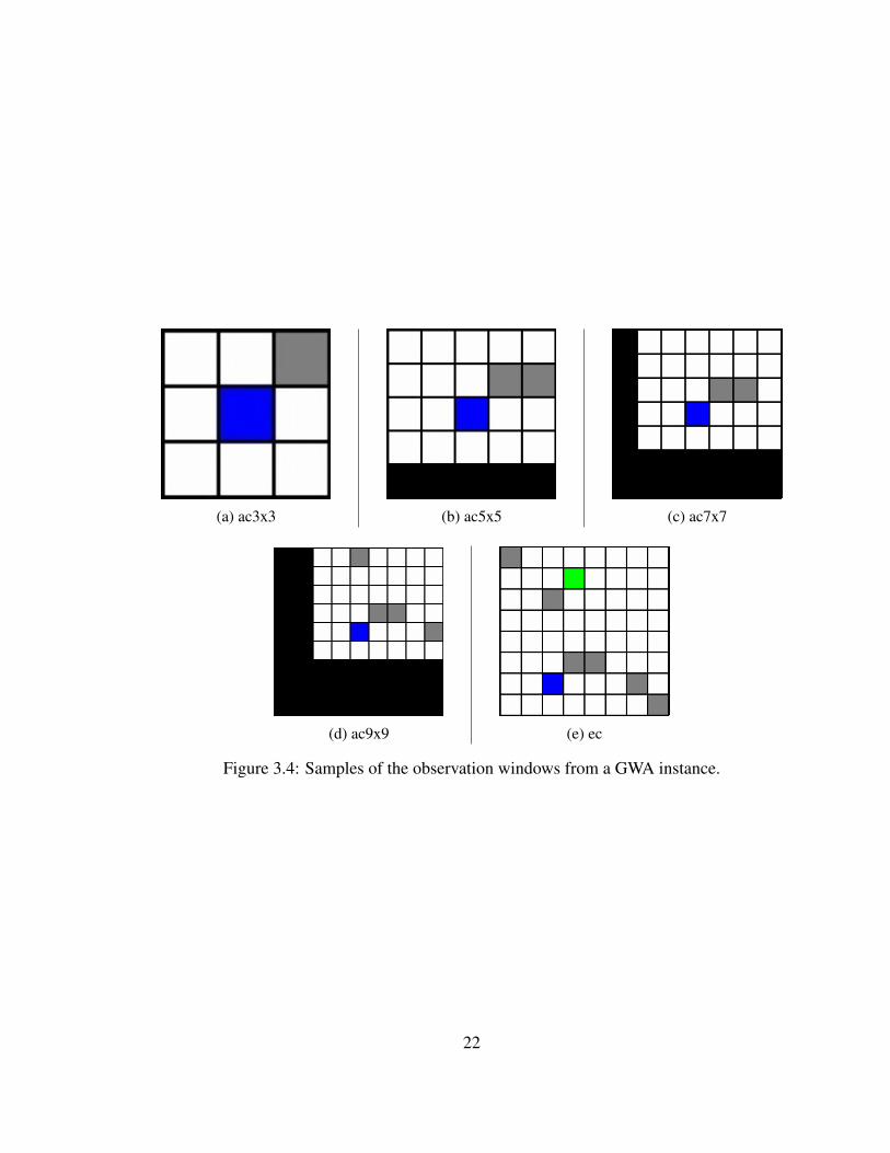
(a) ac3x3 (b) ac5x5 (c) ac7x7

(d) ac9x9 (e) ec

Figure 3.4: Samples of the observation windows from a GWA instance.

22

Chapter 4

Results

4.1 Learning Algorithm & Model Architecture

We evaluated the performance of two learning algorithms (Deep Q-Learning and REIN-

FORCE), four model architectures (1F, 1C1F, 2C1D, and 2C1R), and six meta-tasks (PMT-

GW-A, PMT-GW-B, PMT-GW-C, PMT-GW-D, PMT-GW-E, EPMT-ABCDE) by training

agents with each combination of these features. This resulted in 48 experiments. We re-

port the maximum mean reward over 100 task instances from all evaluation runs for each

PMT algorithm-model-environment trio and EPMT algorithm-model duo in Tables 4.1 and

4.2. We also show policy convergence by reporting the change in mean reward for each

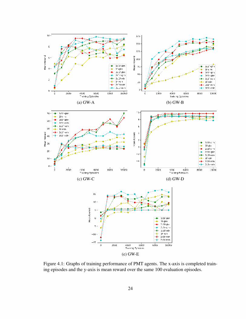
evaluation (every 1000 training episode) for each PMT and EPMT agent in Figures 4.1 and

4.2.

We observe remarkable differences in the results across algorithms, models, and tasks.

Between learning algorithms, REINFORCE performed better on GW-A, GW-C, and GW-D

and Deep Q-Learning performed better on GW-B and GW-E. Between model architectures,

the use of convolutional layers to process the observation before fully-connected or recur-

rent layers significantly quickened convergence towards a good policy, but no significant

23

(a) GW-A (b) GW-B

(c) GW-C (d) GW-D

(e) GW-E

Figure 4.1: Graphs of training performance of PMT agents. The x-axis is completed train-ing episodes and the y-axis is mean reward over the same 100 evaluation episodes.

24

(a) GW-A (b) GW-B

(c) GW-C (d) GW-D

(e) GW-E

Figure 4.2: Graphs of training performance of EPMT agents. The x-axis is completedtraining episodes and the y-axis is mean reward over the same 100 evaluation episodes.

25

Table 4.1: Results of model architecture and learning algorithm over the five ParameterizedMeta Tasks (PMTs)

1f 1c1f 2c1f 2c1rqlrn 6.7 8.4 8.1 9.4rein 8.2 9.4 9.5 9.8

(a) PMT-GW-A


(b) PMT-GW-B


(c) PMT-GW-C


(d) PMT-GW-D


(e) PMT-GW-E

Metric reported is maximum mean reward over 100 task instances from all evaluationruns. The best performers over each PMT are shown in bold.

difference was found between performances of models with recurrent or fully-connected ar-

chitectures. Over the PMT experiments, agents were successfully able to converge towards

the optimal strategy of the presented task and environment except for GW-E, for reasons

which we discuss later in this section. Over the EPMT experiments, the mix of task types

during training resulted in performances worse than PMT, but still generally effective; with

the exception of GW-E which performed significantly better than its PMT counterparts.

The following sections give detailed discussion on agent behavior over the Parame-

terized Meta Tasks and Extended Parameterized Meta Task. The PMT section will give

general characteristics about agent behaviors across the tasks which we will use as a base-

line against the EPMT results. The EPMT section will show agent behavioral gains and

losses as we advance the meta-learning task and discuss the limitations of these agents

under domain generalization.

26

(a) GW-A, qlrn, 2c1r. Stuckin a corner.

(b) GW-A, qlrn, 1c1f. Stuckin a loop.

(c) GW-A, qlrn, 2c1r. Moveson biased action, then towardsvisible goal.

(d) GW-A, rein, 2c1f. Suc-cessfully explores the en-vironment moving counter-clockwise.

(e) GW-A, rein, 2c1f. Stuckin a loop because of walls.

Figure 4.3: Visualizations of PMT-GW-A episodes. The dark blue cell is the agent, andlight blue indicate previously visited cells. Note that the agent’s observation window is 7x7cells centered around the agent.

27

Table 4.2: Results of model architecture and learning algorithm experiment over the Ex-tended Parameterized Meta Task (EPMT-ABCDE)


(a) GW-A


(b) GW-B


(c) GW-C


(d) GW-D


(e) GW-E

Note that a single agent is trained over all tasks composing the EPMT. Metric reported ismaximum mean reward over 100 task instances from each base task from all evaluation

runs. The evaluation task instances are the same as the PMT task instances. The bestresult over each base task is shown in bold.

PMT

GW-A Deep Q-Learning agents tend to bias a single action when no goal object was vis-

ible in the observation window. In many evaluation instances, this resulted in a behavior

where the agent moves towards a corner or edge of the world and stay there until episode

termination (Figure 4.3a). However, when a goal object was within the observation win-

dow, the agent always moved in the direction of the goal (Figure 4.3c). In some instances,

if a wall object blocked the path, the agent was unable to maneuver around it. Wall ob-

jects also tended to have a substantial ”push” effect on the agent’s movement, which led to

circular movement patterns where the agent became ”stuck” when the goal state was not

visible 4.3b. Many of the issues in GW-A Deep Q-Learning agents emerge from a lack

of latent drive for exploration. Q-Learning is effectively a value estimator that measures

exploitability and can only explore when paired with ✏-greedy action selection. However,

this is simply a random action selector, not directed exploration. GW-A REINFORCE

28

agents did not succumb to many of these problematic behaviors because they directly learn

a policy for exploration that uses the edge of the world (which appears as a null vector in

the partially observed, agent-centric observation) as a guide to maneuver the world (Figure

4.3d). Unconstrained by epsilon-greedy action selection and value-estimation, these agents

are capable of effective exploration in the environment. However, even with these capabil-

ities, exploitation-related issues similar to that found in Deep Q-Learning agents continue

to plague the REINFORCE agents. This resulted in a comparable ”push” effect when no

goals were visible in the observation window 4.3e.

GW-B agents are significantly more difficult to characterize than GW-A agents. Perhaps

because of the abundance of goal cells its difficult to observe subtle visual differences in

learned strategies; however, since the difference in reward is apparent in the 1f model,

we are able to make a few observations. The 1f-qlrn agent’s behavior is on par and as

visually complex as the 2c1f-rein model. It is similar to an agent finding and traversing the

shortest path to the nearest goal cell. 1f-rein on the other hand overly favors exploration

and moves around the environment circularly like in the GW-A experiments. It fails to

exploit when given the opportunity. We suspect the heightened performance of the Deep

Q-Learning agents results from a more efficient cluster collection strategy where the agent

stays slightly longer in a corner of the world until all goals respawn in other corners thereby

forming new clusters to exploit.

GW-C agents are particularly sensitive to both the learning algorithm and model archi-

tecture. The low performing GW-C experiments have converged to a policy where it seeks

out the terminal goal, similar to that of the GW-A experiments. If it is convenient (near by

its current position and the trajectory towards the terminal goal), the agent may seek out

non-terminal goals (Figure 4.4a). The degree in which it seeks out non-terminal goals over

terminal goals determines its overall performance. 1c1f-rein most strictly seeks out non-

terminal goals and avoids traps and the terminal goal (Figure 4.4b). rein-2c1r and 2c1r-rein

29

(a) GW-C, qlrn, 1f. Convenience strat-egy.

(b) GW-C, rein, 1c1f. Respawnablegoal consumer, total reward = 125.

Figure 4.4: Visualizations of PMT-GW-C episodes. The dark blue cell is the agent, andlight blue indicate previously visited cells. Note that the agent’s observation window is 7x7cells centered around the agent. The notation ”g-k” and ”t-k” represent the k-th respawn ofa goal cell or trap cell, respectively (0 is the original).

strictly avoid traps, but are somewhat more likely to move towards a terminal goal. All qlrn

agents and the 1f-rein agent tend to collide into traps as it makes its way to the terminal

goal. Interestingly, 1c1f performs best over all the REINFORCE models. A possible ex-

planation is that deeper models create too many abstractions over the positioning of objects

(i.e. the terminal goal’s positioning has dominance in the bias of later representations) and

the 1c1f model provides the necessary amount of complexity needed to process the obser-

vation (unlike 1f) without creating too many abstractions of that observation (unlike 1c1f

or 1c1r).

GW-D has a simpler optimal strategy compared to the other tasks which allowed all

agents to perform well. The low performing agents (all excluding 1c1f-rein and 2c1f-rein)

learned a policy that generally avoided colliding directly with respawnable traps in adjacent

cells. The defining behavior of the well-performing 1c1f-rein and 2c1f-rein agents is to find

and move to an area of the world with fewer traps and maintain position in that ”safer” part

of the world. (Figure 4.5a). All agents acted in such a way to some extent, but the high

performers did so with less error.

30

(a) GW-D, rein, 1c1f. Traparea avoidance.

Figure 4.5: Visualizations of PMT-GW-D episodes. The dark blue cell is the agent, andlight blue indicate previously visited cells. Note that the agent’s observation window is 7x7cells centered around the agent.

(a) GW-E, qlrn, 1c1f. Ex-plores & avoids walls.

(b) GW-E, rein, 1c1f. Center-west bias.

(c) GW-E, rein, 2c1f. Stayingstill.

Figure 4.6: Visualizations of PMT-GW-E episodes. The dark blue cell is the agent, andlight blue indicate previously visited cells. Note that the agent’s observation window is 7x7cells centered around the agent.

31

GW-E agents faced the trickiest task, requiring the algorithm and model to balance

between two optimal strategies – either avoiding movement to gain some positive reward

(maximum of 5 if successful) or seeking out a reward-rich terminal goal while facing move-

ment penalty (maximum of 20 if successful). All Deep Q-Learning agents were able to

succeed to some extent at finding the terminal goal, behaving very similarly to the GW-A

agents. The Q-Learning agents faced the ”push” effects of walls, but also learned how to

explore the environment to find the terminal goal (Figure 4.6a). This behavior may have

emerged from the penalty on collisions and standing still which GW-A Q-Learning agents

did not have to learn. The REINFORCE agents, excluding 1f-rein, were not successful at

finding the terminal goal. The 1f-rein agent performed on par with the lower performing

Q-Learning agents. The 1c1f-rein agent learned a policy that biased movement towards

the center-west cells until it either reached the edge, in which case it stopped movement to

accumulate reward, or found a nearby terminal goal, in which case it moves to consumes it

(Figure 4.6b). The two most complex REINFORCE agents, 2c1f-rein and 2c1r-rein stuck

to the sub-optimal strategy of avoiding movement (Figure 4.6c). The poor performance of

the REINFORCE agents may be a result of the REINFORCE algorithm training the agents

towards the suboptimal strategy, which they are unable to escape from.

EPMT

Of all EPMT agents, the 1c1f-rein agent had the best performance over the GW-A, GW-D,

and GW-E, and good performance over GW-B and GW-C. As a result, we will use it as the

main benchmarking agent to compare against the PMT tasks.

Over the GW-A task instances, the EPMT 1c1f-rein agent performs with near perfect

results, almost always reaching a terminal goal state. However, a striking behavioral issue

is the noisiness of movements leading to substantially longer episodes than in the PMT ex-

periments. This disadvantage does come with the benefit of allowing the agent to overcome

32

”push” effects and stuck states which plagued the PMT agent’s behavior.

Over the GW-B task instances, the EPMT 1c1f-rein agent performs similarly to the

PMT agents: gravitating towards clusters and consuming nearby goal cells; however, like

with GW-A, the agent’s movement is much noisier than the PMT counterparts. As a result,

the shortest path traversal which PMT GW-B agents took now tend to take more steps and

accumulate less reward in an episode.

Over the GW-C and GW-D task instances, the EPMT 1c1f-rein agent performs on par

with the corresponding PMT Deep Q-Learning agents. For GW-C, those agents sought the

terminal reward with some regard for non-terminal rewards if they were on the path to the

terminal reward. For GW-D, those agents generally avoided direct collision with the trap

cells but did not attempt to center themselves in regions with fewer traps.

Over the GW-E task instances, the EPMT 1c1f-rein agent performs significantly better

than the corresponding PMT REINFORCE agents, and performs slightly better than the

best PMT Deep Q-Learning agent. The EPMT agent’s behaviors learned from the GW-A

task is conveniently the better, reward-rich strategy on the GW-E task. The PMT agents are

unable to effectively learn that strategy on their own, but the transference of knowledge to

a new task leads them to it.

EPMT agents generally learned an abstract version of all these tasks that relied solely

on the physical representation of the environment which was shared between each base

task (each similar type of object in each task used the same representation). The nuances

in the strategies that led to more successful performances, especially relating to the reward

structure differences that led to precision in movement for tasks GW-A and GW-B and bet-

ter strategies for tasks GW-C and GW-D were entirely lost in the EPMT agents. However,

the transfer of knowledge between the tasks allowed for a ”lucky” improvement in GW-E

performance.

33

Table 4.3: Results of observation window experiment

ac3x3 ac5x5 ac7x7 ac9x9 ec9.5 8.8 9.5 9.1 7.0

(a) PMT-GW-A

ac3x3 ac5x5 ac7x7 ac9x9 ec106.5 130.2 134.4 126.1 22.5

(b) PMT-GW-B

Metric reported is maximum mean reward over 100 task instances from all evaluationruns.

(a) GW-A (b) GW-B

Figure 4.7: Graphs of training performance of observation window experiment agents. X-axis is training episodes, Y-axis is mean reward over 100 evaluation episodes.

4.2 Observation Window

Of the five observation windows, the ac3x3, ac7x7, and ec windows had the most distinct

performances, so we’ll center discussion around those three windows. We report the maxi-

mum mean reward over 100 task instances from all evaluation runs for each agent in Table

4.3 and show the policy convergence by reporting the change in mean reward for each

evaluation (every 1000 training episodes) in Figure 4.7.

The fully-observed environment-centric observation performed worst on both GW-A

and GW-B with the agent taking on an often chaotic behavior with semi-random actions.

Environment-centric observations are at a disadvantage to agent-centric observations be-

cause they require the agent to interpret their relative position to other objects in the world

within the dynamics of the model. This is not a trivial task for a neural network-based

34

(a) ac7x7 (b) ac7x7 (c) ac9x9

Figure 4.8: Visualizations of GW-A episodes with a 7x7 or 9x9 observation window from2c1f agent.

agent.

The ac5x5, ac7x7, and ac9x9 observations take in the immediate surroundings of the

agent as well as information about objects in the distance. The greater the window size,

the more information the agent could use to make decisions. In GW-A, this often led to

better long term planning, as the agent is able to identify the direction of the terminal

goal (Figure 4.8b). However in some instances, if a wall object blocked the path, the

agent would become blocked by the overpowering force of the goals. Wall objects tend

to have a substantial ”push” effect on the agent’s movement, leading to circular movement

patterns where the agent becomes ”stuck” (Figure 4.8c). Over the GW-B environment, the

observation window provides an effective way to search for and consume clusters of goal

cells. The abundance of reward cells throughout the world reduce the effect of wall ”push”

effects and circular movement patterns.

The ac3x3 observations only take in the immediate surroundings of an agent. Remark-

ably, the agent is able to learn an effective strategy over the GW-A task that is as good as the

ac7x7 agent’s performance, but with radically different behavior. The agent hugs the world

edge or wall objects near the edge to locate itself, while increasing the search space for

environmental exploration of the terminal goal (Figure 4.9c). This is usually an effective

35

(a) (b) (c)

Figure 4.9: Visualizations of GW-A episodes with a 3x3 observation window from 2c1fagent.

way of finding the goal, but in certain situations the agent never found a terminal goal and

became trapped in a loop (Figures 4.8a or 4.8b). Over the GW-B task, the abundance of re-

wards allows it to use the same strategy as GW-A to continually explore and consume goal

cells even as goal cells move around the field. It is not as effective as planning with larger

areas of the field, but it is an effective strategy given the observation space constraints.

36

Chapter 5

Conclusion

An ongoing challenge of meta learning and artificial intelligence is increasing the region

of tasks over which learners can perform. We have formalized a characterization of these

spaces and shown the wide breadth of possible tasks available with Gridworld that are flex-

ible enough to show issues across learning algorithm, model architecture, environmental

observation, and agent design as a whole. This work has sought to use domain general-

ization to expose the limitations of deep-learning based agents on meta learning and we

provide our findings and conclusions below.

We have shown the limitations of deep-learning based agents with different algorithms

and models across multiple Gridworld-based tasks. While generalization across instances

within a task distribution is achievable, generalization across a task region is not simple

under existing methods. The key issue of generalized agents is that they lose knowledge

of important specializations that enable good performance over base tasks. It is likely

that few-shot learning techniques similar to MAML would be effective with an EPMT

agent to specialize it leading to a performance on par or better than a PMT agent [5].

However, there continues to be a missing component within EPMT agents that allows for

dynamic task adaptation when presented with a novel task with different underlying reward

37

structures and task goals. We would expect some form of dynamic task adaptation to work

well in these circumstances if tasks were designed in a few-shot learning fashion, instead

of retraining models where the internal dynamics of the model adapt to the novel task.

This is similar to RL2 and MetaRL which perform well on PMT-like tasks (as presented

in [4, 22] over non-Gridworld environments), but good performance over EPMT-like tasks

with different reward structures remains an open challenge.

Another important lesson from our experiments is the criticality of agent design param-

eters such as observation window, model architecture, and environmental design. The lack

of behaviors on agents with environment-centric observation, the tradeoffs of agent-centric

7x7, and the resilience of ac3x3 agents show the importance of balance between agent de-

sign. Different models and internal agent structures applied to any of these features could

lead to substantially different behavioral results. Deeper neural networks with as many as

five or ten layers have been applied to challenging domains such as the game of Go [13].

Such a network applied to the environment-centric task may allow the agent to properly

gain some spatial perspective leading to good performance, but typically such larger net-

works tend to be difficult to control with learning algorithms like Deep Q-Learning and

REINFORCE. Over the agent-centric 5x5, 7x7, and 9x9 observations, a key improvement

is adding balance between observations of high-reward potential and possible blockers (i.e.

push effect of walls). The convolutional architecture used in many models seems to com-

plement spatial relations that are near (i.e. goal state is adjacent to the agent). Abandoning

the convolutional architecture for a multitude of fully-connected layers tend to result in

catastrophic forgetting during training, especially in a task with high variance in the obser-

vational input as observed in reinforcement learning with Gridworld. This is a significant

deficiency of these approaches and new architectures, perhaps which are general-purpose

and adaptive to novel circumstances, should be considered.

One possible goal in this direction is the development of strategies for the emergence

38

of model-based reinforcement learning behaviors given a model-free context when not pre-

sented with any other knowledge of the domain. Work by others has hinted at the possibility

of using temporal connections through recurrent neural network units [22]. Our results do

not show significant improvements between the fully connected and recurrent networks, so

it is unlikely that any persistent state is formed that is meaningfully used by the model to

improve behavior. The lack of temporal and perhaps model-based characteristics in this ex-

periment do not mean it is not possible; perhaps either a generalization-oriented task design

or neural network-based agent design are insufficient to produce this type of behavior.

39

Bibliography

[1] Gavin Adrian Rummery and Mahesan Niranjan. On-line q-learning using connection-

ist systems. Technical Report 166, Cambridge University Engineering Department,

1994.

[2] Marcin Andrychowicz, Misha Denil, Sergio Gomez Colmenarejo, Matthew W. Hoff-

man, David Pfau, Tom Schaul, and Nando de Freitas. Learning to learn by gradient

descent by gradient descent. In Advances in Neural Information Processing Systems

29, pages 3981–3989. 2016.

[3] Kai Arulkumaran, Marc Peter Deisenroth, Miles Brundage, and Anil Anthony

Bharath. A brief survey of deep reinforcement learning. IEEE Signal Processing

Magazine, 34:26–38, 2017.

[4] Yan Duan, John Schulman, Xi Chen, Peter L. Bartlett, Ilya Sutskever, and Pieter

Abbeel. Rl2: Fast reinforcement learning via slow reinforcement learning, 2016.

arxiv:1611.02779.

[5] Chelsea Finn, Pieter Abbeel, and Sergey Levine. Model-agnostic meta-learning for

fast adaptation of deep networks. In Proceedings of the 34th International Conference

on Machine Learning, pages 1126–1135, 2017.

[6] Abhishek Gupta, Russell Mendonca, YuXuan Liu, Pieter Abbeel, and Sergey Levine.

40

Meta-reinforcement learning of structured exploration strategies. In Advances in Neu-

ral Information Processing Systems 31, pages 5302–5311. 2018.

[7] Matthew Hausknecht and Peter Stone. Deep recurrent q-learning for partially ob-

servable mdps. In Association for the Advancement of Artificial Intelligence Fall

Symposium on Sequential Decision Making for Intelligent Agents, 2015.

[8] Melvin Johnson, Mike Schuster, Quoc V. Le, Maxim Krikun, Yonghui Wu, Zhifeng

Chen, Nikhil Thorat, Fernanda Viegas, Martin Wattenberg, Greg Corrado, Macduff

Hughes, and Jeffrey Dean. Google’s multilingual neural machine translation system:

Enabling zero-shot translation. Transactions of the Association for Computational

Linguistics, 5:339–351, 2017.

[9] Vijaymohan Konda. Actor-critic Algorithms. PhD thesis, Massachusetts Institute of

Technology, 2002.

[10] Yann LeCun, Yoshua Bengio, and Geoffrey Hinton. Deep learning. Nature,

521:436–444, 2015.

[11] Christiane Lemke, Marcin Budka, and Bogdan Gabrys. Metalearning: a survey of

trends and technologies. Artificial Intelligence Review, 44(1):117–130, 2015.

[12] Sergey Levine, Chelsea Finn, Trevor Darrell, and Pieter Abbeel. End-to-end training

of deep visuomotor policies. Journal of Machine Learning Research, 17:1–40, 2016.

[13] Volodymyr Mnih, Koray Kavukcuoglu, David Silver, Andrei A. Rusu, Joel Veness,

Marc G. Bellemare, Alex Graves, Martin Riedmiller, Andreas K. Fidjeland, Georg

Ostrovski, Stig Petersen, Charles Beattie, Amir Sadik, Ioannis Antonoglou, Helen

King, Dharshan Kumaran, Daan Wierstra, Shane Legg, and Demis Hassabis. Human-

level control through deep reinforcement learning. Nature, 518:529–533, 2015.

41

[14] Eleni Nisioti, Kyriakos C. Chatzidimitriou, and Andreas L. Symeonidis. Predicting

hyperparameters from meta-features in binary classification problems. In Proceedings

of the International Workshop on Automatic Machine Learning, 2018.

[15] Marc Ponsen, Matthew E. Taylor, and Karl Tuyls. Abstraction and generalization

in reinforcement learning: A summary and framework. In Proceedings of the 2nd

International Conference on Adaptive and Learning Agents, pages 1–32, 2010.

[16] Esteban Real, Sherry Moore, Andrew Selle, Saurabh Saxena, Yutaka Leon Suematsu,

Quoc V. Le, and Alex Kurakin. Large-scale evolution of image classifiers. In Proceed-

ings of the 34th International Conference on Machine Learning, pages 2902–2911,

2017.

[17] Olga Russakovsky, Jia Deng, Hao Su, Jonathan Krause, Sanjeev Satheesh, Sean Ma,

Zhiheng Huang, Andrej Karpathy, Aditya Khosla, Michael Bernstein, Alexander C.

Berg, and Li Fei-Fei. Imagenet large scale visual recognition challenge. International

Journal of Computer Vision, 115(3):211–252, 2015.

[18] Juergen Schmidhuber, Jieyu Zhao, and Marco Wiering. Simple principles of met-

alearning. Technical Report 77-97, Istituto Dalle Molle di Studi sull’Intelligenza

Artificiale, 1996.

[19] John Schulman, Philipp Moritz, Sergey Levine, Michael Jordan, and Pieter Abbeel.

High-dimensional continuous control using generalized advantage estimation. In Pro-

ceedings of the 4th International Conference on Learning Representations, 2016.

[20] Richard S. Sutton and Andrew G. Barto. Reinforcement Learning - An Introduction.

Adaptive Computation and Machine Learning. MIT Press, 1998.

[21] Ricardo Vilalta and Youssef Drissi. A perspective view and survey of meta-learning.

Artificial Intelligence Review, 18(2):77–95, 2002.

42

[22] Jane X. Wang, Zeb Kurth-Nelson, Dhruva Tirumala, Hubert Soyer, Joel Z. Leibo,

Remi Munos, Charles Blundell, Dharshan Kumaran, and Matthew Botvinick. Learn-

ing to reinforcement learn, 2016. arxiv:1611.05763.

[23] Christopher J. C. H. Watkins and Peter Dayan. Q-learning. Machine Learning, pages

279–292, 1992.

[24] Ronald J. Williams. Simple statistical gradient-following algorithms for connectionist

reinforcement learning. Machine Learning, 8(3):229–256, 1992.

43

characterizing agent behavior under meta reinforcement

Documents