Characterizing Dense Urban Areas from MobilePhone-Call Data: Discovery and Social Dynamics

Marcos R. Vieira 1#, Vanessa Frıas-Martınez ‡, Nuria Oliver ‡ Enrique Frıas-Martınez ‡

# Department of Computer Science, University of California, Riverside, CA – USA‡ Data Mining and User Modeling Group, Telefonica Research, Madrid – Spain

mvieira@cs.ucr.edu {vanessa,nuria,efm}@tid.es

Abstract— The recent adoption of ubiquitous computing tech-nologies (e.g. GPS, WLAN networks) has enabled capturinglarge amounts of spatio-temporal data about human motion.The digital footprints computed from these datasets providecomplementary information for the study of social and humandynamics, with applications ranging from urban planning totransportation and epidemiology. A common problem for allthese applications is the detection of dense areas, i.e. areas whereindividuals concentrate within a specific geographical region andtime period. Nevertheless, the techniques used so far face animportant limitation: they tend to identify as dense areas regionsthat do not respect the natural tessellation of the underlyingspace. In this paper, we propose a novel technique, called DAD-MST, to detect dense areas based on the Maximum Spanning Tree(MST) algorithm applied over the communication antennas of acell phone infrastructure. We evaluate and validate our approachwith a real dataset containing the Call Detail Records (CDR) ofover one million individuals, and apply the methodology to studysocial dynamics in an urban environment.

I. INTRODUCTION

While the mobility of animals has already been quantita-tively studied, e.g. marine predators [1], our understanding ofindividual human mobility is somewhat limited, mostly due tothe lack of large scale quantitative mobility data. However, therecent adoption of ubiquitous computing technologies by verylarge portions of the population (e.g. GPS devices, ubiquitouscellular networks) has enabled the capture of large scalequantitative data about human motion [2], [3], [4]. Some of theareas that directly benefit from this new source of informationare urban computing and smart cities [5], [6]. These areasfocus on improving the quality of life of an urban environmentby understanding the city dynamics through the data providedby ubiquitous technologies.

A city is an inherently self-organized human-driven organi-zation where individuals and their behavior play an importantrole in defining the pulse and the dynamics of the city. Thisimplies that in order to efficiently model human mobility,individual information is necessary in order to reflect thatlocation is, at least in part, each individuals decision [6].The datasets captured by ubiquitous computing technologiesinherently reflect individual information relating to mobilityand social dynamics. This fact represents a huge improvementwhen compared to how mobility data has been typically col-lected: using questionnaires and surveys, and in more advancedstudies, using proxies such as bills, public transport, etc [7].

1Work done while author was an intern at Telefonica Research, Madrid.

Some of the applications of smart cities and the study ofsocial dynamics include traffic forecasting [8], modeling ofthe spread of biological viruses [9], urban and transportationdesign [8] and location-based services [10]. A challenging andinteresting problem related to social and human dynamics isof identifying areas of high density of individuals and theirevolution over time. This information is of paramount impor-tance for, among many others, urban and transport planners,emergency relief and public health officials, as it provides keyinsights on where and when there are areas of high densityof individuals in an urban environment. Urban planners canuse this information to improve the public transport systemby identifying dense areas that are not well covered by thecurrent infrastructure, and determine at which specific timesthe service is more needed. On the other hand, public healthofficials can use the information to identify the geographicalareas in which epidemics can spread faster and, thus, prioritizepreventive and relief plans accordingly.

The problem of dense area detection was initially presentedin the data mining community as the identification of the set(s)of regions, from spatio-temporal data, that satisfy a minimumdensity value. This problem was initially solved for spatialand multidimensional domains [11], and later for spatio-temporal domain [12], [13], [14]. In the former proposals, notime dimension is considered, while in the later ones onlymoving objects, typically represented by GPS sensors thatcontinuously report their locations, are considered. Commonto all of the above methods is that a fixed-size non-overlappinggrid or circle employed to aggregate the values over thespatial dimensions are considered. Therefore, these methods“constrain” the shape of the detected areas and, generally,identify dense areas that are a superset/subset of the desirabledense areas. Ideally, we seek a technique that is able to detectdense areas whose shape is as similar as possible to theunderlying dense geographical areas.

In this paper we propose the Dense Area Discovery(DAD-MST) algorithm to automatically detect dense areasin cell phone networks. Our approach, unlike the previousapproaches, is not based on fixed-size grids, but on thenatural tessellation of the spatial domain, thus overcomingthe limitations of all the previous approaches. The DAD-MSTis especially suited to work with human mobility data fromcell phones. Nevertheless, the type of information used by theDAD-MST is not only available to telecommunication com-panies but also to an increasingly large number of companies

IEEE International Conference on Social Computing / IEEE International Conference on Privacy, Security, Risk and Trust

978-0-7695-4211-9/10 $26.00 © 2010 IEEE

DOI 10.1109/SocialCom.2010.41

241

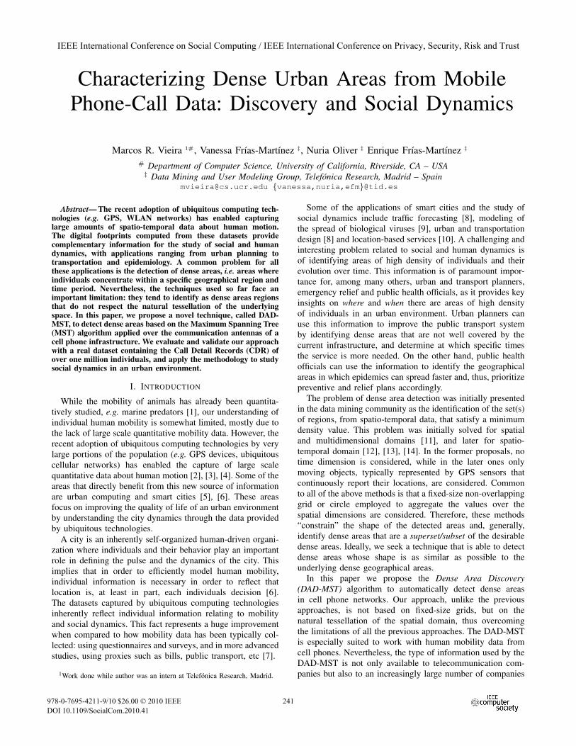
(a) Original Tessellation (b) Desired dense area (c) Grid dense area

Fig. 1. (a) the original tessellation for an urban area, where each polygon defines the coverage of a cell phone tower; (b) the ideal dense area (highlighted)based on the tessellation of the data; (c) common techniques based on fixed-size grids fails on the identification of dense area.

that provide location-based services and mobile services whichalso collect (or are able to collect) human mobility data usingthe cell phone network infrastructure. Moreover, althoughthe DAD-MST algorithm has been designed considering theinfrastructure of a wireless phone network, it can also beapplied to any problem where the data is represented in adomain that has a natural tessellation (e.g. zip codes). Weevaluate the proposed algorithm with a very large, real-worldCall Detail Record (CDR) dataset, and then validate it with astudy of the social dynamics in a urban environment.

Note that the focus of this paper is on the detection andstudy of dense areas, not hotspots [15]. Hotspots, as definedby scan statistics, are the largest discrepancy areas in whichan independent variable has statistically different count valuesfrom the rest of the geographical areas [16]. Conversely,dense areas are defined as the (global or local) maxima ofthe distribution of the function under study [17]. Thus, theinformation provided by both approaches is different, whilehotspots can be used to identify events, dense areas identifyregions in space with a minimum critical mass of individuals.

The remainder of this paper is organized as follows: SectionII discusses the related work; Section III formally defines theproblem of discovering dense areas; Section IV describes theproposed approach and its evaluation and validation appear inSection V; A case study of the dynamics of a city from adense area perspective is described in Section VI; and SectionVII concludes the paper.

II. RELATED WORK

In the GIS, Urban Planning, Transportation and VirusSpreading communities there has been (for a long time) avariety of models to study human and city dynamics. Tradi-tional approaches divide the geographical region under studyin zones which exchange population among themselves. Eachzone is characterized by a vector of socio-economic indicators[5], typically collected and generated using surveys. Also, thisinformation can be completed with proxy sources for humanmobility such as transport infrastructures, air connections, etc[7], [9]. These approaches provide information about humanbehavior in a geographical environment but they are verydifficult to update and limit the results to a moment in

time [18]. In any case, these models substitute humans withderivatives of their activities, ignoring the self-driven natureof human mobility. The use of data originating in pervasiveinfrastructures captures each individual mobility and is ideal torepresent the self-driven nature of the problem, complementingtraditional approaches. In [18], [19], the authors discuss initialguidelines on how mobile phone data can be relevant for urbanplanning and transportation communities.

Previous works on the identification of dense areas, notnecessarily for the study of social dynamics, have been car-ried out following three main approaches: (1) density-basedclustering techniques; (2) detecting dense fixed-size grids inspatio-temporal data; and (3) spatial-based techniques to detectlocal maxima areas.

Clustering algorithms for spatial, multidimensional andspatio-temporal data have been the focus of a variety ofstudies (e.g. [20], [21], [22], [23]). Common to all of theabove methods is that clusters with high numbers of objectsin a specific geographical area are associated, using spatialproperties of the data, to denser regions. Furthermore, allof these methods require choosing some number of clustersor making underlying distributional assumptions of the data,which is not always easy to estimate.

There are a variety of solutions for detecting dense areasin spatial [11] and spatio-temporal [12], [13], [14] domains.The STING method [11] is a fixed-size grid-based approach togenerate hierarchical statistical information from spatial data.Hadjieleftheriou et al. [14] present another method based onfixed-size grids where the main goal is to detect areas witha number of trajectories higher than a predefined threshold.Algorithms using a fixed-size window are proposed in [12],[13] to scan the spatial domain in order to find fixed-size denseregions. All of these approaches are specifically designed towork for trajectory data where the exact location and speeddirection of a trajectory are used in order to aggregate valuesin each grid for the spatial domain. Unfortunately, thesemethods cannot be applied to our domain since in the majorityof mobile phone databases mobile users are not continuoustracked. Furthermore, all the works described here detect denseareas of fixed-size above a threshold using a predefined grid.

Some solutions to detect dense areas are based on the iden-

242

tification of local maxima, typically using techniques inheritedfrom computer vision (e.g. mean-shift [16], [15]). Mean shiftis a non-parametric feature-space analysis technique that iden-tifies the modes of a density function given a discrete datasetsampled from that function. As in previous approaches, thegeographical space under study is divided into a grid, henceignoring other original (natural) tessellations. Crandall et al.[17] use mean-shift to identify geographical landmarks fromgeo-tagged images.

In summary, previous works, among other limitations, typ-ically identifies dense areas by overlaying a fixed grid on thegeographical region, which might not correspond to the realshape of the underlying dense area. Although this problemcan be tackled to some extent with the creation of a gridwith enough granularity to linearly approximate the naturaltessellation of the area under study, the exponential increasein complexity makes this solution computationally unfeasible.

III. PRELIMINARIES

In order to study the social dynamics of a geographical area,we propose a new technique to identify dense areas and studytheir evolution over time using the ubiquitous infrastructureprovided by a cell phone network. Cell phone networks arebuilt using a set of cell towers, also called Base TransceiverStations (BTS), that are in charge of communicating cellphones with the network. Each BTS has a latitude and alongitude, indicating its location, and gives cellular coverage toan area called a cell. We assume that the cell of each BTS is a2-dimensional non-overlapping polygon, and we use a Voronoitessellation to define its coverage area. Neighboring towers canthus be identified using the Delaunay triangulation. Ideally, analgorithm to detect dense areas in this context should respectthe tessellation produced by the Voronoi.

An example of the problems that arise when using the tradi-tional techniques presented in the previous section is illustratedin Figure 1: Figure 1(a) depicts the natural tessellation of acity given by cell towers, with each polygon representing itscoverage; Figure 1(b) highlights the desired dense area (inthis case an area of high mobile-phone activity) based on theoriginal tessellation; and Figure 1(c) represents the dense areaidentified by a state-of-the-art grid technique (with cell sizesimilar to the size of the cells in the tessellation). Note that inthe latter case, the dense area found by the algorithm includesgeographical regions with low density of activity (e.g. parks)due to the grid structure employed. Moreover, due to the natureof the grid structure, a larger area than what it is in reality isreturned by the grid-based algorithms.

Call Detailed Record (CDR) databases are populated when-ever a mobile phone makes/receives a phone call or uses aservice (e.g. SMS, MMS). Hence, there is an entry in the CDRdatabase for each phone call/SMS/MMS sent/received, with itsassociated timestamp and the BTS that handled it, which givesan indication of the geographical location of the mobile phoneat a given moment in time. Note that no information about theposition of a user within a cell is known.

We characterize the information handled by each BTS oftwo types: activities and users. The activities, A(δt)i, at btsi

correspond to the number of different calls that were handledby btsi during the time period δt. Likewise, U (δt)i measuresthe number of unique individuals whose calls where handledby btsi during the time period δt.

In order to study the social dynamics of a region usingcell phone networks, we propose the DAD-MST algorithmto automatically discover dense areas of activities or uniqueusers in a specific geographical region and during a determinedperiod of time δt such that: (1) it respects the originaltessellation of the space defined by the cell phone network;(2) it does not need as input the number of dense areas (e.g.the number of clusters) to be identified; and (3) it guaranteesthat all dense areas are identified, covering up to a maximumpercentage λ of the total region under consideration. In ourscenario, the geographical region corresponds to the total areawhere the dense spots are to be identified, and we carry outour analysis at three levels: urban, regional and national.

IV. DISCOVERING DENSE AREAS FROM CDR DATA

Given an initial set of BTS={bts1,bts2, ...,btsn} that givescoverage to a geographical region R characterized by itsVoronoi tessellation R = {V1 ∪ V2 ∪ ... ∪ Vn}, we seek todiscover the optimal disjoint subsets of BTS that cover areaswithin R where either the number of activities or unique usersreaches a maximum in a specific time period δt. An exhaustiveexploration of all possible disjoint subsets of BTS becomesa daunting task as the number of BTS increases. Thus, wepropose a greedy algorithm based on the Maximum SpanningTree (MST) algorithm [24] that selects, at each step, the bestsubsets of BTS. In order to smooth noisy data, the minimumnumber of BTS that define a dense area is set to 2.

The algorithm computes the dense areas in a geographicalregion R given two parameters: coverage λ and granularityξ. The coverage λ corresponds to the maximum percentageof the geographical area R that can be covered by the denseareas identified by the algorithm. Typical values for λ are inthe range 0.05 to 0.5 (5% and 50%, respectively). Smaller λvalues may risk not identifying dense areas, and larger valuesare considered not relevant as the areas identified would covermost of the region R under study.

The granularity ξ represents the maximum distance betweentwo BTS in order to consider them to be part of the same densearea and to be joined to form a potential subset. Hence, theparameter ξ sets the spatial granularity at which dense areasare identified (e.g. urban, regional or national levels) and itis similar to the scale of observation parameters employed inthe mean-shift approach in [17]. When seeking an adequatevalue for ξ, the distribution of BTS is a key factor. In urbanareas this distribution is typically very dense and homogeneoussuch that each cell covers similar extension of areas. However,in sparsely populated areas (e.g. rural area), the distributionof BTS is scarce. For example, the average distance betweentwo neighboring urban BTS is around 1km, while in ruralenvironments this value may increase up to 11km. Therefore,suitable values for ξ could be 1km, 10km and 100km to detectdense areas in urban, regional, and national level, respectively.

243

The proposed Dense Area Discovery via MST algorithm(DAD-MST) consists of three phases (explained below): (A)Graph Construction; (B) Computation of Dense Areas; and (C)Post-processing. It receives as inputs: the geographical regionR, the time period δt for which the dense areas need to becomputed, the set of BTS in the region R, the coverage λ andthe granularity ξ. It generates as outputs the subsets of BTSthat correspond to the dense areas in region R with coverageλ and granularity ξ.

A. Graph ConstructionFirst, a graph G=(V ,E) is built using Delaunay triangula-

tion, where each vertex vi ∈ V corresponds to btsi ∈ BTS inthe geographical region R, and each edge ei,j ∈ E representsthe connection between btsi and btsj . The Delaunay trian-gulation is implemented following the Divide and Conquerapproach [25], with an approximate complexity of O(V logV ).Next, all the edges in E with a distance between the twoconnecting BTS larger than ξ are eliminated from the graph,in order to ensure the desired spatial granularity given by ξ.The distance between two BTS is computed by translatingtheir geographical coordinates into Cartesian coordinates andthen computing their Euclidean distance.

After that, a weight wi,j is associated to each edge ei,j ∈E that has not been eliminated. The weight represents theaverage density of the area covered by btsi and btsj duringthe time period δt. The density is given by two types: the totalactivity (A(δt)i+A(δt)j) or the total number of (unique) users(U (δt)i+U (δt)j) observed at btsi and btsj during δt, divided bythe geographical area (in km2) covered by btsi and btsj . Bothvalues are computed from the CDR database using a querysystem (see subsection CDR Query System). The details ofthe algorithm are presented in Algorithm 1.

Algorithm 1 GraphConstruction(type,BTS,ξ,δt)1: G(V,E)← Delaunay(bts1, ...,btsn)2: for each edge ei,j ∈ E do3: if distance(btsi,btsj) > ξ then4: E ← E \ ei,j

5: else6: wi,j ← QueryDB(type,btsi,btsj ,δt)

B. Computation of Dense AreasA variation of the Maximum Spanning Tree algorithm is

used to detect dense areas given by G(V ,E) and the associatedweights W (see Algorithm 2). The edges in E are first sortedby decreasing weight W . At each step the edge ei,j ∈ Ewith the highest weight wi,j is removed from E and addedto the list L of edges that represent dense areas if and only ifthe edge connects vertices that belong to two different subsets(trees) of BTS. In Algorithm 2, MakeSet creates a potentialtree for each vertex, FindSet identifies the tree in which avertex is included in L, and Union joins two trees. A detaileddescription of MakeSet, FindSet and Union is given in theformal definition of the MST algorithm [24].

This process selects, in a greedy manner, the subsets ofvertices (BTS) that are associated to high values of either

activities or unique users. Edges are added to L until the totalgeographic area covered by the BTS that are connected by theedges in L is equal or larger than λ ∗ |R|, where λ is thecoverage and |R| is the size of the area under study. Notethat the coverage of btsi is approximated by the area of itsassociated Voronoi cell Voronoi(btsi), such that the algorithmcomputes the tree until

∑Voronoi(btsi) ∀i ∈ unique btsi of

|L| > λ ∗ |R|. Additionally, every time an edge ei,j is addedto L, the edges in E where either i or j are one of the vertices,are re-weighted in order to avoid double counting of activitiesor unique users. Once the stopping condition is satisfied, thelist L contains all the edges (and associated pairs of BTS) thatcorrespond to the dense areas in the graph. The complexity ofComputeDenseAreas is O(ElogE).

Algorithm 2 ComputeDenseAreas(G(V,E),R,λ)1: sort E by decreasing weight W2: L← ∅3: for each vi ∈ V do4: MakeSet(vi)5: while

∑Voronoi(btsi) ∀i ∈ unique btsi of |L| < λ ∗ |R| do

6: ei,j ← E.top()7: E ← E \ ei,j

8: if FindSet(i) 6= FindSet(j) then9: L← L

⋃ei,j

10: Union(i, j)11: re-weight ∀ei′,j′ ∈ E affected by ei,j

12: sort E by decreasing weight W

C. Post-processing

The post-processing phase computes all the connected com-ponents from the final list L in order to visualize the denseareas on a map. Each subset of connected edges in L representsa subset of BTS associated to a dense area. Specifically, we usethe Shiloach-Vishkin [26] algorithm to compute the connectedcomponents of the graph (with a complexity of O(ElogV )).Once the connected edges are obtained, the final density ofactivities or unique users associated to each dense area arecomputed as the sum of the weights of all of its edges dividedby the geographical area (in km2) covered by all the BTS inthe dense area. Finally, a color is assigned to each dense area(subset of BTS based on its level of activities or users: warm(red, orange, ...) and cold (blue, grey, ...) colors are used torepresent areas with high and low, respectively, dense levels.

D. CDR Query System

The most computationally expensive part of the proposedalgorithm is the calculation of the weights W associated tothe edges E. Since processing a very large CDR databasecontaining several millions of records for a specific period oftime δt can be computationally expensive (especially whenlong periods of time are considered), in this work we makeuse of a spatio-temporal query system designed specificallyfor CDR databases [4] that guarantees a timely retrieval ofinformation associated to any BTS. Basically, for each btsi,two index structures are built: one B+-tree to organize entriesby the temporal attribute timestamp; and one inverted-index

244

where entries are ordered by (phoneid,timestamp). This index-based structure allows us to compute the weights of the edgesby querying the system with the time period δt, the btsi andbtsj , and the type of query (activities/users) under study.

V. EXPERIMENTAL EVALUATION

We collected cell phone data in the form of CDR from asingle carrier of a state with an approximate area of 80,000km2. The state contains two large metropolitan areas (ofapproximately 4,000,000 and 400,000 residents respectively)and other smaller urban areas. Here we use a sample of thisdataset containing the calls of over one million anonymizedunique customers over a period of four months, with around50 million CDR entries collected with 5,000 BTS towers2.

A. Quantitative Evaluation

First, we experimentally analyze the effect that ξ (granu-larity) and λ (coverage) have in the number of dense areasidentified and by extension in the granularity of the socialdynamics modelled. For that purpose, we consider two dif-ferent settings for the geographical region R: urban, Ru,defined by a rectangle (Ru=30km*35km) that covers the mainmetropolitan area (4, 000, 000 residents); and regional, Rr,defined by a rectangle (Rr=400km*200km) that approximatelycovers all the geographical area of the state. Regarding thetemporal range δt, we consider “weekdays” and “weekends”separately and within each type of day, we identify four timeslots: “mornings” (6am–10am), “afternoons” (10am–2pm),“evenings” (2pm–6pm) and “nights” (6pm–10pm). Note thatwe present here results for δt=“weekdays in the morning” andfor the type of query number of users due to space constraints,but we obtained similar results with the other temporal rangesand the number of activities.

Figure 2 (top) shows the number of dense areas (Y axis)obtained by the DAD-MST algorithm with different values ofcoverage λ from 5% to 50% (X axis) for the urban geograph-ical region Ru=30km*35km. Each line in the plot represents adifferent value for ξ: 1km (urban), 10km (regional) and 100km(national). Considering ξ=1km, we observe that as λ increases,the number of dense areas identified by the algorithm increaseslinearly. The algorithm successfully identifies different denseareas due to the fact that ξ=1km does not allow for many BTSconnected by Delaunay to be merged together as the area ofcoverage increases. However, we observe that for larger valuesof ξ, the increase in coverage results in a reduction in thenumber of dense areas. This is due to the fact that larger ξsmerge dense areas together as the coverage area is increased.In fact, we observe that for ξ=10km and ξ=100km, when thearea of coverage is larger than 10%, only one dense area isidentified as all of the edge subsets are joined. In sum, thisanalysis highlights the importance of selecting an appropriatevalue for ξ that will adequately identify areas within the regionunder study. In the case of an urban environment, the valueof ξ=1km successfully achieves this result.

2Company policy does not allow us to reveal the geographical origin of thedata.

Fig. 2. Total number of dense areas identified (Y axis) for values of λ (Xaxis) ranging from 5% to 50% and for ξ=1, 10, 100km. R represents an urban(top) and a regional (bottom - with Y in log scale) area.

Figure 2 (bottom) shows a similar analysis for a regionalgeographical area Rr=400km*200km (Y axis in log scale).In this case, ξ=1km generates a large number of dense areasof small size as the coverage area λ increases. In fact, weare capturing the dense areas within the neighborhoods ofmetropolitan areas located in the region under study. Highervalues of ξ allow us to merge and thus reduce the numberof dense areas identified as λ increases. We observe thatξ=10km stabilizes after identifying approximately 200 denseareas, which correspond to small suburban areas (generallynear metropolitan areas) and/or big neighborhoods withinmetropolitan areas. Finally, for ξ=100km, we observe thatvalues of λ higher that 20% only allow for the detection oftwo dense areas that correspond to the two big metropolitanareas in the region.

Hence, a value of ξ=100km yields the identification of bigmetropolitan areas whereas ξ=10km leads to detecting smallsuburban areas within the region under study. From a com-putational efficiency perspective, the scale of the experimentdeeply affect the computation time. At an urban scale Ru, areduced number of BTS is analyzed (around 500), yielding aprocessing time of less than 30 seconds per evaluation tuple(λ, ξ). At a regional scale Rr, the number of BTS is one orderof magnitude larger (around 5,000). Hence, the processingtime is of the order of 30 minutes per evaluation tuple. Allexperiments were run on a Dual Intel Xeon E5540 2.53GHzrunning Linux 2.6.22 with 32GBytes memory.

B. Qualitative Validation

In order to assess the quality of the areas identified by theproposed algorithm, Figure 3 shows some landmarks of thecity under study, having as a reference the subway system.

245

Fig. 3. General description of the city under study with the subway systemas the main reference landmark.

The two subway lines in the city (represented by dotted-black lines), run East-West (L1) and North-South (L2) withone central station in common. For reference purposes thecentral station is denoted by C, with stops north of C denotedas N1 to N7, stops south of C denoted S1 to S11 andstops east of C denoted E1 to E9. The downtown area isgeographically located around C, E1, E2, E3 and E4. NearC we find university buildings, government offices and parks.The vicinities of E1 and E2 form the commercial part of thecity with markets, commercial streets and hotels. E3 and E4have more university buildings and night life area. The rest ofL1 services mainly residential areas. Regarding L2, around S3to S11 there are mainly residential neighborhoods with lightindustrial areas. N2 to N7 serve residential areas with somecommercial and entertainment places. The map also indicatesother places such as a Stadium complex (S) and the city Zoo(Z), the main zoo of the country. For the areas not commented,as a general rule, there is a mixture of residential areas (withdifferent densities) and light industrial areas, with the northand north-west having more affluent areas than the south.

Figures 4 and 5 depict the graphical representation of thedense areas detected at an urban level (Ru=30km*35km,ξ=1km, λ=15%) during mornings, afternoons, evenings andnights in term of number of users for weekdays and weekendsrespectively. R covers the city and its metropolitan area as toreflect the social dynamics between the metropolitan belt andthe city. The area presented in the figures is a smaller rectangleof 20km*15km centered in the city in order to appreciatedowntown dense areas. Note that the same color in differenttime frameworks does not imply the same density, just thesame relative importance.

The dense areas identified by DAD-MST align well withthe two subway lines, highlighting the intricate relationship be-tween public transportation and city dynamics. This alignment

is also an indirect validation of our algorithm, as it is expectedthat people will concentrate around the areas served by thepublic transport system. Finally, we repeated the analysis forthe variable number of activities with similar results.

VI. CITY DYNAMICS

The combination of Figures 4 and 5 shows the evolutionof dense areas during weekdays and weekends and thus anindication of how people live and move in the city. It has tobe noted that the dynamics reflected by the evolution of denseareas does not necessarily imply flocks of individuals [27]moving from one area to another, just density of individualschanging over time. The top five dense areas presented in eachmap of Figures 4 and 5 have been numbered from 1 to 5 (beingdense area #1 the one with the highest density) to facilitatethe reading of the relevance3. If one number is not present isbecause it is not located in the area of 20km*15km showed inthe Figures 4 and 5 but is present somewhere in R, i.e. in thosecases the dense areas are located outside the city somewherein the metropolitan belt.

Following the temporal sequence of the evolution of denseareas during weekdays (see Figure 4) it can be observed thatdowntown is covered by a big dense area in the morning,focussing on the university, the commercial and the govern-mental district. Also in the morning, the second and fifth denseareas are located in residential zones and dense areas #3 and#4 are outside the city. This indicates that in those hoursalthough downtown is the top dense area, the metropolitanbelt of the city also has important density of individuals. Inthe afternoon, the top dense area that appeared in the morningdisappears, and a new dense area, ranked #2, located aroundE1 to E4 and focussing on the commercial area appears. Alsoin the afternoon, 3 out of the top 5 dense areas identified arein the metropolitan belt. Note that because of the nature ofthe data, we are strictly representing the number of peoplethat have used their cell phone in that period of time. It canbe the case that once people get to the working place or tothe university in downtown, cell phones are not used withthe same frequency. This would motivate the disappearanceof the dense area in the government and university districts.On weekday evenings and nights the activity is concentratedin downtown, with the top dense area around the commercialand business districts and aligning with the subway lines. Bothin the evening and at night there is a shift, when compared tomornings and afternoons, in the localization of the top denseareas from the metropolitan belt to downtown. To representthat shift, in the evening 4 out of the 5 top dense areas are inthe city, while at night the 3 top ones are in the city.

Following the temporal sequence of the evolution of denseareas during weekends (see Figure 5) it can be observed thatin the morning and in the afternoon the top dense area (#1)is outside the city. In both cases there are dense areas inthe commercial and business districts in downtown, althoughthey are not in the top 3. Two dense areas appear north ofdowntown, which include the stadium complex (marked with

3We have ranked the dense areas because the color scheme used in ourgraphic interface does not translate into interpretable grey levels.

246

(a) weekday morning (b) weekday afternoon

(c) weekday evening (d) weekday night

Fig. 4. Area of 20km*15km of the city under study and the dense areas detected by DAD-MST in the morning, afternoon, evening and night during weekdayswith ξ=1km and λ=.15. The black line with black dots represents the subway system and the corresponding stations.

(a) weekend morning (b) weekend afternoon

(c) weekend evening (d) weekend night

Fig. 5. Area of 20km*15km of the city under study and the dense areas detected by DAD-MST in the the morning, afternoon, evening and night duringweekends with ξ=1km and λ=.15.The black line with black dots represents the subway system and the corresponding stations.

247

S) and the zoo (marked with Z) respectively. Both dense areasare present in the four range hours during weekends (notethat both complexes cover a small geographical area of thedense areas identified). During the evenings and at night thetop dense area is in downtown around the subway stops E1 toE4, i.e. in the commercial and nigh life area. Both evening andnights during weekends have the same dense areas, indicatingthat there is no change in the dynamics of the city. As ithappened during weekdays, in the evening and at night thereis a shift in the top dense areas from the metropolitan belt tothe city.

Both during weekdays and weekends residential areas areidentified south of downtown. The identification of dense areasin residential neighborhoods is tightly related to the densityof housing, where lower income neighborhoods tend to havea higher density than more affluent neighborhoods. This isprobably one of the reasons why residential dense areas areidentified mainly in the south and none in the north.

A direct application of these knowledge regarding the socialdynamics of the city is to help in the decision process ofthe design of the public transport infrastructure. In general,as mentioned in the previous section, there is an alignmentbetween the subway lines (especially N1-N11 and E1 to E7)and the dense areas, indicating that the main dense areas arecovered. The dense areas of the south-west are not directlycovered by S1-S11, although they are in the vicinity. Notethat our algorithm has also identified dense areas in the south-east corner of the city, where there is no subway service rightnow. From an urban planning perspective, this informationcould be used to propose line extensions to public transportofficials. Also it is relevant that dense areas are very relevantin the metropolitan belt, and typically in the top 5 mostimportant ones, so enough means of communication (buses,trains, etc.) have to communicate those areas with the city,specially between afternoon and evening when dense areasshift from the metropolitan belt to the city.

VII. CONCLUSION AND FUTURE WORK

Ubiquitous computing infrastructures are opening new doorsfor the study of social dynamics, specially in the field of urbancomputing. The application of these new techniques can beused as a complement to traditional approaches in areas suchas urban planning and transportation design. The identificationof dense areas is a topic that is key to a variety of socialdynamic studies, and as such has received attention from avariety of research fields. Nevertheless, the techniques used sofar suffer from limitations – particularly when using large scalehuman activity data sets, such as mobile phone-call records –including poor spatial resolution due to the use of grids. In thispaper, we have proposed the DAD-MST algorithm to identifydense areas from Call Detail Records that is able to processlarge scale datasets and respects the original tessellation ofthe space. The The DAD-MST algorithm has been tested andvalidated using a real CDR dataset of almost 50 million entriesfor over 1 million unique users over a four-month period. Thedense areas identified have been qualitatively validated usingthe subway system of the city under study. The dynamics of

the dense areas identified revealed the use that the citizensmake of their city, indicating differences between differenthour ranges and weekdays and weekends. We consider thatalthough the results presented can only be applied to the cityunder study, the framework can be generalized to study socialdynamics not only at an urban level, but also at a regionaland national levels using the proper parameters of the DAD-MST algorithm. As future work we plan to combine ourtechnique with data originating from other urban sensors, suchas traffic, and analyze the applicability of our work for therecommendation of urban planning decisions.

REFERENCES

[1] D. Sims and et al., “Scaling laws of marine predator search behaviour,”Nature, vol. 451, 2008.

[2] M. C. Gonzalez, C. A. Hidalgo, and A.-L. Barabasi, “Understandingindividual human mobility patterns,” Nature, vol. 453, 2008.

[3] N. Eagle, Y.-A. de Montjoye, and L. Bettencourt, “Community comput-ing: Comparisons between rural and urban societies using mobile phonedata,” in SocialCom, 2009.

[4] M. Vieira, E. Frias-Martinez, P. Bakalov, V. Frias-Martinez, andV. Tsotras, “Querying Spatio-Temporal Patterns in Mobile Phone-CallDatabases,” IEEE Mobile Data Management Conf., 2010.

[5] I. Benenson, “Modeling population dynamics in the city: from a regionalto a multi-agent approach,” Discrete Dynamics in Nat. and Soc., 1999.

[6] I. Benenson and E. Hatna, “Human choice behavior makes city dynamicsrobust and, thus, predictable,” in GeoComputation, 2003.

[7] D. Brockmann, L. Hufnagel, and T. Geisel, “The scaling laws of humantravel,” Nature, vol. 439, 2006.

[8] L. Liao, D. J. Patterson, D. Fox, and H. Kautz, “Learning and inferringtransportation routines,” Artificial Intelligence, vol. 171, 2007.

[9] D. Brockmann, “Human mobility and spatial disease dynamics,” Reviewof Nonlinear Dynamics and Complexity - Wiley, 2009.

[10] J. Schiller and A. Voisard, Location-Based Services. Morgan Kaufmann,2004.

[11] W. Wang and R. Muntz, “Sting: A statistical information grid approachto spatial data mining,” in VLDB Conf., 1997.

[12] J. Ni and C. Ravishankar, “Pointwise-dense region queries in spatio-temporal databases,” in ICDE, 2007.

[13] C. Jensen, D. Lin, B. C. Ooi, and R. Zhang, “Effective density querieson continuously moving objects,” in ICDE, 2006.

[14] M. Hadjieleftheriou, G. Kollios, D. Gunopulos, and V. Tsotras, “On-linediscovery of dense areas in spatio-temporal databases,” in SSTD, 2003.

[15] D. Agarwal, A. McGregor, J. Phillips, S. Venkatasubramanian, andZ. Zhu, “Spatial scan statistics: Approximations and performance study,”in ACM SIGKDD, 2006.

[16] M. Kulldorff, “A spatial scan statistic,” Communications in Statistics-Theory and methods, 1997.

[17] D. J. Crandall, L. Backstrom, D. Huttenlocher, and J. Kleinberg,“Mapping the world’s photos,” in WWW Conf., 2009.

[18] J. Reades, F. Calabrese, A. Sevtsuk, and C. Ratti, “Cellular census:Explorations in urban data collection,” Pervasive Computing, 2007.

[19] C. Ratti, S. Williams, D. Frenchman, and R. M. Pulselli, “Mobilelandscapes: using location data from cell phones for urban analysis,”Environment and Planning B: Planning and Design, 2006.

[20] M. Ester, H.-P. Kriegel, J. Sander, and X. Xu, “A local-density basedspatial clustering algorithm with noise,” in ACM SIGKDD, 1996.

[21] T. Zhang, R. Ramakrishnan, and M. Livny, “Birch: An efficient dataclustering method for very large databases,” in SIGMOD Conf., 1996.

[22] P. Kalnis, N. Mamoulis, and S. Bakiras, “On discovering moving clustersin spatio-temporal data,” in SSTD, 2005, pp. 364–381.

[23] J.-G. Lee, J. Han, and K.-Y. Whang, “Trajectory clustering: a partition-and-group framework,” in SIGMOD Conf., 2007.

[24] J. B. Kruskal, “On the shortest spanning subtree of a graph and thetraveling salesman problem,” Proc. of the American Math. Soc., 1956.

[25] L. Guibas and J. Stolfi, “Primitives for the manipulation of generalsubdivisions and the computation of Voronoi,” Trans. on Graphics, 1985.

[26] Y. Shiloach and U. Vishkin, “An O(log n) parallel connectivity algo-rithm,” Journal of Algorithms, vol. 3, 1982.

[27] M. Vieira, P. Bakalov, and V. Tsotras, “On-line discovery of flockpatterns in spatio-temporal data,” in ACM SIGSPATIAL Conf., 2009.

248