Clemson UniversityTigerPrints

All Theses Theses

12-2009

Charging Kinetics of Electric Double LayerCapacitorsClint CagleClemson University, ccagle@clemson.edu

Follow this and additional works at: https://tigerprints.clemson.edu/all_theses

Part of the Engineering Mechanics Commons

This Thesis is brought to you for free and open access by the Theses at TigerPrints. It has been accepted for inclusion in All Theses by an authorizedadministrator of TigerPrints. For more information, please contact kokeefe@clemson.edu.

Recommended CitationCagle, Clint, "Charging Kinetics of Electric Double Layer Capacitors" (2009). All Theses. 716.https://tigerprints.clemson.edu/all_theses/716

Charging Kinetics of Electric Double Layer Capacitors

A Thesis

Presented to

the Graduate School of

Clemson University

In Partial Fulfillment

of the Requirements for the Degree

Master of Science

Mechanical Engineering

by

Clint William Cagle

December 2009

Accepted by:

Dr. Rui Qiao, Committee Chair

Dr. Ardalan Vahidi

Dr. Gang Li

Abstract

A recent increase in the popularity of EDLCs and AC-EOF has necessitated a deeper

understanding of the structure and charging kinetics of electrical double layers (EDLs) at

electrode-electrolyte interfaces. Here, the charging kinetics of EDLs in nanoscale EDLCs

is studied by a circuit model, a Poisson-Nernst-Planck (PNP) model, and molecular dy-

namics (MD) simulations. The results of the MD simulations demonstrate a linear charging

behavior of EDLs near planar electrodes for both aqueous and organic electrolytes at charg-

ing below 90% and time larger than tens of picoseconds. Additionally, we will show that

the circuit and PNP models are capable of accurately capturing this linearity, as well as

the overall charging kinetics. Through PNP and MD simulation, a diffusional process is

shown to occur which causes a decrease in the concentration of the bulk solution, yet the

linearity of charging, at charging below 90%, is not be affected because the flux during

the charging process is found to be relatively low. The charging kinetics of a slit nanopore

electrode is also studied using MD, and interesting results about the linearity of this process

is discussed. Finally, a porous geometry modeled by an exohedral pore with multiple solid

cylinders will demonstrate that variations in the surface charge density around the solid

cylinders will occur during charging due to interactions between nearby charged cylinders.

However, these variations in surface charge density along the circumference of the cylinder

will approach zero as the system reaches equilibrium.

ii

Dedication

I dedicate the following thesis to my family and my future wife Brooke.

iii

Acknowledgments

I would like to thank my adviser Dr. Qiao for his relentless push for excellence out

of me, and for his desire to see me and this thesis succeed. Also, I would like to thank

Quang and Ping for all their help over the past two years, and also CCIT and the people

behind Palmetto Cluster. Lastly, I thank Brooke and my family for their love and support.

iv

Table of Contents

Title Page . . . . . . . . . . . . . . . . . . . . . . . . . . . . . . . . . . . . . . . i

Abstract . . . . . . . . . . . . . . . . . . . . . . . . . . . . . . . . . . . . . . . . ii

Dedication . . . . . . . . . . . . . . . . . . . . . . . . . . . . . . . . . . . . . . iii

Acknowledgments . . . . . . . . . . . . . . . . . . . . . . . . . . . . . . . . . . iv

1 Introduction . . . . . . . . . . . . . . . . . . . . . . . . . . . . . . . . . . . . 1

2 Prior Works on Charging Kinetics of Electrical Double Layer . . . . . . 6

2.1 Electrical Double Layer (EDL) . . . . . . . . . . . . . . . . . . . . . . . . . 62.2 Circuit Models for EDLC Charging Kinetics . . . . . . . . . . . . . . . . . . 72.3 Continuum Models . . . . . . . . . . . . . . . . . . . . . . . . . . . . . . . . 92.4 Molecular Dynamics . . . . . . . . . . . . . . . . . . . . . . . . . . . . . . . 10

3 Methodology . . . . . . . . . . . . . . . . . . . . . . . . . . . . . . . . . . . 13

3.1 Circuit Model . . . . . . . . . . . . . . . . . . . . . . . . . . . . . . . . . . . 133.2 Continuum Model and Implementation . . . . . . . . . . . . . . . . . . . . . 143.3 Molecular Dynamics Simulation . . . . . . . . . . . . . . . . . . . . . . . . . 16

4 Electric Double Layer Kinetics in a Parallel Plate Geometry . . . . . . 29

4.1 Aqueous Electrolyte Charging Kinetics . . . . . . . . . . . . . . . . . . . . . 294.2 Organic Electrolyte Charging Kinetics . . . . . . . . . . . . . . . . . . . . . 48

5 Nanochannel Geometry Charging Kinetics . . . . . . . . . . . . . . . . . 57

5.1 Slit Nanopore Results . . . . . . . . . . . . . . . . . . . . . . . . . . . . . . 585.2 Modeling Systems with Multiple Nanopores using Continuum Methods . . . 60

6 Conclusions . . . . . . . . . . . . . . . . . . . . . . . . . . . . . . . . . . . . 67

Bibliography . . . . . . . . . . . . . . . . . . . . . . . . . . . . . . . . . . . . . 69

v

Chapter 1

Introduction

The study of electrochemical behavior during double layer formation has gained

increased importance due to its applications in two emerging fields: electric double layer

capacitors (EDLCs) and AC electroosmotic flow (AC-EOF). EDLCs are achieving significant

popularity as an alternate method for electrical energy storage; while EOF is a novel way to

produce fluid flow in µ-channels for applications such as biochemical analysis. The common

element in both systems is the charging and discharging of the electrical double layer (EDL)

adjacent to an electrified surface. Increased understanding of EDL formation on the nano

scale is needed for further development of both applications. The EDL typically extends

a few angstroms to tens of nanometers into the electrolyte. In nanoscale EDLCs and AC-

EOF, the EDL extension into the electrolyte may play a significant role in affecting charge

storage or fluid flow. In this thesis we will study the kinetics of EDL charging due to an

applied potential on solid electrodes.

EDLC. The electric double layer capacitor consists of two porous electrodes sepa-

rated by gap that is filled with an electrolyte solution, as shown in Figure 1.1. As a potential

difference is applied between the two electrodes, electrons accumulate on the electrode sur-

faces and attract oppositely charged ionic species within the solution, creating a double

layer. When the potential difference is removed, electrons are retained on the surface of the

electrodes. As a result, charge is stored on the electrodes until a switch is closed and the

1

electrodes are connected allowing for flow of electrons.

Figure 1.1: Schematic of typical EDLC structure.

EDLCs have increased in popularity because of their excellent power density charac-

teristics, and because they far exceed conventional batteries in charge-discharge cyclability.

In fact, R. Kotz et al. cites that EDLCs may have a lifetime of over 100 years for 2.5V

potential difference at room temperature, although varying voltage and temperature affects

may accelerate degradation [18]. Also, the EDLC has the ability to discharge completely,

unlike batteries, which may be irreversibly damaged by an over-discharge. The applications

of EDLCs are numerous, and cover a wide range of fields. Energy storage from regenerative

breaking has become a popular use because EDLCs allow for far greater charging rates, and

thus are able to collect more of the energy from breaking that would otherwise be dissipated

as heat. EDLCs coupled with a regenerative breaking system for the Korean transit system

is considered by Lee et al. [20], and they conclude that up to 40% of the power consumed

for a transit car could be provided from energy stored in EDLCs by regenerative breaking.

Barrade [3] models three applications for EDLC energy storage: provide voltage compensa-

tion in weak distribution networks, act as energy buffer for elevators, and perform as main

energy suppliers in uninterrupted power supplies for computers. However, the fundamental

limitation of EDLCs is their poor energy density [17], and relatively little is known about

the way and rate at which charge is stored in EDLCs on the nano scale [10].

The electrodes of EDLCs typically consist of porous solids so as to increase the sur-

face area of the electrode, and thus increase their energy density. Nanoporous carbons have

2

been increasingly studied as a building material for the electrodes [28]. Previous under-

standing about the ability of solvated ions to enter nanopores has been recently rethought

due to breakthrough work by Gogotsi and coworkers [8]. It was believed that as nanopore

diameters decreased, so would the ability of solvated ions to enter such nanopores. However

it was found that below certain nanopore diameters, ions may lose a part of their solvation

shell, and will enter the nanopore. Such phenomena was expanded upon in further work at

the Oak Ridge National Laboratory [16]. As a result, specific capacitance has been shown

to increase in small pores. A combination of the increased specific capacitance and larger

surface area of small pore sizes results in the possibility of significantly increasing the energy

density of the EDLC.

AC-EOF. Before electroosmotic flow can occur, there must be ion accumulation

near a solid surface (i.e. a channel wall) due to electrostatic attractions, forming an EDL.

Ions within the diffuse layer of the EDL are then driven by an electrical field. As the ions

are driven, they pull the bulk of the fluid with them due to viscous effects (cf. Figure 1.2)

causing EOF to occur. The plane at which the driven diffuse layer “slips” along the compact

layer is characterized as the slip plane. The potential at the slip plane is the ζ- potential,

which plays a major roll for determining the slip velocity of the fluid. The potential drop

that occurs across the compact layer determines the magnitude of the ζ- potential, thus

impacting fluid behavior. As a result, an understanding of the potential drop across the

compact layer of the EDL is necessary, and will be discussed among the results of this thesis.

Fluidic transport by EOF has gained increased popularity with the growth of micro

and nanofluidic systems. Several good reviews reporting the behavior of electrokinetic

transport at these length scales have been published [13][30]. Recent advances in EOF

have utilized alternating current (AC) to produce steady net fluid flow. AC-EOF uses

two co-planar electrodes and a non-uniform AC electric field (cf. Figure 1.3) to produce

fluidic motion [14]. Previously, the method had been used primarily for mixing, trapping,

and separating of particles, but no net fluid flow had been obtained in electrolytes [19].

3

Figure 1.2: Schematic of general EOF demonstrating an applied electric field, E, drivingions with force F, and creating the velocity u.

However, steady net flow was recently obtained by using pairs of asymmetric electrode

arrays [6][24]. The technique works as a result of non-uniform charging rates of the EDL

among the asymmetric electrodes in a pair. The non-uniformity between the two electrodes

causes a gradient in the potential, which in turn drives the ions in the diffuse layer. As a

result, it is important to understand the charging and charging rates of the EDL so that

AC-EOF can be optimized.

Figure 1.3: Schematic of AC-EOF demonstrating coplanar electrodes that create a non-uniform electric field E which applies a force F on the ions causing a fluid velocity u.

The emphasis of this work will be to gain further understanding of the charging

kinetics of EDLs near solid electrodes. Concentration and potential profiles will be used

along with surface charge density to diagnose the behavior of the ions within the double layer

and in the bulk. In particular, the charging kinetics of EDLCs will be studied using three

techniques: a circuit model, a continuum model, and molecular dynamics simulations. The

models will be analyzed and compared to determine their usefulness in describing double

4

layer formation and capacitor charging kinetics. Furthermore, charging kinetics in porous

systems will be studied on the nanoscale to understand pore effects on charging and energy

storage capabilities.

We begin in Chapter 2 with a review of relevant literature on double layer charging

kinetics and the models that describe them. In Chapter 3 we will explain the tools and

methodology used to perform charging kinetics simulations. Chapter 4 will discuss the

implementation of the tools, and will compare the accuracy and usability of each method to

describe the charging characteristics of parallel electrode EDLCs. Furthermore, in Chapter

5 the charging behavior of electrode slit nanopores will be studied using MD, followed by a

brief discussion of pore-to-pore interactions within multi-pore systems. Finally, conclusions

will be presented in Chapter 6.

5

Chapter 2

Prior Works on Charging Kinetics

of Electrical Double Layer

Before taking the broad step into double layer charging kinetics, a review of preced-

ing advancements will be offered in order to provide the historic and scientific context for

the research presented in this thesis.

2.1 Electrical Double Layer (EDL)

The EDL at the solid-electrolyte interface was found to occur and first described by

Helmholtz in the nineteenth century[1]. The characteristic thickness of the double layer is

described by the Debye screening length, and for a 1:1 electrolyte, the Debye length, λD, is

given by

λD =

√

2F 2CB

εsolRT, (2.1)

where εsol is the permittivity of the solvent, R is the molar gas constant, T is temperature,

and F is the Faraday constant[5]. CB refers to the concentration in the bulk solution outside

the double layer, in which there occurs no potential drop and no net charge. Stern, and

later Grahame, decomposed the double layer into the compact layer of atomic scale, also

referred to as the Stern layer, and a diffuse layer of the order λD, which can be seen in

6

Figure 2.1. The compact layer occurs adjacent to the electrode surface and describes a

Figure 2.1: The EDL is comprised of a compact layer of specifically absorbed watermolecules and ions, and a diffuse layer that characterizes a region of continuously decreasingcounterion concentration from the dense compact layer to the nominal bulk solution.

region of solvent molecules and ions that have lost their solvation shell, and are specifically

absorbed [2]. The diffuse layer begins at the outer Helmholtz plane, and is comprised of

solvated ions that are non-specifically absorbed. Solvated ions can not cross the Helmholtz

plane into the compact layer without first losing their solvation shells.

2.2 Circuit Models for EDLC Charging Kinetics

The circuit model is the simplest, and most convenient model to solve the charging

kinetics of the EDL, but it also provides the weakest link to the physics of the system. Sci-

entists use electrical circuit components to construct a theoretical model of the phenomena

occurring between two electrodes. Based on work done by Kohlrausch, Warburg introduced

a mathematical model describing the electrochemical response as bulk impedance, which

includes a bulk resistance in series with a capacitance[4]. The capacitor was to model the

double layer. The theoretical circuit along with the real system is demonstrated in Figure

2.2.

Based on this model, circuit theory shows that charging kinetics are described by

Q

Q∞

= 1 − e−tτ (2.2)

7

Figure 2.2: The RC Circuit Model is a simplistic model that uses components in circuittheory as models for predicting charging kinetics of EDL capacitors. The real system (left)is shown with a schematic of the theoretical circuit (right) with R representing the bulkresistance and C1 and C2 representing the EDLs near the negative and positive electrodes,respectively

where t represents time, and Q is the surface charge density. Equation 2.2 can also be

written as

ln(1 −Q

Q∞

) =−t

τ(2.3)

to highlight the linear charging characteristics of the circuit model. The time constant, τ ,

is solved by

τ = R C , (2.4)

where R is the resistance of the bulk electrolyte, and C is the capacitance of the entire cell,

which includes the compact layer near both electrodes.

Although solving this simple analytic RC equation may be easy, it is important that

accurate inputs are used for the capacitance C and the resistance R. The resistance of the

bulk electrolyte is typically calculated as,

R =W

σ(2.5)

where W is the width of the bulk and diffuse layers (cf. Figure 2.1), and σ is the bulk

conductivity of the electrolyte. Bulk conductivity in electrolytes is calculated by,

σ = F2

∑

i=1

CB,i |zi|µi (2.6)

8

where i represents a single ionic species, CB,i is the concentration found in the bulk, and

µi is the mobility [2]. The capacitance of the system is determined by

C =Q∞

∆V(2.7)

where ∆V is the potential drop across the entire EDLC. C is the total capacitance of the

EDLC, and accounts for the two capacitors (C1 and C2) in series (cf. Figure 2.2).

Questions about the validity of circuit models still arise, however, because they

lack the ability to effectively model the ion concentration evolution. Concentration within

the bulk may affect the charging kinetics profoundly, such as making the charging kinetics

deviate from the linear behavior shown in Equation 2.3. More advanced models are needed

to model transport phenomena that occurs within the EDLC system.

2.3 Continuum Models

Continuum models, as an alternate to circuit models, have the ability to model

ionic transport in an EDLC system, and have traditionally been viewed as accurate, yet

inexpensive methods for characterizing charging kinetics in EDLCs. In continuum models,

individual ions are modeled as point charges, and are characterized by a charge, mobility,

and diffusion coefficient. The governing equations for the ionic transport are the Nernst-

Planck equations[2],

∂C±

∂τ= −∇(−D±∇C± ∓ µzeC±∇Φ) (2.8)

where C± is the concentrations of the ionic species, and τ is a characteristic time constant.

D± is the diffusion coefficient of the ions, and is related to the ionic mobility by the Einstein

relation,

D± =µ± kB T

e(2.9)

where T is the temperature, and kB is the Boltzmann constant.

Coupled with the Nernst-Planck equations is the Poisson equation, which governs

9

the potential field Φ by

−∇εsol∇Φ = ρe = z e (C+ − C−) (2.10)

where ρe is the ionic space charge density[2].

Equations 2.8 and 2.10 together are known as the Poisson-Nernst-Planck (PNP)

model for characterizing charging kinetics of EDLs. Boundary conditions in the PNP model

can vary depending on the type of electrode. Here we assume ”blocking electrodes” where

the ionic fluxes near the two electrodes are considered to be identically zero, such that

− D±∇C± ∓ µzeC±∇Φ = 0, at Γ1 and Γ2. (2.11)

where Γ1 and Γ2 are the boundaries between the compact layer and the diffuse/bulk layer

(cf. Figure 2.1). For the boundaries of the potential field, the compact part of the double

layer must be accounted for, thus

Φ = V± ∓ λs∇Φ, at Γ1 and Γ2. (2.12)

where V± is the applied potential at the positive and negative electrodes. The term λS is

the ”effective Stern layer thickness” calculated by

λS = Lsεsol

εcomp, (2.13)

where Ls is the actual thickness and εcomp is the permittivity of the compact layer [4].

To validate the continuum model, a more advanced technique is needed that models

the ions and solvent within the system at an atomistic level.

2.4 Molecular Dynamics

Due to recent advancements in computational technology, it has become possible

to study electrochemical behavior at the atomistic level. The method known as molecular

10

dynamics (MD) uses computational simulation of discrete particles, and the fundamentals

of statistical mechanics to derive average properties over all the particles [12]. For double

layer charging kinetics, MD accounts for many affects neglected in continuum models, such

as the finite size and solvation of ions, and the discreteness of water. As a result, MD can

provide greater accuracy than the continuum models, but only if accurate force field models

are used to describe the ionic and molecular interactions.

MD simulation was first performed in 1956 to study the dynamics of hard spheres,

and has for many years been used to find substance properties when experimentation is

too difficult (i.e. extremely high temperatures) [12]. However, MD has gained significant

importance recently as an exploratory tool for studying systems at the atomistic level. The

basis of MD is classical mechanics, whereas the force Fx,y,z on a charged particle is

Fx,y,z = −qEx,y,z , (2.14)

where q is the charge of the particle and Ex,y,z is the electric field. As a result of the force

on each particle, motion occurs, and the motion can be evaluated based on Newton’s Law

Fx,y,z = ma (2.15)

where m and a represent the mass and acceleration, respectively, on individual particles.

Utilizing these two equations, among others, provides the ability to model movement on

the atomic scale. The basic steps taken during MD simulation are:

1. Define positions of particles.

2. Find the forces on particles.

3. Move atoms as a result of forces.

4. Take the next time step forward and repeat with new positions.

One key factor in finding the correct Fx,y,z is the development of accurate force fields that

11

describe the individual particles [27]. Without correct force fields modeling the particle, the

MD simulation will provide inaccurate results of particle movement. The force fields used

in this thesis are based on established results found in the literature.

Although MD simulation of ions in nanoscale geometries has been studied [25][15],

MD simulation of EDLCs and EDL formation has been left relatively untouched. Aspects

of EDLCs have been studied using MD, such as the affects of water density near a solid

interface [7], but very little literature was found that presents the processes of EDL charging

at the atomistic level. As a result, the proceeding chapters will present the techniques and

results of MD simulation, along with those of the circuit and continuum models, for solving

EDL charging phenomena in ELDCs.

12

Chapter 3

Methodology

In this chapter, we address the tools used to perform the analysis of EDL charg-

ing kinetics in EDLCs. Parameter consistency is important in order to provide accurate

comparisons between the results of the circuit model, PNP equations, and MD simulation.

Therefore, when applicable, results of one method may be used as parameters for another.

3.1 Circuit Model

Circuit analysis was performed by solving Equations 2.2 through 2.7 utilizing the

software package Matlab. To provide consistency, the equilibrium surface charge density,

Q∞, in Equation 2.2 is made equivalent to that of the MD simulation results. The ionic

mobility, µ, is found from separate MD simulation[11]. The resistance of the bulk in the

circuit model is directly proportional to the width of the bulk, as shown in Equation 2.5.

This width, W, is taken to be the distance between the compact layers. However, it was

discovered that the width must be corrected so that the width of the resistance in Equation

2.5 is

W ′ = W + 2λs, (3.1)

with λs as the same effective Stern layer thickness found for the continuum model. The cor-

rection term, 2λs, accounts for the decrease in the potential drop across the bulk electrolyte

13

because of the screening of the compact layer. Further discussion of how λs is obtained is

discussed in the next selection, along with the continuum methodology.

3.2 Continuum Model and Implementation

The continuum model is based on the PNP equations delivered in Chapter 2, specifi-

cally Equations 2.8 to 2.13. The coupled PNP equations are implemented using the software

package COMSOL Multiphysics 3.2a. Within COSMOL Multiphysics, the Poisson equation

was chosen from the Classical PDE module, and the Nernst-Planck without electroneutral-

ity was selected from the Chemical Engineering module. A 1-D geometry was created with

the length equal to the length between the ionic peaks in the MD concentration profile

(cf. Figure 3.1), which is the length between opposing compact layers. The compact layer is

accounted for using the boundary condition described in Equation 2.12. To solve Equation

2.12, the length of the compact layer is needed, and can also be found in the concentration

profile of the MD simulation. This length is equivalent to the distance from the negative

electrode to the highest peak of the Na+ concentration profile, and is demonstrated in Fig-

ure 3.1. To facilitate the comparison with MD results, a compact layer permittivity, εcomp,

was selected that resulted in an equilibrium surface charge density equivalent to that found

in the MD simulation. The εcomp used is consistent with results from experimental data

[26].

Diffusion coefficients in the PNP model are found by utilizing Einstein’s relation

(Equation 2.9) and by using the MD-based mobilities. The PNP equations are made self-

consistent by defining the potential located within the Nernst-Planck subdomain settings

to be equal to that of the potential, φ, found in the Poisson equation. Initial concentrations

are based on the initial bulk concentrations of the MD simulation. Zero flux boundary con-

ditions are defined at both boundary points for the Nernst-Planck equations. To implement

Equation 2.12 for φ in COMSOL, Neumann boundary conditions are used. The boundary

conditions for φ in COMSOL are represented in Figure 3.2. The εsol is included in the right

14

0 0.5 1 1.5 2 2.5 30

0.5

1

1.5

2

2.5

3

3.5

4

4.5

5

Distance [nm]

Conc

entra

tions

[M]

EFFECTIVE WIDTH BETWEENELECTRODES USED IN PNP MODEL

THICKNESS OF COMPACT PART OF DOUBLE LAYER

Figure 3.1: Example equilibrium concentration profile demonstrating important lengths.Na+(solid) and Cl−(dashed) represent the concentration profiles, which are used to findthe compact length for the continuum model.

s s∇2Φ = 0

n (εsol∇φ) =εsol (φapplied−φ)

λsn (εsol∇φ) = −εsol φ

λs

Figure 3.2: Boundary implementation for electrostatics in COMSOL.

15

hand side of the boundary conditions to nullify the εsol which COMSOL automatically in-

cludes in the Neumann boundary conditions. The n in Figure 3.2 indicates the outward

normal, and φapplied is the constant potential applied to the electrode. The system is solved

in COMSOL using a time dependent solver, and the linear system solver UMFPACK.

3.3 Molecular Dynamics Simulation

MD studies the interaction of individual molecules by Newtonian laws of motion

at the atomic level. Since it models the ion and solvent explicitly, it can provide key

information about the ion and solvent dynamics, and circumvents many of the limitations of

the continuum models. Using MD for EDLC research allows for more precise understanding

of the phenomena that occurs during charging kinetics. As a result of the fundamental

nature of its governing laws, the MD results are considered the more accurate results for

studying capacitors, and thus will be considered the standard by which the circuit and

continuum models will be compared against.

One limitation of current MD simulation is the difficulty in simulating electrodes

with an applied constant electrical potential. Typical MD utilizes only positions, charges,

and the resulting forces; thus applying a constant potential to an electrode is difficult.

Capacitors, however, are most often tested based on a potential applied to their electrodes.

The current MD methods that provide the ability to hold a constant potential on the

electrodes are difficult to implement and have a high computational cost. In this thesis

we use a novel method for self-consistent MD formulation developed by Raghunathan and

Aluru [23]. This method will be discussed in depth in the following section.

3.3.1 Implementation of Constant Applied Potential

The electrostatics in the EDLC system are governed by the Poisson equation

∇2φ = −ρe

εo

(3.2)

16

where the space charge ρe is the total space charge density, accounting for both water

and ions, and εo is the vacuum permittivity. Raghunathan and Aluru points out that one

difficulty for solving Equation 3.2 with a constant applied potential is that “charges are

discrete in nature,” and thus a continuous potential distribution on the electrode is difficult

to obtain. Also, explicit inclusion of water molecules in the ρe results in high computational

costs in MD [23]. To rectify these issues, a self-consistent decomposition of φ is performed,

and this procedure is outlined in Algorithm 1.

Algorithm 1 Self-Consistent Formulation for Constant Applied Potential

1: The potential field is broken into a particular, φ′, and homogeneous, φc, solution.

φ = φ′ + φc. (3.3)

2: φ′ is calculated in an unbound domain.

∇2φ′ = −ρe

ε(3.4)

3: The φc is solved by the Laplace equation

∇2φc = 0. (3.5)

With boundary conditions such that,

φc = φapplied − φ′ for the positive electrode, and

φc = 0 − φ′ for the grounded electrode. (3.6)

The key idea is to decompose φ into two components φ = φ′ + φc, where the com-

ponent φ′ is the solution to Equation 3.2 in the unbound domain, and the φc component

provides self-consistent corrections to φ′. To reduce computational time, we adopt a novel

technique for solving the φc that can utilize presolved Laplace solutions that are generated

outside of the simulation algorithm and need only be created once. After they are estab-

lished, the solutions need only to be assembled within the simulation algorithm to provide

the φc required for the equipotential condition to be satisfied.

17

3.3.2 Creation of Green’s Functions

The Green’s function technique is the method used in this research for solving the

potential correction field Φc. The Green’s function, G, is a scalar array that represents a

converged solution to the Laplace equation ∇2Φc = 0 in the 3-D domain with boundary

conditions

φ =

1 j = i

0 j 6= i

where i is a single electrode grid point of interest, and j is all other electrode grid points.

Due to the linearity of the Laplace equation, the array G can be scaled by any real

value of potential. The potential field, Φc, can then be solved by

Φc =Ne∑

i

Gi φi (3.7)

where Ne is the total number of electrode grid points. Therefore, the technique retains the

accuracy of converged solutions but decreases the computing time by eliminating the need

to iteratively converge a Laplace equation every time step in the simulation.

Due to symmetry and periodic boundary conditions, computer memory can often

be saved by translating/rotating only a few Green’s functions to cover the entirety of the

electrodes. The technique for creating the necessary Green’s functions for two systems will

be discussed next, followed by a review of the process for assembling the Green’s functions

and finding the correction force for the self-consistent MD approach.

3.3.2.1 Computing Gi for the Parallel Plate Electrode Geometry

For the parallel electrode geometry shown schematically in Figure 3.3, the Green’s

function is created by fixing a single grid point on the upper electrode to a value of 1. All

other upper and lower electrode grid points are fixed at 0 as shown in Figure 3.4. Along

with this Dirichlet boundary condition for the electrodes, the free surfaces in the y- and

18

Figure 3.3: Model of the parallel electrode geometry. Dashed lines represent periodic bound-ary conditions, and solid lines represent Dirichlet boundary conditions where the electrodesexist.

Figure 3.4: Schematic demonstrating parallel plate Gi.

19

z -directions are given periodic boundary conditions. To solve the Laplace equation, first the

3-D domain is discretized using the 3-D compact stencil in Figure 3.5. Next, the Laplace

Figure 3.5: Compact stencil used to discretize Laplace equation.

operator (∇2) at a point i,j,k is discretized by a fourth order scheme [21] as:

∇2φ|i,j,k =1

h2

(

4Ui,j,k −1

3(Ui−1,j,k + Ui+1,j,k + Ui,j−1,k + Ui,j+1,k + Ui,j,k−1 + Ui,j,k+1)−

1

6(Ui+1,j+1,k + Ui+1,j−1,k + Ui−1,j+1,k + Ui−1,j−1,k + Ui,j+1,k+1 + Ui,j+1,k−1

+ Ui,j−1,k+1 + Ui,j−1,k−1 + Ui+1,j,k+1 + Ui−1,j,k+1 + Ui+1,j,k−1 + Ui−1,j,k−1))

(3.8)

The obtained difference equation is then solved by a Jacobian iterative technique.

Successive over relaxation (SOR) was added to the Jacobian technique in an attempt to

provide faster convergence. With the addition of SOR, the intermediate value U * replaces

the Ui,j,k in Equation 3.8. The iterative step n + 1 is then solved by

Un+1i,j,k = (1 − ω)Ui,j,k + ω U∗

i,j,k (3.9)

where the relaxation parameter, ω, needs to be found that facilitates convergence without

disrupting accurate results. For the simple case of the two plate geometry, only one green’s

20

function is necessary, but for the more complex case of a slit nanopore, multiple Green’s

functions are required.

3.3.2.2 Nanopore Electrode Geometry

To study the charging kinetics of an electrode composed of porous media, such

as porous carbon electrodes, a more complex electrode design was created. The complex

electrode design is a model of a “simplified” slit nanopore, and is shown schematically in

Figure 3.6. It represents two electrodes that can be constructed by combining electrode

sections “A” with “D” and “B” with “C”. As a result, a slit pore occurs in both the anode

and the cathode.

Figure 3.6: Dashed lines represent the periodic boundary simulation box, and solid linesrepresent Dirichlet boundary conditions where the electrodes exist.

As a result of the increased geometrical complexity, a single Green’s function is no

longer sufficient for covering all electrode grid points. Multiple Green’s functions are needed

due to the non-uniformity in the x - and z -directions, thus the number of Green’s functions

totals the amount of grid points on the electrodes for an individual x-z plane. To reduce

the number of Green’s functions, the electrode design in Figure 3.6 was chosen because it

provides maximum symmetry in the x- and z- directions.

Creation of a slit nanopore Gi is done using a similar method as that for the parallel

plate geometry. The Laplacian is solved iteratively with the same Jacobian with SOR

technique utilizing the fourth order compact scheme of Equation 3.8 to discretize the Laplace

operator. Periodic boundary conditions are used for all non-electrode planes. As with the

21

flat plate geometry, a Gi has a fixed φ = 1 at a single electrode grid point i, and the potential

at all other electrode grid points are fixed at φ = 0. With the symmetric geometry design,

Green’s functions must be solved only for the grid points on the half electrode labeled “A”

in a single x-z plane. A more detailed discussion on how the complex green’s functions are

assembled follows in section 3.3.3. A solver was developed to compute the Laplace in both

the parallel plate and slit nanopore geometries, and each code was run until the proper

convergence criteria had been met to confirm the accuracy of each Green’s function.

3.3.2.3 Green’s Function Convergence

Convergence of the Green’s functions was tested in two ways: average convergence

and maximum point convergence. For the average convergence test, as the values are

updated they will be subtracted by the previous iterative step values and the differences will

be averaged over the entire 3-D space. However, this technique was deemed not adequate

because relatively large local differences could still occur. Thus a second convergence criteria

was also established that every single point on the grid in the Laplacian solution must

meet. Maximum point convergence mandates that every grid point must change less than a

specified amount from the previous iterative step before the result is considered converged.

Figure 3.7 shows the maximum point convergence as a function of the amount of iterations

performed. The optimal relaxation parameter, ω, without causing instability was found to

be 1.4 for the channel Green’s function. For the simple geometry, the convergence is also

tested by assembling the single Gi over the entire electrode. For this test, the potential

everywhere in the domain should be identically 1 if convergence has been reached.

As can be noted in Figure 3.7, sufficient convergence for this system is reached at 104

iterations at any value of ω. Complete convergence was found to occur at 105 when ω = 1,

which is equivalent to solving without SOR. The affect of ω on convergence seems minimal

in this small test system; however, the importance of relaxation is most pronounced with

larger systems, such as the slit nano-pore geometry. The increased computational time at

larger geometries occurs for two reasons. First, the amount of computational time required

22

100 101 102 103 104 10510−20

10−15

10−10

10−5

100

Number of Steps

Max

Poi

nt C

onve

rgen

ce

ω = 1.0ω = 1.2ω = 1.4

Figure 3.7: Influence of relaxation parameter and iteration count on the maximum pointconvergence of a Laplace solution for a simple two-plate electrode geometry with 30 × 30 ×30 test grid.

for the entire Laplace equation to reach convergence will increase as the size of the domain

increases. Secondly, an increase in grid points means that each step toward convergence will

also take longer. In such cases, relaxation is needed to produce results in a timely manner.

3.3.3 Assembling of Green’s Functions

Once the Green’s Functions are created, they must be assembled to form the solution

to the Laplace equation based on the φc on the electrodes. For the parallel plate geometry,

the single Gi is translated and summed for every grid point on the bottom and top electrode.

This is done using Equation 3.7. Translation of Gi to cover every electrode grid point is

performed by starting each summation at the grid point location of i. Gi is rotated to cover

the opposite electrode by reversing the order of assembly in the x-direction.

When creating the Green’s functions for the complex geometry, only the electrode

section labeled “A” (see Figure 3.6) Green’s functions needed to be computed, because

the symmetry allows for translation, rotation, and mirroring for the rest of the electrodes.

23

Periodic boundary conditions on the x-y plane allows for the electrode section “A” Green’s

functions to be utilized for sections “B” and “D” by first translating the Gi, and then

reversing the direction of assembly in the z-direction. The half electrode “C” is a translation

of “A”. By this method of summing Green’s functions, an accurate solution to the final

correction potential field can be calculated.

To verify the assembly technique, a final potential field solution was solved using

both the aforementioned Green’s function assembly (GFA) technique and a simple iterative

technique. The iterative technique solves the Laplacian with the same compact stencil

discretization and Jacobian progression, but unlike the GFA method, the actual potentials

are applied to the iterative solver. Solutions to a random distribution of potential on the

electrodes for the iterative technique and the GFA technique should be equivalent. This

test can validate both the simple and more complex geometries by testing and comparing

errors in the final results. The iterative solver showed identical results to those of the GFA

method for both geometries, with the maximum difference of order 10−16, which was deemed

acceptable as numerical error.

Along with the iterative technique, Matlab’s PDE Toolbox was also used to solve

the potential field in the slit nanopore geometry to validate the GFA technique. By applying

a uniform potential in the y-direction, the problem then becomes 2-D, and the potential at

each x -layer of the PDE Toolbox solution can be compared to the same x -layer of the GFA

solved solution. Two test setups are shown in Figure 3.8. Figure 3.9 provides the results

for the two grid sizes that were tested. The 162 and 642 grids both demonstrate strong

correlation between the results of the GFA method and the PDE Toolbox solver, with the

more dense GFA grid providing more accurate results. The results validate the accuracy of

the Green’s functions, as well as confirm that the GFA method is working properly.

24

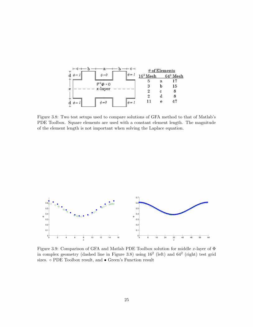
Figure 3.8: Two test setups used to compare solutions of GFA method to that of Matlab’sPDE Toolbox. Square elements are used with a constant element length. The magnitudeof the element length is not important when solving the Laplace equation.

0 2 4 6 8 10 12 14 160

0.1

0.2

0.3

0.4

0.5

0.6

z

Φ

0 8 16 24 32 40 48 56 640

0.1

0.2

0.3

0.4

0.5

0.6

0.7

z

Φ

Figure 3.9: Comparison of GFA and Matlab PDE Toolbox solution for middle x -layer of Φin complex geometry (dashed line in Figure 3.8) using 162 (left) and 642 (right) test gridsizes. ◦ PDE Toolbox result, and • Green’s Function result

25

3.3.3.1 Modifications to the Complex Green’s Functions and the Assembly

Technique

Finally, to lower memory costs for the slit nanopore geometry, a “compressed”

Green’s function array was established. The inner regions of the upper and lower electrodes

in the slit nanopore geometry were previously zero, and the zeros were needed to help

provide the rectangular structure that was necessary for utilizing the GFA method (the

zeros are not present in the parallel plate geometry). However, by providing a structure

within the GFA numerical code, the zeros are removed from the Gi. A calculated memory

savings of ≈ 28% was observed, without adversely affecting computational time. The new

GFA method, which uses compressed green’s functions, was tested and compared with

results based on the iterative method. Testing validated that the updated method had no

affect on the results. Confirmation of accurate assembly allowed for the in-house code to

be confidently added to the chosen MD package.

3.3.4 Additions to PME in Gromacs

The GFA algorithm is implemented within a correction force algorithm that is added

to the MD software package Gromacs. Algorithm 2 self-consistently solves for the correction

force on each molecule so that the potential on the electrode equals to the applied potential.

Algorithm 2 Comments:

1. The FFT mesh of the PME was made equal to that of the Green’s function mesh.

2. A fourth order central finite difference scheme is used to calculate the electric field,

Ec, for the internal nodes. For example, the x-component of Ec at a point i,j,k is

computed by

Exc i,j,k =

φi−2,j,k − 8φi−1,j,k + 8φi+1,j,k − φi+2,j,k

12∆x(3.14)

Forward difference is used for nodes near an electrode that is located at a node 0. The

26

Algorithm 2 Force Correction using GFA

1: Find the φc at each electrode mesh point i by summing the reciprocal potential, φk,and the real potential φreal.

φc,i = φk,i + φreal,i (3.10)

a. Obtain φk from the PME method. This is calculated by a fast Fourier transformwithin Gromacs1.

b. Calculate the φreal by

φreal,i =

Nj∑

j=1

qj

4π εsol rj,ierfc(γ rj,i) (3.11)

where qj is particle charge, γ is the Ewald coefficient, Nj is the total number ofparticles, and r j,i is distance from the particle j to the electrode mesh point i.

2: Use GFA algorithm to obtain the potential field, Φc, based on the electrode potentialsφc.

3: Use Φc to obtain the Electric Field on the nodes using Equations 3.14 through 3.16 2,

Ec = ∇Φc (3.12)

4: Use Ec to obtain the correction force Fc3 .

Fc = E qi (3.13)

5: Add Fc to PME force

27

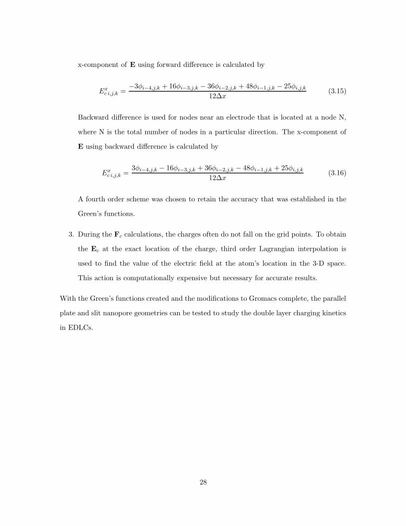
x-component of E using forward difference is calculated by

Exc i,j,k =

−3φi−4,j,k + 16φi−3,j,k − 36φi−2,j,k + 48φi−1,j,k − 25φi,j,k

12∆x(3.15)

Backward difference is used for nodes near an electrode that is located at a node N,

where N is the total number of nodes in a particular direction. The x-component of

E using backward difference is calculated by

Exc i,j,k =

3φi−4,j,k − 16φi−3,j,k + 36φi−2,j,k − 48φi−1,j,k + 25φi,j,k

12∆x(3.16)

A fourth order scheme was chosen to retain the accuracy that was established in the

Green’s functions.

3. During the Fc calculations, the charges often do not fall on the grid points. To obtain

the Ec at the exact location of the charge, third order Lagrangian interpolation is

used to find the value of the electric field at the atom’s location in the 3-D space.

This action is computationally expensive but necessary for accurate results.

With the Green’s functions created and the modifications to Gromacs complete, the parallel

plate and slit nanopore geometries can be tested to study the double layer charging kinetics

in EDLCs.

28

Chapter 4

Electric Double Layer Kinetics in a

Parallel Plate Geometry

In Chapter 3, we discussed the tools and methodology behind solving the charging

kinetics based on circuit models, continuum models, and MD simulation. In this chapter,

we will describe how those tools are implemented, and the results of the implementation

for the parallel plate geometry. Two systems with different electrolytes will be analyzed:

the first an aqueous, and the second an organic electrolyte. The accuracy of the PNP and

circuit models for each electrolytic system will be compared against MD simulation results.

Before undertaking this task, however, the MD charging kinetics for each electrolyte will

be discussed in depth.

4.1 Aqueous Electrolyte Charging Kinetics

For the parallel plate geometry, testing began with an aqueous solution of Na+

and Cl− ions . The solution is an 1:1 electrolyte, thus the Debye length (Equation 2.1)

characterizes the length of the EDL. The force fields of the Na+ and Cl− ions are modeled

on tabular data in the literature of Patra and Karttunen[22], while the water is modeled on

the SPC/E potential.

29

4.1.1 MD Simulation Details

Independent starting configurations were created by building a single simulation of

ions in a water solvent with a pair of model electrodes separated by 3.3nm. To produce

an initial ionic concentration of C0 = 2M , 24 Na+ and Cl− ions are added to 728 water

molecules. The electrodes are comprised of 200 molecules in a square lattice. This initial

simulation was run with no potential drop between electrodes, and the temperature of the

system was set to 500K to bolster greater ion movement. Molecular positions during this

simulation were then saved at intermittent time increments. These positions became the

independent starting configurations for the charging kinetics.

Before simulating the charging kinetics using the independent starting configura-

tions, we must first find an equilibrium state of the ions at a temperature of 300K with

both electrodes at φ = 0. The independent starting configurations are ran until equilibrium

with φapplied = 0V on the positive and negative electrode. This step is important because

there are electrostatic forces that still occur in EDLCs before potentials are applied to the

electrodes. At the beginning of this stage, Gromacs was disallowed from generating new

velocities.

After equilibrium had been reached, impulse potentials of 0.5V, 1V, 2V, and 6V

were added to the positive electrode at t = 0. Each case was allowed to run for at least 300

ps, with an “on-fly” output every 2 ps. To examine the time-dependent data of the charging

process in MD, an “on-fly” code was added to output the number densities of the Na+ and

Cl− ions , as well as the hydrogen and oxygen atoms that make up the solvent. The output

represents the time-averaged data over 2 ps. The number densities are a function only

of the distance between the electrodes, thus the system can be considered 1-D, and only

number densities between the electrodes at a certain y- and z -position need to be found.

The five ion densities are then averaged over the independent cases, and form the backbone

behind all further post-processing procedures, including finding concentrations, potentials,

and charge densities.

Statistical results of C0 = 2M with an impulse φapplied = 0.5V, 1V, and 2V are

30

based on 140 independent starting configurations. An additional 104 independent cases

were also run for φapplied = 2V and C0 = 2M to confirm the accurately ran simulations.

For C0 = 2M with φapplied = 6V , 116 independent initial configurations were simulated.

Lower concentrations of Na+ and Cl− at C0 = 1M with φapplied = 1V were also simulated

using 140 independent configurations. To lower the ionic concentration, ions are removed

from the simulation box. A brief study of charging kinetics at C0 = 0.5M and φapplied = 2V

was performed using only 20 independent cases.

MD was also used to test a charging process where the potential is introduced as

quarter sine-wave instead of an impulse of potential. The quarter sine-wave test case is

performed to understand if water molecules are being affected adversely by the sudden

impulse of larger voltages. In this test, the potential is introduced more gradually to the

upper electrode by

φ = φ sin(πt

100ps), when t < 50ps

φ = φ, when t ≥ 50ps.

With this function, the φ is applied gradually, but is still continuous at 50 ps. The results of

the quarter sine-wave simulations are based on 84 independent configurations at C0 = 2M

and φapplied = 0.5V, 1V, and 2V.

A mesh of 30×25×25 square elements of length δL = 0.11 nm was used to discretize

the domain for PME and Green’s functions.

4.1.2 MD Simulation Results

4.1.2.1 Concentration Profiles

Calculation of the ion concentration profiles allows for understanding into the charg-

ing of the EDL. Figure 4.2 demonstrates the ionic concentration profiles as the system

advances toward equilibrium.

As the first peak of the Na+ grows, the difference between the Na+ and Cl−

concentration at that location also grows, and the speed at which this difference increases

31

0 1 2 30

2

4

6

8

time = 5 ps

Distance [nm]

Conc

entra

tions

[M]

0 1 2 30

2

4

6

8

time = 35 ps

Distance [nm]

Conc

entra

tions

[M]

0 1 2 30

2

4

6

8

time = 65 ps

Distance [nm]

Conc

entra

tions

[M]

0 1 2 30

2

4

6

8

time = 95 ps

Distance [nm]

Conc

entra

tions

[M]

0 1 2 30

2

4

6

8

time = 125 ps

Distance [nm]

Conc

entra

tions

[M]

0 1 2 30

2

4

6

8

time = 155 ps

Distance [nm]

Conc

entra

tions

[M]

Figure 4.1: Concentration evolution for C0 = 2M with φ = 0 at x = 0 and φ = φapplied = 2Vat x = 3.3nm. Na+ (solid) and Cl− (dashed).

32

relays information about the rate of the charging kinetics. The middle of the concentration

profile will stay at the initial concentration, C0, until the system nears equilibrium. This

area is considered the “bulk”, and is represented by a resistor in the circuit model of charging

kinetics.

By comparing Figure 4.2 against Figure 4.1, one can see that different applied

potentials will affect the concentration profiles in two primary ways. First, decreasing the

potential drop between electrodes will decrease the height of the “first” counterion peak,

which is typically the location for both the highest counterion concentration and the largest

concentration difference between ionic species. In the case of Cl− ion concentration at a

∆φ = 1V , double peaks are shown to form at the electrode, with the Cl− peak closest to

the electrode forming more slowly. Secondly, by increasing the potential drop it is typical to

have lower Na+ concentrations near the positive electrode as a result of the increased force

on the ion by the larger electric field, and the same is true for Cl− ions near the positive

electrode.

Figure 4.3 shows that at a 6V potential difference the “first” peak of the Na+ near

the negative electrode has been shifted closer to the electrode by approximately half the

distance, and the ions have become significantly more concentrated at the electrode. This

implies that ions are losing their solvation shells and moving closer to the electrode due the

increased electrostatic forces at the larger voltages. Also at a 6V potential drop, the Na+

ion peak shows a significantly higher concentration peak than the Cl−, which is a result of

the difference in bare diameter (2 A for the Na+ and 3.6 A for the Cl−).

Changing the concentration, as opposed to the potential, does little to affect the

trend that occurs in the concentration profiles. The difference that occurs between ion

concentrations in Figure 4.4 at the “first” peaks are equivalent to those found in the C0 =

2M concentrations and little difference occurs as to the rates at which the ions reach such

concentrations.

33

0 1 2 30

1

2

3

4

5

time = 5 ps

Distance [nm]

Conc

entra

tions

[M]

0 1 2 30

1

2

3

4

5

time = 35 ps

Distance [nm]

Conc

entra

tions

[M]

0 1 2 30

1

2

3

4

5

time = 65 ps

Distance [nm]

Conc

entra

tions

[M]

0 1 2 30

1

2

3

4

5

time = 95 ps

Distance [nm]

Conc

entra

tions

[M]

0 1 2 30

1

2

3

4

5

time = 125 ps

Distance [nm]

Conc

entra

tions

[M]

0 1 2 30

1

2

3

4

5

time = 155 ps

Distance [nm]

Conc

entra

tions

[M]

Figure 4.2: Concentration evolution for C0 = 2M with φ = 0 at x = 0 and φ = φapplied = 1Vat x = 3.3nm. Na+ (solid) and Cl− (dashed).

34

0 0.5 1 1.5 2 2.5 30

10

20

30

40

50

60

Distance [nm]

Conc

entra

tions

[M]

NaCl

0

50 time = 5 ps

0

50 time = 155 ps

Conc

entra

tion

[M]

0 0.5 1 1.5 2 2.5 30

50 time = 355 ps

time = equilibrium

Figure 4.3: Concentration evolution and equilibrium for C0 = 2M with φ = 0 at x = 0 andφ = φapplied = 6V at x = 3.3nm.

4.1.2.2 Potential Profile

The potential profile is another useful tool for understanding the charging process

of EDL capacitors. It provides useful insights into the potential and potential gradient in

the bulk, and the potential drop that occurs due to compact layer screening. Potential is

calculated by first finding the space charge density (ρe) using all five of the ions

ρe = −qO ∗ nd,O + qH ∗ nd,H1+ qH ∗ nd,H2

+ nd,Na − nd,Cl (4.1)

where qO and qH represent the charge of an oxygen and hydrogen atom respectively, and

nd,i representing the number density of each atom. After attaining the space charge density,

the potential is then solved by

− εsol∇2Φ = ρe (4.2)

35

0 1 2 30

1

2

3time = 5 ps

Distance [nm]

Conc

entra

tions

[M]

0 1 2 30

1

2

3time = 35 ps

Distance [nm]

Conc

entra

tions

[M]

0 1 2 30

1

2

3time = 65 ps

Distance [nm]

Conc

entra

tions

[M]

0 1 2 30

1

2

3time = 95 ps

Distance [nm]

Conc

entra

tions

[M]

0 1 2 30

1

2

3time = 125 ps

Distance [nm]

Conc

entra

tions

[M]

0 1 2 30

1

2

3time = 155 ps

Distance [nm]

Conc

entra

tions

[M]

Figure 4.4: Concentration evolution for C0 = 1M with φ = 0 at x = 0 and φ = φapplied = 1Vat x = 3.3nm. Na+ (solid) and Cl− (dashed).

36

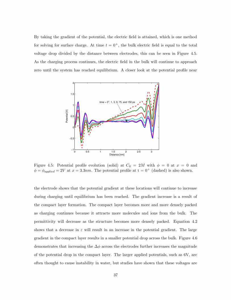
By taking the gradient of the potential, the electric field is attained, which is one method

for solving for surface charge. At time t = 0+, the bulk electric field is equal to the total

voltage drop divided by the distance between electrodes, this can be seen in Figure 4.5.

As the charging process continues, the electric field in the bulk will continue to approach

zero until the system has reached equilibrium. A closer look at the potential profile near

0 0.5 1 1.5 2 2.5 3−1

−0.5

0

0.5

1

1.5

2

Distance [nm]

Pote

ntia

l [V]

time = 0+, 1, 3, 9, 75, and 150 ps

Figure 4.5: Potential profile evolution (solid) at C0 = 2M with φ = 0 at x = 0 andφ = φapplied = 2V at x = 3.3nm. The potential profile at t = 0+ (dashed) is also shown.

the electrode shows that the potential gradient at these locations will continue to increase

during charging until equilibrium has been reached. The gradient increase is a result of

the compact layer formation. The compact layer becomes more and more densely packed

as charging continues because it attracts more molecules and ions from the bulk. The

permittivity will decrease as the structure becomes more densely packed. Equation 4.2

shows that a decrease in ε will result in an increase in the potential gradient. The large

gradient in the compact layer results in a smaller potential drop across the bulk. Figure 4.6

demonstrates that increasing the ∆φ across the electrodes further increases the magnitude

of the potential drop in the compact layer. The larger applied potentials, such as 6V, are

often thought to cause instability in water, but studies have shown that these voltages are

37

0 0.5 1 1.5 2 2.5 3−1

0

1

2

3

4

5

6

Distance [nm]

Pote

ntia

l [V]

time = 0+, 5, 20, 50, 100 ps

Figure 4.6: Potential profile evolution (solid) with C0 = 2M and with φ = 0 at x = 0 andφ = φapplied = 6V at x = 3.3nm, along with potential profile at t = 0+ (dashed).

“acceptable” when used in AC-EOF.

4.1.2.3 Surface Charge in the Channel Geometry

Charging kinetics can be quantified more easily by looking at the surface charge

density found on the electrodes. The surface charge density is defined as the amount of

charge per unit area on the electrode, and can be calculated in two ways: by integration of

charge density or by using the gradient of the potential. For both techniques, it is important

to understand how the space charge, ρe, is calculated. As mentioned in equation 4.1, the

space charge density can be calculated using every atom in the system, this has to be done

for the method that utilizes the gradient of the potential (∇Φ), because potential must be

calculated in this manner. The potential gradient (∇ΦofE) can be used to find the surface

charge density by

Q = εo ∗ ∇Φ (4.3)

38

This “gradient” method provides a better statistic, but does not start from zero surface

charge, as noted in Figure 4.7. On the other hand, surface charge density can also be

calculated by integrating ρe using

Q =

∫ w2

0ρe dx (4.4)

where is w is the width between electrodes. In this method, ρe can be calculated using all

the atoms (cf. Equation 4.1), or by using only the Na+ and Cl− ions so that the surface

charge is simplified as

Q = e

∫ w2

0(nd,Na+ − nd,Cl−) dx . (4.5)

Choosing to account for, or disregard the water atoms has very profound affects on the

numerical results of Q in the first 15 to 20 ps. Figure 4.7 demonstrates the affect. Without

0 50 100 1500

0.01

0.02

0.03

0.04

0.05

0.06

0.07

0.08

0.09

0.1

Time [ps]

Surfa

ce C

harg

e De

nsity

, Q [C

/m2 ]

Integration without H2O

Integration with H2O

Gradient Method

Figure 4.7: Surface charge density for ∆Φ = 2V across electrodes and C0 = 2M .

the water, the Q is more logarithmic and begins from zero charge. When accounting for

the water, the trend of Q from the integral method becomes similar to that of the gradi-

ent method, but with weaker statistics. For the proceeding analysis, the integral method

39

without the water components will be utilized because the information about only the ion

movement is the most beneficial.

As shown in Figure 4.8, increasing the potential difference between the electrodes

increases the surface charge density. This increase, however, is proportional to the voltage,

so that total capacitance of Equation 2.7 remains relatively equivalent at all voltages.

0 50 100 150 200 250 3000

0.05

0.1

0.15

0.2

0.25

Time [ps]

Surfa

ce C

harg

e De

nsity

, Q [

C/m2 ]

0.5 V1.0 V

2.0 V

6.0 V

Figure 4.8: Surface charge density for various values of ∆Φ across electrodes and C0 = 2M .

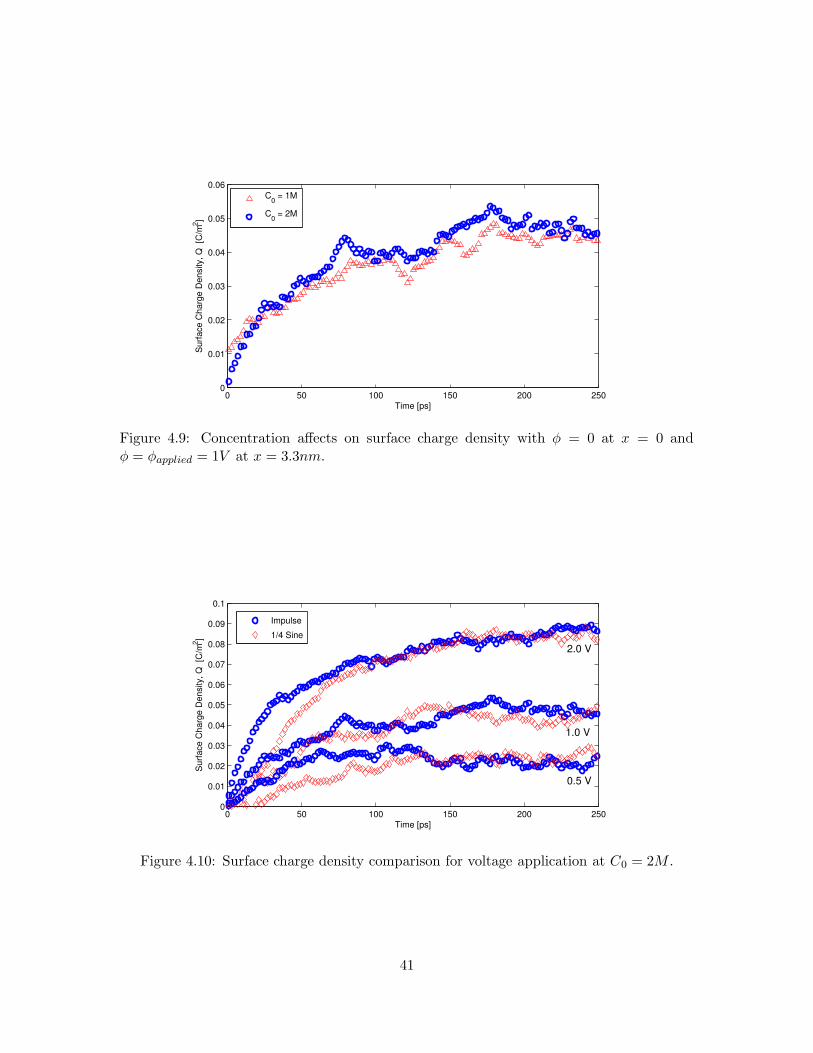
The effects of concentration change on Q are minimal. Figure 4.9 demonstrates

that although C0 is reduced by 50%, the trend of Q remains unchanged. As discussed in

Section 4.1.2.1, the concentrations for both species near an electrode have decreased equally,

therefore the concentration difference found in Equation 4.4 will remain the same for the

reduced concentration.

One interesting consideration is how the impulse applied potential affects the charg-

ing kinetics. A suddenly applied potential may cause adverse reactions in the solution. To

test the effect of the impulse, the Q of an impulse applied potential is compared in Figure

4.10 to a potential that was applied gradually using a quarter sine wave (cf Section 4.1.1).

As expected, charging is slowed in the first few tens of picoseconds due to the gradual po-

40

0 50 100 150 200 2500

0.01

0.02

0.03

0.04

0.05

0.06

Time [ps]

Surfa

ce C

harg

e De

nsity

, Q [

C/m2 ]

C0 = 1M

C0 = 2M

Figure 4.9: Concentration affects on surface charge density with φ = 0 at x = 0 andφ = φapplied = 1V at x = 3.3nm.

0 50 100 150 200 2500

0.01

0.02

0.03

0.04

0.05

0.06

0.07

0.08

0.09

0.1

Time [ps]

Surfa

ce C

harg

e De

nsity

, Q [

C/m2 ]

Impulse 1/4 Sine

2.0 V

0.5 V

1.0 V

Figure 4.10: Surface charge density comparison for voltage application at C0 = 2M .

41

tential increase of the sine function. However, the trend of Q is largely unaffected. By this,

we conclude that suddenly applying an impulse charge does not cause unforeseen adverse

reactions in the solution.

The rate at which Q reaches equilibrium (Q∞) is characterized by the time constant,

τ . The MD results show that the charging kinetics of the electrolyte solution of Na+ and

Cl− has two time constants, as shown for a ∆Φ = 2V in Figure 4.11. The first τ occurs

before 20 ps and the second for times between 20 ps and the time corresponding to a 90%

charge. This has been found to be true for all voltages tested in MD simulation, including

a 6V potential difference.

The lower time scale in the first 20 ps can be attributed to the slow rotational motion

of the water molecules, consequently they do not effectively screen the electrode during this

time. As a result, the permittivity of water would decrease until the water molecules have

had sufficient time to rotate, which occurs at around 20 ps.

Just as the capacitance changes little as a result potential changes, τ also changes

very little as a result of potential increases or decreases (cf. Figure 4.12); within the range

of voltages tested in this thesis. As a result of inconsequential effects of voltage and concen-

tration on Q and τ , analysis of the continuum and circuit models will be limited to potential

drops of 2V at C0 = 2M . These parameters were selected because they provide excellent

statistics in the MD results. The statistics of the MD results were found to be enhanced at

higher voltages compared to equal numbers of independent starting configurations at lower

voltages (cf. Figure 4.12).

4.1.3 Continuum and Circuit Models

For the continuum and circuit models of the aqueous electrolyte, the 1-D system

has a domain length of 2.58 nm, which corresponds to the approximate distance between

compact layers. The mobilities of Na+ and Cl− ions are 2.107 ×10−8 and 3.37 ×10−8 m2

V s,

respectively. A total of 128 uniform elements were used to discretize the domain in the

PNP model. The effective Stern layer thickness has a magnitude ranging from 5-10nm, and

42

0 50 100 150

−1.2

−1

−0.8

−0.6

−0.4

−0.2

0

Time [ps]

log(1

-Q/Q∞

)

1

MD Dataτ at time < 20 psτ at time > 20 ps

τ = 36.84 ps

τ = 71.3 ps

Figure 4.11: MD simulation charging kinetics for ∆Φ = 2V between electrodes and C0 =2M . The time scales are represented here as lines. At t < 20ps (dashed) τ = 36.84ps andt > 20ps (solid) τ = 71.3ps.

43

0 50 100 150−1.5

−1

−0.5

0

Time [ps]

log(

1−Q

/Q∞

)

φ = 0.5Vφ = 1Vφ = 2Vφ = 6V

Figure 4.12: MD simulation charging kinetics for C0 = 2M at various values of ∆Φ acrossthe electrodes.

varies depending on the magnitude of the potential drop. The relative permittivity of water

for the PNP model is 78.4.

4.1.3.1 Concentration Profiles

The PNP concentration profiles follow a similar behavior as those of the molecular

dynamics, as shown in figure 4.13. The positively charged Na+ ions move toward the

electrode where zero potential is applied, and the Cl− move toward the electrode where the

positive impulse potential is applied. As a result, locations of high ionic concentration occur

at the respective electrodes, anions at the anode and cations at the cathode. Simultaneously,

there is movement of the cations away from the anode, and anions away from the cathode.

The oscillation which occurs in the MD concentration profile near the electrode can only

be seen in the MD simulations because it models water discretely, while the PNP equations

model water as a continuum.

44

0 0.5 1 1.5 2 2.5 30

1

2

3

4

5

6

7

8

9

10

Distance [nm]

Conc

entra

tions

[M]

NaCl

Figure 4.13: MD versus PNP(bold) equilibrium concentration profiles for aqueous elec-trolyte at C0 = 2M with φ = 0 at x = 0 and φ = φapplied = 2V at x = 3.3nm.

Within the PNP model, the equilibrium concentration profiles of the Na+ and Cl−

should, in fact, be symmetric, as shown in Figure 4.13 . However, during the charging

process the concentration profiles were found to be asymmetric. The asymmetry occurs as

a result of using different ion mobilities for the ions. As the charging process progresses,

the ion with the higher mobility, Cl− for the aqueous electrolyte, will move more quickly

toward the anode, while the Na+ will move more slowly toward the cathode. Thus, the

concentration profiles will be different during charging, but will be equivalent after the ions

at the electrodes have reached their maximum concentration. This asymmetric behavior

during charging has more significance than just affecting the concentration profiles. Since

the variation in mobilities cause the ions to move at different speeds both away from,

and toward the electrodes, then the space charge density will be affected since it is directly

proportional to the difference in ionic concentrations. As a result, the surface charge density

will also be affected, causing non-linearity in the time constant for the charging kinetics.

Figure 4.14 demonstrates that the system has an inherent slight non-linearity, however

the non-linearity is dramatically increased when the mobilities are not equivalent. This

45

significant non-linearity, however, occurs primarily after charging has reached equilibrium.

0 100 200 300−0.5

0

0.5

1

1.5

2

2.5

3

3.5

4

Time [ps]

% N

on−L

inea

rity

of T

ime

Cons

tant

0 100 200 300−5

0

5

10

15

20

25

Time [ps]

Figure 4.14: Non-linearity if PNP charging with equivalent mobilities(right) and MD-basednon-equivalent mobilities(left). The plot is normalized as the percentage error from linearcharging based the minimum τ value, which occurs at approximately 130 ps.

4.1.3.2 Potential Profile

A look at the equilibrium potential profile of the continuum model in Figure 4.15

shows that most of the voltage drop occurs within the effective Stern layer, λS. In fact,

without accounting for λS , the continuum model is able to handle only lower potentials

(< 50mV ).

4.1.3.3 Surface Charge Density

If the Circuit or PNP model is going to be able to accurately predict charging

kinetics, they must have equivalent time constants, τ , to the MD simulations. Previously it

was proven by MD simulation that the τ of the channel geometry is linear (cf. Figure 4.11,

at least until 90% charged, which is considered most relevant to engineering applications).

The linearity supports the idea that the simple circuit model is qualitatively sufficient. A

46

0 0.5 1 1.5 2 2.5 30.95

0.96

0.97

0.98

0.99

1

1.01

1.02

1.03

1.04

1.05

Pote

ntia

l (V)

Position (nm)

52.8 mV

Figure 4.15: Potential profile from PNP model for φ = 0 at x = 0 and φ = φapplied = 2V atx = 3.3nm with C0 = 2M . Dashed lines represent the location of the electrodes in the inthe PNP model. With the boundary condition accounting for λs, the potential drop acrossthe bulk is reduced from 2V to only 52.8 mV.

further examination as to the quantitative accuracy of the circuit and PNP models show

that they provide a very capable model of predicting the τ at t > 20ps, as shown in Figure

4.16. The PNP and Circuit models have time τ = 72.5 ps and 74.27 ps respectively, which is

0 50 100 150

−1

−0.8

−0.6

−0.4

−0.2

0

Time [ps]

log

10(1

-Q/Q∞

)

1

MD DataMD curve fit t > 20 psPNP ModelCircuit Model

Figure 4.16: Charging Kinetics for an impulse applied potential of 2V at x = 3.3nm andφ = 0 at x = 0 with an initial ion concentration C0 = 2M .

only 1.6% and 4.1% larger than the MD prediction, and both fall within the ±5.2 statistical

error.

47

4.2 Organic Electrolyte Charging Kinetics

We next study the charging kinetics of EDLCs with an organic electrolyte which

consists of acetonitrile (ACN) with TEA+ and BF−

4 ions. The rod-like molecules of ACN

have shown the ability to withstand higher voltages than water without causing an elec-

trochemical reaction. TEA+ and BF−

4 are larger than their counterparts in the aqueous

electrolyte, but are still a 1:1 electrolyte due to their valence.

4.2.1 MD Simulation Details for the Organic Electrolyte

A single ionic concentration of 1.4M was simulated for the organic electrolyte by

placing 25 TEA+ and BF−

4 ions together with 260 molecules of ACN. The TEA+ ions

are modeled using the general AMBER force field (GAFF)[9], and the BF−

4 and ACN are

modeled based on force fields by Wang and coworkers[29]. The electrodes were formed

by a square lattice of 672 carbon atoms. The width between the electrodes is 3.74 nm.

Independent starting configurations were created in a similar fashion as described in the

aqueous system. The steps used in the aqueous electrolyte for creating the initial configu-

rations, finding the equilibrium state before applying a potential, and applying a potential

are equivalent in the organic electrolyte. An impulse 2.7V constant potential is applied to

one electrode (x = 3.74nm), and the other electrode (x = 0nm) is held at 0V.

4.2.2 Concentration Profiles

The concentration profiles of the organic electrolyte have similar trends as those

of the aqueous electrolyte, as shown in Figure 4.17 . Small concentration peaks near the

electrodes appear as the potential drop is applied, and these peaks continue to grow along

with a decline in the co-ion concentration until equilibrium has been reached. An interesting

phenomena that occurs in the organic electrolyte is the appearance of a small co-ion peak

that builds within a low concentration gap between the first two large concentration peaks.

This small peak continues to grow during the charging process, unlike the aqueous electrolyte

48

0 1 2 30

10

20

30

time = 5 ps

Distance [nm]Co

ncen

tratio

ns [M

]0 1 2 3

0

10

20

30

time = 300 ps

Distance [nm]

Conc

entra

tions

[M]

0 1 2 30

10

20

30

time = 900 ps

Distance [nm]

Conc

entra

tions

[M]

0 1 2 30

10

20

30

time = 1500 ps

Distance [nm]

Conc

entra

tions

[M]

Figure 4.17: TEA+ (solid) and BF− (dashed) concentration evolution for C0 = 1.4M withφ = 0 at x = 0 and φ = φapplied = 2.7V at x = 3.74 nm.

where the co-ions are only repelled from the electrode. By noting the times in the frames of

the concentration evolution, it can already be seen that the rate of charging in the organic

electrolyte will be much slower than that of its aqueous counterpart.

4.2.3 Potential Profiles

The evolution of the organic electrolyte potential profile in the channel mirrors that

found in the aqueous electrolyte. The potential gradient in the bulk continues to decline

from an initial state of ∇Φ = Φapplied/L at t = 0+, to ∇Φ = 0 at equilibrium.

4.2.4 Surface Charge Density

The time-dependent surface charge density of the organic electrolyte is shown in

Figure 4.19. As first noted in the concentration profiles in Figure 4.17, the charging rate of

the organic electrolyte demonstrated in Figure 4.20 is much slower than that of the aqueous

solution. However, this trend is expected because of the decreased mobility of the larger

ions in the ACN solvent. As with the aqueous electrolyte, two linear τ values characterize

49

0 0.5 1 1.5 2 2.5 3 3.50

0.5

1

1.5

2

2.5

Distance [nm]

Φ [V

]

time = 1, 10, 50, 250, 1000 ps

Figure 4.18: Potential profile evolution for organic electrolyte with C0 = 1.4M and φ = 0at x = 0 and φ = φapplied = 2.7V at x = 3.74 nm.

0 200 400 600 800 1000 1200 1400 1600 1800 20000

0.02

0.04

0.06

0.08

0.1

0.12

Time [ps]

Surfa

ce C

harg

e De

nsity

[C/m

2 ]

Figure 4.19: Surface charge density for C0 = 1.4M and ∇Φ = 2.7V .

50

the charging rate during 90% of surface charge accumulation. The decreased value of τ at

0 50 100 150 200 250 300 350 400 450 500

−1.2

−1

−0.8

−0.6

−0.4

−0.2

0

Time [ps]

log(

1−Q

/Q∞

)

MD Dataτ at time < 75 psτ at time > 75 ps

τ = 240.3 ps

τ = 107.5 ps

Figure 4.20: Characteristic charging rates and time constants for C0 = 1.4M and ∇Φ =2.7V .

t < 75ps in the organic electrolyte is thought to be caused by a similar effect as that found

in the aqueous electrolyte at t < 20ps.

4.2.5 Continuum and Circuit Models for the organic electrolyte

For the continuum and circuit model of the organic electrolyte, the 1-D system was

defined with a domain length of 3.15 nm, which is 0.59 nm smaller than the width between

electrodes used in the MD study. The smaller length accounts for the spaces between peak

and electrode, which are the compact layers (CL shown in Figure 4.21). The mobilities of

TEA+ and BF−

4 ions based on MD simulation are 5.5 ×10−9 and 8.8 ×10−9 m2

V s, respectively

[11]. The λs for C0 = 1.4M and ∆Φ = 2.7V is found to be 4.218 nm. The relative ACN

permittivity for the PNP model is 36. A total of 128 uniform elements were used to discretize

the domain in the PNP model.

51

4.2.5.1 Concentration profile comparisons

The concentration profiles of the TEA+ and BF−

4 in the PNP model follows similar

trends as those in its aqueous counterpart. Figure 4.21 shows that concentration peaks near

the electrodes are much lower than those of the MD. However, remember that the Q∞ of

the PNP model is made equivalent to the Q∞ of MD by by varying the the value of λs,

therefore both simulations must have an equivalent amount of ions near the electrode. Since

the ions in the PNP simulations are more spread out than those in the MD simulation, then

the peak of the ions in the PNP model must be lower in concentration.

0 0.5 1 1.5 2 2.5 3 3.50

5

10

15

20

25

30

Position (nm)

Conc

entra

tion

(M)

Concentration Comparison

TEABF4PNP TEAPNP BF4

CLCL

Figure 4.21: Concentration profile comparison between MD and PNP results for C0 = 1.4Mwith φ = 0 at x = 0 and φ = φapplied = 2.7V at x = 3.74 nm.

During post-processing of the continuum simulation results of the organic elec-

trolyte, it was found that the bulk concentration will begin to decline as the system nears

equilibrium. To validate the new PNP findings, the MD bulk concentration was calculated

by averaging the concentration in the middle 8 nodes. Figure 4.22 confirms that the bulk

concentration significantly declines at t > 1000 ps.

The decline in bulk concentration is a result of local ionic depletion, which is in-

troduced by Bazant et al. [4], and can be seen in Figure 4.23. At higher voltages, a large

amount of ions leave the “depletion area” (DA) and move closer to the electrode. As the

electrodes reach their maximum capacity, the ions that have moved near the electrodes

stay in the compact layer, and a concentration gradient (∆C/∆L as shown Figure 4.24)

52

0 500 1000 1500 2000 2500 3000 3500 40000.9

1

1.1

1.2

1.3

1.4

1.5

1.6

Time [ps]

TEA

Bulk

Conc

entra

tion

[M]

MDPNP Model

Figure 4.22: MD versus PNP(bold) bulk concentration decline for case of 2.7V potentialdrop with an initial organic electrolyte concentration of 1.4M.

occurs between the bulk and the “depletion area.” As a result, pure diffusion occurs from

the bulk to the “depletion area”, and the bulk concentration decreases. As expected, the

sharpest decline in bulk concentration occurs simultaneously with the largest gradient be-

tween the bulk and “depletion area”, as can be seen by comparing Figure 4.22 and Figure

4.24. Diffusion occurs throughout the charging process, but is maximized after charging

when the greatest concentration gradient occurs. Diffusion is much slower than electromi-

gration within the concentrations and voltages tested here, and as a result the linearity of

charging is not affected by diffusion until after Q reaches 90% of its equilibrium value.

0 0.5 1 1.5 2 2.5 31.2

1.22

1.24

1.26

1.28

1.3

1.32

1.34

1.36

1.38

1.4

TEA+ C

once

ntra

tion

[M]

Position [nm]

t = 20 ns

CDA Distance between CDA and CB

CB

t = 2 ns

(CB − CDA)

t = 400 ps

Figure 4.23: Time evolution of TEA+ concentration profile focusing on “depletion area”(DA) and bulk (B). Time steps are in increments of 100 ps.

53

The depletion and diffusion process was first noticed in the organic electrolyte be-

cause the diffusion coefficient of TEA+ and BF−

4 are much slower than those of their aqueous

counterparts. Due to its slower moving ions, the organic electrolyte has larger gradients and

slower diffusion rates, making the “depletion area” more visible upon inspection. However,

this process also occurs in the aqueous electrolyte simulations. When comparing equivalent

initial parameters, the gradients in aqueous simulations are often an order of magnitude

lower in scale, and the bulk to “depletion area” diffusion often is complete within a tenth

of the time it takes for the organic electrolyte to reach equilibrium in the bulk.

0 500 1000 1500 2000 2500 3000 35000

0.02

0.04

0.06

0.08

0.1

0.12

0.14

0.16

Time [ps]

Conc

entra

tion

Diffe

renc

e (C

B − C

DA) [

M]

0 500 1000 1500 2000 2500 3000 35000

0.5

1

1.5

2

2.5

Time [ps]

Dist

ance

bet

ween

CDA

and

CB

Figure 4.24: (Left) Time evolution of TEA+ concentration difference (∆C) between “de-pletion area” (CDA) and bulk (CB). (Right) distance between the x-locations (∆L) of CDA

and CB. Locations of CDA and CB are shown in Figure 4.23.

4.2.5.2 Voltage Profile Comparison

A comparison between the potential profile of the continuum model and that of

the MD simulation can be seen in Figure 4.25. First noted in the aqueous electrolyte, the

potential profile demonstrates that much of the potential drop in the PNP model occurs

within λS , and the potential drop across the bulk is minimal.

54

0 0.5 1 1.5 2 2.5 3 3.50

0.5

1

1.5

2

2.5

Pote

ntia

l (V)

Position (nm)

MDPNP

Figure 4.25: Organic electrolyte potential profile comparison of continuum model and MDsimulation for C0 = 1.4M with φ = 0 at x = 0 and φ = φapplied = 2.7V at x = 3.74 nm.

4.2.5.3 Surface charge density comparisons

The evaluation of the surface charge density by the PNP and RC model again

proved to be excellent. Figure 4.26 demonstrates that both models provide accurate results

for capturing τ between 75 and 500 ps. The models, however, can not accurately predict

τ before 75 ps because they do not model the solvent discretely, therefore capturing the

phenomena that causes the decreased value of τ (as discussed in Chapter 4) is not possible.

55

0 50 100 150 200 250 300 350 400 450 500

−1

−0.8

−0.6

−0.4

−0.2

0

Time [ps]

Log1

0(1−

Q/Q

∞)

MD DataRC (τ = 239 ps)PNP (τ = 236 ps)

Notes : Q∞ = 0.098217 (MD) is found by averaging Q from 2 to 3.6 ns

Figure 4.26: MD, circuit, and continuum model comparison for charging kinetics of theorganic electrolyte. The values for the RC and PNP model have been systemically loweredby 0.2 to ease comparison with the MD.

56

Chapter 5

Nanochannel Geometry Charging

Kinetics

To understand the affects of pore size on the charging kinetics, two pores widths of

0.66 nm and 0.77 nm were simulated using MD. The geometric dimensions are shown in

Figure 5.1. Square elements of length 0.11nm are used to discretize the domain for both

Figure 5.1: Schematic of geometric dimensions used for pore simulations.

the FFT and Green’s functions. As a result of the symmetric geometry, only 21 green’s

functions are needed to assemble the entire geometry for a 28 × 22 × 80 grid.

An aqueous electrolyte containing Na+ and Cl− ions was used in the system. The

same force field models that are used for the aqueous electrolyte in Chapter 4 are also used in

the slit nanopore geometries. The domain is filled with 1280 solvent molecules and 36 pairs

57

of the Na+ and Cl− ions. Independent initial positions are created just as for the parallel

electrode cases, by taking snap-shots of the positions at intermittent time intervals based

on a single simulation with a temperature at 500K. 90 independent starting configurations

were established for the nanopore geometries. The 90 independent configurations are then

simulated at 300K with a zero applied potential at both electrodes until they have reached

an equilibrium state. An impulse potential of 1V is subsequently applied to the anode, and

the cathode is held at 0V. The on-fly data of the nanopore simulations is different from

that of the parallel plate geometry. The nanopore on-fly code outputs the number of ions

that enter each pore just past the pore mouth. At this time, the ions outside the pore are

not studied.

5.1 Slit Nanopore Results

The surface charge density (Q) based on MD simulation of an aqueous electrolyte in

slit nanopores of width 0.66nm and 0.77nm are presented in this section. The equilibrium

Q is based on MD simulations performed by coworkers[11]. The surface density in each of

the electrode pore, Qanode,cathode, is determined by

Qanode,cathode =e (NNa − NCl)

area(5.1)

where NNa and NCl represent the number of ions in the pore. The magnitudes of Q on

the anode and cathode pores are then averaged to find Q for the entire system. The time

evolution of Q for pore widths of 0.66 nm and 0.77 nm are shown in Figures 5.2 and 5.3.

Since equilibrium results had already been attained, it was deemed unnecessary to run

simulations to complete equilibrium.

The charging kinetics of slit nanopores are found to be linear in nature (cf Equation

2.3) for both the 0.66 nm (Figure 5.4) and 0.77 nm (Figure 5.5) pore widths. As a result,

the charging characteristics of nanopores may be qualitatively captured by simple circuit

models.

58

0 500 1000 1500 2000 2500 3000 3500 4000 4500 50000

0.005

0.01

0.015

0.02

0.025

Time [ps]

Q [C

/m2 ]

Figure 5.2: Q for 0.66 nm slit nanopore during charging with φ = φapplied as shown inFigure 5.1. The solid line is non-equilibrium results, the dashed line is equilibrium results[11], and the dash-dot lines represent the error bar for the equilibrium calculation.

0 200 400 600 800 1000 1200 1400 16000

0.005

0.01

0.015

0.02

0.025

0.03

0.035

0.04

0.045

Time [ps]

Q [C

/m2 ]

Figure 5.3: Q for 0.77 nm slit nanopore during charging with φ = φapplied as shown in Figure5.1. The solid line is non-equilibrium results, the dashed line is equilibrium results[11], andthe dash-dot lines represent the error bar for the equilibrium calculation.

59

0 1000 2000 3000 4000 5000−1

−0.9

−0.8

−0.7

−0.6

−0.5

−0.4

−0.3

−0.2

−0.1

0

Time [ps]

log(

1−Q

/Q∞

)

MD DataMD Fit (τ = 2360ps)

Figure 5.4: Charging kinetics for 0.66 nm slit pore with φ = φapplied as shown in Figure 5.1.

Increasing the pore size makes it easier for solvated ions to enter the pore, thus

increasing both the capacitance and the rate at which equilibrium is reached. By increasing

the slit pore width by an additional 0.11 nm, the capacitance is approximately doubled

(cf. Figure 5.3), and τ is decreased by more than 75% (cf. Figure 5.5).

5.2 Modeling Systems with Multiple Nanopores using Con-

tinuum Methods

The pore sizes studied above are ill-suited for continuum modeling because the com-

pact layer length used to calculate λs in the boundary conditions is greater than the width

of the actual pores. On the other hand, the continuum model can provide interesting details

about pore-to-pore interactions in multi-pore systems, details that would be computation-

ally unreasonable to obtain in MD because of the size of the domain. The highly symmetric

geometry, along with the boundary conditions, used to model a nanoporous structure is

shown in Figure 5.6. Instead of using an implicit compact layer as described for the parallel

plate EDLC geometry in Equation 2.12, the multiple cylinders of the exohedral pore are

60

0 200 400 600 800 1000 1200 1400 1600

−1.2

−1

−0.8

−0.6

−0.4

−0.2

0

Time [ps]

log(

1−Q

/Q∞

)

MD DataMD Fit (τ = 530 ps)

Figure 5.5: Charging kinetics for 0.77 nm slit pore with φ = φapplied as shown in Figure 5.1.

modeled with an explicitly defined compact layer (gray area) of lower permittivity. The

transport equations are not defined in the the compact layer, and ions are restricted from

entering, just as would occur after the compact layer has formed. Outside the compact

layer, Nernst-Planck equations (Equation 2.8) without electroneutrality are used to model

ionic transport, and the domain is filled by an organic electrolyte with ionic mobilities of

5.5 and 8.8 ×10−9m2/(V · s) for the positive and negative species, respectively. Einstein’s

relation (Equation 2.9) is used to solve for the diffusion coefficients. The initial ionic con-

centration in the domain is uniform at C0 = 1.02M , and the concentration on the “outer”

boundaries are held at the constant C0, so as to represent an electrolytic reservoir.

The electrostatics in the system are defined by the Poisson equation, which can be

found in Equation 2.10 of Chapter 2. The organic solvent has a relative permittivity of

36, and the explicit compact layers (gray) are defined with a relative permittivity of 9.73.

Neumann boundary conditions are used to define all the non-cylinder boundaries for the

electrostatics. The potential on the outer edge boundary of the compact layer is continuous

with the bulk. The inner edge along the solid cylinder has an applied potential, φapplied,

61

Figure 5.6: Geometry and boundary conditions for studying the affects of multiple pores onsurface charge density using continuum models. Transport equation boundary conditionsare in normal font, bold font is used for the electrostatic boundary conditions, and italicized

font is used for geometrical information.

62

which is uniform over the entire circumference, as well as over all cylinders in the system.

The boundary conditions are shown on Figure 5.6.

The geometry has two important dimensions: the distance d between cylinders and

the radius of the cylinders Rp . The values of Rp and d are varied to obtain the effect of

each geometrical variable on the circumferential variation of surface charge density. The

centers of the two complete cylinders are at 45◦ from the x-axis. The compact layer has

thickness 0.943 nm. The “reservoir” boundaries are placed 3 nm from the nearest compact

layer boundary.

The compact layer capacitance is expected to follow simple electrostatic theory

which predicts

Ccompact =εcomp εo

Rp ln(Rp+Tc

Rp

), (5.2)

where εcomp is the relative compact layer permittivity, εo is the vacuum permittivity, and

Tc is the compact layer thickness. Figure 5.7 demonstrates the PNP results for compact

layer capacitance on a single cylinder, which identically follows Equation 5.2, and confirms

that capacitance will increase as cylinder size decreases.

1 2 3 4 5 60.095

0.1

0.105

0.11

0.115

0.12

0.125

0.13

Cylinder Radius [nm]

Capa

citan

ce [F

/m2 ]

PNP single poreES theory

Figure 5.7: Capacitance of a single cylinder resulting from electrostatic (ES) theory andPNP results.

Similarly to the continuum model of the parallel plate geometry, COMSOL was

used to solve the coupled Poisson and Nernst-Planck equations. The 2-D geometry was

63

created along with the boundary conditions as specified above. The domain is meshed with

triangular elements, and a more dense mesh is used near the cylinder and compact layer

boundaries. The solver is time dependent and uses the linear system solver UMFPACK.

5.2.1 Multipore Results

To understand the affects of cylinder interactions on the variation of surface charge

density, the above system is tested by varying both d and Rp , and comparing the results.

Figures 5.8 and 5.9 demonstrate the time evolution of surface charge density, Q, on cylinder

1 (cf. Figure 5.6) with different d and Rp values. Since the equilibrium surface charge

density, Q∞, will increase as a result of decreasing Rp , the non-dimensional value Q* is

used such that

Q∗ =Q

Qs∞

where Qs∞ is the equilibrium value of Q based on a single cylinder system.

0 50 100 150 200 250 300 3500

0.2

0.4

0.6

0.8

1

Degrees

Q*

t = 0+

t = 1 nst = 5 nst = 10 nst = 30 ns

Figure 5.8: Variation of surface charge density along circumference of cylinder 1 calculatedusing gradient method. The distance between cylinders d = 5 nm, the cylinder radiusRp = 5 nm, and φ = φapplied = 1V on all cylinder surfaces. Zero degrees correspondsto the bottom-most point of the cylinder circumference in the y-direction (cf. Figure 5.6).Clockwise rotation around the cylinder is considered positive.

64

The surface charge density, Q, around the cylinder circumference is initially zero

at t = 0, and begins to increase after the potential is applied at t = 0+. The cylinder

surfaces nearest to the concentration reservoir at 180◦ and 270◦ (cf. Figure 5.8) see the

most immediate increase in Q due to their relative ease of access to ions in the reservoir.

The dip between these two locations (at 225◦) is most likely due to the affects of interaction

with cylinder 2 (cf. Figure 5.6), as is the case with the lowest concentration occurring at

45◦. Dips in the surface charge do not appear to occur at the cylinder interaction locations

at 135◦ and 315◦ because these areas do not see symmetric entrance of the ions from the

reservoir, as occurs at the other two locations at 45◦ and 225◦. On the other hand, in

Figure 5.9 at t = 90 ns the impact from every cylinder interaction site can be seen to

cause variation in Q. At t = 90 ns, the ions have had sufficient time to reach all locations

uniformly. However, with increased time the cylinder interactions become a less significant

factor in affecting the magnitude of the variation of Q along the cylinder circumference. In

fact, in Figure 5.8 the surface charge around the circumference of the cylinder at t = 30 ns

varies by less than 0.2%. Increased simulation run time should result in a variation which

approaches zero.

The distance d does not have a significant effect on the final Q variation around the

cylinder. However, the distance between cylinders does affect the rate at which the cylinders

reach their final charged state. By noting the times referenced in Figures 5.8 and 5.9, one

can see that decreasing d will result in delayed charging on the inner cylinder surfaces, a

result of the slower rate at which ions can move through the decreased gap (0.114 nm when

d = 2nm compared to 3.114 nm when d = 5nm) between compact layers. Cylinder radius,

on the other hand, is believed to have little effect on the circumferential variation of Q,

but does have an effect on the magnitude of Q∞, as discussed in Equation 5.2 and Figure

5.7. Results of continuum analysis on the exohedral pore indicates that equilibrium energy

density will not be diminished by pore-to-pore interactions.

65

0 50 100 150 200 250 300 3500

0.2

0.4

0.6

0.8

1

Degrees

Q*

t = 0+

t = 1 nst = 5 nst = 10 nst = 50 nst = 90 ns

Figure 5.9: Variation of surface charge density along circumference of cylinder 1 calculatedusing gradient method. The distance between cylinders d = 2 nm, the cylinder radiusRp = 2 nm, and φ = φapplied = 1V on all cylinders. Zero degrees corresponds to thebottom-most point of the cylinder circumference in the y-direction (cf. Figure 5.6).

66

Chapter 6

Conclusions

Understanding the charging kinetics of the EDL is important for optimizing the

effectiveness of energy storage in EDLCs and steady fluid flow during AC-EOF. In this

thesis, we studied the charging kinetics of EDLs near planar electrodes and in slit nanopores.

The charging kinetics in nanoscale planar electrode EDLCs were studied using a circuit

model, PNP models, and MD simulation.

In the study of charging kinetics of EDLs near planar electrodes, it was discovered

the the charging kinetics are characterized by increased ion accumulation near the elec-

trode, and a decreasing electric field in the bulk. Areas of low ionic concentration, termed

“depletion areas”, were found to occur during charging in the PNP simulations. These

areas are located between the ionic concentration peaks near the electrode, and the ionic

concentration in the bulk. It was discovered that diffusion occurs into the “depletion areas”

from the bulk. However, because the ionic flux is very low during charging and is maximized

only as the charging process reaches equilibrium, it is concluded that diffusion would not

significantly affect the linearity of the charging process.

The results of parallel electrode MD simulation using aqueous and organic elec-

trolytes demonstrated a two step linear charging process that characterizes the first 90%

of charge accumulation, which is considered the most relevant to engineering applications.

The initial linear charging process, typically in terms of tens of picoseconds, is characterized

67

by an increased rate of charging due to lower solvent permittivity. The low permittivity

is believed to be a result of the solvent molecules not being fully rotated during the ini-

tial charging process. A second linear charging process follows the initial charging, and is

characterized by slower charging rates that continue until the process nears equilibrium.

Therefore, it can be concluded that circuit models, which predict linear charging processes,

are qualitatively capable of modeling charging kinetics in parallel electrode geometries.

The results of the PNP and circuit models demonstrate that both models are capable of

producing accurate values of the second time constant within the range of voltages and con-

centrations studied in this thesis. However during the initial charging regime, the continuum

and circuit models are incapable of accurately modeling the system.

Testing in slit nanopore geometries demonstrated that charging processes of slit

pores are also linear, leading to a conclusion that it is qualitatively possible to model a

slit nanopore using a circuit model, however an attempt to do so is not performed in this

thesis. The charging rates of the 0.66 nm pore was found to be slower than that of its 0.77

nm counterpart. This is contributed to increased difficulty of ion entrance into the pore, as

well as a possible decrease in the mobility of ions inside the pore.

Finally, a porous geometry modeled by an exohedral pore with multiple solid cylin-

ders was used to gain further understanding of the affects of interactions between nearby

charged cylinders. During the charging process, it was noted that variations in the surface

charge density around the solid cylinders occurred due to interactions between cylinders,

and that the distance between cylinders may affect the charging rate of certain surfaces

within the porous structure. However, results also indicated that although variations in the

surface charge density may exist because of interactions during charging, the variations at

equilibrium are relatively small, and it can be concluded that nearby charged cylinders do

not affect the overall capacity of a nanocylinder at equilibrium.

68

Bibliography

[1] V. S. Bagotsky. Fundamentals of Electrochemistry. John Wiley and Sons, New Jersey,second edition edition, 2006.

[2] A. J. Bard and L. R. Faulkner, editors. Electrochemical Methods: Fundamentals and

Applications. John Wiley and Sons, New York, second edition edition, 2001.

[3] P. Barrade. Energy storage and applications with supercapacitors. ANAE, 2003.

[4] M. Bazant, K. Thornton, and A. Ajdari. Diffuse-charge dynamics in electrochemicalsystems. Physical Review E, 70(2), 2004.

[5] J. O’M. Bockris, B. Conway, and E. Yeager. Comprehensive Treatise of Electrochem-

istry, volume 1. Plenum Press, New York, 1980.

[6] A. B. D. Brown, C. G. Smith, and A. R. Rennie. Pumping of water with ac electricfields applied to asymmetric pairs of microelectrodes. Physical Review E, 63(1):016305,Dec 2000.

[7] L. Cheng, P. Fenter, K. L. Nagy, M. L. Schlegel, and N. C. Sturchio. Molecular-scale density oscillations in water adjacent to a mica surface. Physical Review Letters,87(15):4, 2001.

[8] J. Chmiola, G. Yushin, Y. Gogotsi, C. Portet, P. Simon, and P. L. Taberna. Anoma-lous increase in carbon capacitance at pore sizes less than 1 nanometer. Science,313(5794):1760–1763, 2006.

[9] S. Crouzy, S. Berneche, and B. Roux. Extracellular blockade of k(+) channels by tea:results from molecular dynamics simulations of the kcsa channel. Journal of General

Physiology, 118(2):207–217, 2001.

[10] Department of Energy. Basic Research Needs for Electrical Energy Storage, April 2007.Report of the Basic Energy Sciences Workshop on Electrical Energy Storage.

[11] Guang Feng. personal communication, 2008–2009.

[12] D. Frenkel and B. Smit. Understanding Molecular Dynamics Simulations from algo-

rithms to applications. Academic Press, San Diego, second edition edition, 2002.

[13] S. Ghosal. Fluid mechanics of electroosmotic flow and its effect on band broadening incapillary electrophoresis. Electrophoresis, 25(2):214–228, 2004.

69

[14] N. G. Green, A. Ramos, A. Gonzalez, H. Morgan, and A. Castellanos. Fluid flow in-duced by nonuniform ac electric fields in electrolytes on microelectrodes. iii. observationof streamlines and numerical simulation. Physical Review E, 66(2), 2002.

[15] J.G. Hu, S. Goldman, C. G. Gray, and H. R. Guy. Calculation of the conductance andselectivity of an ion-selective potassium channel (irk1) from simulation of atomic scalemodels. Molecular Physics, 98(8):535–547, 2000.

[16] J. Huang, B. G. Sumpter, and V. Meunier. A universal model for nanoporous carbonsupercapacitors applicable to diverse pore regimes, carbon materials, and electrolytes.Chemistry - A European Journal, 14(22):6614–6626, 2008.

[17] M. Jayalakshmi and K. Balasubramanian. Simple capacitors to supercapacitors - anoverview. International Journal of Electrochemical Science, 3(11):1196–1217, 2008.

[18] R. Kotz, M. Hahn, and R. Gallay. Temperature behavior and impedance fundamentalsof supercapacitors. Journal of Power Sources, 154(2):550–555, 2006. Selected papersfrom the Ninth Ulm Electrochemical Days.

[19] C. Kuo, C. Wang, and C. Chang. Generation of directional eof by interactive oscillatoryzeta potential. Electrophoresis, 29(21):4386–4390, 2008.

[20] H. Lee, G. Kim, and C. Lee. Analysis for edlc application on electric railway system.Technical report, Korea Railroad Research Institute, 2007.

[21] Z. Li and K. Ito. The Immersed Interface Method. Society for Industrial and AppliedMathematics, 2006.

[22] M. Patra and M. Karttunen. Systematic comparison of force fields for microscopic sim-ulations of nacl in aqueous solutions: Diffusion, free energy of hydration and structuralproperties. Journal of Computational Chemistry, 25(5):678–689, 2004.

[23] A. Raghunathan and N. Aluru. Self-consistent molecular dynamics formulation forelectric-field-mediated electrolyte transport through nanochannels. Physical Review E,76(1), 2007.

[24] A. Ramos, A. Gonzalez, A. Castellanos, N. G. Green, and H. Morgan. Pumping ofliquids with ac voltages applied to asymmetric pairs of microelectrodes. Physical Review

E, 67(5):056302, May 2003.

[25] I. H. Shrivastava and M. S. P. Sansom. Simulations of ion permeation through apotassium channel: Molecular dynamics of kcsa in a phospholipid bilayer. Biophysical

Journal, 78(2):557–570, 2000.

[26] O. Teschke, G. Ceotto, and E. F. de Souza. Interfacial aqueous solutions dielectric con-stant measurements using atomic force microscopy. Chemical Physics Letters, 326(3-4):328–334, 2000.

[27] M. Tuckerman and G. Martyna. Understanding modern molecular dynamics: Tech-niques and applications. The Journal of Physical Chemistry B, 104(2):159–178, 2000.

70

[28] C. Vayenas, R. E. White, and M. E. Gamboa-Aldeco, editors. Modern Aspects of

Electrochemistry, volume 41. Springer Science, New York, 2007.

[29] X. Wu, Z. Liu, S. Huang, and W. Wang. Molecular dynamics simulations of room-temperature ionic liquid mixture of [bmim][bf4] and acetonitrilr by a refined force field.Physical chemistry chemical physics, 7(14):2771–2779, 2005.

[30] Z. Yuan, A. Garcia, G. Lopez, and D. Petsev. Electrokinetic transport and separationsin fluidic nanochannels. Electrophoresis, 28(4):595–610, 2007.

71